Accepted Manuscript

A robust weighted SVR-based software reliability growth model

Lev V. Utkin, Frank P.A. Coolen

PII: S0951-8320(18)30458-7DOI: 10.1016/j.ress.2018.04.007Reference: RESS 6126

To appear in: Reliability Engineering and System Safety

Received date: 26 February 2016Revised date: 10 January 2018Accepted date: 9 April 2018

Please cite this article as: Lev V. Utkin, Frank P.A. Coolen, A robust weighted SVR-based software reli-ability growth model, Reliability Engineering and System Safety (2018), doi: 10.1016/j.ress.2018.04.007

This is a PDF file of an unedited manuscript that has been accepted for publication. As a serviceto our customers we are providing this early version of the manuscript. The manuscript will undergocopyediting, typesetting, and review of the resulting proof before it is published in its final form. Pleasenote that during the production process errors may be discovered which could affect the content, andall legal disclaimers that apply to the journal pertain.

ACCEPTED MANUSCRIPT

Highlights

• New robust model for software reliability growth

• Novel support vector regression model

• New results to facilitate computation and implementation

• Excellent performance compared to standard model

• Many possible generalizations, variations and applications

1

ACCEPTED MANUSCRIPT

A robust weighted SVR-based software reliability growth model

Lev V. Utkin1, Frank P.A. Coolen2

1Telematics Department, Central Scientific Research Institute of Robotics and Technical Cybernetics,Peter the Great Saint-Petersburg Polytechnic University, St. Petersburg, Russia2Department of Mathematical Sciences, Durham University, United Kingdom

Abstract

This paper proposes a new software reliability growth model (SRGM), which can be re-garded as an extension of the non-parametric SRGMs using support vector regression topredict probability measures of time to software failure. The first novelty underlying theproposed model is the use of a set of weights instead of precise weights as done in theestablished non-parametric SRGMs, and to minimize the expected risk in the framework ofrobust decision making. The second novelty is the use of the intersection of two specific setsof weights, produced by the imprecise ε-contaminated model and by pairwise comparisons,respectively. The sets are chosen in accordance to intuitive conceptions concerning the soft-ware reliability behaviour during a debugging process. The proposed model is illustratedusing several real data sets and it is compared to the standard non-parametric SRGM.

Keywords: Imprecise contaminated model, pairwise comparisons, quadraticprogramming, software reliability growth model, support vector regression

1. INTRODUCTION

Software reliability is one of the most important factors in the software developmentprocess, which directly impacts on software quality. According to [1], software reliabilityis defined as the probability of failure-free software operation for a specified period oftime in a specified environment. One of the methods for analyzing software reliability is toconsider a software testing process, where defects of software are detected and removed. Asa result, the software reliability tends to grow. Therefore, in order to estimate the softwarereliability by using information from the software testing process, many software reliabilitygrowth models (SRGMs) have been developed and successfully verified and applied in manysoftware projects. As pointed out by several authors [2, 3, 4], most SRGMs can be dividedinto two large groups: parametric and non-parametric models.

Parametric SRGMs are generally based on assumptions about the behaviour of thesoftware faults and failure processes, usually in the form of some statistical characteristics,for example, probability distributions of time between failures of the software. Dependingon the initial data representation, parametric SRGMs can also be divided into the times-between-failures or time-dependent models and the nonhomogeneous Poisson process (NH-

Preprint submitted to Reliability Engineering and System Safety April 11, 2018

ACCEPTED MANUSCRIPT

PP) based models. The first type of models uses times between successive software failuresduring the testing or debugging period in order to predict some probability measures oftime to the next software failure. One of the best known software reliability models isthe Jelinski-Moranda model [5], which assumes that the elapsed time between failures isgoverned by the exponential probability distribution with a parameter (failure rate) that isproportional to the number of remaining faults in the software. The second type of modelsuses numbers of software failures observed in a given period of time in order to predicthow many software failures will be observed in a time period after the debugging process.The best known parametric models of the second type are the NHPP based SRGMs. Anexample of the NHPP models is the well known Goel–Okumoto NHPP model [6], whichassumes that the cumulative number of failures follows a Poisson process, such that theexpected number of failures in a given time interval after time t is proportional to theexpected number of undetected faults at time t. Since parametric SRGMs depend on apriori assumptions about the nature of software faults and the stochastic behaviour of thesoftware failure process, they have quite different predictive performances across variousprojects [2, 7].

Non-parametric SRGMs utilize machine learning techniques including artificial neuralnetworks, genetic programming and support vector machines (SVMs) to predict the soft-ware reliability. One of the important advantages of the models is that they usually do notuse any prior assumptions and are based only on fault history data. Many non-parametricSRGMs have been proposed in the literature [2, 3, 7, 8, 9, 10, 11, 12, 13, 14, 15, 16, 17, 18,19, 20, 21]. Contributions to this field are continuing, For example, Barghout [22] presenteda new non-parametric model which is based on the idea of separation of concern betweenthe long term trend in reliability growth and the local behaviour. Ramasamy and Lak-shmanan [23] proposed another non-parametric model applying an infinite testing effortfunction. Bal and Mohaparta [24] proposed a nonparametric method using radial basisfunction neural network for predicting software reliability. Some models using the machinelearning framework have been considered and reviewed by other authors [25, 26, 27]. Itshould be noted that most so-called non-parametric SRGMs are not non-parametric in thestrictest sense, because most models require some parameters to be assigned, for example,parameters of a kernel in SVMs. Nevertheless, we will use the term non-parametric forsuch models in order to distinguish them from models of the first type.

Among all learning techniques applied for constructing non-parametric SRGMs, weselect for consideration SVMs [28, 29]. Since many SRGMs can be regarded as special casesof regression models, we consider a learning technique known as support vector regression(SVR), which is a modification or a special case of the SVM. Many available non-parametricSRGMs are based on SVR [7, 11, 18, 30].

Numerical results with many non-parametric SRGMs based on the SVR confirm theadvantage of SVR [11]. However, although the SVR shows good learning performanceand is suitable for generalizations, there are some limitations of its practical use. A mainproblem in many projects is that there may only be few test data available. In this case,the use of SVR for constructing a SRGM may lead to incorrect results. Moreover, tuning

3

ACCEPTED MANUSCRIPT

parameters of learning algorithms are based on the procedure of cross-validation whichdivides the learning set into two subsets: training and testing. If there is only a smalltotal data set, then this division leads to even smaller training sets which cannot be usedto correctly construct the model. Incorrect results occurring in such a scenario as a resultof the SVR, where the expected risk as an error measure for minimization is replaced byan approximation, are called the ‘empirical expected risk’. This can be regarded as abound depending on the so-called VC dimension introduced by Vapnik [29]. The empiricalexpected risk causes problems for very small training data sets. A further problem of suchmodels is that all failures during a debugging process are viewed as equivalent. In otherwords, the first failures discovered in the test process have identical impact on the softwarereliability prediction as the last failures discovered in the debugging process. However,failures discovered in the early part of the debugging process may well be characterized by“simple” errors in software, which arise due to inattention or carelessness of a programmer.Once such errors have been removed, remaining failures, both those discovered later in thedebugging process and those that remain and hence may lead to failures after testing, aremore likely to share common features. Furthermore, there may be an effect of data ageingdue to possible substantial changes of software during debugging. We should also notethat an assumption about independence of times to failure in the model may be violated[31] because the experience of testers with the specific software is likely to grow during thedebugging process.

A possible way to overcoming the first problem mentioned above is by assuming a prob-ability distribution over the elements of the training set instead of the uniform distribution,and to use it in the optimization problem of minimizing the risk measure. However, thequestion arises how we can justify that a specific probability distribution is better than theuniform distribution which is used in the empirical risk measure. The second problem canbe overcome by assigning different weights to elements of the training set. In particular, asimple way is to assign ranked weights, with small weights assigned to the first elements ofthe training set (corresponding to the the early stages of the debugging process) and largerweights assigned to the later elements (corresponding to the later stages of the debuggingprocess). Of course, this leads to other natural questions about the validity of the assignedweights and how changes of weights may affect the reliability prediction.

Taking into account the above mentioned issues, we propose a new non-parametricSRGM based on the SVR. The main idea underlying the new SRGM is to replace preciseweights assigned to the elements of training data by a set of weights produced by means ofspecial rules. In other words, based on a small amount of training data, we construct a setof distributions. Then we can choose a single distribution from the set which maximizesthe expected risk in accordance with the minimax strategy as commonly used in theoriesand methods for decision support. The chosen distribution, as well as the bounds of theset of distributions, depend on the unknown reliability model parameters which have tobe computed. After substituting the “optimal” probability distribution into an expressionfor the expected risk, we can compute the optimal parameters of the regression modelby minimizing the risk measure over the set of values of parameters. The properties of

4

ACCEPTED MANUSCRIPT

normalized weights of elements are the same as those of probabilities, within the scope ofthe considered model. We will use the term ‘weights’ instead of ‘probabilities’.

Let us explain the selection of a single distribution from the set of distributions. Infact, by replacing the precise weights of training data with a set of weights, we equivalentlyreplace the expected risk measure with a set of risk measures such that every measurecorresponds to a weight distribution from the set of weights. If we take a convex andcompact set of weights, then it is easy to prove that the set of risk measures as a set ofexpectations makes up a closed interval with some lower and upper bounds. This impliesthat we have to choose a point inside the interval of risk measures in order to minimize thecorresponding risk measure and to get the SRGM parameters. That is why we apply theminimax or robust strategy as one of the strategies to deal with interval-valued functionals.According to the minimax strategy we select the upper bound of the interval for minimizingand for getting the model parameters. In other words, we maximize (the upper bound) theexpected risk over the set of distributions in order to minimize this upper bound over theSRGM parameters.

Another important novel idea underlying the proposed SRGM is that we consider theintersection of two sets of weights. The first set is produced by the linear-vacuous mixture orimprecise ε-contaminated model [32], which can be viewed as a generalization of the well-known ε-contaminated (robust) model [33, Section 4.2.]. The application of this modelrelaxes the uniform distribution of weights, but does not assign a precise distribution.The second set is produced by a set of linear comparative equalities which softly rank theweights. We again do not assign precise weights for ranking the elements of training data.The second set allows us to relax the strict ranking. Crucially, both these sets compensateeach other: the use of each set on its own would tend to lead to very imprecise predictionsof the software reliability after the debugging process, but the logical use of the intersectionof these sets leads to quite reasonable levels of imprecision.

Robust SVMs with sets of weights have been studied for classification problems [34, 35,36]. Similar ideas as in those models are applied to the SVR in this paper, which is thebasis for the proposed robust SRGM. The robustness stems from the statistical sense as atool for taking into account how the SRGM behaves under a perturbation of the underlyingstatistical model, i.e., under changes of the uniform distribution of weights in the empiricalrisk measure. The idea to use sets of weights in the form of imprecise statistical modelssuggests as name for the proposed SRGM in this paper: IWSRGM (Imprecise WeightSRGM).

The paper is organized as follows. The statement of the non-parametric SRGMs in theframework of the SVR is given in Section 2. A weighted extension of the SVR is consideredin the same section. The weighted SVR under the condition that weights of examples areonly known to belong to a compact and convex set is studied in Section 3. Propertiesand extreme points of two sets of weights and their intersection are provided in Section 4.Section 5 presents an algorithm for the new model and its application to various real datasets, to illustrate the proposed IWSRGM and to compare it to the standard non-parametricSRGM. Some conclusions and future scope of the research are provided in Section 6.

5

ACCEPTED MANUSCRIPT

2. WEIGHTED SVR AND THE NON-PARAMETRIC SRGM

We start by formulating the non-parametric SRGM in the general framework of predic-tive learning problems [28, 29, 37]. Parameters of the regression models are computed byminimizing a risk functional defined by a certain loss function and by a probability distri-bution of the noise. In regression analysis, we aim at estimating a functional dependencyf(x) between a set of sampled points X = (x1,x2, ...,xn) taken from Rm, and target valuesY = (y1, y2, ..., yn) with yi ∈ R. In the framework of machine learning, the regression prob-lem can be stated in the same way. We assume that there are n training data (examples)S = {(x1, y1), (x2, y2), ..., (xn, yn)}, in which xi ∈ Rm represents a feature vector involvingm features and yi ∈ R is an output variable. Let us write the function f(x) in the formf(x) = 〈a, φ(x)〉 + b, where a = (a1, ..., am), b are parameters of the function; φ(x) is afeature map Rm → G such that the data points are mapped into an alternative higher-dimensional feature space G; 〈·, ·〉 denotes the dot product. A learning machine has tochoose the function f(x) from a given set of functions, such that it optimally approximatesthe unknown dependency. This can be done in several ways, for example, by minimizingthe empirical expected loss, where the loss function represents a measure of difference be-tween the estimate f and the actual value y given by the unknown function at a point x.The standard SVR technique is to assume that the probability distribution of the trainingpoints is the empirical (non-parametric) probability distribution function whose use leadsto the empirical expected risk

Remp =1

n

n∑

i=1

l(yi, f(xi)).

Here l is the so-called ε-insensitive loss function with the parameter ε, which is definedas

l(y, f(x)) =

{0, |y − f(x)| ≤ ε,

|y − f(x)| − ε, otherwise.

Many realizations of the SVR use some distribution of weights w = (w1, ..., wn) insteadof the uniform distribution (1/n, ..., 1/n) over the sampled points S in order to incorporateprior knowledge about importance of the points. The expected risk in this case is of theform:

Rw =n∑

i=1

wil(yi, f(xi)). (1)

We assume here that the weights are non-negative and w1 + ...+ wn = 1.The parameters a and b are estimated by minimizing the following regularized risk

function:

RSVR,w =1

2〈a, a〉+ C

n∑

i=1

wil(yi, f(xi)).

6

ACCEPTED MANUSCRIPT

Here, the first term is the standard Tikhonov regularization or smoothness term [38]; C > 0is the constant “cost” parameter which determines the trade-off between the flatness of fand the amount up to which deviations larger than ε are tolerated [39].

Introducing slack variables ξi and ξ∗i , the problem of minimizing the regularized riskfunction can be written as follows:

minimize1

2〈a, a〉+ C

n∑

i=1

wi (ξi + ξ∗i ) (2)

subject to ξi ≥ 0, ξ∗i ≥ 0,yi − 〈a, φ(x)〉 − b ≤ ε+ ξi, (3)

〈a, φ(x)〉+ b− yi ≤ ε+ ξ∗i . (4)

The above problem can be written in its dual formulation utilizing Lagrange multipliersαi, α

∗i , i = 1, ..., n, as [40]

maximizen∑

i=1

yi(αi − α∗i )− εn∑

i=1

(αi − α∗i )

− 1

2

n∑

i,j=1

(αi − α∗i )(αj − α∗j )K(xi,xj), (5)

subject ton∑

i=1

(αi − α∗i ) = 0, (6)

0 ≤ αi ≤ Cwi, 0 ≤ α∗i ≤ Cwi, i = 1, ..., n. (7)

Here K(xi,xj) = 〈φ(xi), φ(xj)〉 is the kernel function, that is the inner product of the pointsφ(xi) and φ(xj) mapped into the feature space. We do not need to compute the functionφ(x) explicitly due to the kernels, as it can be seen from the optimization problem thatonly the kernels are used in the objective function. Typical examples of kernel functionsare linear, polynomial and Gaussian [41]. We will only use the Gaussian kernel, which isdefined as

K(x,y) = exp(−‖x− y‖2 /σ2

),

where σ is the kernel parameter determining the geometrical structure of the mappedsamples in the kernel space. The regression function f can now be written in terms of theLagrange multipliers as

f(x) =n∑

i=1

(αi − α∗i )K(x,xi) + b.

A simple expression for computing b can be found in [39].

7

ACCEPTED MANUSCRIPT

3. SVR WITH A SET OF WEIGHTS

Suppose that a weight vector, or distribution, belongs to a compact and convex set P ,i.e., it is produced by finitely many linear constraints. Let us consider how to deal withthis set of weights in the framework of the SVR.

First of all, we return to the expected risk (1). Since w ∈ P and the set P is convex,the corresponding set of RSVR,w is bounded by some lower and upper bounds for every setof values of a and b. The upper bound determines the well-known minimax (pessimistic)strategy. According to the minimax strategy, a vector w is selected from the set P such thatthe expected risk RSVR,w achieves its maximum RSVR,w for every fixed a and b. It shouldbe noted that the “optimal” vector w may be different for different values of parameters aand b. The minimax strategy can be explained in a simple way. We do not know a precisevector w and every vector from P can be selected. Therefore, we should take the “worst”distribution providing the largest value of the expected risk. The minimax criterion canbe interpreted as an insurance against the worst case because it aims at minimizing theexpected loss in the least favorable case [42]. This leads to the following optimizationproblem corresponding to the minimax strategy:

RSVR = mina,b

maxw∈P

(C

n∑

i=1

wil(yi, f(xi)) +1

2〈a, a〉

), (8)

subject to (3), (4) and w ∈ P .Let us fix the values a and b. Then we have a linear programming problem with variables

w and constraints P . The set P is compact and convex. Therefore, the optimal solutioncan be found among the extreme points of the set. If the number of extreme points is s,then the above problem is reduced to s standard optimization problems of the form:

R(k)SVR = min

a,b

(C

n∑

i=1

w(k)i l(yi, f(xi)) +

1

2〈a, a〉

), k = 1, ..., s, (9)

subject to (3), (4).

Here w(k)i is the i-th element of the k-th extreme point. After solving s programming

problems (9), we get s “local” solutions a(k) and b(k), k = 1, ..., s. The final optimal solutionof the problem corresponds to the largest objective function, i.e., we choose the parametersa(k) and b(k) with k = kopt such that

kopt = arg maxk=1,...,s

R(k)SVR.

It is interesting to note that extreme point w(kopt) is the “optimal” or “worst” distri-bution providing the largest value of the expected risk. When we deal with the dual form(5)-(7), the same procedure is carried out, but we take the variables αi, α

∗i , i = 1, ..., n,

instead of a and b.

8

ACCEPTED MANUSCRIPT

The above approach for solving the optimization problem is very simple when we knowthe extreme points. Therefore, the next problem is to determine the extreme points of asuitable set P which is relevant and interesting for SRGMs.

4. WEIGHTS FOR OBSERVATIONS AND THEIR EXTREME POINTS

The main idea proposed in this paper, in order to improve the SRGM, is to considertwo sets of weights. The first set is produced by the imprecise ε-contaminated model [32].Its use relaxes the uniform distribution of weights. The second set is produced by a set ofpairwise comparisons, which allows us to relax a strict ranking of weights in the sense thatwe do not assign precise weights for ranking the elements of the training data. The use of thefirst set of weights is a common way to robustify statistical models, particularly in case of asmall number of training data. The second set of weights reflects the different importanceof data obtained during the debugging process, where elements of the training set fromthe later stages of the debugging process are deemed to be more important than elementsfrom the earlier stages of this process. There are several reasons why this is attractive.First, particularly simple errors in the software are likely to be removed early on in thedebugging process. Secondly, there may be an effect of data ageing due to substantialchange of the software during debugging: by removing errors, a programmer may changesubstantial parts of the software. Hence, software failure data from the earlier stages ofthe debugging process may be less relevant for predicting the software’s future reliabilitythan data from the later stages, which can be reflected through the weights. Furthermore,the assumption about independence of times to failure may be violated. Cai et al. [31]pointed out that this assumption is not realistic in general, because test cases are usuallynot just selected at random but based on the previous experience with the software in thedebugging process.

Both sets of weights discussed above are important for constructing the SRGM, so weaim at benefitting from the advantages of both sets. Therefore, we use the intersectionof the sets to develop the new IWSRGM. This has the further important advantage that,while each of the two sets considered is rather large and would lead to overly pessimisticdecisions based on the minimax criterion, these two sets compensate each other and theirintersection reduces the size of P substantially, making the minimax criterion more suitablein order to reach robust but realistic inferences. From the perspective of computation, itis important to note that both these sets of weights are convex, and the intersection oftwo convex sets is also a convex set which is totally defined by its extreme points. Thisimplies that we can use the results obtained in the previous section in order to solve theprogramming problems (9) by determining the extreme points of the intersection of the twosets of weights. Next we present the two sets of weights in detail, followed by presentationof the intersection of these two sets.

9

ACCEPTED MANUSCRIPT

4.1. The linear-vacuous mixture set of weights

The linear-vacuous mixture or imprecise ε-contaminated models produce the set P(ε, w)of weights, or probabilities, w = (w1, ..., wn) such that wi = (1 − ε)pi + εhi, where p =(p1, ..., pn) is an elicited probability distribution, or the single probability distribution onewould expect to be most realistic, hi is arbitrary and h1 + ...+ hn = 1, 0 < ε < 1. The setP(ε, p) is a subset of the unit simplex S(1, n). Moreover, it coincides with the unit simplexwhen ε = 1. We denote the set P(ε, p) under condition p = (1/n, ..., 1/n) as P(ε). It canbe produced by n+ 1 hyperplanes

wi ≥ (1− ε)n−1, i = 1, ..., n, w1 + ...+ wn = 1. (10)

4.2. The set of weights produced by comparative information

Let us consider the following comparative information:

w1 ≤ w2 ≤ ... ≤ wn, (11)

and the condition w1 + ...+ wn = 1.A set M of weights w = (w1, ..., wn), which is produced by n − 1 inequalities of the

form wi − wi−1 ≥ 0, n inequalities wi ≥ 0 and one equality w1 + ...+ wn = 1, has extremepoints of the form:

w1 w2 ... w3 w4 wn

0 0 ... 0 0 10 0 ... 0 1/2 1/20 0 ... 1/3 1/3 1/3... ... ... ... ... ...

1/n 1/n ... 1/n 1/n 1/n

It is interesting to see that the extreme points correspond to cases for which only severalelements of the training data are used for constructing a regression model. Moreover, wehave two extreme cases. The first one is the distribution of weights having only one non-zero element. In this case, the decision is made on the basis of the last point. Anotherextreme case coincides with the uniform distribution, as used for the empirical expectedrisk.

4.3. Intersection of the two sets of weights

Before we study the intersection of general sets P(ε) and M, we consider this inter-section for the case n = 3 by using the standard unit simplex. Figure 1 illustrates theunit simplex, every point of which is a possible weight vector (w1, w2, w3). The set Mcorresponds to the area restricted by the triangle ABC. The set P(ε) corresponds to thearea restricted by the small simplex. Their intersection is restricted by the triangle BED(the shaded area). We can see from the figure that the obtained set of weights is quitesmall when compared to the two individual sets of weights. Furthermore, the weights inthe intersection, hence those used in the IWSRGM, are shifted towards the last (the third)

10

ACCEPTED MANUSCRIPT

Figure 1: Intersection of the two sets of weights in the unit simplex for n = 3

vertex of the simplex, which means that the final element of the test data tends to get mostweight. However, the simultaneous restriction to the small simplex corresponding to P(ε)prevents that the weight assigned to the last vertex becomes too large.

Now we turn our attention to the general case with n elements in the test data, forwhich the following proposition is crucial for computational feasibility of our proposed newmodel. The proof of this proposition is presented in the Appendix.

Proposition 1. The set of extreme points of the intersection P(ε) ∩ M consists of nelements of the form:

w1 = w2 = ... = wi−1 =1

n− ε

n,

wi = wi+1 = ... = wn =1

n+ε

n· i− 1

n− i+ 1,

i = 1, ..., n.

Proposition 1 provides the set of the extreme points of the set P(ε) ∩M, which arenecessary for solving the s = n programming problems (9). Every optimization problemis defined by one of the extreme points w(k), k = 1, ..., n. As a result, we have n standardweighted SVRs which can be easily solved.

Let us consider the set P(ε)∩M in more detail as it is very interesting, and we believeit is attractive for a robust SRGM. Condition (11) produces a rather large set of weightsM and its sole use could lead to quite unlogical results. In particular, one of the extremepoints ofM is (0, ..., 0, 1)., according to which the time to failure after the debugging processwould be predicted on the basis of only the last observation from that process. It is thereforeunlikely that one would want to use the entire set M to construct a robust SRGM. Theset of weights P(ε) also has shortcomings. In particular, if we look at its extreme points,

11

ACCEPTED MANUSCRIPT

then we observe that they consist of identical elements except for a single element whichis larger than the other elements. In particular if ε is quite large, the prediction of thetime to failure after the debugging process would be based substantially more on one of theelements of the test data than the other ones. The intersection of these sets P(ε) and M,however, avoids these problems and keeps attractive properties of both sets, in particularthe fact that the weights are somewhat larger towards the data from the later stages of thedebugging process but earlier data also keep some influence on the predictions. Finally,it is worth mentioning two special cases of the proposed IWSRGM. If ε = 0, then the setP(ε) ∩M is reduced to the single point (1/n, ..., 1/n), which corresponds to the standardSVR without considering sets of weights. The second extreme case occurs for ε = 1, whichleads to P(1) ∩M =M, which means that only the set of weights reflecting the pairwisecomparisons is used.

5. THE ALGORITHM FOR IWSRGM AND APPLICATIONS

In this section we present the algorithm for implementing the IWSRGM and we illustrateits application on six publicly available data sets. For each application, we randomly splitthe data set, consisting of n examples, into two subsets. One of these, the training set, isused to train (‘fit’) the model, while the subset of the remaining data, the test set consistingof ntest examples, is used to validate the model. For most data sets, we use about 20% ofexamples for testing, so ntest is about equal to 0.2n, the randomly selected examples fortesting are given the indices n−ntest+1, ..., n. Every regressor is computed by means of theweighted SVR with parameter ε = 0 of the so-called ε-insensitive loss function, for detailswe refer to [39]).

Since the main purpose of these examples is to show the application of the IWSRGMon simple problems which are easy to visualize, the hyperparameters are chosen withoutfine tuning. For all performed experiments, we quantify the prediction performance withthe normalized root mean square error measure (MSE), defined as

MSE =

√∑ntest

i=1 (yi − f(xi))2

ntest

.

Here yi and f(xi) are the actual value and the forecasted value for the time betweenthe (i − 1)-th and i-th detected software failure, respectively. This MSE is only used tocompare the application of different models to the same data set, hence it could also bedefined with the denominator outside of the square-root, it would make no difference forthese comparisons. The corresponding error measures for the standard and the IWSRGMalgorithms will be denoted MSEst and MSEImp. We will also use the relative absolutedifference between MSEs (RAMSE) which is defined as

RAMSE = |MSEst −MSEImp| /MSEst × 100.

All experiments use a standard Gaussian radial basis function (RBF) kernel, with kernelparameter σ (see Section 2). Different values for the kernel parameter σ and the “cost”

12

ACCEPTED MANUSCRIPT

parameter C have been tested and those leading to the best results have been used. Thisprocedure is realized by considering all possible values of σ and C in a predefined grid. Thegrid for σ is determined as 2v, where v = −15, ..., 0, ..., 15. The values of C are taken inaccordance with the expression C0 + iCs, where C0 and Cs are experimentally determinedparameters, i = 1, ..., 40.

Algorithm 1 describes the implementation of the IWSRGM in pseudo-code. The pro-posed IWSRGM has been evaluated and investigated using six publicly available data sets,taken from the literature, which all have different characteristics. The results are presentedand discussed in the following subsections.

Algorithm 1 The algorithm implementing the IWSRGM

Require: S (training set), parameters ε, ε, grid for σ ∈ {σ1, ..., σr}, grid for C ∈{C1, ..., Ct}

Ensure: f(xn+1){Straining, Stesting} : S ← Straining ∪ Stesting

i← 1; j ← 1repeatk ← 1repeatw ← w(k)

Solve problem (9) using w, σi, Cj and Straining

Compute R(k)SVR.

k + +until k > nkopt(i, j)← arg maxk=1,...,nR

(k)SVR

MSE(i, j)←MSE(kopt(i, j), Stesting, σi, Cj, wkopt(i,j))

i+ +; j + +until i > r; j > t(i, j)opt ← arg min(i,j)MSE(i, j)f(xn+1)←

∑ni=1(αi − α∗i )K(xn+1,xi) + b

5.1. Data Set 1

The first data set contains software inter-failure times taken from a telemetry networksystem by AT&T Bell Laboratories [43]. The data set contains 22 observations of theactual time series. The system receives and transmits data from a telemetry networkwhich consists of telemetry events such as alarms, facility-performance information anddiagnostic messages to operators for action. To test the system, system testers executedin a manner that emulated its expected use by system operators and other personnel. Thesystem was tested for three months until it was released to the beta site. After this, datawas collected for approximately another three months during beta-test execution [43, 44].

13

ACCEPTED MANUSCRIPT

Figure 2: Fault detection prediction results with two SRGMs for Data Set 1

Figure 2 presents the fault detection prediction results based on two SRGMs: thestandard non-parametric SRGM based on the SVR (the thin curve) and the IWSRGM(the thick curve), for which ε = 0.6 is used. The actual observations are also given (linkedby the dashed curve), where the training data are depicted by triangles and the testing databy circles. It seems that the actual data have substantial heteroscedasticity, i.e., changesof variance, in particular after the 15-th failure detection. In such a scenario, it seemsreasonable to base predictions more strongly on the observations from the later part of thetraining set than from the earlier part, as achieved by our method.

Figure 2 shows that the thin curve is close to most training points, especially at thebeginning of the debugging process. However, it behaves unsatisfactory for the testingperiod, where the large variation of times to failure is observed. At the same time, the thickcurve is more influenced by ‘anomalous’ points, which happens due to two reasons. First,the imprecise ε-contaminated model assigns larger weights to anomalous points becausethey increase the expected risk measure. Secondly, the set of weights produced by thecomparative information assigns smaller weights to points at the beginning of the debuggingprocess. The IWSRGM combines these two effects and performs better than the standardnon-parametric SRGM for the testing set.

To get more insight into the proposed IWSRGM, we investigate how the predictionperformance depends on the contamination parameter ε, by considering values at steps0.1 over the whole range 0 to 1 for ε. Note that ε = 0 corresponds to the standard non-parametric SRGM based on the SVR, as also used in Figure 2. Dependence of the MSE onthe parameter ε is shown in Figure 3. The solid curve corresponds to the MSE obtainedby using the proposed IWSRGM. The dashed line shows the MSE for ε = 0, i.e., for thestandard non-parametric SRGM. It should be noted that the solid curves and dashed linesin the similar figures for all later data sets, in the following subsections, will denote the

14

ACCEPTED MANUSCRIPT

Figure 3: Dependence of the MSE on the parameter ε, Data Set 1

MSEs for the IWSRGM and the standard SRGM, respectively. Figure 3 shows that theMSE of the IWSRGM is smaller than the MSE of the standard model for ε ≤ 0.6. Moreover,of the values considered, ε = 0.1 is optimal as it leads to the largest reduction of MSEs forthe IWSRGM compared to the standard SRGM.

5.2. Data Set 2

A further example of fault detection prediction results is shown in Figure 4, using datafrom a software inter-failure times series from [44], containing 101 observations. The twoSRGMs and the actual data are represented in the same manner as in Figure 2. Theobservations are characterized by large variation. As a consequence, the influence of theparameter ε on the MSE (see Figure 5) is quite weak: the largest RAMSE, at point ε = 0.7,is very small and equal to 1.7%.

5.3. Data Set 3

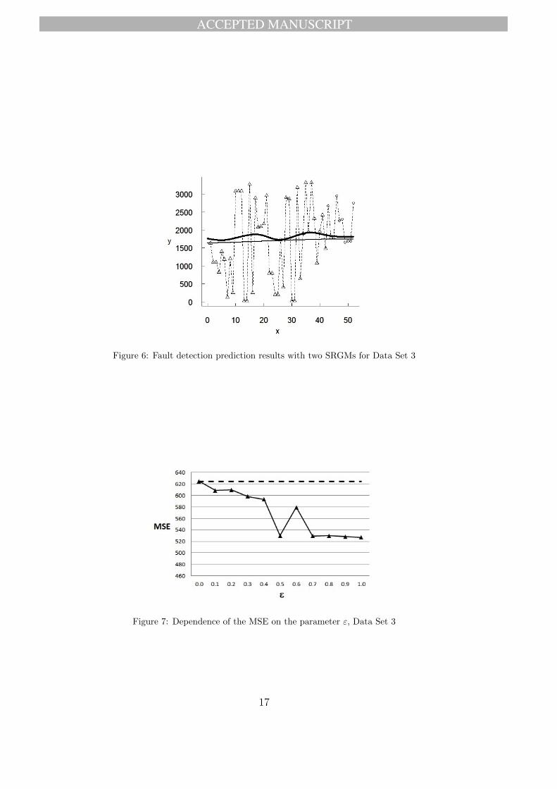
The next example uses data on helicopter main rotor blade part code, based on a systemdatabase collected from October 1995 to September 1999, as given in [45, Subsection 3.3.3].The data set consists of 52 observations. The results are shown in Figure 6. This showsthat variation of times to failure is rather large. Moreover, the reliability growth is almostinvisible. At first glance, the predicted results of the two models (standard SRGM andIWSRGM) are close, due to the large training set. However, we can see from Figure 7,which shows the dependence of the MSE on the parameter ε, that the largest RAMSE is15.6%, hence the IWSRGM provides a considerable improvement compared to the standardSRGM.

Figure 7 also shows that the MSE of IWSRGM is smaller than the MSE of the standardmodel for all ε. Some variation of the MSE as function of ε is caused by the small numberof testing data. It is important to point out that the set M of comparative informationitself (the case ε = 1) provides substantially better results than the standard model.

15

ACCEPTED MANUSCRIPT

Figure 4: Fault detection prediction results with two SRGMs for Data Set 2

Figure 5: Dependence of the MSE on the parameter ε, Data Set 2

16

ACCEPTED MANUSCRIPT

Figure 6: Fault detection prediction results with two SRGMs for Data Set 3

Figure 7: Dependence of the MSE on the parameter ε, Data Set 3

17

ACCEPTED MANUSCRIPT

Figure 8: Fault detection prediction results with two SRGMs for Data Set 4

Figure 9: Dependence of the MSE on the parameter ε, Data Set 4

5.4. Data Set 4

Next we show an example using data from testing an on-line data entry software packagedeveloped at IBM [46]. The data set contains 15 observations. The results are presentedin Figure 8. This is only a small data set, but there is clear reliability growth. Figure 9illustrates how the MSE depends on the parameter ε, it shows that the introduction ofthe set of weights together with the use of the minimax strategy, in our newly proposedmethod, leads to better results. The optimal value of ε = 0.4 as this corresponds to thelargest difference between the MSEs of the standard SRGM and the IWSRGM; the largestRAMSE is 6.3%.

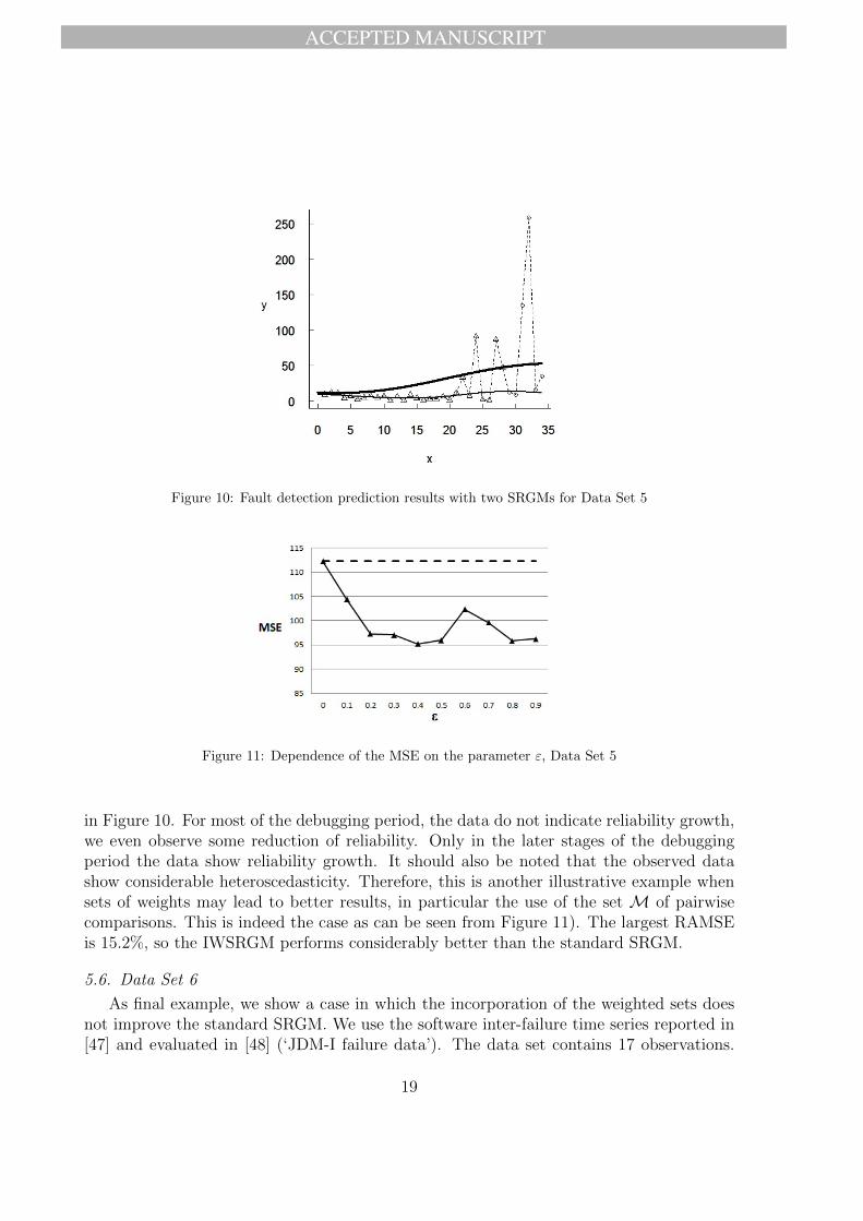
5.5. Data Set 5

Next we consider the NTDS failure data set, first reported in [5] and containing 34failure data. The data set can be also found in [45, Subsection 4.8]. The results are shown

18

ACCEPTED MANUSCRIPT

Figure 10: Fault detection prediction results with two SRGMs for Data Set 5

Figure 11: Dependence of the MSE on the parameter ε, Data Set 5

in Figure 10. For most of the debugging period, the data do not indicate reliability growth,we even observe some reduction of reliability. Only in the later stages of the debuggingperiod the data show reliability growth. It should also be noted that the observed datashow considerable heteroscedasticity. Therefore, this is another illustrative example whensets of weights may lead to better results, in particular the use of the set M of pairwisecomparisons. This is indeed the case as can be seen from Figure 11). The largest RAMSEis 15.2%, so the IWSRGM performs considerably better than the standard SRGM.

5.6. Data Set 6

As final example, we show a case in which the incorporation of the weighted sets doesnot improve the standard SRGM. We use the software inter-failure time series reported in[47] and evaluated in [48] (‘JDM-I failure data’). The data set contains 17 observations.

19

ACCEPTED MANUSCRIPT

Figure 12: Fault detection prediction results with two SRGMs for Data Set 6

Figure 13: Dependence of the MSE on the parameter ε, Data Set 6

The results are shown in Figure 12. The same examples were obtained for different valuesof ε. Here curves corresponding to the different SRGMs are very close to each other.Moreover, we can observe some reduction of the software reliability during the debuggingprocess. Figure 13 shows that the standard SRGM is better that the IWSRGM, but onlymarginally so as the largest RAMSE is 0.9%. Of course, ε = 0 reduces the IWSRGM tothe standard SRGM, so a search in the newly proposed model over the different values forε will indicate that the special case of the standard SRGM performs best for these data.

6. Concluding remarks

In this paper we have presented a new software reliability growth model (SRGM), calledImprecise Weight SRGM (IWSRGM), which can be viewed as an extension of the standardnon-parametric SRGMs using the SVR to predict probability measures of time to the next

20

ACCEPTED MANUSCRIPT

software failure. Two main ideas led to the proposed model. The first one is to use the setof weights instead of precise ones and to minimize the expected risk in the framework ofminimax (hence ‘pessimistic’) decision making. The second idea is to use the intersection oftwo specific sets of weights, which are chosen in accordance with some intuitive conceptionsconcerning the software reliability behaviour during a debugging process.

The IWSRGM is attractive from both the computation and development points of view,due to the representation of the complex optimization problem (8) by a finite set of standardquadratic programmes which implement the SVR. This representation requires knowledgeof the extreme points of the set of weights used for constructing the model, which waspresented in this paper. This also implies that variations to the proposed IWSRGM can bederived by using other sets of weights, as long as these sets are compact, convex and theirextreme points are known. This suggests an interesting topic for future research, namelyto construct different sets of weights corresponding to different software reliability growthscenarios.

Six examples with data sets from the literature have been presented. These have il-lustrated that the proposed IWSRGM tends to perform better than the standard non-parametric SRGM, although it is possible that no improvement may be achieved (DataSet 6). At the same time, we have observed that the quality of predictions depends onthe parameter ε of the linear-vacuous mixture or imprecise ε-contaminated model, whoseoptimal value is a priori unknown. It can be obtained only by considering all possible valuesin a predefined grid. These examples have shown that the proposed model may provideworse results in comparison with the standard non-parametric SRGM for some values ofε, especially for large values when the set of weights produced by pairwise comparisonsbecomes prevailing over the set produced by the imprecise ε-contaminated model.

This new model, like other software reliability growth models, can be used to provideinsight into the improvement of the software during a testing and debugging process. Itshould be noted that only the times-between-failures models for software reliability growthhave been studied in the paper. However, we do not foresee major difficulties in extendingthe proposed approach to the NHPP-based SRGMs, this is left as a topic for future research.Another direction for future research is incorporation of prior statistical knowledge into theSRGM, which may improve the predictive properties of the developed models.

Appendix: Proof of Proposition 1

Denote the set of inequalities (10) by P and the set of inequalities (11) by M . We donot include into P inequalities wi ≥ 0 because all points with wi = 0 for at least one i donot belong to the intersection P(ε)∩M. Let us consider the system of 2n− 1 inequalitiesfrom P and M . It is know that every extreme point satisfies n− 1 equalities from P ∩M .We study the following cases.

Case 1. All n− 1 equalities are from P . Then it is obvious that w1 = ... = wn = 1/n.

21

ACCEPTED MANUSCRIPT

Case 2. n − 2 equalities are from P , and 1 constraint is from M . This implies that thereis one strict inequality wi−1 < wi from P and one equality wk = n−1− εn−1 from M . Herewe have to consider two subcases. The first subcase is k ≥ i. Then

wi−1 < wi = wk = n−1 − εn−1.However, wi = wi+1 = ... = wn. Hence, w1 + ... + wn = 1 − ε < 1 and we have reached acontradiction. Therefore, this subcase does not give extreme points.

The second subcase is k < i. Then

w1 = w2 = ... = wi−1 =1

n− ε

n.

Then there holdswi + ...+ wn = 1−

(n−1 − εn−1

)i.

Hence, we get

wi =1− (n−1 − εn−1) i

n− i+ 1=

1

n+ε

n· i− 1

n− i+ 1.

This is an extreme point for a fixed i. Note that the extreme point obtained in Case 1 canbe regarded as a special case of Case 2 when i = 1.

Case 3. n− 3 equalities are from P , and 2 constraints are from M . This implies that thereare two strict inequalities wi−1 < wi and wj−1 < wj, i < j, from P , and two equalitieswk = n−1 − εn−1 and wl = n−1 − εn−1, k < l. The subcase with k ≥ i or l ≥ i is notconsidered here, it leads to a contradiction similar to first subcase in Case 2. Hence we canrestrict attention to the second subcase with k < i and l < i. Then we can write

w1 = w2 = ... = wi−1 =1

n− ε

n.

Suppose that ws = a, s = i, ..., j − 1, and ws = b, s = j, ..., n, i.e.,

wi = ... = wj−1 = a, wj = ... = wn = b.

Here due to inequalities wi−1 < wi and wj−1 < wj, we can write

1

n− ε

n< a < b.

The numbers a and b satisfy the following obvious condition:(

1

n− ε

n

)(i− 1) + a(j − i) + b(n− j + 1) = 1.

It can be seen that there are infinitely many values of a and b satisfying the above condition.This implies that we get an edge of the corresponding polytope. The same can be obtained,in similar manner, for the other cases where we take n − r equalities from P , and r − 1constraints from M . Consequently, Case 2 totally defines all extreme points, as was to beproved.

22

ACCEPTED MANUSCRIPT

Acknowledgements

The authors are grateful for useful comments by three reviewers which led to improvedpresentation and suggested further topics for future related research.

References

[1] Lyu, M.R. (1996). Handbook of Software Reliability Engineering. McGraw-Hill, NewYork.

[2] Li, H.F., Lu, M.Y., Zeng, M., Huang, B.Q. (2012) A non-parametric software reliabilitymodeling approach by using gene expression programming. Journal of InformationScience and Engineering, 28, 1145–1160.

[3] Hua, Q.P., Xie, M., Ng, S.H., Levitin, G. (2007). Robust recurrent neural networkmodeling for software fault detection and correction prediction. Reliability Engineeringand System Safety, 92, 332–340.

[4] Roy, P., Mahapatra, G.S., Rani, P., Pandey, S.K., Dey, K.N. (2014). Robust feedfor-ward and recurrent neural network based dynamic weighted combination models forsoftware reliability prediction. Applied Soft Computing, 22, 629–637.

[5] Jelinski, Z., Moranda, P.B. (1972). Software reliability research. In: W. Greiberger,editor, Statistical Computer Performance Evaluation, pp 464–484. Academic Press,New York.

[6] Goel, A.L., Okomoto, K. (1979). Time dependent error detection rate model forsoftware reliability and other performance measures. IEEE Transactions in Reliability,R-28, 206–211.

[7] Tian, L., Noore, A. (2005). Dynamic software reliability prediction: an approach basedon support vector machines. International Journal of Reliability, Quality and SafetyEngineering, 12, 309–321.

[8] Amina, A., Grunskeb, L., Colman, A. (2013). An approach to software reliabilityprediction based on time series modeling. The Journal of Systems and Software, 86,1923–1932.

[9] Cai, K.Y., Cai, L., Wang, W.D., Yu, Z.Y., Zhang, D. (2001). On the neural networkapproach in software reliability modeling. The Journal of Systems and Software, 58,47–62.

[10] Chiu, K.C., Huang, Y.S., Lee, T.Z. (2008). A study of software reliability growthfrom the perspective of learning effects. Reliability Engineering & System Safety, 93,1410–1421.

23

ACCEPTED MANUSCRIPT

[11] Jin, C., Jin, S.W. (2014). Software reliability prediction model based on supportvector regression with improved estimation of distribution algorithms. Applied SoftComputing, 15, 113–120.

[12] Kim, T., Lee, K., Baik, J. (2015). An effective approach to estimating the parametersof software reliability growth models using a real-valued genetic algorithm. Journal ofSystems and Software, 102, 134–144.

[13] Kumar, N., Banerjee, S. (2015). Measuring software reliability: A trend using machinelearning techniques. In: Q. Zhu and A.T. Azar, editors, Complex System Modellingand Control Through Intelligent Soft Computations, volume 319 of Studies in Fuzzinessand Soft Computing, pp 807–829. Springer, Berlin.

[14] Kumar, P., Singh, Y. (2012). An empirical study of software reliability prediction usingmachine learning techniques. International Journal of System Assurance Engineeringand Management, 3, 194–208.

[15] Li, H.F., Zeng, M., Lu, M.Y., Hu, X., Li, Z. (2012). Adaboosting-based dynamicweighted combination of software reliability growth models. Quality and ReliabilityEngineering International, 28, 67–84.

[16] Lou, J., Jiang, J., Shuai, C., Wu, Y. (2010). A study on software reliability predictionbased on transduction inference. In: Test Symposium (ATS), 2010, 19th IEEE Asian,pp 77–80, Shanghai.

[17] Lou, J., Jiang, J., Shen, Q., Shen, Z., Wang, Z., Wang, R. (2016). Software reliabilityprediction via relevance vector regression. Neurocomputing, 186, 66–73.

[18] Moura, M.d.C., Zio, E., Lins, I.D., Droguett, E. (2011). Failure and reliability predic-tion by support vector machines regression of time series data. Reliability Engineeringand System Safety, 96, 1527–1534.

[19] Pai, P.F., Hong, W.C. (2006). Software reliability forecasting by support vector ma-chines with simulated annealing algorithms. Journal of Systems and Software, 79,747–755.

[20] Xing, F., Guo, P., Lyu, M.R. (2005). A novel method for early software quality predic-tion based on support vector machine. In: Proceedings of the 16th IEEE InternationalSymposium on Software Reliability Engineering (ISSRE 2005), pp 1–10.

[21] Yang, B., Li, X., Xie, M., Tan, F. (2010). A generic data-driven software reliabilitymodel with model mining technique. Reliability Engineering and System Safety, 95,671–678.

24

ACCEPTED MANUSCRIPT

[22] Barghout, M. (2016). A two-stage non-parametric software reliability model.Communications in Statistics - Simulation and Computation. Early online version:doi:10.1080/03610918.2016.1189567.

[23] Ramasamy, S., Lakshmanan, I. (2017) Machine learning approach for software relia-bility growth modeling with infinite testing effort function. Mathematical Problems inEngineering, Article ID 8040346, 6 pages. doi:10.1155/2017/8040346.

[24] Bal, P.R., Mohapatra, D.P. (2017). Software reliability prediction based on radialbasis function neural network. In: Advances in Computational Intelligence, Sahana,S., Saha, S. (Eds). Advances in Intelligent Systems and Computing, vol 509. Springer,Singapore. pp.101-110.

[25] Algargoor, R.G., Saleem, N.N. (2013). Software reliability prediction using artificialtechniques. International Journal of Computer Science Issues, 10, 274–281.

[26] Begum, M., Dohi, T. (2017). A neuro-based software fault prediction with Box-Coxpower transformation. Journal of Software Engineering and Applications, 10, 288–309.

[27] Choudhary, A., Baghel, A.S., Sangwan, O.P. (2016). Software reliability predictionmodeling: A comparison of parametric and non-parametric modeling. In: Proceedingsof the 6th International Conference - Cloud System and Big Data Engineering, pp649–653.

[28] Hastie, T., Tibshirani, R., Friedman, J. (2001). The Elements of Statistical Learning:Data Mining, Inference and Prediction. Springer, New York.

[29] Vapnik, V. (1998). Statistical Learning Theory. Wiley, New York.

[30] Xing, F., Guo, P. (2005). Support vector regression for software reliability growthmodeling and prediction. In: Advances in Neural Networks – ISNN 2005, volume 3496of Lecture Notes in Computer Science, pp 925–930. Springer, Berlin.

[31] Cai, K.Y,, Wen, C.Y., Zhang, M.L. (1991). A critical review on software reliabilitymodeling. Reliability Engineering and System Safety, 32, 357–371.

[32] Walley, P. (1991). Statistical Reasoning with Imprecise Probabilities. Chapman andHall, London.

[33] Huber, P.J. (1981). Robust Statistics. Wiley, New York.

[34] Utkin, L.V., Zhuk, Y.A. (2014). Robust novelty detection in the framework of acontamination neighbourhood. International Journal of Intelligent Information andDatabase Systems, 7, 205–224.

25

ACCEPTED MANUSCRIPT

[35] Utkin, L.V., Zhuk, Y.A. (2014). Imprecise prior knowledge incorporating into one-classclassification. Knowledge and Information Systems, 41, 53–76.

[36] Utkin, L.V. (2014). A framework for imprecise robust one-class classification models.International Journal of Machine Learning and Cybernetics, 5, 379–393.

[37] Vapnik, V. (1995). The Nature of Statistical Learning Theory. Springer, New York.

[38] Tikhonov, A.N., Arsenin, V.Y. (1977). Solution of Ill-Posed Problems. W.H. Winston,Washington DC.

[39] Smola, A.J., Scholkopf, B. (2004). A tutorial on support vector regression. Statisticsand Computing, 14, 199–222.

[40] Tay, F.E.H., Cao, L.J. (2002). Modified support vector machines in financial timeseries forecasting. Neurocomputing, 48, 847–861.

[41] Scholkopf, B., Smola, A.J. (2002). Learning with Kernels: Support Vector Machines,Regularization, Optimization, and Beyond. MIT Press, Cambridge, Massachusetts.

[42] Robert, C.P. (1994). The Bayesian Choice. Springer, New York.

[43] Pham, L., Pham, H. (2000). Software reliability models with time-dependent hazardfunction based on Bayesian approach. IEEE Transactions on Systems, Man, andCybernetics, Part A, 30, 25–35.

[44] Pham, L., Pham, H. (2001). A Bayesian predictive software reliability model withpseudo-failures. IEEE Transactions on Systems, Man, and Cybernetics, Part A, 31,233–238.

[45] Pham, H. (2006). System Software Reliability. Springer, London.

[46] Ohba, M. (1984). Software reliability analysis models. IBM Journal of Research andDevelopment, 28, 428–443.

[47] Musa, J.D., Iannino, A., Okumoto, K. (1987). Software Reliability: Mesurement,Prediction, Application. McGraw-Hill, New York.

[48] Liu, J., Xu, M. (2011). Function based nonlinear least squares and application toJelinski–Moranda software reliability model. Preprint arXiv:1108.5185.

26