HAL Id: hal-02439982https://hal.inria.fr/hal-02439982v2

Submitted on 6 Apr 2020

HAL is a multi-disciplinary open accessarchive for the deposit and dissemination of sci-entific research documents, whether they are pub-lished or not. The documents may come fromteaching and research institutions in France orabroad, or from public or private research centers.

L’archive ouverte pluridisciplinaire HAL, estdestinée au dépôt et à la diffusion de documentsscientifiques de niveau recherche, publiés ou non,émanant des établissements d’enseignement et derecherche français ou étrangers, des laboratoirespublics ou privés.

A robust and efficient numerical finite element methodfor cables

Charlélie Bertrand, Vincent Acary, Claude-Henri Lamarque, Alireza TureSavadkoohi

To cite this version:Charlélie Bertrand, Vincent Acary, Claude-Henri Lamarque, Alireza Ture Savadkoohi. A robust andefficient numerical finite element method for cables. International Journal for Numerical Methods inEngineering, Wiley, 2020, 121 (18), pp.4157-4186. 10.1002/nme.6435. hal-02439982v2

A robust and efficient numerical finite element method for cables

Bertrand C.*, Acary V.†, Lamarque C.-H.*, Ture Savadkoohi A.*

March 2019

Abstract

Numerical simulation of cable systems remain delicate due to their geometrical non-linearity and also totheir intrinsic unilateral constitutive law. Indeed Finite Element approaches (if not implemented carefully) fail topredict accurate equilibrium for cable structures. The major issue to be addressed is the ill-conditioning, startingconfiguration and wrong choice of descent direction during iterative methods. An iterative scheme based on FiniteElement Method is presented to overcome this issue, even with large number of elements.

Keywords: Cable Structures Analysis, Finite Element Method, Unilateral Tension, Numerical Methods

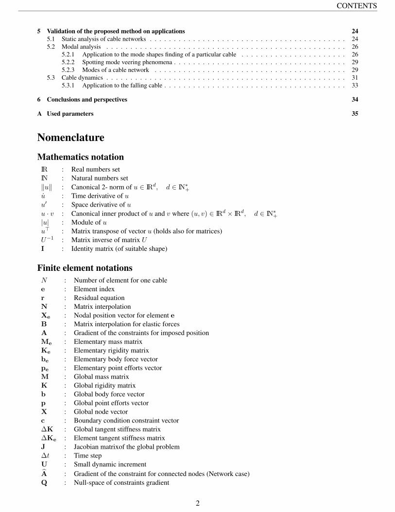
Contents1 Problem statement 4

1.1 Governing equations of the cable . . . . . . . . . . . . . . . . . . . . . . . . . . . . . . . . . . . . . . . . . 51.2 Closed form solution for the statics of the cable under self-weight loading . . . . . . . . . . . . . . . . . . . 6

2 Weak formulation of the non-dimensional problem 62.1 Non-dimensional form of the governing equations . . . . . . . . . . . . . . . . . . . . . . . . . . . . . . . . 72.2 Weak form of the equilibrium for a cable segment . . . . . . . . . . . . . . . . . . . . . . . . . . . . . . . . 7

3 Method 1: Standard FEM and spurious solutions 83.1 Finite element approximation . . . . . . . . . . . . . . . . . . . . . . . . . . . . . . . . . . . . . . . . . . . 83.2 Equality constraints for prescribed node positions . . . . . . . . . . . . . . . . . . . . . . . . . . . . . . . . 93.3 Non-admissible numerical solutions for the static analysis of the hanged cable . . . . . . . . . . . . . . . . . 103.4 Further discussion about the existence of non admissible cable equilibria . . . . . . . . . . . . . . . . . . . . 11

4 Method 2: A modified finite element formulation for cables 124.1 Axial forces reformulation and modified gradient . . . . . . . . . . . . . . . . . . . . . . . . . . . . . . . . 134.2 finite element approximation and modified Jacobian matrix . . . . . . . . . . . . . . . . . . . . . . . . . . . 154.3 Numerical hints: Methods 3 & 4 . . . . . . . . . . . . . . . . . . . . . . . . . . . . . . . . . . . . . . . . . 154.4 Numerical examples . . . . . . . . . . . . . . . . . . . . . . . . . . . . . . . . . . . . . . . . . . . . . . . 16

4.4.1 Effects of the rigidity . . . . . . . . . . . . . . . . . . . . . . . . . . . . . . . . . . . . . . . . . . . 184.4.2 Effects of point loads . . . . . . . . . . . . . . . . . . . . . . . . . . . . . . . . . . . . . . . . . . . 18

4.5 Heuristic convergence study . . . . . . . . . . . . . . . . . . . . . . . . . . . . . . . . . . . . . . . . . . . 214.5.1 Performance profiles . . . . . . . . . . . . . . . . . . . . . . . . . . . . . . . . . . . . . . . . . . . 214.5.2 Convergence with respect to mesh size . . . . . . . . . . . . . . . . . . . . . . . . . . . . . . . . . 234.5.3 Quadratic convergence of Modified Newton iterations . . . . . . . . . . . . . . . . . . . . . . . . . 234.5.4 Evolution of problem conditioning with regard to α . . . . . . . . . . . . . . . . . . . . . . . . . . . 24

*Univ Lyon, ENTPE, LTDS UMR CNRS 5513, Rue Maurice Audin 69518 Vaulx-en-Velin Cedex, France†Univ. Grenoble Alpes, CNRS, Inria, Grenoble INP (Institute of Engineering Univ. Grenoble Alpes) , GIPSA-Lab, 38000 Grenoble,

France

1

CONTENTS

5 Validation of the proposed method on applications 245.1 Static analysis of cable networks . . . . . . . . . . . . . . . . . . . . . . . . . . . . . . . . . . . . . . . . . 245.2 Modal analysis . . . . . . . . . . . . . . . . . . . . . . . . . . . . . . . . . . . . . . . . . . . . . . . . . . 26

5.2.1 Application to the mode shapes finding of a particular cable . . . . . . . . . . . . . . . . . . . . . . 265.2.2 Spotting mode veering phenomena . . . . . . . . . . . . . . . . . . . . . . . . . . . . . . . . . . . . 295.2.3 Modes of a cable network . . . . . . . . . . . . . . . . . . . . . . . . . . . . . . . . . . . . . . . . 29

5.3 Cable dynamics . . . . . . . . . . . . . . . . . . . . . . . . . . . . . . . . . . . . . . . . . . . . . . . . . . 315.3.1 Application to the falling cable . . . . . . . . . . . . . . . . . . . . . . . . . . . . . . . . . . . . . . 33

6 Conclusions and perspectives 34

A Used parameters 35

Nomenclature

Mathematics notationIR : Real numbers setIN : Natural numbers set‖u‖ : Canonical 2- norm of u ∈ IRd, d ∈ IN∗+u : Time derivative of uu′ : Space derivative of uu · v : Canonical inner product of u and v where (u, v) ∈ IRd × IRd, d ∈ IN∗+|u| : Module of uu> : Matrix transpose of vector u (holds also for matrices)U−1 : Matrix inverse of matrix UI : Identity matrix (of suitable shape)

Finite element notationsN : Number of element for one cablee : Element indexr : Residual equationN : Matrix interpolationXe : Nodal position vector for element eB : Matrix interpolation for elastic forcesA : Gradient of the constraints for imposed positionMe : Elementary mass matrixKe : Elementary rigidity matrixbe : Elementary body force vectorpe : Elementary point efforts vectorM : Global mass matrixK : Global rigidity matrixb : Global body force vectorp : Global point efforts vectorX : Global node vectorc : Boundary condition constraint vector∆K : Global tangent stiffness matrix∆Ke : Element tangent stiffness matrixJ : Jacobian matrixof the global problem∆t : Time stepU : Small dynamic incrementA : Gradient of the constraint for connected nodes (Network case)Q : Null-space of constraints gradient

2

CONTENTS

Physical quantityR : Axial forces in the cable (Vector valued function)e : Axial direction of the cable (Corresponding to the out-going normal of each sub-domains)ε : Axial strain of the cableL : Lagrangian length of the cable (Reference length or length at rest)EA : Rigidity of the cableb : Distributed body forces applied to the cable (Vector valued function)ρ : Linear density of the cablex : Position of the cable particles (Vector valued function)S : Lagrangian curvilinear abscissa (Reference curvilinear abscissa)g : Gravitational accelerationH,V,B : Initial horizontal, vertical and transverse components of the axial forcesω : Arbitrary frequency of the system

Introduction

Over the last two decades, cable structures have been investigated intensively due to their large spectrum of practical

engineering applications, which span from electric wires to aerial ropeways without forgetting cable stayed bridges

or cable networks. Theoretically, there is no uniform and standard framework to deal with the static or dynamic

equilibria of cables yet. Intensive research works are still going on in this domain due to their extremely nonlinear

behavior, although the catenary equation is known and solved since three centuries [1]. The diversity of cable

applications leads to a lot of coexisting frameworks until statics and dynamics (see the work of Irvine [2]).

Equilibria and dynamics of cable systems continue to be studied until today as it is reported in the detailed

review of Rega [3] with a focus on the modal analysis and the dynamics of cable systems. The temporal evolution

of these systems is treated with different approaches in the literature, for instance via the time integration of a

linearized system [4] or via studying reduced-order models before comparing them to results traced by a full Finite

Element Method (FEM) as done by Gatulli et al. [5] which topic was revisited later with a comparison to the

projected dynamics time integration by Warminski et al. [6]. Other theoretical developments have also been carried

out for studying statics of cable systems when more sophisticated equilibria are considered, for example, with an

intermediary pulley [7], for the dynamics of transmission lines by Tsui [8, 9] and also for galloping phenomena

studies via FEM by Desai et al. [10] or even for a cable network [11]. Various formulations exist for the cable

equations: one can formulate the equilibrium taking the displacements of nodes joined via the catenary solution

as unknowns [12], or formulating the equations using the current curvilinear abscissa [2], using a Lagrangian

configuration [13], directly in a discrete form [14] or via general principles of continuum mechanics [15]. Here

is chosen to work in the framework of curvilinear domains formulated with regards to a Lagrangian curvilinear

abscissa following [16].

Numerical methods for computing the behavior of cable structures are still an oncgoing research area. Starting

from the truss formulation of Ernst in 1965 [17], many attempts on FEM for cables have been done. Both in

statics, modal analysis (e.g.[18]) and in dynamics (e.g.[13]) some improvements and discussions raised and it still

continues. In most cases, cable problems are badly conditioned and the convergence results of the FEM techniques

are compromised [19]. Some improvements of the numerical procedure have been proposed to overcome this

issue by using numerical damping, load control step and a smart initial guess [20] or also constrained optimization

[14]. However, the problem remains stiff, badly scaled and ill-conditioned. Spurious solutions continue to be

3

observed [20], or the assumptions on the positive axial tension are not satisfied out of Gauss integration points [13].

Geometrically nonlinear aspects of the problem have been tackled using the absolute nodal constraint formulation

[21] where cable elements are successfully mixed with bar element and accounts for the axial force discontinuity

and also using co-rotational formulation [22]. In a recent work, Crussels-Girona et al. [15] design a proper mixed

finite element formulation for a neo-Hookean cable material with the possibility of having a discontinuous axial

force. But, more discussion about the robustness of finite element procedure for cable systems composed of a large

number of nodes is still needed. Our purpose is to expose the numerical problems that can be encountered with such

systems and to propose a bypass for the occurrence of compressive solutions during the calculations.

A hybrid method, coined as catenary-based element approach, also emerged when the truss-element limitations

have been highlighted. One of the first examples is the work of Peyrot and Goulois [12] where the methodology for

the catenary-based approach for cable networks has been derived and is applicable to networks or even spider webs.

However, this approach relies on the use of the analytic solution of the self-hanging catenary. The main limitations

of this approach are described in [15]. Recently, the catenary-based element approach has been extended taking into

account thermal loads and elasticity (e.g. [23]). This paper does not consider this approach, since the ultimate goal

is to numerically compute solutions with complex loading and boundary conditions such as contact and friction.

The main assumption for cables is that they cannot support compression stresses. In other words, the strains

and stresses should remain positive. This problem is addressed in [4] where the dynamic increment is modified to

ensure a positive strain. A more general formalism exists to constrain the sign of the axial stress [24, 25], termed

as no-tension materials with application for masonry structures. For nonlinear cable structures, there is the lack

of a problem formulation with a no-compression formulation, although a formalism exists for bar/truss elements

[11]. The aim of this work is to provide a fully geometrically nonlinear cable element formulation able to reproduce

correctly the physics expected of a cable, and to design a numerical method based on the finite element approach

with an arbitrary number of elements, avoiding the occurrence of spurious numerical solutions.

In this article, the main assumptions of a standard cable model are recalled and a formulation of a non-

compressible cable is proposed in section 1. A direct and standard FEM for cables is derived and some spurious

solutions are exhibited in Section 2 and 3. A new formulation of the constitutive law, with the subsequent finite

element discretization that ensure a purely tensile stress, is detailed in Section 4. Some results and applications of

the proposed methodology are given in Section 5. In Section 6, we conclude the article with the main contributions

and some perspectives.

1 Problem statement

We use the term “cable” to refer to an elastic curvilinear domain which can only resist to tensile forces and can only

undergo elongation. That is to say that the domain cannot undergo any torque and bending. The canonical inner-

product of the axial forces, given by the vector valued function R, by the outgoing normal, e, of an infinitesimal

segment of cable is positive. In other words, the deformation of the curvilinear abscissa, ε, must be positive.

We are interested in the equilibrium of a cable of length L and rigidity EA (obtained via multiplying the young

modulus by its constant cross section). Let S ∈ [0, L] be the Lagrangian curvilinear abscissa of the domain. Each

particle at time t is located by the vector valued function x(S, t) ∈ IR3. The cable is subjected to an arbitrary

distributed load vector b(S) ∈ IR3. The linear density of the cable is given by ρ(S) > 0.

4

1.1 Governing equations of the cable

1.1 Governing equations of the cable

The local equilibrium is given by the following equation:

ρ(S)x(S, t) = R′(S, t) + b(S), for all t ∈ [0, T ], S ∈ [0, L] (1)

where the superscript ′ denotes the derivative with respect to S and the superscript ˙ the derivative with respect to

time (see Nomenclature for a summary of the notations). The unit normal vector, e(S, t) ∈ IR3 is given via the

following relation:

e(S, t) =x′(S, t)

‖x′(S, t)‖ . (2)

The elastic strain ε(S, t) ∈ IR is defined by:

ε(S, t) =∥∥x′(S, t)∥∥− 1. (3)

The linear elastic constitutive law of the domain reads as:

R(S, t) = EAε(S, t) e(S, t) = EA(∥∥x′(S, t)∥∥− 1

) x′(S, t)

‖x′(S, t)‖ . (4)

The cable can only resist to tensile forces. Hence, the following inequality must hold:

R(S, t) · e(S, t) = EA(∥∥x′(S, t)∥∥− 1

)≥ 0, for all t ∈ [0, T ], S ∈ [0, L]. (5)

Equation (5) physically means that the deformation is positive [16]. It should be mentioned that the effects of

possible prestressing are not taken into account in (5), but the formulation can be adapted if needed. The boundary

conditions (BC) complete the initial value problem. There may be chosen given among these three possibilities:

• Prescribed left and right end positions, i.e.

x(0, t) = x0, x(L, t) = xL, for all t ∈ [0, T ], (6)

for given values x0 and xL.

• Prescribed left end position and right end force, i.e.

x(0, t) = x0, R(L, t) = RL, for all t ∈ [0, T ], (7)

for given values x0 and RL.

• Prescribed left end force and right end position, i.e.

R(0, t) = R0, x(L, t) = xL, for all t ∈ [0, T ], (8)

for given values R0 and xL.

It is also possible to prescribe more complicated boundary conditions component by component. In statics, a

force-force boundary condition is not possible since the rigid-body motion is not determined. In other words, the

static problem is well-posed if static boundary conditions belong to the previous enumerate cases. For the sake of

readability, the state and time dependency of variables will be omitted, when there is no possible confusion.

5

1.2 Closed form solution for the statics of the cable under self-weight loading

1.2 Closed form solution for the statics of the cable under self-weight loading

A closed form solution for (1) exists when the cable is only subjected to its weight without point forces:

b(S) = −ρg

0

1

0

, (9)

with the following boundary conditions

(BC : R− x) : R0 =

HVB

, xL =

xLyLzL

, (10)

or equivalently with R(L) and x(0) prescribed. Notations H , V and B respectively refer to the initial horizontal,

vertical and transverse components of the axial forces.

The closed form solution reads as:

x(S) = x(L)−∫ L

S

(1

EA+

sgn(ε(ξ))

‖R0 − ξb‖

)[R0 − ξb] dξ, (11)

where the right-continuous signum function, applied to an arbitrary variable ζ, is defined as:

sgn(ζ) =

1 ; ζ ≥ 0,

−1 ; ζ < 0.(12)

It is difficult to go further in the computation of (11) without any further assumptions on sgn(ε) (as in (5).When the

cable is in tensile strain (i.e. ε(S) > 0, S ∈ [0, L]), the integration of (11) yields:

x(S) = xL −H

EA(L− S)− H

ρgln

ρgL+ V +√H2 + (ρgL+ V )2 +B2

ρgS + V +√H2 + (ρgS + V )2 +B2

, (13)

y(S) = yL −1

2EA(L− S) (2V + ρg(L+ S))− 1

ρg

√H2 + (ρgL+ V )2 +B2

−√H2 + (ρgS + V )2 +B2

, (14)

z(S) = zL −B

EA(L− S)− B

ρgln

ρgL+ V +√H2 + (ρgL+ V )2 +B2

ρgS + V +√H2 + (ρgS + V )2 +B2

. (15)

In the planar case, the position z(S) vanishes and B is set to zero [16].

2 Weak formulation of the non-dimensional problem

A rescaling of the governing equations helps to provide a better insight of relevant parameters and key mechanisms

of the equilibrium. First, we proposed a non-dimensional system which is equivalent to (1) and then we write a

weak formulation of the rescaled system.

6

2.1 Non-dimensional form of the governing equations

2.1 Non-dimensional form of the governing equations

Let us introduce the following nondimensionalization:

x∗ =1

hx

R∗ =1

EAR

b∗ =h

EAb

S∗ =1

hS

t∗ =t√ρEAh

, (16)

where h is a characteristic length of the problem. The governing equations can be reduced to:

x∗ = R′∗ + b∗, (17)

where the derivatives with respect to t and S are replaced by derivatives with respect to S∗ and t∗. Substituting R∗

by its (non-dimensional) expression yields:

x∗ =

((∥∥x′∗∥∥− 1)

x′∗‖x′∗‖

)′+ b∗. (18)

Note that force boundary conditions must be rescaled with1

EA. In the sequel, the subscript ∗ is removed for clarity.

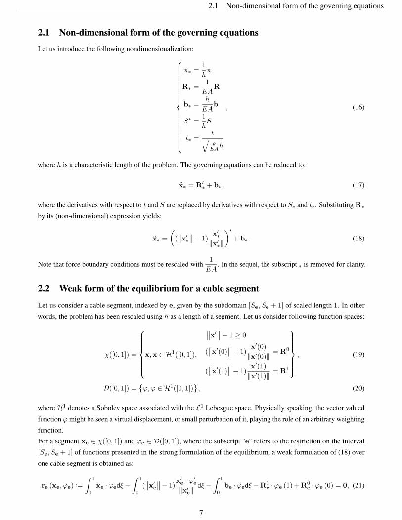
2.2 Weak form of the equilibrium for a cable segment

Let us consider a cable segment, indexed by e, given by the subdomain [Se, Se + 1] of scaled length 1. In other

words, the problem has been rescaled using h as a length of a segment. Let us consider following function spaces:

χ([0, 1]) =

x,x ∈ H1([0, 1]),

∥∥x′∥∥− 1 ≥ 0

(∥∥x′(0)

∥∥− 1)x′(0)

‖x′(0)‖ = R0

(∥∥x′(1)

∥∥− 1)x′(1)

‖x′(1)‖ = R1

, (19)

D([0, 1]) =ϕ,ϕ ∈ H1([0, 1])

, (20)

whereH1 denotes a Sobolev space associated with the L1 Lebesgue space. Physically speaking, the vector valued

function ϕmight be seen a virtual displacement, or small perturbation of it, playing the role of an arbitrary weighting

function.

For a segment xe ∈ χ([0, 1]) and ϕe ∈ D([0, 1]), where the subscript "e" refers to the restriction on the interval

[Se, Se + 1] of functions presented in the strong formulation of the equilibrium, a weak formulation of (18) over

one cable segment is obtained as:

re (xe, ϕe) :=

∫ 1

0xe ·ϕedξ +

∫ 1

0(∥∥x′e∥∥− 1)

x′e · ϕ′e‖x′e‖

dξ −∫ 1

0be ·ϕedξ −R1

e ·ϕe (1) +R0e ·ϕe (0) = 0, (21)

7

for all ϕe ∈ D([0, 1]) and xe ∈ χ([0, 1]). The notation R1e and R0

e respectively stand for the internal forces at the

right end and left end segment e. The global equilibrium is obtained by summing the contribution of each segment

such that:

0 =N∑e=1

re (xe, ϕe) . (22)

Assuming that ϕ is continuous at connected nodes (i.e. ϕe+1 (0) = ϕe(1)), the jumps of internal forces appear in

the assembled problem as:

−p =N∑e=1

[R0

e · ϕe (0)−R1e · ϕe (1)

](23)

= R01 · ϕ1 (0) +

N−1∑e=1

[R0

e+1 · ϕe+1 (0)−R1e · ϕe (1)

]−R1

N · ϕN (1) (24)

=(R0

1 − 0)· ϕ1(0) +

N−1∑e=1

[(R0

e+1 −R1e

)· ϕe+1(0)

]+(0−R1

N

)· ϕN (1) (25)

=N∑e=1

[−p0

e · ϕe(0)]− p1

N · ϕN (1). (26)

p0e denotes for the applied point force on the left end of segment e.

3 Method 1: Standard FEM and spurious solutions

Provided (21) and (22), a nonlinear finite element can be formulated for the cable problem.

3.1 Finite element approximation

In order to build a discrete approximation of our system, the approximation is written for one arbitrary element

indexed by e as :

xe ≈ N(ξ)Xe, (27)

ϕe ≈ N(ξ)Φe, (28)

x′e ≈ N′(ξ)Xe, (29)

ϕ′e ≈ N′(ξ)Φe, (30)

where Xe ∈ IRne are the nodal unknowns and N(ξ) ∈ IR3×ne is the shape function matrix. The variable ξ ∈ [0, 1]

is the non-dimensionnal variable of the interpolating function used to approximate the restriction Xe and we

introduce the following notation:

B(ξ) = N′(ξ)>N′(ξ). (31)

8

3.2 Equality constraints for prescribed node positions

Let us apply this discretization to the residual re in (21). To make the derivations concise, we split the calculation

term by term: ∫ 1

0xe · ϕedξ ≈ Φ>e

[∫ 1

0N>N dξ

]Xe, (32)∫ 1

0

((∥∥x′e∥∥− 1)

x′e‖x′e‖

)· ϕ′edξ ≈ Φ>e

[∫ 1

0

(1− 1√

X>e BXe

)B dξ

]Xe, (33)∫ 1

0be · ϕedξ ≈ Φ>e

[∫ 1

0N>be dξ

]. (34)

Equations (32 - 34) define respectively the elementary mass matrix (Me), the elementary rigidity matrix (Ke(Xe)),

the elementary body force vector (be) and the point efforts vector (pe) is obtained via (26) i.e.:[∫ 1

0N>N dξ

]= Me, (35)[∫ 1

0

(1− 1√

X>e BXe

)B dξ

]= Ke(Xe), (36)[∫ 1

0N>be dξ

]= be, (37)[

p0e, 0, . . . , 0

]>= pe , e 6= N, (38)[

p0N , 0, . . . , 0,p

1N

]>= pe , e = N, (39)

Then for each element we have the following expression for re:

MeXe + Ke(Xe)Xe − be − pe = 0. (40)

The elementary tangent stiffness matrix may be derived considering the gradient of the following quantity:

∂

∂Xe(Ke(Xe)Xe) = Ke(Xe) +

∫ 1

0

(1√

X>e BXe

)3

BXeX>e B dξ

= ∆Ke(Xe). (41)

The latter can be assembled into the global tangent stiffness matrix ∆K through the same assembly process than

before.

3.2 Equality constraints for prescribed node positions

The local discrete equation of motion given by (40) can be assembled to obtain a global system with the following

form:

0 = MX + K(X)X− b− p. (42)

As we are manipulating a nonlinear problem, direct substitution of imposed node-position may be numerically

difficult and not practical when it comes to impose more than end-node positions (e.g. presence of intermediate

support).

9

3.3 Non-admissible numerical solutions for the static analysis of the hanged cable

We propose an approach based on Lagrange multipliers associated with equality constraints:0 = MX + K(X)X− b− p−A>λ,

0 = AX− c,(43)

where the matrix A ∈ IR3(N+1)×3m where m ≥ 1 is the number of imposed node positions. The vector A>λ is the

reaction forces due to the constraints.

The matrix A selects the degrees of freedom (dofs) that are imposed to c), producing a force as a response λ.

the method described in section 3 will be now denoted as "Method 1" which consists in a canonical finite element

approach to the cable problem.

3.3 Non-admissible numerical solutions for the static analysis of the hanged cable

A particular application case of (43) is the static response of a cable under self-weight loading. As analytic solution

of such system is known, then comparisons with the obtained numerical solution and the sought equilibrium can be

performed. In this article, we used a simple linear interpolation given by:

N(ξ) =

1− ξ 0 0 ξ 0 0

0 1− ξ 0 0 ξ 0

0 0 1− ξ 0 0 ξ

, Xe =

x1

y1

z1

x2

y2

z2

, (44)

but the results are equivalent with higher order approximations. Numerical solutions for the statics of the cable

under its self-weight are obtained with Newton method by solving r(X, λ) = 0 with:

r(X, λ) =

K(X)X− b− p−A>λ,

AX− c.(45)

The Jacobian matrix of this problem reads as:

J = ∇>(X,λ) [r(X, λ)] =

[∆K(X) −A>

A 0

]. (46)

In practice, the Jacobian matrix for cable is ill-conditioned and the conditioning of the problem strongly depends on

the following parameter:

α =ρgh

EA, (47)

where h is the size of one element i.e.L

N. The bigger α is, the more accurate and easier the computation is.

However, many civil engineering applications correspond to very small value of the α parameter. Moreover, we see

that the finer the mesh is, the worse is the conditioning which means that precision of the results is obtained with

more numerical efforts. This cause issues on numerical equilibria obtained via the finite element approach.

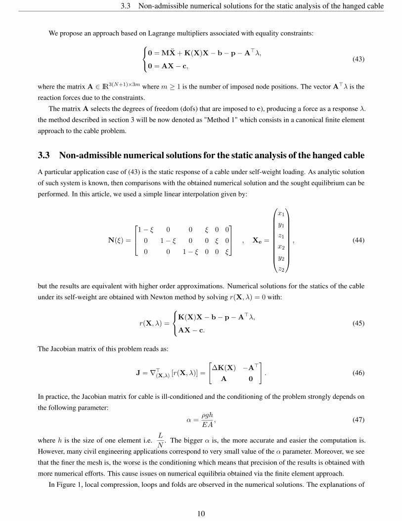
In Figure 1, local compression, loops and folds are observed in the numerical solutions. The explanations of

10

3.4 Further discussion about the existence of non admissible cable equilibria

a b

x

y

x

y

c

x

y

Figure 1: Results obtained from standard FEM modelling of the cable: a creation of a loop; b zoom at one loop ofa ; c creation of compression and folds for a cable (solid line ) with end nodes imposed ( )

these non admissible solutions rely on two facts: a) the non-compression condition given by (5) is not enforced by

the mathematical model, and b) the problem is badly conditioned leading to convergence problems in the Newton

iterations. As a consequence, expecting the self-hanging cable configuration as the only possible output is hazardous.

To ensure the numerical solutions to converge to a tensile state, we must complete the model to ensure that the strain

is positive ε ≥ 0. This will be the key points of the contribution of this paper in the remaining parts of the article.

3.4 Further discussion about the existence of non admissible cable equilibria

Taking a look at (11), the following assumptions are made:

• ε may exhibit jumps.

11

a b

x0 [|ε|] xL-1

0

1

yε>0

yε<0

260 × ε

260 × ε

x

y

x0 [|ε|]2 [|ε|]1 xL-1

0

1

yε>0

260 × ε

yε<0

260 × ε

yε>0

360 × ε

x

yFigure 2: Analytically obtained profiles of a cable with corresponding dilatation where the positiveness of ε is

removed from assumptions. Cable may exhibit tensed segments (solid line ) or compressed segments (solid line)

• ε may be negative, but still verifies continuum mechanics assumptions (ε > −1).

As discussed earlier, it is possible that the solution converges to a state with compressive strains. It can be shown

that equilibria corresponding to the coexistence of compressed and tensed segments satisfy the local equilibrium

given by (42). For a self-hanging cable, it consists of finding a continuous profile with a jump in the axial stress. As

soon as the positiveness assumption of ε is removed from the equations, the uniqueness of the cable profile is lost

and compressed segment may exist. This observation is corroborated in [26] where cables are shown to exhibit a

switch between hogging and sagging configurations through the iterative process.

In Figure 2, analytical solutions with continuous or discontinuous internal forces are illustrated. Those solutions

correspond to a minimum of energy related to a local equilibrium given by (11) and therefore a zero of the residual

equation (45). From these examples, the so called “spurious” solutions can be spotted in the form of local minima

that violate the pure tensile behavior assumption. The amounts of potential energy for these two-solutions can be

derived and shown to be bigger than the one of tensile catenary solutions with same length. In other terms, these

solution corresponds to local extrema of the potential energy.

From the engineering point of view, these spurious solutions must be avoided. From a theoretical point of view,

they are, most of the time, unstable solutions. When computing closed form solutions, it is rather easy to avoid

them. The goal is now to propose a numerical method to compute only tensile solutions, suppressing the spurious

solutions.

4 Method 2: A modified finite element formulation for cables

As discussed in Section 3, the standard formulation and its finite element procedure suffer of two drawbacks:

• the model and the finite implementation provide us with non admissible solutions with compressive strains,

12

4.1 Axial forces reformulation and modified gradient

• it is highly sensitive to ill-conditioned matrices, so it needs to be improved in order to compute accurate

solutions with a finer mesh.

The proposed approach modifies the non-dimensional system of equations by correcting the stiffness matrix. Key

concepts and validity of these modifications are mainly inspired by the work of Kanno and Ohsaki [11]. The

proposed Algorithm 1 allows to compute admissible tensile solutions without an a priori knowledge of the solutions,

of the definition of a specific loading sequence, or suitable initial guesses or numerical regularization of the tangent

matrix via Levenberg-Marquardt method [20]. If the cable is assumed to only produce tensile forces, it means that

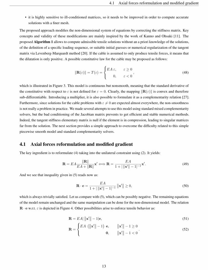
the dilatation is only positive. A possible constitutive law for the cable may be proposed as follows:

‖R(ε)‖ = T (ε) =

EA ε, ε ≥ 0

0, ε < 0, (48)

which is illustrated in Figure 3. This model is continuous but nonsmooth, meaning that the standard derivative of

the constitutive with respect to ε is not defined for ε = 0. Clearly, the mapping ‖R(ε)‖ is convex and therefore

sub-differentiable. Introducing a multiplier, it is also possible to formulate it as a complementarity relation [27].

Furthermore, since solutions for the cable problems with ε 6= 0 are expected almost everywhere, the non-smoothness

is not really a problem in practice. We made several attempts to use this model using standard mixed complementarity

solvers, but the bad conditioning of the Jacobian matrix prevents to get efficient and stable numerical methods.

Indeed, the tangent stiffness elementary matrix is null if the element is in compression, leading to singular matrices

far from the solution. The next section provides a simple approach to overcome the difficulty related to this simple

piecewise smooth model and standard complementarity solvers.

4.1 Axial forces reformulation and modified gradient

The key ingredient is to reformulate (4) taking into the unilateral constraint using (2). It yields:

R = EA‖R‖

EA+ ‖R‖x′ ⇐⇒ R =

EA

1 + | ‖x′‖ − 1|−1x′. (49)

And we see that inequality given in (5) reads now as:

R · e =EA

1 + | ‖x′‖ − 1|−1∥∥x′∥∥ ≥ 0, (50)

which is always trivially satisfied. Let us compare with (5), which can be possibly negative. The remaining equations

of the model remain unchanged and the same manipulation can be done for the non-dimensional model. The relation

R · e w.r.t. ε is depicted in Figure 4. Other possibilities arise to enforce tensile behavior as:

R = EA|∥∥x′∥∥− 1|e, (51)

R =

EA(∥∥x′∥∥− 1

)e,

∥∥x′∥∥− 1 ≥ 0

0,∥∥x′∥∥− 1 < 0

. (52)

13

4.1 Axial forces reformulation and modified gradient

ε

T

Figure 3: Non-smooth formulation of constitutive law of (48)

-1 0 1

ε

R · e

Figure 4: Relation between R · e and ε; Usual case presented in (4) (dashed line ) ; Proposed approach provided in(50) (solid line ) ; The rheology given by (51) (dotted line ) ; The rheology given by (52)(solid line )

14

4.2 finite element approximation and modified Jacobian matrix

4.2 finite element approximation and modified Jacobian matrix

The problem will be approximated via a finite element approach using this new behavior law (49). The main changes

rely on the computation of the stiffness matrix and the tangent matrix and leads to:[∫ 1

0

1

1 + |√X>e BXe − 1|−1

B dξ

]= Ke(Xe). (53)

The tangent matrix needs the computation of differential for a nonsmooth function. Since the stiffness matrix in

(53) is piecewise continuous but not differentiable at√

X>e BXe−1 = 0, we compute an element of the generalized

Jacobian:

He(Xe) ∈ ∂Xe (Ke(Xe)Xe) = ∂Xe

[∫ 1

0

1

1 + |√

X>e BXe − 1|−1B dξ

](54)

as:

He(Xe) = Ke(Xe) + Ke(Xe), (55)

where:

Ke(Xe) =

∫ 1

0

(1

|√X>e BXe − 1|+ 1

)2sgn(

√X>e BXe − 1)√X>e BXe

BXeX>e B dξ

, (56)

where sgn(√

X>e BXe − 1) is the sgn function defined in (12 ) applied to√X>e BXe − 1. As outlined before, the

term√

X>e BXe − 1 is assumed to be different from 0 almost everywhere if a body load is applied. Using another

value of the generalized Jacobian at√X>e BXe − 1 = 0 does not change the computed solution at convergence.

In order to remain as general as possible, each integral needed in the computation shall be approximated via

Gauss point quadrature [28] as:

Ie =

∫w(ξ)f(ξ) dξ ≈

n∑i=1

Hif(ξi). (57)

In the problem presented here, an exact result can only be obtained if the interpolation is linear. However, the

presented methodology is adaptable for an arbitrary quadrature. This approach, once implemented in FEM, still

produces numerical solutions with compressed segments. For that reason, we will propose some hints to compute a

purely tensile behavior of a cable system in the next section.

4.3 Numerical hints: Methods 3 & 4

We saw that methods 1 and 2, respectively the canonical FEM implementation and the one given by (49), fail to

provide with a purely tensed configuration at rest

To improve efficiency and reduce the number of iterations, we propose the algorithm given in Algorithm 1. The

latter enforces the iteration to be in tension only by ensuring the global gradient J to give the direction of a tensile

configuration. The script works as an active/passive elastic law forcing the system to create elastic energy coming

from a fully tensed configuration. It can also be viewed as a generalized Newton technique or an active set strategy

[29]. To improve convergence when we are far from a tensile solution, using a modified Jacobian procedure which

origin comes from [11]. We chose to de-activate the compression contribution from the system equation when the

iterations are compressed locally, which corresponds to the rheology described in (48). However, it follows that the

Jacobian will be singular. To overcome the singularity we choose to set the gradient to the one of system which

15

4.4 Numerical examples

corresponds to rheology given in (49) which ensure a descent towards a tensed state.

Let us define, for an arbitrary element e, the current length as

le =

∫ 1

0

√X>e BXe dξ, (58)

The non-smooth iteration process can be described as follows for an element:

• If element e is working strictly in tension, i.e. le > 1, we use the expression of re and He(Xe) provided in

(21) and (55) respectively

• If element e is working in compression, i.e. le ≤ 1, we use modified expressions of re and ∆K(Xe) provided

in (59) and (60) using

r∗e = −be + pe. (59)

Here is kept the part of the Jacobian matrix which ensures the current element force to be positive (see (50).

This method regularizes the iteration since it avoids the singularity in the Jacobian.

∆K∗e(Xe) = Ke(Xe) =

[∫ 1

0

1

1 + |√

X>e BXe − 1|−1B dξ

](60)

Adding the equality constraints, the static equilibrium is computed via:(X0, λ0) ∈ IRN

(Xk+1, λk+1) = (Xk, λk)− J [f∗(Xk, λk)]−1 r∗ (Xk, λk)

, (61)

where J denotes the tangent matrix obtained by assembling the contribution of tangent matrix and the contribution

of the constraints given by the matrix A.

This procedure dictates numerically the system to balance efforts with purely tensile forces which is physically

understandable due to the impossibility for a cable to resist to compression. This avoids spurious solutions quoted

by Felippa [20]. Moreover, this procedure allows to avoid also a guess which is almost the solution (which is not

feasible for complicated systems) and do not use Levenberg-Marquardt methods where damping parameters has to

be chosen carefully [20].

We can also benchmark with 2 other methodologies denoted as:

• Method 3: FEM implementation using (59), (55) and (61)

• Method 4: Implementation of (52) with the same spirit than Method 3 (de-activation and modified gradient)

All the proposed methods will be used for performance comparisons of each implementation (see section 4.5).

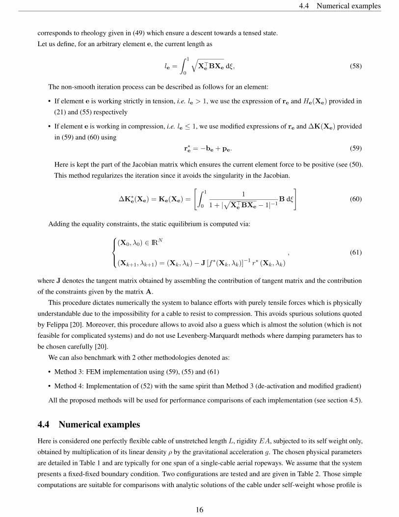
4.4 Numerical examples

Here is considered one perfectly flexible cable of unstretched length L, rigidity EA, subjected to its self weight only,

obtained by multiplication of its linear density ρ by the gravitational acceleration g. The chosen physical parameters

are detailed in Table 1 and are typically for one span of a single-cable aerial ropeways. We assume that the system

presents a fixed-fixed boundary condition. Two configurations are tested and are given in Table 2. Those simple

computations are suitable for comparisons with analytic solutions of the cable under self-weight whose profile is

16

4.4 Numerical examples

Algorithm 1 Finite element procedure for the statics of cable (Modified Newton-Raphson method)Require: EA ≥ 0, ρ ≥ 0, x0, xL, b , p ∼ applied jumpsRequire: N , maxiter, tolh← L

N; b∗ ← h

EAb; j∗ ← 1

EAj ; c← 1

h(x(0), x(L))>

# Build a stretched rope of length(1 + ρgh

EA

)starting at 1

hx0 with n+ 1 nodes and directed by xL−x0

‖xL−x0‖X← build_initial_condition (x0,xL, h, n, ρ, g, , EA)A← build_constraints_matrix()λ← 0test← +∞ ; niter ← 0while test ≥ tol and niter < maxiter dor← 0J← 0# FE Matrix assemblyfor e = 0 : n− 1 do

# With integrals approximated with Gauss pointsXk ← dof_element(X, e)if le ≥ 1 thenre ← re + Ke(Xk)Xk

Je ← Je + Ke(Xk)elsere ← 0Je ← Je + Ke(Xk)

end ifbe ← compute_body_load(e)pe ← compute_punctual_load(e)r← assemble_residual(re)JXX ← assemble_Jacobian (Je)

end for

# Equality constraints

r←(r−A>XAX− c

)J←

[J −A>A 0

](X, λ)> ← (X, λ)> − J−1r # Linear system solvingtest← ‖r‖; niter ← niter + 1 # Update criteria and iterates

end whilereturn X, λ

17

4.4 Numerical examples

EA (MPa) L (m) ρ (kg.m−1) g (kg.s−2)40 51 4 9.81

Table 1: Parameters used for calculations of the rest positions of a fixed-fixed cable

x(0) x(L)dofs x0 y0 z0 xL yL zL

Case 1 0 0 0 50 0 0Case 2 0 0 0 50 8 0

Table 2: Boundary conditions used for calculations of the rest positions of a fixed-fixed cable

given by the elastic catenary equations [16]:

x(S) = xL −H

EA(L− S)− H

ρgln

ρgL+ V +√H2 + (ρgL+ V )2

ρgS + V +√H2 + (ρgS + V )2

, (62)

y(S) = yL −(L− S)

2EA(2V + ρg (L+ S))− 1

ρg

(√H2 + (ρgL+ V )2 −

√H2 + (ρgS + V )2

), (63)

obtained from (13)-(14) where B is set to zero.

This allows to estimate the error made by the finite element approximation. A mesh with 300 elements starting

from an arbitrary configuration is used. In the examples, a initial configuration has been set to a straight line with

an initial dilatation to avoid singularity of the stiffness matrix at the first iteration. The problem remains stiff,

but spurious solutions obtained from total Lagrangian bar elements or linear bar element [20] are avoided with a

relatively good agreement with the analytic solution. Despite the low order-element used there, the nonsmooth

elastic model allows to compute strain profiles that are positive which is an improvement of standard FEM structural

analysis of cables. The comparison with respect to the analytical solution is illustrated in Figure 5. We see that the

error value is order 10−5 or less. This improves standard FEM methods applied to cable problems where the error is

usually at the order 10−1 ∼ 10−3 [14].

All parameters of the system which are used are depicted in Appendix A.

4.4.1 Effects of the rigidity

The effect of the rigidity on the mid-span deflection can be studied without any issues with the proposed approach.

We see that the proposed approach allows to converge to the solution of an inextensible cable when EA→∞, and

that the sag of the cable (measured at mid-span in the vertical direction) appears to be exponentially decreasing with

the rigidity. The elasticity may be neglected for the computation of static profile when EA is large as depicted in

Figure 6.

In this section we compute the equilibrium for every cables which parameters are similar to those given in Table

1. However the rigidity, EA, is taken to be variable and we observe its relationship with the midspan deflection.

Here EA spreads from 15 kPA to 10 GPa, the latter is to be considered as an "infinite rigidity".

4.4.2 Effects of point loads

Using the cable parameters depicted in Table 1 and boundary conditions given in Table 3, loads applied are all the

18

4.4 Numerical examples

a b

x0 x xL

y0 = yL

y

x0 x xL

y0

yL

y

Figure 5: Rest configuration of an aligned cable a (FEM error = 1e−5) and inclined cable b (FEM error = 7e−8)obtained via FEM (solid line ) and obtained analytically (dashed line )

x0 xL

y0 = yL

Evolution of cable sag

EA [kPa]

15

∞

5 6 7 80

5

10

15

log10 (EA)

−ymid

Figure 6: Rest configuration of a cable with respect to the case 1 obtained by FEM with rigidity EA varying from 1kPA to 1 GPA (left); Evolution of mid-span deflection with the logarithm of cable rigidity, log (EA) (right)

x(0) x(L)dofs: x0 y0 z0 xL yL zL

Case 1 and 3 0 0 0 50 0 0Case 2 0 0 0 50 10 0

x(0) Point load at S = Ldofs: x0 y0 z0 x direction y direction z direction

Case 4 0 0 0 10000 0 0

Table 3: Boundary conditions used for calculations of the rest positions of a cable subjected to point loads

same and are chosen for the example asρLg

3.

19

4.4 Numerical examples

The results depicted in Figure 7 show that our approach allows to keep the catenary shape of the cable profile

without any compression and it asymptotically converges to the assembly of taut string elements when the point

loads are significantly large with regards to the cable weight. In the cases 1 and case 2, the cables are loaded with

descending point loads and cases 3 and 4 the cable is loaded with ascending point loads which respectively may

correspond to cabin loads or support reaction. The jumps in internal forces are successfully caught, and the method

proposed is efficient to compute a slope discontinuity.

Downward point loads

a b

x0 xL

y0 = yL

x0 xL

y0

yL

Upward point loads

c d

x0 xL

y0 = yL

x0 xL

y0

Figure 7: a Cable at rest (solid line ) subjected to downwards point loads at given positions ( ) for aligned andb inclined cable obtained by FEM / c Cable at rest (solid line ) subjected to upwards point loads ( ) for an

aligned cable and an d imposed end-force cable obtained by FEM

20

4.5 Heuristic convergence study

4.5 Heuristic convergence study

The convergence of the proposed method is detailed here in four parts. First, a performance profile of methods 1 to

4 is given which proves that our proposed approach is more robust to compute solution for cable problem. Then, the

accuracy of solution with regard to the mesh is discussed. Then, the quadratic convergence of the modified Newton

approach is shown. Eventually some observations about the influence of the α parameters on problem conditioning

is provided.

4.5.1 Performance profiles

Here we use the methodology proposed in [30] to compute comparisons of the robustness of the proposed approach

compared to a standard FEM implementation. All four methods are used to compute a solution to p ∈ N identical

problems (for instance with increasing number of elements or changing parameters). According to a performance

criterion defined by:

critp,s = nit + nε<0 ×maxiter ; s = 1, 2, 3, 4. (64)

nε<0 stands for the number of compressed element in the system. A performance ratio can be defined for each

method and problem as:

rp,s =critp,s

min(critp,s, s = 1, 2, 3, 4). (65)

To have an overall assessment of the performance of each method according to the criterion (64), we define the

following:

ρs(τ) =1

pcard (p∗, rp∗,s ≤ τ) . (66)

The quantity ρs(τ) corresponds to the probability that the performance ratio of the method s is within a factor τ of

the best possible method. A general benchmark methodology for different numerical methods (or different solvers)

is detailed in [30] and objectively describes the major performance characteristics of an algorithm with regards to an

efficiency metric.

Let us remember that:

• Method 1: Classic FEM implementation of governing equation

• Method 2: FEM implementation of governing equation where rheology has been substituted for (49)

• Method 3: FEM implementation of (55),(59) and (61) associated to (49)

• Method 4: FEM implementation of (55),(59) and (61) associated to (52)

In our work, we choose to consider the number of compressed elements as penalties for the efficiency since it

produces wrong evaluation of tension and static profiles with folds and knots. Moreover, the number of iterations is,

in a first approach, suitable to account for computation effort since every method relies on Newton iterations. Figure

8 depicts the relative performance of each method. The intrinsic efficiency of each method can be seen at ρs(1)

which gives the proportion of problems solved by method s with the same iteration count than the fastest method.

We see that the proposed methods 3 and 4 are the best choices to compute robust solutions at given tolerance without

any compression within a few numbers of iterations. Moreover, the canonical approach struggles to provide an

acceptable result and that it cannot compete with the proposed approach in terms of number of iterations. Our

proposed algorithm is robust since it solves all the problems. Note that Method 1 only solves 90% of the problems,

although it is a very simple configuration. The Method 2 is proven to be totally inefficient to overcome compression

21

4.5 Heuristic convergence study

a b

1 1.5 2 2.5 3

0

0.1

0.2

0.3

0.4

0.5

0.6

0.7

0.8

0.9

1

: Method 1: Method 2: Method 3: Method 4

τ

ρs(τ )

1 1.5 2

0

0.1

0.2

0.3

0.4

0.5

0.6

0.7

0.8

0.9

1

: Method 1: Method 2: Method 3: Method 4

τ

ρs(τ )

Figure 8: Performance profiles according to iteration count of the described methods in the paper at tolerancetol = 10−8 for an aligned configuration which parameters are used in figure 1 with increasing number of element a

and for CPU-time b

in the iteration process. The piecewise linear constitutive law (52) cannot be successfully used since singular

Jacobian matrix occurs as soon as one single segment of cable is compressed. The same comparison can be endowed

with CPU-time instead of the number of iterations to account for the relative computational time needed to obtain a

satisfying solution, see Figure 8. To this purpose, we use the methodology of Dolan and More [30] as developped in

their work with a penalty for the solutions with compression:

tp,s = CPU-timep,s + ∃ε < 0 ×∞ ; s = 1, 2, 3, 4. (67)

∃ε < 0 returns 1 if there is any compressed segment or 0 if not. We take the convention that 0×∞ = 0 in this time

computation.

A performance ratio can be defined for each method and problem as:

r∗p,s =tp,s

min(critp,s, s = 1, 2, 3, 4). (68)

Then performance reads:

ρ∗s(τ) =1

pcard

(p∗, r∗p∗,s ≤ τ

). (69)

With the CPU-time comparison, the combination of convergence speed and accuracy is confirmed. Indeed, even

if proposed methods are slightly slower due to conditional expressions in the iteration process, the robustness of

the mentioned approaches are clearly shown. Only the speed of computation is used as a performance metric,

under the condition that the solution exhibits only tensed segments. In this case, the performance of the methods 3

and 4 are proven to be the best for further calculations with an intrinsic , which is overwhelming the naive FEM

implementation and the implementation of (49).

22

4.5 Heuristic convergence study

a b

0 1 2 3 4

-1

0

1

2

3

-x

-2x

log10(N)

log 1

0(er

r)

0 1 2 3 4

-1

0

1

2

3

-x

-2x

log10(N)

log 1

0(er

r)

Figure 9: Computation of the numerical error with respect to (70) with a α = 1N× 1, 1.10−4 and b

α = 1N× 1, 02.10−1. N is the number of elements in the mesh

4.5.2 Convergence with respect to mesh size

Regarding to two different sets of physical parameters, the convergence of the numerical solution is studied. By the

term “convergence”, we mean that the error between the exact solution and the numerical one is quantified via:

err =

√∫ L

0(x(S)− xnum)2 dS ≈ L

Nf

√√√√n+1∑k=0

((x(Sk)− xnum(Sk))2, (70)

where for the numerical solution we use the interpolation function to estimate xnum(Sk) and x is the analytic cable

profile given by (13)-(15) and Nf is the number of cable segment in the converged state. To make fair comparisons,

we used the same number of evaluation points for every mesh. It is noticeable that precision increases with the

number of elements (see Figure 10) which was not the case before introducing the standard FEM strategy (61).

Moreover, first insights about the importance of α for the conditioning is given here. For the same boundary

conditions and meshes, the final accuracy is better when α is large as depicted in figure 9. The ill-conditioned

matrices of the iterative process have been improved but is still present, causing a lost of the quadratic rate of

convergence for fine mesh. The use of non-dimensional problem allows to decreases conditioning, however, it will

remain impossible to totally overcome it due to the nature of the problem.

For aerial cable ropeways, the values of α are small and we are near to the inextensible case. The conditioning

causes problems of rate of convergence, but the numerical method is able to give a robust solution with a reasonable

accuracy.

4.5.3 Quadratic convergence of Modified Newton iterations

The quadratic convergence of Newton’s iteration is tested. It is numerically shown that for a few elements, the

quadratic convergence is retrieved and that tolerance level is satisfied. However, when the number of elements

23

x

y

Figure 10: Evolution of the cable profile with N = 3 (solid line ) , N = 6 (solid line ) , N = 12 (solid line) and N = 1536 (solid line ) . Nodes are indicated by bullets when their number is low

increases, the norm of the residual equation reaches a threshold which appears to be function of system conditioning

(Figure 11). As far as this threshold is acceptable, the stopping criteria may be modified taking into account the

length of the Newton step to avoid perpetual iterations. However, the methods appear to remain quadratic despite

the implemented non-smooth constitutive law. The threshold tends to increase with the number of elements, using

this fact, some loop conditions may be implemented to accelerate computational time with, for instance, a test on

the relative evolution of the norm of the residual equation.

4.5.4 Evolution of problem conditioning with regard to α

We recall the following parameter expression:

α =ρgh

EA=

ρgL

EA N. (71)

Two key parameters enter in the discussion: the first one is the physical ratioρgL

EAand the second one is the number

of elements N . The conditioning of the Jacobian matrix can be depicted with respect to those two parameters.

As expected, this matrix becomes ill-conditioned as soon as the amount of element increase or when the weight

becomes small compared to the cross section rigidity as shown in Figure 12. It seems that we must have more

elements in the model in order to have a good estimation of the tension, however the threshold of the converged

residual decreases while the number of elements increases which is counterintuitive for the finite-element procedure.

5 Validation of the proposed method on applications

5.1 Static analysis of cable networks

Numerically speaking, cable network analysis is a challenging task. As the statics of one single cable is already

challenging to compute by the finite element approach, cable networks analysis via finite elements are subjected

to a lot of numerical issues [20]. Some of these issues have been addressed with the implementation of "catenary

24

5.1 Static analysis of cable networks

a b

1 3 5 7 9 11 13 15 17 19 21

-15

-12

-10

-5

0

5

-x2

N = 3 :N = 6 :N = 12 :N = 24 :

niter

log 1

0‖r‖

1 3 5 7 9 11 13 15 17 19 21

-15

-12

-10

-5

0

5

-x2

N = 48 :N = 96 :N = 192 :N = 384 :

niter

log 1

0‖r‖

c

1 3 5 7 9 11 13 15 17 19 21

-15

-12

-10

-5

0

5

-x2

N = 4768 :N = 1536 :N = 3072 :

niter

log 1

0‖r‖

Figure 11: Evolution of the norm of the residual equation (and equality constraints) with regard to the number ofiteration for a N = 3 to 24 elements, b N = 48 to 384 elements and c N = 768 to 3072 elements

elements” [12, 21, 23], then the efficiency of these methods can be compared with an assembled finite element

problem derived from (45) with our proposed method. Cables are assembled with bilateral constraints applied on

specific elements. Then the statics of a cable network are obtained as follows:0 =K(X)X− b− p−A>λ− A>λ

0 =AX− c

0 =AX

, (72)

where the A matrix accounts for the connection between the dofs of the global system, in other words, it is the

incidence matrix of the network. The A matrix should be a full rank matrix. To ensure this condition, a Gram-

Schmidt procedure is endowed. New matrices and system variables are simple concatenation of isolated cables

25

5.2 Modal analysis

a b

4 5 6 7 8 9 100

2

4

6

8

log10(EA)

log10

cond

(J)

0 1 2 30

2

4

6

8

log10(N)

log10

cond

(J)

Figure 12: Evolution of the conditioning (log10) of the Jacobian matrix with regard to a the weight/rigidity ratio andwith regard to b the number of elements

composing the overall system. The matrix A selects the dofs subjected to a fixed boundary condition. The vector λ

contains the Lagrange multipliers associated with the boundary conditions and λ houses the Lagrange multipliers

associated to the connection between 2 nodes. The procedure has been applied to the statics of a spider web so that

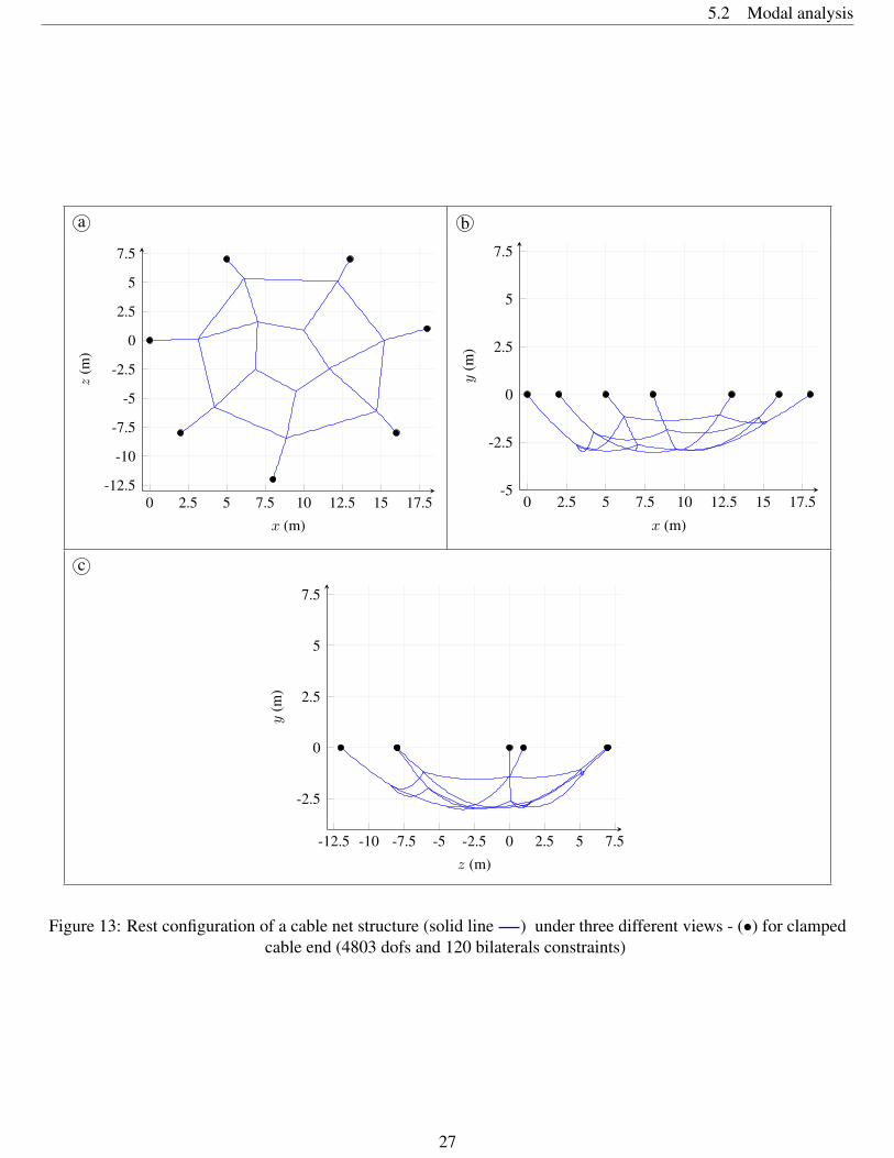
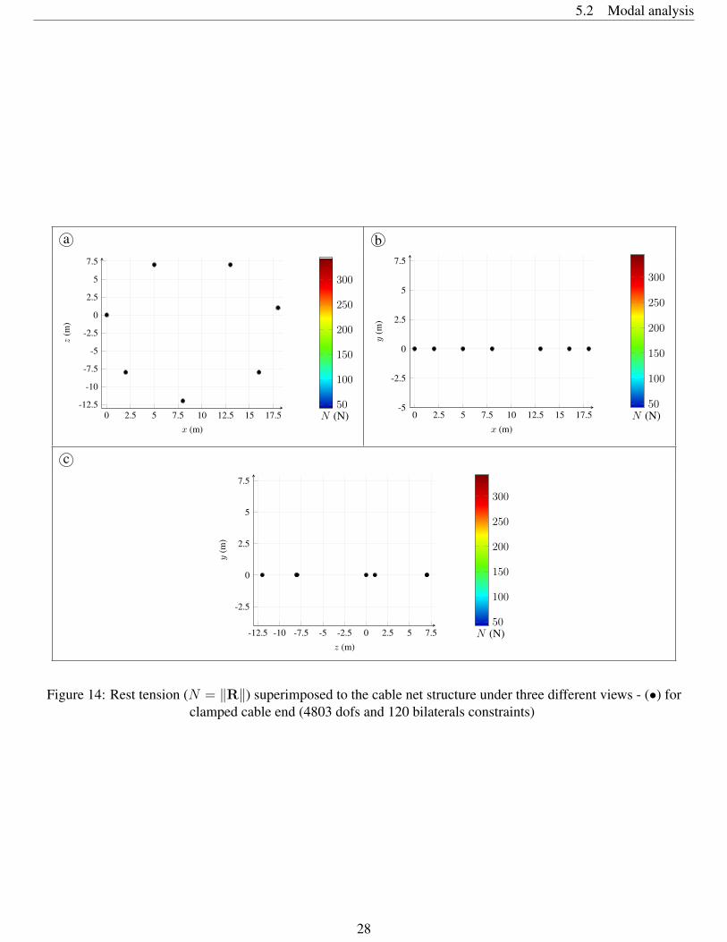
the rest configuration and the tension profile at rest can be depicted (see Figures 13 and 14). This 3D-equilibrium

has been satisfied in 40032 iterations at res= 6.84 × 10−7. The final descent direction was nearly zero, indeed

‖δ‖ = 1.79× 10−13 so that the equilibrium is considered accurate.

5.2 Modal analysis

Let us consider the linearized dynamics of a fixed-end cable. Various approaches have been used such as considering

the elastic linear vibrations, given by increment U, around the rest configuration, often referred as “static configura-

tion” [2, 3]. The dynamics sought is a linear (and relatively small) around the hanged profile. This is equivalent to

seek for the eigenvalues and eigenvectors of the tangent stiffness matrix computed from the rest configuration [18].

After some manipulation on the non-dimensional system (43), it is equivalent to solve the following eigenvalue

problem: (M−1∆K(X) + aI

)Ua = 0. (73)

In this case the scalar a is often a pure complex so that a = −Ω2 and Ω physically corresponds to the frequencies

of the system while Ua = Uω is the associated modal displacement vector. Similar methods can be applied for

damped system which are classified in [31].

5.2.1 Application to the mode shapes finding of a particular cable

Solving (73) for the cable with mechanical properties given in Table 1 allows to compute its modal characteristics.

Interestingly, it is obtained that the modes are in (x, y)-plan or in the (x, z)-plane. They respectively stand for

26

5.2 Modal analysis

a b

0 2.5 5 7.5 10 12.5 15 17.5-12.5

-10

-7.5

-5

-2.5

0

2.5

5

7.5

x (m)

z(m

)

0 2.5 5 7.5 10 12.5 15 17.5-5

-2.5

0

2.5

5

7.5

x (m)

y(m

)

c

-12.5 -10 -7.5 -5 -2.5 0 2.5 5 7.5

-2.5

0

2.5

5

7.5

z (m)

y(m

)

Figure 13: Rest configuration of a cable net structure (solid line ) under three different views - (•) for clampedcable end (4803 dofs and 120 bilaterals constraints)

27

5.2 Modal analysis

a b

0 2.5 5 7.5 10 12.5 15 17.5-12.5

-10

-7.5

-5

-2.5

0

2.5

5

7.5

x (m)

z(m

)

50

100

150

200

250

300

N (N) 0 2.5 5 7.5 10 12.5 15 17.5-5

-2.5

0

2.5

5

7.5

x (m)

y(m

)

50

100

150

200

250

300

N (N)

c

-12.5 -10 -7.5 -5 -2.5 0 2.5 5 7.5

-2.5

0

2.5

5

7.5

z (m)

y(m

)

50

100

150

200

250

300

N (N)

Figure 14: Rest tension (N = ‖R‖) superimposed to the cable net structure under three different views - (•) forclamped cable end (4803 dofs and 120 bilaterals constraints)

28

5.2 Modal analysis

planar and out-of-plane mode, see Figure 15. Of course, this partitioning will not be valid for a cable network where

an absence of alignment will destroy this property.

Modes are depicted with regards to the reference curvilinear abscissa. We see here that FEM allows to catch

modal displacements in all directions. By modes, we mean a particular displacement amplitude with regard to the

curvilinear abscissa associated with a given frequency. It is noteworthy that the modes are computed as a linear

perturbations of the elastic equilibrium and not the inextensible solution.

5.2.2 Spotting mode veering phenomena

It is well-known that cable modes presents some interesting features of modes veering (e.g. [2], [4]). Here, we

demonstrate the evolution of system frequencies (and veering) with regard to a parameter which is the initial

horizontal tension. However, the non-dimensional body force vector amplitude b∗ should be used instead, since it is

the only parameter for a given boundary conditions set in FEM. The proposed methodology is able to reproduce the

known results of the literature as highlighted in Figure 16. However, it is really difficult to reproduce the veering

zone perfectly [32]. The latter must be discretized carefully in order to give acceptable "bifurcation" of the mode

shape. Indeed, it is known that e.g. the modes 2 and 4 are exchanging their modal shape at this particular point in

the tension-frequency diagram. Still, we can notice that the intrinsic resonance scenarii of the cable are obtained as

reported in the literature.

5.2.3 Modes of a cable network

The dynamics of a cable network may be written in a compact manner as:0 = MX + K(X)X− b− p−A>λ

0 = AX− c, (74)

where here A accounts for both fixed nodes and connected node’s constraints. An incremental dynamics may be

derived around a static equilibrium. After linearization at first order in the dynamical increment U, following system

of equations is obtained: 0 = MU + ∆K(X)U−A>λU

0 = AU, (75)

where X is the solution obtained via solving the static problem. The presence of a Lagrange multiplier associated

with U avoids the presentation of a standard generalized eigenvalue problem. However, from the linearization of the

equality constraint equation, it is seen that U necessarily belongs to the nullspace of A. According to a basis of

ker(A), referred as Q, the dynamic increment shall be written as:

U = QU∗. (76)

It follows from the definition of Q that:

Q>A> = 0. (77)

So that we can consider the following eigenvalue problem:[(Q>MQ

)−1 (Q>∆K(X)Q

)− ω2I

]U∗ω = 0. (78)

29

5.2 Modal analysis

0 Ω = 1.66 ∆x

-1

0

1

0 Ω = 3.22 ∆x

-1

0

1

0 Ω = 3.31 ∆x

-1

0

1

0 Ω = 4.72 ∆x

-1

0

1

0 Ω = 4.97 ∆x

-1

0

1

0 Ω = 6.58 ∆x

-1

0

1

Figure 15: Six first modes of an aligned cable; Planar components: x (dashed line ) , y (solid line ) ; Out ofplane component: z (solid line ) ; ∆x stands for the horizontal span width ; Cable properties are reported in Table

130

5.3 Cable dynamics

a b

0 10 20 30 40 50 60 70 80 90 100

1

3

5

7

H (kN)

ω(r

ad.s−1)

0 10 20 30 40 50 60 70 80 90 1001101200

1

2

3

4

5

H (kN)

ω(r

ad.s−1)

Figure 16: Evolution of the first frequencies of the system with regards to the horizontal tension obtained from aanalytic method [2] and b numerical method

The computed solution may be recovered in the 3D-Cartesian space as Uω = QU∗ω. This allows to have automatic

routines for the modal analysis of an arbitrary cable network.

The obtained system may be seen as the set of solutions of the following Rayleigh quotient minimization under

constraint [33] :

minU∈kerA

U>(∆K)U

U>(M)U. (79)

In other words:

Find (ω,Uω) such as:

ω2 = min

Uω

U>ω (∆K)Uω

U>ω (M)Uω

0 =AUω

. (80)

This methodology is applied as an example to the spider web presented in Figure 13. The first three 3D-modes have

been depicted in Figure 17.

5.3 Cable dynamics

The dynamic equilibrium detailed in (43) is solved using a finite-difference method. Let us set:

X =1

∆t2(Xn+1 − 2Xn + Xn−1) . (81)

Injecting (81) into (43) leads to the following equation:0 =(Xn+1 − 2Xn + Xn−1)+ ∆t2M−1

(K(Xn+1)Xn+1 − b− p−A>λn+1

)0 =AXn+1 − c

. (82)

31

5.3 Cable dynamics

ω1 = 0.727 rad/s

0 2.5 5 7.5 10 12.5 15 17.5-5

-2.5

0

2.5

5

7.5

x (m)

y(m

)

-12.5 -10 -7.5 -5 -2.5 0 2.5 5 7.5

-2.5

0

2.5

5

7.5

z (m)

y(m

)

0 2.5 5 7.5 10 12.5 15 17.5-12.5

-10

-7.5

-5

-2.5

0

2.5

5

7.5

x (m)

z(m

)

ω2 = 0.784 rad/s

0 2.5 5 7.5 10 12.5 15 17.5-5

-2.5

0

2.5

5

7.5

x (m)

y(m

)

-12.5 -10 -7.5 -5 -2.5 0 2.5 5 7.5

-2.5

0

2.5

5

7.5

z (m)

y(m

)

0 2.5 5 7.5 10 12.5 15 17.5-12.5

-10

-7.5

-5

-2.5

0

2.5

5

7.5

x (m)

z(m

)

ω3 = 0.946 rad/s

0 2.5 5 7.5 10 12.5 15 17.5-5

-2.5

0

2.5

5

7.5

x (m)

y(m

)

-12.5 -10 -7.5 -5 -2.5 0 2.5 5 7.5

-2.5

0

2.5

5

7.5

z (m)

y(m

)

0 2.5 5 7.5 10 12.5 15 17.5-12.5

-10

-7.5

-5

-2.5

0

2.5

5

7.5

x (m)

z(m

)

Figure 17: Rest configuration (solid line ) and three first modal shapes (solid line ) for the 3D spider web (3views for each modes plotted)

32

5.3 Cable dynamics

The latter can be rewritten in a more suitable form:

rd(Xn+1, λn+1) =

[I + ∆t2M−1K(Xn+1) −∆t2M−1 A>

A 0

](Xn+1

λn+1

)

−(

∆t2M−1 (b + p) + 2Xn −Xn−1

c

)= 0, (83)

where the couple(Xn+1, λn+1

)has to be determined.

The gradient of this evolution problem is obtained as follows:

Jd(Xn+1,λn+1) =

[I + ∆t2M−1∆K(Xn+1) −∆t2M−1 A>

A 0

]. (84)

The procedure employed in (61) is used again for each time step, setting the basis of an implicit time integration

procedure for the time evolution of a cable. The Jacobian matrix used for the computation is the one proposed in

our work. The matrix Jd stands for the dynamic equivalent of J which is provided in (61).

5.3.1 Application to the falling cable

As a test for the robustness of the method, let us simulate a cable that falls down from its rest configuration since

it involves large displacements [13]. The cable parameters are reported in Table 1 although the integration is

performed on the non-dimensional system of (82). We see the ability of the model to provide information about

the tail whip of the cable with a relatively good accuracy and smoothness during the time integration. Due to the

numerical damping introduced by the scheme, the final rest configuration is obtained asymptotically for t→∞ as

shown in Figure 18. The boundary condition on the right end is switched from fixed to free so that 3 constrained

dofs are released. The time step has to be adapted locally to ensure the non-compression conditions to be satisfied

particularly when the cable starts whipping. The time iterations are the ones obtained with the modified Newton

procedure proposed in (61).

33

-xL x0 xL

y0

-xL x0 xL

y0

Figure 18: Stations of a falling cable every 0.1 s (left: 0 - 7.5 s; right 7.5 - 15 s) (solid line ) , starting configuration(solid line ) and rest position at t ∼ ∞ (solid line )

6 Conclusions and perspectives

A new piecewise constitutive law and its finite element approximation have been derived for the analysis of cable

undergoing only tensile stress. It results in a robust and efficient numerical methods for solving general cable

problems with fine meshes.

The method is efficient to provide numerical approximations with a very thin mesh without any spurious

solutions which is a major issue for standard finite element approximation of cable behaviors. Elastic and purely

tensile behavior of cable structures is well reconstituted by this numerical approach. The catenary solution is well

approximated on simple examples in a reasonable number of iterations. The main advantages of the proposed

method is that the tensile state is ensured in the mathematical model and in the numerical process. The general

equilibrium of a cable system may be derived.

With a robust and efficient numerical space discretization, various extensions may be derived as the dynamics

of a cable, modal analysis or parametric studies. It has been shown that the bad conditioning of these problems

cannot be overcame totally but that it remains possible to get a practical and robust method to simulate the physical

equilibrium and dynamics of these problems with a reasonable accuracy.

The ultimate goal is the introduction of the unilateral contact with Coulomb friction as free boundary conditions

in the model. To this end, fine meshes are of utmost importance to avoid coarse discretizations of the contact area.

More generally, the proposed FEM opens the gate to more sophisticated analysis of cable systems.

Acknowledgments

The authors thank the following organizations for supporting this research:

• The Ministère de la transition écologique et solidaire especially its service named as "STRMTG".

• LABEX CELYA (ANR-10-LABX-0060) of the Université de Lyon within the program "Investissement

d’Avenir" (ANR-11-IDEX-0007) operated by the French National Research Agency (ANR).

34

Conflict of interest

The authors declare no conflict of interest.

Author statement

Authors made following contributions to this work:

Author Roles

Bertrand C. Conceptualization, Methodology, Writing - original draft

Acary V. Conceptualization, Methodology, Writing - original draft, Supervision

Lamarque C.-H. Conceptualization, Methodology, Writing - original draft, Supervision

Ture Savadkoohi A. Conceptualization, Methodology, Writing - original draft, Supervision

A Used parameters

Here are depicted used parameters for every single figures presented in the document.

FEM computationsIn the following table, l stands for the current length of the cable. For compressed situation, l becomes smaller than

L.

35

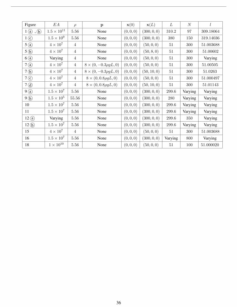
Figure EA ρ p x(0) x(L) L N l

1 a , b 1.5× 1011 5.56 None (0, 0, 0) (300, 0, 0) 310.2 97 309.18064

1 c 1.5× 109 5.56 None (0, 0, 0) (300, 0, 0) 380 150 319.14036

5 a 4× 107 4 None (0, 0, 0) (50, 0, 0) 51 300 51.003688

5 b 4× 107 4 None (0, 0, 0) (50, 8, 0) 51 300 51.00602

6 a Varying 4 None (0, 0, 0) (50, 0, 0) 51 300 Varying

7 a 4× 107 4 8× (0,−0.3ρgL, 0) (0, 0, 0) (50, 0, 0) 51 300 51.00505

7 b 4× 107 4 8× (0,−0.3ρgL, 0) (0, 0, 0) (50, 10, 0) 51 300 51.0263

7 c 4× 107 4 8× (0, 0.8ρgL, 0) (0, 0, 0) (50, 0, 0) 51 300 51.000497

7 d 4× 107 4 8× (0, 0.8ρgL, 0) (0, 0, 0) (50, 10, 0) 51 300 51.01143

9 a 1.5× 107 5.56 None (0, 0, 0) (300, 0, 0) 299.6 Varying Varying

9 b 1.5× 105 55.56 None (0, 0, 0) (300, 0, 0) 280 Varying Varying

10 1.5× 107 5.56 None (0, 0, 0) (300, 0, 0) 299.6 Varying Varying

11 1.5× 107 5.56 None (0, 0, 0) (300, 0, 0) 299.6 Varying Varying

12 a Varying 5.56 None (0, 0, 0) (300, 0, 0) 299.6 350 Varying

12 b 1.5× 107 5.56 None (0, 0, 0) (300, 0, 0) 299.6 Varying Varying

15 4× 107 4 None (0, 0, 0) (50, 0, 0) 51 300 51.003688

16 1.5× 107 5.56 None (0, 0, 0) (300, 0, 0) Varying 800 Varying

18 1× 1010 5.56 None (0, 0, 0) (50, 0, 0) 51 100 51.000020

36

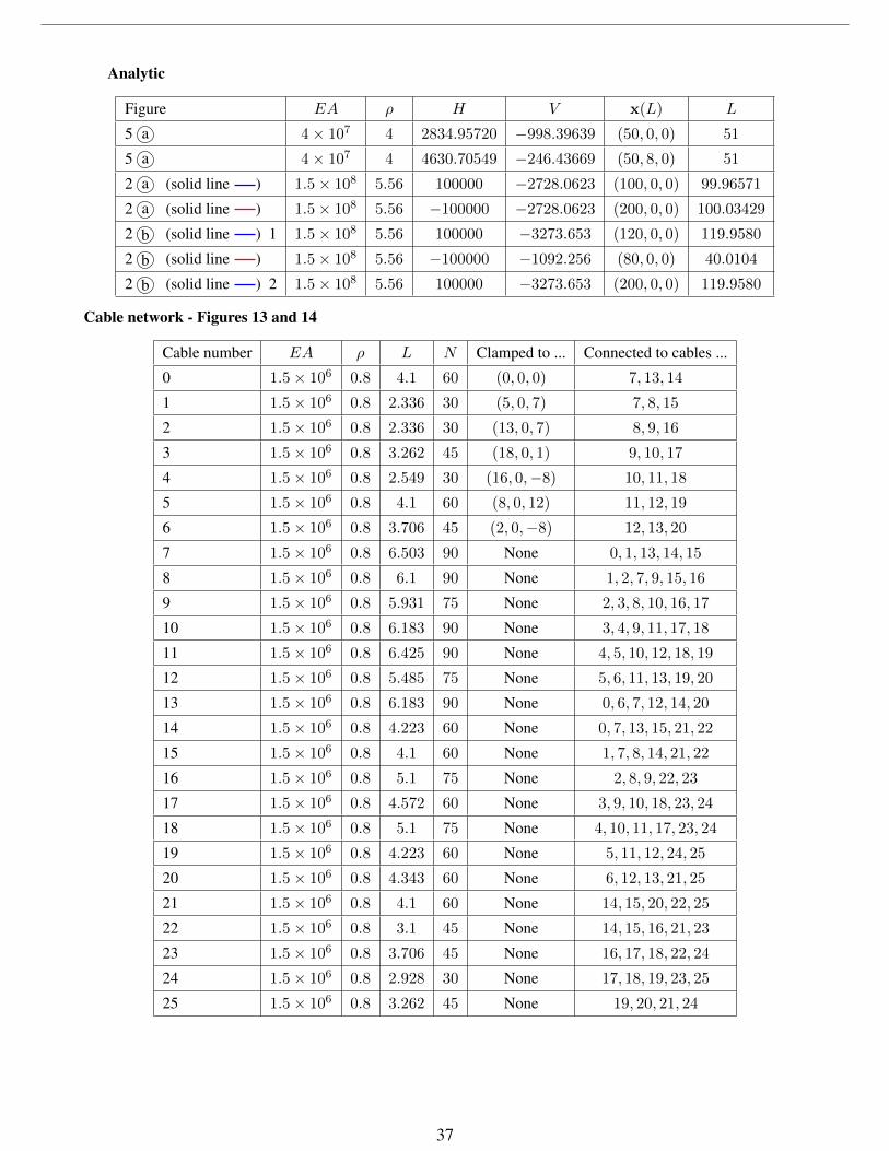
Analytic

Figure EA ρ H V x(L) L

5 a 4× 107 4 2834.95720 −998.39639 (50, 0, 0) 51

5 a 4× 107 4 4630.70549 −246.43669 (50, 8, 0) 51

2 a (solid line ) 1.5× 108 5.56 100000 −2728.0623 (100, 0, 0) 99.96571

2 a (solid line ) 1.5× 108 5.56 −100000 −2728.0623 (200, 0, 0) 100.03429

2 b (solid line ) 1 1.5× 108 5.56 100000 −3273.653 (120, 0, 0) 119.9580

2 b (solid line ) 1.5× 108 5.56 −100000 −1092.256 (80, 0, 0) 40.0104

2 b (solid line ) 2 1.5× 108 5.56 100000 −3273.653 (200, 0, 0) 119.9580

Cable network - Figures 13 and 14

Cable number EA ρ L N Clamped to ... Connected to cables ...

0 1.5× 106 0.8 4.1 60 (0, 0, 0) 7, 13, 14

1 1.5× 106 0.8 2.336 30 (5, 0, 7) 7, 8, 15

2 1.5× 106 0.8 2.336 30 (13, 0, 7) 8, 9, 16

3 1.5× 106 0.8 3.262 45 (18, 0, 1) 9, 10, 17

4 1.5× 106 0.8 2.549 30 (16, 0,−8) 10, 11, 18

5 1.5× 106 0.8 4.1 60 (8, 0, 12) 11, 12, 19

6 1.5× 106 0.8 3.706 45 (2, 0,−8) 12, 13, 20

7 1.5× 106 0.8 6.503 90 None 0, 1, 13, 14, 15

8 1.5× 106 0.8 6.1 90 None 1, 2, 7, 9, 15, 16

9 1.5× 106 0.8 5.931 75 None 2, 3, 8, 10, 16, 17

10 1.5× 106 0.8 6.183 90 None 3, 4, 9, 11, 17, 18

11 1.5× 106 0.8 6.425 90 None 4, 5, 10, 12, 18, 19

12 1.5× 106 0.8 5.485 75 None 5, 6, 11, 13, 19, 20

13 1.5× 106 0.8 6.183 90 None 0, 6, 7, 12, 14, 20

14 1.5× 106 0.8 4.223 60 None 0, 7, 13, 15, 21, 22

15 1.5× 106 0.8 4.1 60 None 1, 7, 8, 14, 21, 22

16 1.5× 106 0.8 5.1 75 None 2, 8, 9, 22, 23

17 1.5× 106 0.8 4.572 60 None 3, 9, 10, 18, 23, 24

18 1.5× 106 0.8 5.1 75 None 4, 10, 11, 17, 23, 24

19 1.5× 106 0.8 4.223 60 None 5, 11, 12, 24, 25

20 1.5× 106 0.8 4.343 60 None 6, 12, 13, 21, 25

21 1.5× 106 0.8 4.1 60 None 14, 15, 20, 22, 25

22 1.5× 106 0.8 3.1 45 None 14, 15, 16, 21, 23

23 1.5× 106 0.8 3.706 45 None 16, 17, 18, 22, 24

24 1.5× 106 0.8 2.928 30 None 17, 18, 19, 23, 25

25 1.5× 106 0.8 3.262 45 None 19, 20, 21, 24

37

REFERENCES

References

[1] E. Bobillier and M. Finck. Questions résolues. Annales de mathématiques pures et appliquées, Tome 17, pages

59–68, 1826.

[2] H. M. Irvine. Cable structures. Dover, New York, 1992. OCLC: 831328789.

[3] G. Rega. Nonlinear vibrations of suspended cables - Part I: Modeling and analysis. Applied Mechanics

Reviews, 57(6):443, 2004.

[4] N. Srinil, G. Rega, and S. Chucheepsakul. Three-dimensional non-linear coupling and dynamic tension in the

large-amplitude free vibrations of arbitrarily sagged cables. Journal of Sound and Vibration, 269(3-5):823–852,

2004.

[5] V. Gattulli, L. Martinelli, F. Perotti, and F. Vestroni. Nonlinear oscillations of cables under harmonic loading

using analytical and finite element models. Computer Methods in Applied Mechanics and Engineering,

193(1–2):69–85, 2004.

[6] J. Warminski, D. Zulli, G. Rega, and J. Latalski. Revisited modelling and multimodal nonlinear oscillations of

a sagged cable under support motion. Meccanica, 51(11):2541–2575, 2016.

[7] D. Bruno and A. Leonardi. Nonlinear structural models in cableway transport systems. Simulation Practice

and Theory, 7(3):207–218, 1999.

[8] Y. T. Tsui. Dynamic behavior of a pylône à chaînette line part I: Theoretical studies. Electric Power Systems

Research, 1:305 – 314, 1978.

[9] Y. T. Tsui. Dynamic behavior of a pylône à chaînette line part II: Experimental studies. Electric Power Systems

Research, 1:315 – 322, 1978.

[10] Y.M. Desai, P. Yu, N. Popplewell, and A.H. Shah. Finite element modelling of transmission line galloping.

Computers & structures, 57(3):407–420.

[11] Y. Kanno and M. Ohsaki. Minimum principle of complementary energy of cable networks by using second-

order cone programming. International Journal of Solids and Structures, 40(17):4437–4460, 2003.

[12] A.H. Peyrot and A.M. Goulois. Analysis of cable structures. Computers & Structures, 10(5):805–813, 1979.

[13] I. Fried. Large deformation static and dynamic finite element analysis of extensible cables. Computers &

Structures, 15(3):315–319, 1982.

[14] B.W. Kim, H.G. Sung, S.Y. Hong, and H.J. Jung. Finite Element Nonlinear Analysis for Catenary Structure

Considering Elastic Deformation. Computer Modeling in Engineering & Sciences, 63(1):29–46, 2010.

[15] M. Crusells-Girona, F. C. Filippou, and R. L. Taylor. A mixed formulation for nonlinear analysis of cable

structures. Computers & Structures, 186:50–61, 2017.

[16] J. J. Marigo. Mécanique des Milieux Continus I. Paris, École polytechnique, 2014. Lecture notes, HAL-ID:

cel-01023392.

[17] H. J. Ernst. Der e-modul von seilen unter berücksichtigung des durchhanges. Der Bauingenieur, 40(2):52–55,

1965.

[18] W. M. Henghold and J. J. Russell. Equilibrium and natural frequencies of cable structures (a nonlinear finite

element approach). Computers & Structures, 6(4-5):267–271, 1976.

38

REFERENCES

[19] O. C. Zienkiewicz and R. L. Taylor. The finite element method. Vol. 1: The basis. Butterworth-Heinemann,

Oxford, 5. ed., reprinted edition, 2002. OCLC: 249013082.

[20] C. A. Felippa. Finite element analysis of three-dimensional cable structures. Proc. 1st Int. Conf. Computational

Methods in Nonlinear Mechanics; Austin TX, pages 311–324, 1974.

[21] M. Tur, E. Garcia, L. Baeza, and F.J. Fuenmayor. A 3d absolute nodal coordinate finite element model to

compute the initial configuration of a railway catenary. Engineering Structures, 71:234–243, 2014.

[22] C. A. Felippa and B. Haugen. A unified formulation of small-strain corotational finite elements: I. Theory.

Computer Methods in Applied Mechanics and Engineering, 194(21-24):2285–2335, 2005.

[23] M. Rezaiee-Pajand, M. Mokhtari, and Amir R. Masoodi. A novel cable element for nonlinear thermo-elastic

analysis. Engineering Structures, 167:431–444, 2018.

[24] P. D. Panagiotopoulos. Stress-unilateral analysis of discretized cable and membrane structure in the presence

of large displacements. Ingenieur-Archiv, 44(5):291–300, 1975.

[25] M. Angelillo. A finite element approach to the study of no-tension structures. Finite Elements in Analysis and

Design, 17(1):57–73, 1994.

[26] M. A. Millar and Barghian M. Snap-through behaviour of cables in flexible structures. Computers & Structures,

77:361–369, 2000.

[27] V. Acary and B. Brogliato. Numerical methods for nonsmooth dynamical systems. Applications in mechanics

and electronics. Lecture Notes in Applied and Computational Mechanics 35. Berlin: Springer. xxi, 525 p. ,

2008.

[28] M. Abramovich and I. A. Stegun. Handbook of Mathematical Functions with Formulas, Graphs and Mathe-

matical Tables. Dover, New York.

[29] S. Ueber, G. Stadler, and B. Wohlmuth. A primal-dual active set algorithm for three-dimensional contact

problems with coulomb friction. SIAM J. Scientific Computing, 30.

[30] E.-D. Dolan and J.-J. Moré. Benchmarking optimization software with performance profiles. Mathematical

Programming, 91:201–213, 2002.

[31] G. Lallement and D. Inman. A Tutorial on Complex Eigenvalues. In Proceedings of 13th International Modal

Analysis Conference, volume 2460, pages 490–495, 1995.

[32] F. Brezzi, J. Rappaz, and P.A. Raviart. Finite dimensional approximation of nonlinear problem, part 1:

Branches of nonsingular solutions. Numerische Mathematik, pages 1 – 25.

[33] B. Fraejis de Veubeke, M. Gérardin, and A. Huck. Structural dynamics. LTAS, Liège, 1974.

39