A Revisionist Historyof

Algorithmic Game Theory

Moshe Y. Vardi

Rice University

Theoretical Computer Science:Vols. A and B

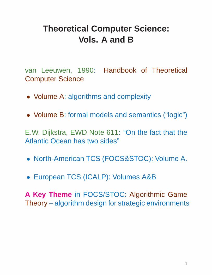
van Leeuwen, 1990: Handbook of TheoreticalComputer Science

• Volume A: algorithms and complexity

• Volume B: formal models and semantics (“logic”)

E.W. Dijkstra, EWD Note 611: “On the fact that theAtlantic Ocean has two sides”

• North-American TCS (FOCS&STOC): Volume A.

• European TCS (ICALP): Volumes A&B

A Key Theme in FOCS/STOC: Algorithmic GameTheory – algorithm design for strategic environments

1

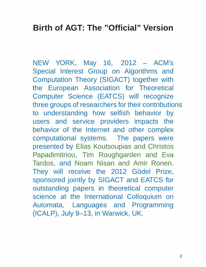
Birth of AGT: The ”Official” Version

NEW YORK, May 16, 2012 – ACM’sSpecial Interest Group on Algorithms andComputation Theory (SIGACT) together withthe European Association for TheoreticalComputer Science (EATCS) will recognizethree groups of researchers for their contributionsto understanding how selfish behavior byusers and service providers impacts thebehavior of the Internet and other complexcomputational systems. The papers werepresented by Elias Koutsoupias and ChristosPapadimitriou, Tim Roughgarden and EvaTardos, and Noam Nisan and Amir Ronen.They will receive the 2012 Godel Prize,sponsored jointly by SIGACT and EATCS foroutstanding papers in theoretical computerscience at the International Colloquium onAutomata, Languages and Programming(ICALP), July 9–13, in Warwick, UK.

2

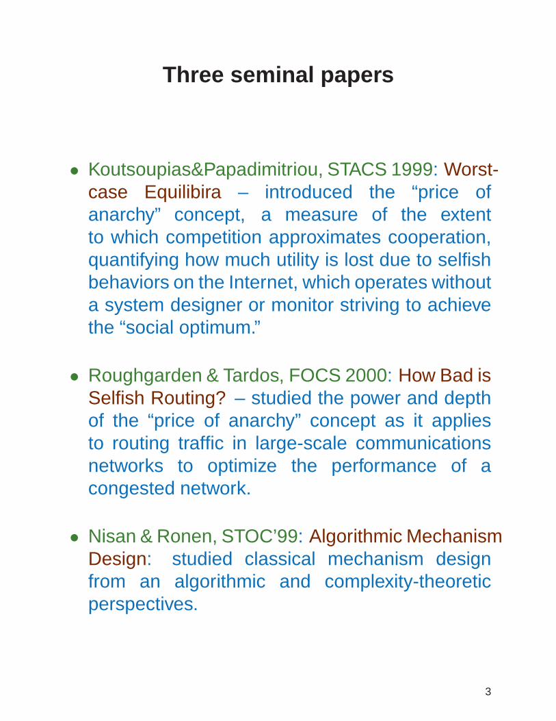
Three seminal papers

• Koutsoupias&Papadimitriou, STACS 1999: Worst-case Equilibira – introduced the “price ofanarchy” concept, a measure of the extentto which competition approximates cooperation,quantifying how much utility is lost due to selfishbehaviors on the Internet, which operates withouta system designer or monitor striving to achievethe “social optimum.”

• Roughgarden & Tardos, FOCS 2000: How Bad isSelfish Routing? – studied the power and depthof the “price of anarchy” concept as it appliesto routing traffic in large-scale communicationsnetworks to optimize the performance of acongested network.

• Nisan & Ronen, STOC’99: Algorithmic MechanismDesign: studied classical mechanism designfrom an algorithmic and complexity-theoreticperspectives.

3

Worst-Case Rquilibria – Price ofAnarchy

Question : What is the worst-case ratio betweencooperative (centralized) and non-cooperative (distributed)outcomes in games?

Koutsoupias&Papadimitriou – for a simple routinggame: n tasks over m links

• Upper Bound: O(√m logm)

• Lower Bound: Ω(logm/ log logm)

Roughgarden & Tardos – a more complex routinggame:

• Tight Bound: 43

4

Algorithmic Mechanism Design

Background – Game Theory

• Equilibria Analysis: analogous to algorithmanalysis

• Mechanism Design: analogous to algorithmdesign

– Design games with desirable equilibria – e.g.,second-price sealed-bid auction

Nisan & Ronen – n-distributed task-allocation game

• Upper Bound: n-approximation mechanism

• Lower Bound: No c-approximation mechanismfor c < 2.

5

Computing Equilibria

Daskalakis&Goldberg&Papadimitriou, STOC’06: Thecomplexity of computing a Nash equilibrium –

• Nash’s existence proof is nonconstructive (usingBrouwer’s Fixed-Point Theorem)

• Theorem : Finding a Nash equilibrium in three-players games is PPAD-complete.

• Result extended later to two-players games.

PPAD – polynomial-parity arguments on directedgraphs

• Generally believed not to be in PTIME for succintgraphs.

6

Algorithmic Game Theory, 2007

7

A Revisionist Thesis

Thesis :

• AGT was initiated by logicians in 1957!

• AGT was revitalized by Vol. B TCS in 1989!

• AGT has been active in Volume B TCS sincethen!

Point :

• First: Give credit where credit is due!

• More Significantly: Tear down the wall betweenVol. A and Vol. B!

8

Gale-Stewart Games

Gale-Stewart Game : an infinite-round, full-information, turn-based, two-player game

• Finite Action Set – A, Winning Set – W ⊆ Aω

• Players 0 and 1 alternate choosing actions in A –play is in Aω

• Player 0 wins if play is in W

Basic Concepts :

• Strategy: f : A∗ → A

• Determinacy: Either Player 0 or Player 1 has awinning strategy.

Question : When is a Gale-Stewart game determined?

• Determinacy holds easily for finite-round games(Zermelo).

Known Results

• Gale&Stewart, 1953: Determinacy for open andclosed winning sets

• Martin, 1975: Determinacy for Borel winning sets

• Beyond Borel: depends on set-theoretic axioms

9

Monadic Second-Order Logic

View an infinite word w = a0, a1, . . . over alphabet Aas a mathematical structure:

• Domain: 0, 1, 2, . . .

• Dyadic predicate: <

• Monadic predicates: Pa : a ∈ AMonadic Second-Order Logic (MSO) :

• Monadic atomic formulas: Pa(x) (a ∈ A)

• Dyadic atomic formulas: x < y

• Set quantifiers: ∃P,∀PExample : (∀y)((∃x)((y < x)) ∧ Pa(x)) – infinitelymany occurrences of a.

10

MSO Games

Church’s Problem, 1957 :

• Input: MSO formula ϕ

• W = models(ϕ) - game is determined!

• Analysis: Who wins the game?

• Synthesis: Construct a winning strategy forwinning player

Solution [Buchi&Landweber, 1969]:

• Analysis problem is decidable – nonelementary• Winning player has a finite-memory strategy.• Finite-memory strategy can be constructed

algorithmically.

Rabin, 1972: Simpler solution via tree automata.

Claim : This is the birth of AGT!

• An algorithmic approach to a game-theoreticalquestion.

• Algorithm design in a strategic setting.• Automated algorithm design!

But : Nonelementary lower bound [Stockmeyer,1974].

11

Finite-Memory Strategies

Transducers [EF Moore, 1956] – T = (Σ,∆, S, s0, ρ, δ)

• Σ - finite input alphabet

• ∆ - finite output alphabet

• S: finite state set

• s0 ∈ S: start state

• δ : S × Σ → S - transition function

• δ : S → ∆ - output function

Extending – ρ : Σ∗ → S, δ : Σ∗ → ∆.

• ρ(ǫ) = s0

• ρ(wa) = ρ(ρ(w), a)

• δ(w) = δ(ρ(w))

12

LTL Games: Rebirth of AGT

Complexity-Theoretic Motivation : Can we getaround the nonelementary bound?

Answer : Use LTL (Linear Temporal Logic) ratherthan MSO.

• No explicit quantifiers

• Temporal connectives: next, eventually, always,until, release

• Expressively equivalent to first-order logic; weakerthan MSO.

[Pnueli&Rosner, 1989]: Analysis and synthesis ofLTL games is 2EXPTIME-complete.

13

Linear Temporal Logic

Linear Temporal logic (LTL): logic of temporalsequences (Pnueli, 1977)

Main feature: time is implicit

• next ϕ: ϕ holds in the next state.

• eventually ϕ: ϕ holds eventually

• always ϕ: ϕ holds from now on

• ϕ until ψ: ϕ holds until ψ holds.

• π,w |= next ϕ if w • -•ϕ

- • -• -•. . .

• π,w |= ϕ until ψ if w •ϕ

-•ϕ

- •ϕ

-•ψ

-•. . .

14

Examples

Psalm 34:14: “Depart from evil and do good”

• always not (CS1 and CS2): mutual exclusion(safety)

• always (Request implies eventually Grant):liveness

• always (Request implies (Request until Grant)):liveness

15

What Good is Model Checking?

Model Checking :

• Given: Program P , Specification ϕ

• Task: Check that P |= ϕ

Success :

• Algorithmic methods: temporal specificationsand finite-state programs.

• Also: Certain classes of infinite-state programs

• Tools: SMV, SPIN, SLAM, etc.

• Impact on industrial design practices is increasing.

Problems :

• Designing P is hard and expensive.

• Redesigning P when P 6|= ϕ is hard andexpensive.

16

Automated Design of Programs

Basic Idea :

• Start from spec ϕ, design P such that P |= ϕ.

Advantage:

– No verification– No re-design

• Derive P from ϕ algorithmically.

Advantage:

– No design

In essence : Declarative programming taken tothe limit.

17

Program Synthesis

The Basic Idea : Mechanical translationof human-understandable task specificationsto a program that is known to meet thespecifications.

Deductive Approach [Green, 1969, Waldinger andLee, 1969, Manna and Waldinger, 1980]

• Prove realizability of function,e.g., (∀x)(∃y)(Pre(x) → Post(x, y))

• Extract program from realizability proof.

Classical vs. Temporal Synthesis :

• Classical: Synthesize transformational programs

• Temporal: Synthesize programs for ongoingcomputations (protocols, operating systems,controllers, etc.)

18

Synthesis of Ongoing Programs

Specs: Temporal logic formulas

Early 1980s : Satisfiability approach(Wolper, 1981, Clarke+Emerson, 1981)• Given: ϕ• Satisfiability: Construct M |= ϕ• Synthesis: Extract P from M .

Example : always (odd→ next ¬odd)∧always (¬odd→ next odd)

odd - odd

19

Reactive Systems

Reactivity : Ongoing interaction with environment(Harel+Pnueli, 1985), e.g., hardware, operatingsystems, communication protocols, etc.

Example : Printer specification –Ji - job i submitted, Pi - job i printed.

• Safety: two jobs are not printed togetheralways ¬(P1 ∧ P2)

• Liveness: every job is eventually printedalways

∧2j=1(Ji → eventually Pi)

20

Satisfiability and Synthesis

Specification Satisfiable? Yes!

Model M : A single state where J1, J2, P1, and P2

are all false.

Extract program from M? No!

Why? Because M handles only one inputsequence.

• J1, J2: input variables, controlled by environment

• P1, P2: output variables, controlled by system

Desired : a system that is receptive to all inputsequences.

Conclusion : Satisfiability is inadequate for synthesisof reactive systems.

21

Realizability

I: input variables, O: output variables

Game:

• System: choose from 2O, Env: choose from 2I

Infinite Play :i0, i1, i2, . . .00, 01, 02, . . .

Infinite Behavior : i0 ∪ o0, i1 ∪ o1, i2 ∪ o2, . . .

Win : behavior |= spec

Specifications : LTL formula on I ∪O

Realizability : [Abadi+Lamport+Wolper, 1989Dill, 1989, Pnueli+Rosner, 1989]Existence of winning strategy for system.

Synthesis [Pnueli+Rosner, 1989]:Extraction of winning strategy for system.

Question : LTL is subsumed by MSO, so whatdid Pnueli and Rosner do?Answer : better algorithms!

22

Post-1972 Developments

Pnueli, 1977 : Use LTL rather than MSO as speclanguage

V.+Wolper, 1983 : Exponential translation from LTLto Buchi automata

Safra, 1989 : Exponential determinization of Buchiautomata

Pnueli+Rosner, 1989 : 2EXPTIME realizabilityalgorithm wrt LTL spec

Rosner, 1990 : Realizability is 2EXPTIME-complete.

Post 1990 : Emergence of Parity Games

23

Distributed Games

[Pnueli&Rosner, 1990]: Can we synthesizedistributed protocols?

• Reduce to multi-player games

• Model communications via a directed graph

• Critical factor: complete vs. incomplete informatongames

Result : Complexity goes from 2EXPTIME tononelementary to undecidable.

• Finkbeiner&Schewe, 2005: characterization ofdecidability

Related Work : multiple-player games with incompleteinformation [Peterson&Reif, 1979]

24

Buchi Automata

Buchi Automaton : A = (Σ, S, S0, ρ, F )• Alphabet: Σ• States: S• Initial states: S0 ⊆ S• Transition function: ρ : S × Σ → 2S

• Accepting states: F ⊆ S

Input word : a0, a1, . . .

Run : s0, s1, . . .

• s0 ∈ S0

• si+1 ∈ ρ(si, ai) for i ≥ 0

Acceptance : F visited infinitely often

- •6

0

1-

0•

6

1

– infinitely many 1’s

Fact : Buchi automata define the class ω-Reg of ω-regular languages.

25

Logic vs. Automata

Paradigm : Compile high-level logical specificationsinto low-level finite-state language

Compilation Theorem : [Buchi, 1960] Givenan MSO formula ϕ, one can construct a Buchiautomaton Aϕ such that a trace σ satisfies ϕ ifand only if σ is accepted by Aϕ.

Complexity : nonelementary [Stockmeyer, 1974]

Exponential-Compilation Theorem [V. &Wolper,1983–1986]: Given an LTL formula ϕ ofsize n, one can construct a Buchi automatonAϕ of size 2O(n) such that a trace σ satisfies ϕif and only if σ is accepted by Aϕ.

Ongoing Research : practically effective compilation

26

Determinization

• Key Insight: Fundamental mismatch betweenautomaton nondeterminism and strategic behavior– determinization required!

• Obstacle: Buchi automata are not closed underdeterminization.

Deterministic Parity Automaton :A = (Σ, S, S0, ρ, F )• Alphabet: Σ• States: S• Initial states: S0 ⊆ S• Transition function: ρ : S × Σ → S• Accepting Condition: π :→ 0, . . . , k − 1 –priority function

Acceptance : minimal priority visited infinitely oftenis even.

Determinization Theorem [Safra,1988]: Given ann-state Buchi automaton A, we can construct anequivalent deterministic parity automaton Ad withnO(n) states and n priorities.

Ongoing Research : determinization constructions

27

Parity Games

Key Ideas in LTL Games : from logic to automata,from automata to graph games

Crux : Many synthesis and model-checking problemsare reducible to parity games.

Parity Games G = (V0, V1, E, π)

• V = V0 ∪ V1, E ⊆ V 2 – total relation

• Priorities: π : V → 0, . . . , k − 1• Play 0 moves pebble from V0, Play 1 movespebble from V0.

• Pebbles move along edges in E

• Play: Sequence in V ω

• Winning: Player i wins if minimum priority visitedinfinitely often has parity i.

Determinacy : game is determined!

• Analysis: Who wins from a given node v of aparity game G?

• Synthesis: construct winning strategy for winningplayer.

28

Parity Games – Known Result

Emerson&Jutla, 1991: Winner has a memoryless(i.e., history-free) strategy.

Parameters : n nodes, m edges, k priorities

Complexity :

• Jurdzinski, 1998: in UP∩co-UP

• Schewe, 2007: O(mnk3)

• Jurdzinski&Paterson&Zwick, 2008: randomizedalgorithm in O(n

√n)

• Friedmann&Hansen&Zwick, 2011: Subexponentiallower bound for a particular LP algorithm for PGs

Major Open Question : Are parity games solvablein PTIME?

29

Mean-Payoff Games

[Ehrenfeucht&Mycielski, 1979]: Mean-Payoff Games– G = (V0, V1, E, π)

• Payoff of a play: LimAvg of sum of priorities

• Player 0 maximizes, Player 1 minimizes

Optimization Problem : Compute the maximalvalue that Player 0 can guarantee at a given node.

Known :

• Jurdzinski, 1998: decision problem in UP∩co-UP

• Bjorklund&Sandberg&Vorobyov, 2003: randomizedsubexponential algorithm

A Bridge : Parity games are reducible to mean-payoff games, which are reducible to simplestochastic games [Jurdzinski, 1998, Zwick&Paterson,1996]

30

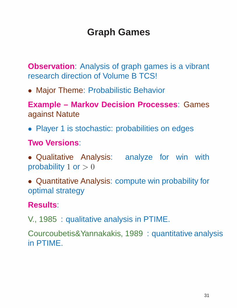
Graph Games

Observation : Analysis of graph games is a vibrantresearch direction of Volume B TCS!

• Major Theme: Probabilistic Behavior

Example – Markov Decision Processes : Gamesagainst Natute

• Player 1 is stochastic: probabilities on edges

Two Versions :

• Qualitative Analysis: analyze for win withprobability 1 or > 0

• Quantitative Analysis: compute win probability foroptimal strategy

Results :

V., 1985 : qualitative analysis in PTIME.

Courcoubetis&Yannakakis, 1989 : quantitative analysisin PTIME.

31

Incomplete Information

Incomplete Information : One or both players haveimperfect (but correct) sensors

Example : Parity Games with incomplete information

• Analysis and synthesis are EXPTIME-complete:follows from [Reif, 1984].

Combining Probability with Incomplete Information :Stochastic Games with Incomplete Information(following [Shapley, 1953])

Results for Stochastic Games :

• Complete Information: NP∩co-NP(Chatterjee&Jurdziski&Henzinger, 2004)

• One Player with Incomplete Information: undecidablequalitative analysis [Baier&Bertrand&Großer, 2008]

• One Player with Incomplete Information: undecidablequantitative analysis, even for finite-memorystrategies (follows from Paz, 1971); evenapproximate quantitative analysis is undecidable(Madani&Hanks&Condon, 2003)

• One Player with Incomplete Information: EXPTIME-complete qualitative analysis for finite-memorystrategies (Chatterjee&Doyen&Nain&V., 2014)

32

Synthesis from Components

Basic Intuition : [Lustig+V., 2009]

• In practice, systems are typically not builtfrom scratch; rather, they are constructed fromexisting components.– Hardware: IP cores, design libraries– Software: standard libraries, web APIs– Example: mapping application on smartphone

– location services, Google maps API,graphics library

• Can we automate “construction from components”?

Setup :

• Library L = C1, . . . , Ck of component types.• LTL specification: ϕ

Problem : Construct a finite system S that satisfiesϕ by composing components that are instances ofthe component types in L.

Question : What are components? How do youcompose them?

33

Components: Transducers with Exits

q0

0start

q1

1

q2

0

q3

1

a

b

b

a

b

a

34

Control-Flow Composition, I

Motivation : Software-module composition – exactlyone component interacts with environment at onetime; on reaching an exit state, goto start state ofanother component.

A library of two components types:L = M1,M2

35

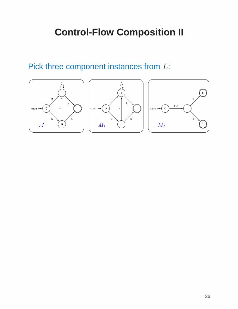
Control-Flow Composition II

Pick three component instances from L:

36

Control-Flow Composition III

Connect each exit to some start state – resultingcomposition is a transducer and is receptive.

37

Control-Flow Synthesis

Setup :

• Components: transducers with exit states, e.g.,software module

• Controlflow composition: upon arrival at an exitstate, goto start state of another component –composer chooses target of branch.

• No a priori bound on number of componentinstances!

Theorem : [Lustig+V.,2009]Controlflow synthesis from components is 2EXPTIME-complete.

Crux :

• Consider general (possible infinite) compositiontrees, that is, unfoldings of compositions

• Use tree automata to check that all possiblecomputations wrt composition satisfy ϕ

• Reduce to parity games• Show that if general composition exists then finite

composition exists.

38

Volume B AGT

Summary :

• Rich nearly-60-years-old theory

• Deep connections between logic, automata, andgames

• Fundamental motivation from SW/HW engineering

• Key: focus on algorithms and complexity

39

Mr. Gorbachev, Tear Down That Wall!

Vol. A and Vol. B AGT : Different but equal!

Vol. A → Vol. B :

• Complexity-theoretic approach to parity games– Parity Games Hypothesis (PGH): PG/∈PTIME‘– Consequences of PGH?

• Computing equilibria (e.g., “Rational Synthesis”,by Fisman&Kupferman&Lustig, 2010)

• Price of anarchy in quantitative synthesis,approximations, etc.

Vol. B → Vol. A :

• Extend from equilibria analysis to dynamicanalysis (e.g, “Network-Formation Games withRegular Objectives” by Avni&Kupferman&Tamir,2014).

• Automation of mechanism design (unpublishedby Chaudhuri&Fang&V.)

40