1

A Review on Computational Fluid Dynamics Modelling

in Human Thoracic Aorta

A.D. Caballero1 and S. Laín

1

1 Fluid Mechanics Research Group, Energetics and Mechanics Department, Universidad Autónoma de

Occidente, Cali, Colombia

Address correspondence to Santiago Laín, Energetics and Mechanics Department, Universidad Autónoma

de Occidente, Calle 25 No 115-85, Cali, Colombia. Electronic mail: slain@uao.edu.co

A.D. Caballero and S. Laín equally contribute to this article

Telephone: (57) 23188000 Ext. 11882

Email: slain@uao.edu.co

It has long been recognized that the forces and stresses produced by the blood flow on the walls of the

cardiovascular system are central to the development of different cardiovascular diseases. However, up to now,

the reason why arterial diseases occur at preferential sites is still not fully understood. This paper reviews the

progress, made largely within the last decade, towards the use of 3D computational fluid dynamics (CFD) models to

simulate the blood flow dynamics and its interaction with the arterial wall within the human thoracic aorta (TA).

We describe the technical aspects of model building, review methods to create anatomic and physiologic models,

obtain material properties, assign boundary conditions, solve the equations governing blood flow, and describe the

assumptions used in running the simulations. Detailed comparative information is provided in tabular format about

the model setup, simulation results, and a summary of the major insights and contributions of each TA article

reviewed. Several syntheses are given that summarize the research carried out by influential research groups,

review important findings, discuss the methods employed, limitations, and opportunities for further research. We

hope that this review will stimulate computational research that will contribute to the continued improvement of

cardiovascular health through a strong interaction and cooperation between engineers and clinicians.

Keywords: Blood flow, Computational fluid dynamics, Hemodynamics, Human thoracic aorta

2

1. Introduction

Aorta, the largest artery found in the human body, is the main vessel through which oxygenated

blood pumped out of the left ventricle (LV) enters the systemic circulation. Thoracic aorta (TA)

refers to the region that consists of the ascending aorta, aortic arch and descending aorta. This

segment also includes three main branches stemming from the arch, namely brachiocephalic artery

(BA), left common carotid artery (LCA) and left subclavian artery (LSA), which channel blood

supply to the upper parts of the body. TA has one of the most complex anatomies amongst all

arteries; in addition to bending severely, the centerline of the arch twists, thus it doesn’t lie in a

plane (non-planar). Additionally, TA has branching, tapering of the lumen and distensible arterial

walls.

Despite significant progress in clinical care and public education, cardiovascular diseases (CVDs)

remain the leading single cause of morbidity and mortality worldwide. According to a prediction

by World Health Organization, by year 2030 approximately 23.6 million people will die from

CVDs [47].TA with its complex anatomy is subjected to typical CVDs which often manifest in

forms of atherosclerosis, aneurysm, and dissection. Atherosclerosis, the most common

manifestation of arterial disease, is characterized by the thickening of the arterial wall caused by a

build-up of fatty plaque in the inner lining of the artery. Aortic aneurysm occurs when there is

progressive enlargement and dilation due to weakening of the aortic wall. Dissection, on the other

hand, refers to a disruption of the aortic wall, forming an intimal flap and therefore separating a

true from a false lumen. The above conditions are life-threatening due to their potential of rupture

at the weakened aortic sections, therefore, the need for elucidating the mechanisms involved in the

development and progression of these diseases is critical and has been the subject of active

research in the past decades.

Development of computational fluid dynamics (CFD) in recent years has enabled the use of 3D

numerical simulations to investigate patient-specific hemodynamics and to understand the origin

and development of different CVDs; mainly due to its capability of quantifying variables not

measurable in-vivo, its reproducibility, and its role as diagnostic and treatment tool for different

CVDs conditions. In contrast to in-vitro studies, CFD is more convenient for altering model

parameters such as boundary conditions, and given the complexity of blood flow in intricate

geometries, the combination between high resolution simulation techniques and image-based

measurements data has proven to be a reliable tool for realistic modelling of arterial blood flow.

Limitations in the use of CFD simulations are related primarily to the model assumptions that are

made when these simulations are performed, e.g. geometry, viscosity, distensibility, flow

conditions. Simplified interpretations, however, have always been the cornerstone of

understanding the physical world.

In spite of the last decade history of CFD studies related to the TA, this literature has never been

comprehensively reviewed. For new researchers entering the field, a critical review would be

invaluable, and experienced researchers who are focusing on a particular sub-problem may benefit

from an overview exposure to the work of other researchers. Thus, the goal of this paper is to

review the current state of the art of CFD modelling in human TA, including the main steps

involved in simulating blood flow and its interaction with the arterial wall, namely, problem

identification, pre-processing, solving, and post-processing. The article is organized as follows.

Section 2 begins by focusing on what is known about the biomechanical factors that play a role in

the cardiovascular health as well as in the progression and treatment of cardiovascular diseases.

Section 3 introduces the approaches of obtaining TA geometric models, discretization and meshing

schemes. Material properties, boundary conditions and turbulence models are also discussed.

Particular attention is paid to the assignment of boundary conditions, as this point is of critical

importance in the current area of research. Section 4 describes the governing equations and

important aspects of the mechanics of blood flow. Section 5 describes the post-processing,

including Table 1, which summarizes the major insights and contributions of each TA study

included in this review. Validation and verification of the computational results are also discussed.

Finally, Section 6 contains concluding remarks and future challenges.

3

2. Problem identification

The fact that mechanics plays a vital role in in the development and maintenance of cardiovascular

health, as well as in the initialization and localization of CVDs has been known since long;

however, it has only been since the mid-1970s that we have understood why mechanics are truly

important. Hemodynamic factors that have been suggested to influence cellular development on

the arterial wall are derived from the velocity field and involve several different forms, such as

flow separation, secondary flow, wall shear stress (WSS), and spatial and temporal shear stress

gradients. The relationship between shear stress distribution and cellular development has been

shown to be linked via the mechano-transduction process [48]. Particularly, endothelial cells

(ECs), which form the innermost layer of the arterial wall and are in direct contact with flowing

blood, can change their responses due to local flow conditions [49]. Several studies had shown that

endothelial dysfunction and arterial wall remodelling are correlated with complex flow dynamics;

especially with low and oscillatory shear stress [50-52]. The long term interaction between the ECs

and the blood flow results in changes of arterial wall thickness, structure and morphology,

processes directly linked to a variety of CVDs.

Today, there is accumulating evidence that atherosclerotic lesions occur predominantly at regions

of low and oscillatory shear [53-56]. Moreover, it is known that these lesions tend to localize in

regions of complex arterial geometry, such as bends, tapering, and branching [57-60]. Based on

these studies, the human TA with its complex anatomy can be considered as one of the most

susceptible arteries for the development of atherosclerosis. Bogren et al., Kilner et al. and Bogren

et al. [61-63] observed helical and retrograde (reversing) flow patterns prevailing in the aortic

arch. In these studies, the curvature and the non-planarity of the aortic arch were thought to be the

reasons for the helical nature of the blood flow. Later, Utepov et al. [64] demonstrated that the

tapering of the descending aorta is correlated with the progression of plaque in this part of the

aorta. Hence, besides hemodynamics factors, the global and local anatomy of an artery

significantly influences and plays a role in the initialization and localization of arterial diseases,

especially atherosclerosis.

Nevertheless, given the fact that early events leading to the pathogenesis of atherosclerosis is the

accumulation of lipids within the arterial wall, in recent years some researchers have been paying

more attention to mass transport phenomena in the cardiovascular system and the interaction of red

blood cells (RBCs) with the arterial wall [66-67]. An increased level of low-density lipoprotein

(LDL) has been shown to promote the accumulation of cholesterol within the intima layer of large

arteries [68-69]. There is an exchange of water from the blood to the arterial wall, driven by the

arterial pressure difference, which can transport LDL to the arterial wall. However, the ECs

present a barrier to LDL creating a flow-dependent concentration boundary layer. This

concentration polarization is interesting, as regions with elevated LDL are co-located with low

shear regions [70], suggesting a relationship between LDL accumulation and blood flow

dynamics. Studies in animals and humans have indicated that the flux of LDL from the blood into

the arterial wall depends both on the flow-dependent LDL concentration and the LDL permeability

at the blood–wall interface [71].

Oxygen transport in the arterial wall is probably another important factor involved in the

pathogenesis of atherosclerosis. Santilli et al. [72] observed that oxygen tension was significantly

lower at the atherosclerotic lesion-prone sinus region of the canine carotid sinus when compared

with that in the common carotid artery. In addition, hypoxia has been shown to cause damage to

the endothelial barrier and result in inter-endothelial gaps, hence leading to increased arterial wall

permeability to macromolecules [73]. Recently, Sluimer et al. [74] directly observed the existence

of hypoxia in human atherosclerotic carotid arteries for the first time. On the contrary, hyperoxia

has been shown to have the effect on the regression of atherosclerotic plaques [75]. Clearly, the

role of LDL and oxygen transport and its connection to atherosclerosis is a complex phenomenon,

present not only at two very different time scales but also at two very different spatial scales. To

this day, the reason why atherosclerosis development occurs at preferential sites is still not fully

understood, but these regions coincide with complex flow and low and oscillating shear stress.

These findings have motivated a large volume of research to try to elucidate the blood flow

dynamics in the human TA and to quantify the links between flow environment and CVDs

pathways.

4

3. Pre-processing

3.1 Geometry: definition of the computational domain

The first step on simulating blood flow is to obtain the geometry, or physical bounds of the artery.

There have been several experimental and computational studies in curved tubes, both in steady

and unsteady flow conditions, that have aimed to elucidate the flow dynamics in the aortic arch

[76-81]. These studies have provided great insight into the complexity of flow patterns in curved

tubes, established the influence of arch curvature, and documented the resulting skewness in

velocity profiles as well as the structure of secondary flow patterns within these geometries.

More recently, idealized geometries of the TA were also used in CFD studies (see Table 1).

Although the majority of these geometries were based on medical imaging data, some

simplifications were made, such as setting circular cross-sections, applying constant diameter

throughout the lumen or neglecting the arch branches. Mori & Yamaguchi [1] were amongst the

first researchers that used a magnetic resonance imaging (MRI) image-based geometry to simulate

blood flow in the TA. As a result, flow dynamics were more realistic in comparison to earlier

works with curved tubes. Later, Shacheraghi et al. [3] used a computed tomography (CT) image-

based geometry, and even though the TA model considered the arch branches and a minimal out-

of-plane curvature, it had a circular cross-section. While a major cause of complex flow dynamics

in large arteries is its local anatomy, the above idealized geometries captured important anatomical

features of the TA and were used to understand the extent of the idealization. Furthermore, these

studies in curved tubes and idealized geometries established the dependence of blood flow

dynamics on various geometric and model parameters, including the non-Newtonian behavior of

blood, fluid-structure interaction (FSI), mass transport phenomena, the flow Reynolds and Dean

numbers, and in the case of unsteady flow, the Womersley number.

While initially TA simulations were performed using idealized geometric models, in recent years

the majority of these studies have used image-based patient-specific geometries (see Table 1).

Currently, the most common medical imaging techniques used to reconstruct arterial geometries

are MRI and CT. On the one hand, CT is a technique used to obtain high resolution X-ray images

of the inside of a body with a very thin slice thickness. These images have high contrast which

makes it possible to see each part of a body distinctly by a slight adjustment of contrast. On the

other hand, MRI does not require the use of ionizing radiation; instead, contrast is achieved by

exploiting differences in the magnetic spin relaxation properties of the various bodily tissues and

fluids. For the purposes of imaging arteries, MRI is particularly attractive since the blood itself can

be used as a contrast agent. In addition, phase-contrast MRI (PC-MRI) may also be used to

measure time-varying blood flow rates waveforms to provide the necessary velocity boundary

conditions at the CFD model’s inlets and outlets

In general, after image acquisition, the 3D model reconstruction includes two major steps: image

segmentation and surface modelling. Many of the early tools for image-based reconstruction were

based on 2D segmentation [82, 83]. This approach is based on re-sampling the 3D image data on

2D image planes, segmenting the lumen boundary on this plane to obtain a closed-curve, lofting

adjacent curves to create a tubular model of the artery, and then using geometric union operations

to create the complete model. Although 2D segmentation can be used to create complex geometric

models and works particularly well for image data within regions of poor contrast, this approach is

largely manual and thus very time-consuming. More recently, a less time consuming, robust and

more automated alternative is 3D segmentation [84,85], as is used in commercial and open source

software packages. This approach uses intensity thresholding to automatically detect the imaging

area to be used in the model, thus it can present challenges with image data where contrast with

adjacent tissues is poor. These techniques can be performed with variants depending on the

software, with more or less automation as dictated by the resolution of the data.

3.2 Discretization: mesh generation

Once the anatomy has been translated into a 3D geometric model, it is discretized into a finite

number of smaller sub-domains called elements or cells, over which the governing Navier-Stokes

equations are then solved. The number and distribution of these elements largely govern the

accuracy of the simulation results; smaller elements must be used to resolve complex flow regions,

5

but the computational costs (time and memory) scale with the number of elements used, thus a

critical balance must be achieved between computational resources and solution accuracy.

In generating a spatial discretization of the computational domain, we are faced with the choice

between structured (hexahedral) or unstructured (tetrahedral) meshes. For curved tubes or

idealized TA geometries, structured meshing has been the preferred option, since is fairly

straightforward and can be easily automated by dividing the symmetric geometry into a fixed

number of points around the circumference and along the tube axis. Such structured meshes may

also be generated for the arch branches using block-structured meshes, though considerably more

effort is required to ensure the quality of the elements. In patient-specific TA simulations, the most

common approach has been the use of unstructured meshes produced by commercial meshing

software, in which distributions of tetrahedral, prismatic and pyramid elements are generated using

a variety of sophisticated algorithms. An unstructured computational domain is often preferred for

its potential of effortless grid generation over complex geometries, even though, structured meshes

may also be generated for patient-specific geometries.

A comparative CFD study between different mesh types in the TA is not yet available; however,

De Santis et al. [86] recently conducted a similar study in a left coronary artery. The results

showed that unstructured meshes needed much higher resolution than structured meshes to reach

mesh independency; with higher computational costs. Such differences are also reported in other

studies and are attributed to the poor alignment with the primary flow direction and to the high

numerical diffusion error associated with unstructured meshes [87]. Hexahedral meshes are known

to provide higher accuracy but are generally more difficult to generate in complex and branching

geometries, and the associated user intervention time can be excessively expensive. Figure 1

presents an example of MRI data at maximum intensity projection (a) used to derive a patient-

specific TA coarctation 3D geometric model (b) in combination with an unstructured mesh with

five prism layers adjacent to the arterial wall (c). Note that due to the nature of the imaging data,

the exact shape of the artery may differ from the one seen on MRI.

Mesh independence studies are a vital part of CFD work since they show the extent to which the

results depend on mesh parameters, and quantify the error associated with spatial discretization.

However, as noted by Prakash & Ethier [88], mesh refinement studies are rarely reported in the

literature. Where the results of a study are given, they are sometimes ambiguous, with simple

statements of the percentage error compared to a finer mesh. Without the densities of the two

meshes these statements give the reader no information about how well converged the solution is,

since by making a mesh which is only a little finer it is clearly possible to achieve a tiny

percentage difference between the two solutions [89]. Adaptive meshing techniques were recently

described for CFD studies. Muller et al. and Sahni et al. [90,91] discuss a method in which a-

posteriori error estimators, provide necessary information to adaptively refine the mesh.

Furthermore, because the resolution of WSS is often of interest, boundary layer mesh generation

techniques can be used to increase mesh density near the arterial wall [92]. In retrospect, a valid

computational mesh should accurately resolve both the complex geometry and the physiologically

relevant flow features, and should take the user, the solver and the computational resources out of

the loop.

3.3 Material properties

3.3.1 Human blood

Human blood which exhibits a highly complex, flow-dependent physical and chemical

constitution, is a non-Newtonian fluid in which its viscosity depends on the shear rate. Blood

viscosity is shear-thinning because of the disaggregation of the rouleaux (stacks of RBCs) and the

orienting of individual RBCs [93]. Experimental evidence has also shown that blood under certain

conditions behaves as a non-linear viscoelastic fluid, resulting from the elastic membranes of its

constituents [94]. Finally, blood is thixotropic; its viscosity can vary with time at constant low

shear mainly due to rouleaux aggregation and disaggregation. Although blood has been usually

considered as a Newtonian fluid in CFD studies of large arteries, its viscosity is strongly

influenced by two factors: hematocrit (volume percentage of RBCs in whole blood) and

temperature. As hematocrit increases, there is an increase in viscosity, as temperature decreases,

viscosity increases [95].

6

It can be seen that most of the rheological models proposed in the literature to predict the stress

versus strain rate relationship of blood fall into two categories: (i) models which predict shear-

thinning effects: the Cross model [96], the non-Newtonian Power law model [97], the Carreau

model [98] and the Second-grade model [99], (ii) models which exhibit yield stress: the Casson

model [100] and the Herschel–Bulkley model [101]. Moreover, complex constitutive models in

which blood is modeled as a viscoelastic fluid have also been introduced [102]. Although

constitutive equations from the Oldroyd-B type model have the best potential to capture with

reasonable accuracy the rheological behavior of blood in large arteries [103], the remaining

challenge is to determine and develop more sophisticated non-Newtonian models that capture

blood real behavior under complex flow conditions.

Experimental studies have shown that at high shear rates (above 100 s−1

) and in large and medium

arteries, the viscosity of human blood with 45 % hematocrit reaches a constant value of 3.0 - 4.0

mPa s [104], thus justifying somewhat the choice of a Newtonian model. However, there does not

appear to be a consensus in the literature on the importance of the non-Newtonian effects of blood

in large arteries, including the TA. While some studies have found significant differences between

their results calculated with and without the non-Newtonian models [105-107], others have found

that the Newtonian approach is a reasonably good approximation [108,109]. The main argument to

ignore the non-Newtonian behavior of blood is that shear rates in large arteries are predominantly

high. Still, in transient flow conditions, especially when the blood flow slow or reverses direction,

there are periods of time and local regions where the shear rate may be below 100 s-1

and it would

be reasonable to expect that the non-Newtonian effects may be important. The question that is

important to address is; to what extent are these effects important over an entire cardiac cycle?

A recent study by Liu et al. [25] investigated the effect of both non-Newtonian and pulsatile blood

flow conditions on mass transport phenomena in a patient-specific TA model. It was found that

under steady flow conditions, although the WSS distribution is similar for both the Newtonian and

the non-Newtonian simulations, the WSS magnitude for the non-Newtonian simulation is

generally higher than that for the Newtonian simulation, especially in areas with low WSS. The

steady results also revealed that when compared to the Newtonian simulation, the shear thinning

non-Newtonian behavior of blood (Carreau model) has little effect on LDL and oxygen transport

in most regions of the TA, but in atherogenic-prone areas (areas with flow disturbance) where the

luminal surface LDL concentration is high and oxygen flux is low, its effect its apparent. The

effect of flow pulsation on the transport of LDL has a similar trend. But pulsatile flow can

apparently enhance oxygen flux in the TA, especially in areas predisposed to flow disturbance

(low oxygen flux). Therefore, it was suggested that the shear thinning non-Newtonian behavior of

blood may be pro-atherogenic, while the pulsation of blood flow may be anti-atherogenic.

3.3.2 Arterial wall - FSI

The arterial wall deforms under loads, and in particular for some arteries such as the TA, this

deformation is large and might not be approximated by a rigid wall. In fact, the motion of the

arterial wall and surrounding tissues affects the blood flow dynamics and vice versa, both in

healthy and diseased conditions. Furthermore, wave propagation phenomena in the cardiovascular

system can only be modelled by taking the vessel wall deformability into account. Devising an

accurate model for the mechanical behavior of the arterial wall is a challenging task, since the

vessel wall is anisotropic, heterogeneous, and composed of three layers (intima, media and

adventitia) with different biomechanical characteristics [110]. An accurate model for the arterial

wall should take into account the effects of anisotropy due to the distribution of the collagen fibers,

the three-layer structure, the nonlinear behavior due to collagen activation, the incompressibility

constraint, the surrounding tissues and the spatial variations in the vessel wall properties.

Modelling the interaction between the blood flow and the arterial wall represents one of the major

challenges in the field of CFD hemodynamics. Prior to 2005, with the exception of the work

developed by [4,5,111-113], and due mainly to the difficulties in formulating and solving the

coupled problem of fluid and solid, nearly all blood flow simulations were conducted in rigid-wall

models. However, in recent years, significant progress has been made in the area of FSI.

Traditional FSI techniques can be divided into four categories on the basis of the utilized

computational framework: linearized kinematics [114,115], coupled momentum method (CMM)

[116], immersed boundary method [117,118], and the arbitrarily Lagrangian-Eulerian (ALE)

formulation [119,120].

7

Several authors have successfully simulated blood flow in TA models using ALE methods and

non-ALE methods (see Table 1). To the best of our knowledge, the first full FSI simulation of

blood flow in the TA was performed by Gao et al. [8] on an idealized three-layer structure. The

FSI system was formulated in an ALE frame and solved under unsteady flow conditions. Despite

the predictions of blood flow dynamics utilizing an FSI technique, there were limitations to the

present study. Among these were neglecting the arch branches, the aortic arch's non-planarity and

the approximation of wall thickness. In general, ALE formulations are computationally expensive

when considering large models of the vasculature, and less robust than linearized kinematics

methods, since the mesh is deformed dynamically to always conform to the boundaries of the

computational domain, requiring the continual update of the geometry of the fluid and the

structural elements.

Later, Kim et al. [18] presented a comprehensive FSI simulation in a patient-specific healthy TA

model under rest and exercise conditions and a in a TA coarctation model under pre and post-

intervention. The study used the CMM to describe the deformable wall properties and a coupled

lumped parameter (zero-dimensional) heart model as an inlet boundary condition. The structure

was mechanically constrained with fixed supports at the inlet and uniform deformable wall

properties were considered, despite the fact that the arterial wall properties vary spatially.

Although previous studies [121,122] have used lumped parameter heart models, these studies were

developed with the assumption of rigid arterial walls. In particular, the CMM shows good results

in many physiological situations and it has the advantage of being computationally inexpensive

because the mesh is fixed. Although the CMM is well suited for small displacements, this

approach can be inappropriate when the displacements become large. Furthermore, as the fixed

control volume where the fluid equations are solved allows the fluid to pass through the interface,

the quantities computed at the boundary, such as the WSS, are subject to a further approximation.

Most recently, Brown et al. [39] reported an alternative middle-ground approach to a full FSI

simulation. It employed a compressible fluid model tuned to elicit a response analogous to the

compliance of the TA wall, and thus to capture the wave propagation characteristics. It was

stressed that changes in fluid density represent the capacity for changes of fluid mass within a

cross-section, analogous to vessel wall compliance. The results showed that the use of a

compressible fluid model, set to produce the desired wave speed, was able to capture the gross

effects of the propagating waves. Furthermore, the results were significantly closer to those

obtained from a full FSI simulation than those produced by a rigid wall model, but at relatively

low computational costs. Although the compressible flow analysis over-estimates the WSS during

systole, it does capture the relative distribution of WSS and may offer a computationally viable

alternative to a full FSI model.

Without question, FSI in the arterial system depend strongly on the tissue and organs outside the

vessel of interest. Thus, a critical prerequisite for simulating realistic TA hemodynamics is the

development of patient-specific constitutive models for the cardiac tissue that account for the

complex interaction of the blood flow with the compliant and continuously deforming heart walls.

The development of patient-specific FSI simulations is a formidable task since total heart function

emerges as the result of the coupled interaction of the blood flow with a molecular, electrical and

mechanical processes that occur across a wide range of scales [123]. The first attempt to develop

3D models with coupled FSI simulation of blood flow and tissue mechanics was the pioneering

work by Peskin [124,125]. In this model the heart was assumed to be embedded in a periodic

domain filled with fluid and the simulations were carried out under conditions that were not

physiologic. More recently, different versions of this model have been able to carry out

simulations at higher cardiac volume flow rate [126-127], and other models have attempted to

raise the degree of patient- specific modelling realism by incorporating information acquired from

non-invasive imaging techniques [128-129]. The main challenges confronting this class of models

stem from the limitations in the resolution of imaging modalities, as well as the extensive

simplifying assumptions that need to be incorporated in the FSI model. To yield clinically relevant

results, these models need to be drastically enhanced by incorporating into the modelling

framework multi-physics elements of cardiac function along with inputs from modern imaging

technologies and in-vivo measurement techniques. Modelling the entire heart system would

necessitate a modelling effort as complex as for the problem at hand, i.e. FSI in the TA.

8

In conclusion, compared to a rigid wall model, FSI can provide a more accurate and physiologic

description of the hemodynamics as well as the arterial wall stresses and strains. Nevertheless, this

comes at the cost of requiring more complex numerical algorithms, higher computational costs,

and determination of patient-specific arterial wall properties, which are difficult to obtain

experimentally or are often unknown. As noted by Taylor & Figueroa [130], new imaging

techniques enable the characterization of the motion and thickness of the arterial wall; however, it

remains a challenge to incorporate this in-vivo data into FSI formulations. A new class of image-

based FSI problems will require the development of non-invasive methods to assign tissue

properties to the computational model from the medical imaging data, via the solution of an

inverse problem. Any CFD model that is intended for clinical application should capture the

important physical characteristics, but should be no more complex than it needs to be. Whether or

not FSI is included, the equations can only be solved if appropriate boundary conditions are given.

3.4 Boundary conditions

The cardiovascular system is a closed network with millions of vessels interacting with each other.

Since the input parameters to the CFD simulation are the boundary conditions, its choice plays a

major role in modelling the upstream and downstream vasculatures absent in the computational

domain of interest and must be carefully tuned to match clinical data. The question of where to cut

this domain is not trivial: the further the boundary is from the area of interest, the less influence

this artificial boundary will have on the local results, but the larger the computational domain will

be. Inappropriate boundary conditions would result in non-physical solutions.

3.4.1 Inlet boundary conditions

Usually, at the upstream side of the artery of interest a velocity boundary condition is prescribed at

the inlet, with an idealized profile such as a flat (plug), fully developed (parabolic) or Womersley

flow pattern, or based on time-varying velocity data obtained with PC-MRI or ultrasound (see

Table 1). Particularly, a flat velocity profile used together with a pulsatile waveform is often the

preferred inlet boundary condition in transient TA studies. This pulsatile waveform is generally

based on experimental data reported by Pedley [104], and it is characterized by accelerating,

decelerating, reversed, and zero flow regions (Figure 2). The assumption of a flat velocity profile

at the aortic inlet has been verified by various in-vivo measurements using hot-film anemometry

on different animal models, which have demonstrated that the velocity profile distal to the aortic

valve is essentially flat in the ascending aorta, skewed towards the inner wall with respect to the

aortic arch and only consisted of a weak helical component [131-133].

However, the fact is that the blood flowing into the TA pumped by the LV exhibits a complex 3D

nature. Blood flow patterns in the healthy TA range from axial during the early portion of systole,

to helical during mid-to-late systole, and complex flow recirculation during end systole and

diastole (Figure 3) [62]. The development of helical flow patterns during peak to late systole is

thought to be produced by several factors: (i) due to the arrangement of the muscle fibers, the LV

undergoes a significant torsional deformation, twisting in a counterclockwise direction during

systole and then returning in a clockwise direction during diastole, resulting in diastolic recoil; (ii)

the opening and closing dynamics of the aortic valve leaflets and their asymmetric configuration;

and (iii) the curvature and the non-planarity of the TA. As aortic helical flow is a common feature

in normal individuals as the consequence of the natural optimization of fluid transport processes in

the cardiovascular system [62,134], and it is strictly related to transport phenomena of oxygen and

LDL [19,22,25,37], great attention should be put when idealized velocity profiles are applied at the

inlet boundaries of TA computational models.

On the other hand, time-varying pressure waveforms, usually available from catheterization based

pressure acquisition technologies, are less frequently prescribed as inlet boundary conditions

[12,40]. Although it is claimed that the driving force for the blood flow in an artery is the pulsatile

pressure gradient along the artery, the amount of blood flowing in the computational model is very

sensitive to pressure gradients between inlet and outlets. As the pressure differences between these

boundaries are only a small percentage of the systolic-diastolic pulse amplitude, this imposes the

problem of accurately determine the pressure, a condition that is difficult to reach in practice.

Thus, small errors in the imposed pressure data could lead to great departure of the velocities from

the actual values. Moreover, patient-specific pressure data is not currently acquired with enough

precision to serve this purpose since an invasive approach could introduce sources of error and

9

artefacts such as deterioration in frequency response, catheter whip artefact, end-pressure artefact,

and systolic pressure amplification in the periphery, among others [135].

In contrast to several developments made in the area of outlet boundary conditions, little progress

has been reported for the influence of inlet boundary conditions in CFD studies of large arteries,

despite the fact that proximal to the inlet boundary there is also an upstream part of the

cardiovascular system that interacts with the computational domain. Additionally, and with the

exception of [17,46], no studies have investigated the effect of different inlet velocity profiles in

the TA, and few have reported its effect in other large arteries [136-139]. Morbiducci et al. [46]

studied how flat and fully developed inlet velocity profiles affect patient-specific simulated

hemodynamics in the TA when compared to simulations employing PC-MRI measured 3D and

axial (1D) velocity profiles of the patient’s own in-vivo measured flow data. The obtained results

were compared in terms of WSS distribution and helical flow structures. It was found that the

imposition of PC-MRI measured axial velocity profiles at the inlet may capture disturbed shear

with sufficient accuracy, without the need to prescribe (and measure) realistic fully 3D velocity

profiles. Likewise, attention should be put in setting idealized or PC-MRI measured axial velocity

profiles at the inlet of the TA computational model when transport phenomena are investigated,

since helical flow structures are markedly affected by the boundary condition prescribed at the

inlet.

While the above TA studies used inlet boundary conditions only valid for one particular

physiologic state, thus, ignoring the bidirectional interactions between the computational domain

and the heart, other TA studies have implemented reduced-order heart models as inlet boundary

conditions (see Table 1). Particularly, Kim et al. [18] developed and implemented a boundary

condition that coupled a zero-dimensional (lumped parameter) heart model to the inlet of a patient-

specific TA model, where the shape of the velocity profile of the inlet boundary were constrained.

It was stated that in order to study how the changes in the cardiac properties and the cardiovascular

system influence each other, the inlet boundary condition should model the interactions between

them. While the aortic valve is open, the aortic flow and pressure, and the ventricular pressure and

volume are computed through the coupling between the heart model and the TA model. When the

aortic valve closes, the inlet boundary condition switches to a zero velocity boundary condition.

Lumped parameter heart models approximate global characteristics of the heart using simple

hydraulic models of resistance, capacitance, inductance parameters, pressure source and diode,

resulting in time varying ordinary differential equations of flow and pressure.

3.4.2 Outlet boundary conditions

For the downstream side of the artery of interest, the boundary conditions have been a topic of

debate and continuous development in the last years. In physiological conditions, arteries are

branched and connected to smaller vessels, it is impossible to trace all the branching in the

simulation and the model must be terminated at some point, depending on the specific aim of the

study. Furthermore, these branches have to be lumped into a suitable terminal description, so that

wave propagation and artery impedance characteristics can be reasonably represented.

Previously, the most common outlet boundary conditions for CFD simulations of large arteries

were prescribed constant or time-varying pressures, constant (generally zero) traction and velocity

profiles (see Table 1). Such boundary conditions are limiting in that they do not accurately

replicated the fluid impedance of the downstream vasculatures. Particularly, if zero or equal

pressures or tractions are used for different outlets, the flow split will be dictated solely by the

resistance to flow in the branches of the domain of interest, neglecting the dominant effect of the

resistance of the downstream vasculatures [140,141]. Additionally, with constant pressure, zero

traction, and velocity as outlet boundary conditions, computed blood pressure is not in the

physiologic range and simulations could not be performed where the flow distribution and

pressure field are part of the desired solution [142,143].

In the case of time-varying velocity or pressure boundary conditions, first, obtaining such data for

a model with multiple outlets is impractical. Second, even if this data was acquired simultaneously

for each outlet, it would be very difficult to synchronize these waveforms in a manner consistent

with the wave propagation phenomena in the arterial wall. Yet, with electrocardiogram gated

measurements, there is likely to be a mismatch between the real and simulated wave speeds, which

may results in spurious reflections within the computational domain. Finally, prescribing time-

10

varying data is not relevant for treatment planning applications, where the quantity of blood flow

exiting and the distribution of pressure are unknown and are part of the desired solution.

Nevertheless, Gallo et al. [36] recently investigated how the imposition of personalized PC-MRI

measured blood flow rates as outlet boundary conditions influences the simulation results in a TA

model. From six different outlet strategies to manage the acquired flow data, it was concluded that

in order to obtain physiologically realistic results, the measured flow rates needed to be imposed at

three of the four outlets of the TA model.

Another approach widely described in the literature is to prescribe outflow boundary conditions at

the outlets as constant fractions of the inflowing blood (see Table 1). According to Middleman

[144], approximately five percent of the blood flow is assumed to leave the TA through each of the

three arch branches, though some CFD studies have recalculate these percentages based on the

specific outlet area of each arch branch or have used a modified version of the Murray's Law

[145]. However, this flow ratio is not a realistic approximation for patient-specific FSI models, and

there is no reason to believe that the flow division through the arch branches is constant during the

entire cardiac cycle [146].

To overcome the shortcomings of the above boundary conditions, other studies have used

simplified boundary conditions that include either resistance or impedance models [147,148]. In

the TA study developed by Park et al. [12], organs and body parts were assumed to be likened to

cylindrically shaped porous media, so-called “pseudo-organs”, and treated in the computational

domain as forms of hemodynamic resistance. Permeability functions were determined from two-

dimensional axisymmetric computations of each aortic branch. It was stated that there is a close

similarity between blood flow through small vessels and the fluid flow through a porous medium.

Thus, a proper permeability function could mimic flow through organs and body parts. Although

resistance boundary condition do not require the specification of either flow rate or pressure data,

it severely impacts wave propagation phenomena, since it forces the blood flow and pressure

waves to be in phase at the outlet and it can generate abnormal pressure values in situations of

flow reversal [149].

Increasingly, more sophisticated zero-dimensional (lumped parameter) models and 1D (distributed

parameter) models have been used in multiscale (or multidimensional) models, in which their

primary role is to provide boundary conditions for 3D computational simulations. For the 1D

network models, branching patterns, length, diameter, and material properties of vessel segments

are assigned; whereas for the lumped-parameter models, resistance, capacitance and inductance

parameters are set to achieve the desired hemodynamic characteristics of the downstream domain.

The coupling between these models can be solved in an explicit, staggered manner, or by

embedding the reduced-order model into the equations of the 3D computational domain. A lumped

parameter model is a dynamic description of the physics neglecting the spatial variation of its

parameters and variables. If the model is distributed, these parameters and variables are assumed

to be constant in each spatial compartment. Therefore, a lumped parameter model is governed by a

group of ordinary differential equations that assume a uniform distribution of the fundamental

variables (pressure, blood flow and volume) within any particular compartment of the

cardiovascular system at any instant in time, whereas a distributed parameter model can be

described by hyperbolic partial differential equations that recognise the variation of these

parameters in space. This is illustrated in Figure 4. A comprehensible review of zero-dimensional

and 1D models of blood flow in the cardiovascular system can be found in [150].

Several studies have successfully coupled distributed parameter models to 3D models [151-154],

including some TA studies (see Table 1). However, solving the transient nonlinear 1D equations of

blood flow in the millions of downstream vessels is an intractable problem, and therefore

linearized 1D models are needed. These simplified linear methods usually assume periodicity of

the solution [149,155,156]. Yet, blood flow and pressure in large arteries are not always periodic

in time due to heart rate variability, respiration, physiological changes or complex transitional flow

[157]. On the other hand, some studies have successfully coupled lumped parameter models to 3D

models [158-161], including some TA studies (see Table 1). Different strategies for coupling the

3D equations with lumped parameter models have been presented in [162,163]. However, in the

majority of these studies the coupling has been performed iteratively, which can lead to stability

and convergence issues, and has been generally applied to geometries with one or two outlets,

rigid walls and low resistances (as seen in the pulmonary vasculature). In contrast, a recent work

presented by Vignon-Clementel et al. [164] extended the multiscale modelling to include boundary

11

conditions that accommodate the non-periodic or transient phenomena using lumped parameter

outlet boundary conditions. This approach considered the arterial wall response to blood flow and

pressure on patient-specific multi-branched geometries.

Although with multiscale models, outlet boundary conditions are derived naturally through the

coupling of the 3D computational domain and the downstream reduced-order models, the

relationship between flow and pressure at each interface is generally enforced weakly, as a result

of the coupling between a numerical domain and analytic domain; which usually results in

diverging simulations. This coupling usually does not include any constraints on the shape of

velocity profiles nor on the pressure distribution at the interface. Yet, reduced-order models are

derived based on an assumed shape of the velocity profile and the assumption of uniform pressure

over the cross section [166,166]. As a result, some remaining challenges persist; these include

problems where flow is complex, with significant flow reversal during part of the cardiac cycle,

and with complex flow structures developing at the outlet boundaries due to vessel curvature or

branches immediately upstream of the boundary.

A common but rather rudimentary workaround to this problem has consisted of extending the

outlet branches using long straight segments to regularize the blood flow. Recently, new

formulations have been developed to resolve this issue numerically. Formaggia et al. [167]

implemented a total pressure boundary condition to control the energy flux entering and exiting

the computational domain and to stabilize problems with complex flows near boundaries.

However, this approach requires an unconventional formulation of the Navier-Stokes equations

and has not yet been proven to resolve boundary instability issues in complex hemodynamic

simulations. An alternate solution to this problem has been proposed by Kim et al. [18], where an

Augmented Lagrangian formulation was used to constrain the shape (but not the magnitude) of the

velocity profile at the inlet or outlet boundaries, rendering stable solutions regardless of the

complexity of the blood flow.

3.4.3 Arterial wall boundary conditions

Whereas much work has already been accomplished concerning outlet boundary conditions, few

CFD studies have taken into account the external tissues surrounding the TA to derive adequate

boundary conditions for the arterial wall domain (see Table 1). Large arteries subject to a high

load, as it is the case in the TA, undergoes large deformations concerning both the luminal radius

and the vessel displacement displacements, and experiences a complex coupling with surrounding

tissues and organs, namely interactions with the spine on the outer wall and with the heart in the

ascending aorta. However, in the majority of the FSI studies we are aware of, a free stress

condition with a constant (frequently zero) pressure has been applied on the outer part of the

arterial wall. This simple boundary condition is not able to sustain the artery and typically results

in non-physiological motion patterns of the arterial wall. In fact, this motion induces inaccuracies

much greater than those introduced by spurious reflections caused by inconsistent inlet and outlet

boundary conditions.

To take into account the influence of the heterogeneous tissue surrounding the TA, Crosetto et al.

[26] introduced a Robin condition [168] at the outer arterial wall. This condition consisted of a

pressure-displacement linear constitutive relation; relation previously investigated in-vivo and in-

vitro by Liu et al. [161]. In the latter work, the intraluminal pressure was shown to be proportional

to the radius of the lumen only when the surrounding tissue was taken into account. The main

difficulty encountered by Crosetto et al. [26] was to configure a suitable choice of one of the

models parameter. Though this choice was empirical, the results led to physiological

displacements and fitted qualitatively with the plot reported by Liu et al. [169]. It was found that

the pulse wave velocity, WSS, mean pressure, velocity and intraluminal radius at different axial

sections along the artery were in the physiological range, though many parameters have to be

adapted on a patient-specific basis. To the authors´ knowledge, this was the first FSI study that

addresses the formulation of an adequate boundary condition for the external tissue when studying

the TA.

Similarly, Moireau et al. [41] introduced a boundary condition along the TA outer wall that

consisted of a viscoelastic term representing the support provided by the surrounding tissues and

organs. A forcing term was used at the inlet boundary of the arterial wall to account for the heart

motion. This simple model corresponds to a generalized Robin condition on the walls and relies on

12

two adjustable parameters to mimic the response of various physiological tissues. Time-varying

medical imaging data was used to obtained information on the apparent motion of the wall. In

order to illustrate the versatility of this approach, two different patient-specific modelling cases

were implemented, using a distinct FSI technique for each (ALE and CMM). When applied to an

inlet or outlet arterial wall boundary, the viscoelastic term represents the truncated arterial tree

extending from the geometric model. Comparably, when applied along the exterior surface of the

arterial wall, the viscoelastic term models tethering to the external organs. This approach was

shown to improve the quality of the simulations by providing accurate deformation patterns of the

arterial tree. However, this required a careful manually calibration process of the parameters in the

boundary support model. More recently, Moireau et al. [170] proposed a method to automate and

refine this calibration process. A complete methodological chain for the identification of boundary

support parameters in a TA model based on well-adapted sequential data assimilation procedures

[171,172] was presented.

In summary, blood flow dynamics in the domain of interest cannot be simulated in isolation from

the rest of the cardiovascular system. Physiologically accurate boundary conditions that are robust

as well as simple to implement must be carefully considered for each particular problem. Ideally,

patient-specific measurements data should be implemented as boundary conditions, however such

information is not always available, and hence reasonable assumptions must be made. With the

development of computer hardware and numerical analysis techniques, it now is possible to build

multiscale models coupling reduced-order models with the 3D computational domain. However,

the treatment of the domain boundaries among the different dimensional models within an overall

framework still needs further improvement. This includes not only the matching of the mean

pressure/flow values and their distribution information on the interfaces, but also the correct wave

reflection description. Therefore, in order to perform multiscale blood flow simulations efficiently,

the next step would be to develop numerical optimization algorithms that automatically tune the

best parameter values for obtaining experimentally measured data. Breakthroughs to be made on

this issue will be extremely helpful to the improvement of simulation accuracy.

3.5 Turbulence models

The characteristic dimensionless parameter that describes viscous flows is the Reynolds

number, ��, defined as:

�� =�u

! (1)

where " is the artery diameter, u is the characteristic fluid velocity (mean cross-sectional

velocity), # is the density of blood (Newtonian fluid) and $ is the blood dynamic viscosity. A

typical density for blood is 1050 - 1060 kg/m3

(at 37 °C). The Reynolds number is a measure of

the ratio of inertial forces (%u&) to viscous forces ($u "⁄ ). Hence, at high Reynolds numbers (�� >

4000), inertial forces are dominant, whereas viscous forces become significant only at low

Reynolds values (Re < 2300). The transitional regime from laminar to turbulent flow occurs in the

interval between 2300 and 4000. Generally, blood flow in the large arteries has been assumed to

be laminar both in steady and unsteady flow conditions, since the mean flow velocity has been

predicted low enough to result in relatively low Reynolds number [173-175]. For pulsatile flow,

turbulence may occur for a Reynolds number much larger than expected for steady flow, due to the

fact than accelerating flows tend to be more stable than steady flows [176,177].

However, some studies have found that the pulsatile flow in the TA has Reynolds numbers in the

transitional regime, which creates a very complex 3D flow field [178,179]. While systolic

acceleration normally has a stabilizing effect on the blood flow, flow disturbances might appear

during the deceleration phase. Stein & Sabbah [180] measured blood velocity in both healthy and

diseased patients and found highly disturbed flow patterns during systole and the early part of

diastole in healthy patients, and fully turbulent flow in patients with aortic insufficiency. Likewise,

Peacock et al. [181] conducted an experimental study where the critical Reynolds number for the

onset of turbulence under physiological conditions in a straight pipe was measured. It was found

that the critical Reynolds number normally found in the aorta was on the order of 5500, and since

the peak Reynolds number is usually higher, their results predicted the existence of disturbed

aortic flows. More recently, Stalder et al. [179] used MRI data to study the TA blood flow in a

large cohort of 30 young healthy patients, it was concluded that flow instabilities were present in

healthy subjects at rest, but not necessarily a fully turbulent flow. According to the calculated

13

critical Reynolds numbers, flow instabilities were prominent in the ascending (14/30 volunteers)

and descending aorta (22/30 volunteers) but not in the aortic arch (3/30 volunteers). They expected

that turbulence effects might be more pronounced for higher cardiac outputs, or in the presence of

CVDs.

Model blood flow is complex due to its transitional and disturbed nature, and might be best treated

with a turbulence model that can account for these effects. Several authors have implemented

turbulence models in TA simulations (see Table 1). Early works predominantly employed the

Reynolds averaged Navier-Stokes (RANS) equations, which provide a time averaged solution of

the flow and some estimates of its fluctuating behavior [182-184]. RANS turbulence models thus

provide a somewhat limited representation of the blood flow, lacking the dynamics of the

turbulence and are not the ideal choice for simulating complex blood flow [185]. Direct numerical

simulation (DNS) resolves all spatial and temporal scales of the flow, but is greatly expensive in

terms of computational costs. In addition, the use of complex geometries is strongly limited due to

the high order numerical schemes. A scale-resolving turbulence model such as large eddy

simulation (LES) on the other hand, may be more suitable, due to the finer resolution and its

ability to handle transitional effects. Also, the computational costs compared to a DNS are

significantly reduced, while most of the dynamics are captured in the numerical calculations.

There have been a number of numerical studies using LES on idealized arterial geometries [186-

189], including some TA studies (see Table 1). The results have been in good agreement with

experimental data, demonstrating the potential for modelling physiological low-Re transitional

flows using LES models. More recently, Lantz et al. [37,38] conducted scale resolving blood flow

simulations in patient-specific TA models under pulsatile flow conditions. The objective of these

studies was to characterize the disturbed flow field and to investigate the relationship between

WSS and LDL surface concentration using a LES model. They found that disturbed flow was

present in the aorta when the peak Reynolds numbers was on the order of 5000–6000, and that the

disturbances had a significant effect on the LDL surface concentration. The disturbances formed

predominantly in the descending aorta during the latter part of systole, but were still present in the

beginning of diastole. Also, it was found that the accumulation of LDL was inversely correlated to

WSS. In general, regions of low WSS corresponded to regions of increased LDL concentration

and vice versa. Therefore, the near-wall velocity field was investigated at four representative

locations. It was concluded that in regions with disturbed blood flow the LDL concentration had

significant temporal changes, indicating that LDL accumulation is sensitive to not only to WSS

but also near-wall flow patterns, such as disturbances and high near-wall velocities. The fact that

blood flow can exhibit high frequency fluctuations in the range of transitional flow in healthy

patients is probably not a coincidence, but an effect of evolution. Thus, care must be taken to

accurately compute the flow field, which has important implications for the pathophysiology of

CVDs and the design of cardiovascular devices. A new perspective about turbulence in blood flow

is discussed in [190].

4. Governing equations and blood flow mechanics

4.1 Navier-Stokes equations

3D fluid flows can be sufficiently described in a mathematical form by a group of partial

differential equations known as the Navier-Stokes equations. These are based on the laws of

motion (momentum equation), conservation of mass (continuity equation) and conservation of

energy (energy equation). Under the assumptions of an incompressible, homogenous, Newtonian

fluid, the Navier-Stokes equations can be described as:

��u

� + �(u ∙ ∇)u = −∇p + $∇%

u (2)

∇ ∙ u = 0 (3)

14

where the primary variables are the velocity vector u=[ , !, "] and the pressure p that vary in

space #, $, % and time &. Note that taking into account non-Newtonian effects is possible, provided

that the above equations are changed appropriately. For simple cases, these partial differential

equations have an analytical solution [191,192]. However, for more general flows involving

complex geometries and/or complex boundary conditions, it is necessary to solve the system of

Navier Stokes equations by numerical methods.

Two numerical methods for solving the Navier-Stokes equations are available: finite element

method (FEM) and finite volume method (FVM). The FEM uses simple piecewise polynomial

functions on local elements to describe the variations of the unknown flow variables. When these

approximate functions are substituted into the governing equation, they will not hold exactly, and

the concept of a residual is introduced to measure the errors. These residuals are then minimized

by multiplying by a set of weighting functions and then integrating. This yields a set of algebraic

equations for the unknown terms of the approximating functions. On the other hand, the FVM

employs an integral form of the conservation laws directly into a finite number of smaller sub-

domains called control volumes. Finite difference type approximations are then substituted for the

terms of the integrated equations, forming algebraic equations that are solved by an iterative

method. One of the advantageous features of FVM is its conservation properties, since it is based

on applying conservation principles over each control volume, global conservation is ensured.

Another advantage of FVM is that is not limited to a single grid type; it gives freedom to use both

structured and unstructured meshes.

The majority of TA studies have been conducted using several commercially CFD software

packages, such as CFD-RC, FIDAP and STAR-CD. Fluent and CFX, both available from ANSYS

Inc., are the CFD commercial products most often used for modelling blood flow. In addition,

open-source toolkits like LifeV and SimVascular have also been used. Other research groups have

developed their own CFD solvers to suit their specific problems. Since CFD uses iterative methods

to solve the governing equations, convergence is an important consideration. Different researchers

use different measures of convergence, but it is common to look at the residuals, which should

decrease below a threshold value, and some local and global flow parameters which should reach a

steady state. The convergence criterion for the residuals should be determined by examining how

much the important flow characteristics change between different values. For novice CFD users

who, whilst developing CFD skills by using commercially available software, need a detailed

discussion on how CFD code would enable to solve the Navier-Stokes equations rather than

relying on the commercialized CFD codes, please refer to [193].

4.2 Blood flow mechanics in large arteries

Basic aspects of the mechanics of blood flow in idealized anatomies are presented. Arteries are

modeled as rigid-wall tubes of uniform circular cross-sections, and the blood is assumed as a

homogeneous incompressible Newtonian fluid. For a detailed analysis of these concepts refer to

[104,194,195].

4.2.1 WSS

Wall shear stress,�, is the tangential force exerted on the arterial wall by the blood flow. For a

Newtonian fluid, WSS is proportional to the gradient of the velocity, u/ ! (shear rate), and is

given by:

� = " #u#$ (4)

where " is the blood dynamic viscosity and ! is the radial direction perpendicular to the arterial

wall. For blood flow moving next to solid boundaries the no-slip condition applies, which states

that the velocity of the blood is zero at the rigid arterial wall. The total shear stress exerted on the

wall throughout an entire cardiac cycle can be evaluated using the time-averaged WSS (TAWSS)

which can be expressed as:

%&'(( = )* ∫ |�⃑| -*

. (5)

15

where |�⃑| is the magnitude of the instantaneous WSS vector and % is the temporal period (cardiac

cycle). Another hemodynamic parameter that is often used in the literature to describe the cyclic

variation of WSS is the Oscillatory Shear Index (OSI), defined according to He & Ku [196] as:

0(1 = )2 31 − 67

8 ∫ 9:⃑ #;8< 678 ∫ |9:⃑ |#;8<

> (6)

Where �⃑ is the instantaneous wall shear stress vector. The oscillatory shear index is a measure of

the deviation of the WSS vector from its predominant axial direction of the flow over one cardiac

cycle, thus characterizes flow separation from the arterial wall. It takes values in the range of 0 to

0.5, where lower OSI values indicate WSS is oriented predominately in the primary direction of

the blood flow while a value of 0.5 means that the instantaneous vector never is aligned with the

time-averaged vector, which indicates a very oscillatory behavior. OSI is insensitive to shear

magnitude and must therefore be used with caution; a large OSI value can indicate a disturbed

flow region with high or low WSS magnitudes.

4.2.2 Womersley number

Blood flow in large arteries is driven by the heart, and accordingly it is highly pulsatile. The

dimensionless parameter that is usually used to describe unsteady flows is the Womersley number, ? (or '@), defined by Womersley [197] for flow in a straight tube:

? = A2 BC

D (7)

where F = 2H %⁄ is the oscillatory frequency (angular frequency) and J = " K⁄ is the kinematic

viscosity. The Womersley number is essentially a frequency parameter that measures the

instability of the flow in relationship to its viscous forces. For low frequencies (? < 1), the

viscous forces govern, the velocity and pressure waveforms are in phase and the velocity profile is

parabolic (quasi-steady flow). For high frequencies, the unsteady inertial forces dominate, there is

a phase lag between the velocity and pressure waveforms and the flow assumes the shape of a flat

velocity profile, i.e., disturbed flow. The Womersley number in the human aorta can take values

between 10 and 20 [198], implying that the unsteady flow plays a role in large arteries.

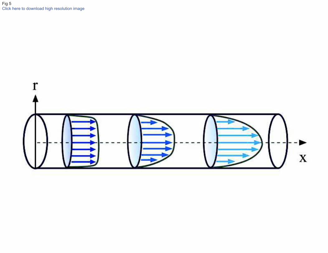
4.2.3 Flow in a straight tube

Figure 5 shows the development of a steady laminar flow in a straight tube. At the entrance of the

tube the velocity profile is almost flat. Due to the no-slip condition, the velocity is zero at the walls

and a velocity gradient is immediately generated with the adjacent moving fluid. As a result of this

traction, high WSS appears on the wall and a viscous boundary layer grows. The boundary layer

progressively decelerates the near-wall fluid, while acceleration occurs at the center of the tube.

The shear stress is gradually reduced on the wall until it becomes constant when the boundary

layer has filled the tube and a parabolic velocity profile has been established. This is the well-

known steady fully-developed laminar flow (Poiseuille flow).

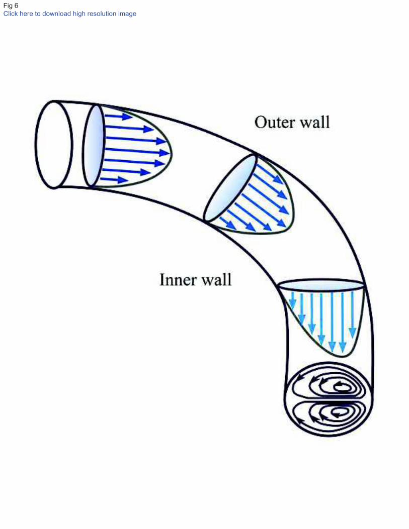
4.2.4 Flow in a curved tube

In order to measure and interpret the flow dynamics in the complex geometry of the human aortic

arch, it is important to understand the effect of curvature on the flow development. In curved tubes

the fluid particles are forced to change direction and accelerate in order to preserve the axial flow.

The large pressure gradient that is developed is what drives this acceleration. If the initial flow is

fully developed, the central highest velocities have high inertia and cannot be easily deflected.

Fluid near the wall has less inertia and therefore is greatly displaced. Consequently, the highest

velocities do not occur in the center but are found closer to the outer wall of the curvature. The

displacement also generates secondary motions in the transverse plane in the form of two counter-

rotating vortices (Dean vortices) moving from the outer bend to the inner bend along the walls of

the tube (Figure 6), as occur when there is a flow around a pipe bend [219]. The skewness of the

velocity profile implies that in a curved tube high shear stress is developed on the outer wall, and

low shear stress on the inner wall.

16

Dean [199,200] developed the analytical solution for a fully developed, steady viscous flow in a

curved tube of circular cross section, and demonstrated that the degree of influence of curvature on

a steady streamlined flow can be expressed by the dimensionless Dean number:

OP = QPB$R (8)

where ! is the tube radius and Q is the radius of curvature. The Dean number is a measure of the

ratio of centrifugal inertial forces to viscous forces, analogous to the definition of the Reynolds

number. With an increasing Dean number, the effects of the centrifugal forces become stronger

and increase the secondary motions. Dean number can be used to assess the variation due to the

radius of curvature effects along the aortic arch.

4.2.5 Flow in a bifurcation

When a steady fluid flow arrives at a bifurcation, it is forced to divide into the branches (Figure 7).

Due to its high inertia, the acting pressure gradient cannot displace it immediately into the axial

directions of the branches and, hence, the flow moves next to the inner walls of the bifurcation.

High shear is developed, as a result, on the flow divider. On the contrary, near-wall fluid in the

parent vessel has less inertia and can be greatly deflected. This generates secondary motions in the

transverse plane, while low shear regions develop on the outer walls of the bifurcation. New

boundary layers develop along the inner walls that eventually reestablish the Poiseuille flow type

in both daughter branches further downstream. At very high initial velocities and sharp angles,

large pressure gradients may cause separation of the flow and the formation of a separation zone or

flow reversal at the outer walls. Such zones are characterized by high particle residence times and

low values of WSS.

5. Post-processing

After the governing equations are solved and the convergence criterion is reached, the simulation

results are analyzed and visualized at different locations and time instants. Additional

hemodynamic parameters of interest computed from the basic flow fields, such as WSS, energy

losses, pressure wave propagation, wall compliance, mass transport phenomena and particle

residence time, are usually interpreted by means of contour and vector plots, streamlines and

particle tracking, or 2D and 3D surface plots. A significant challenge of patient-specific modelling

is making sense of the large amount of numerical data that can—and should—be extracted. Also,

this data must be analyzed at different levels of detail for different purposes; maps of quantities of

biological significance may be of interest to a clinical audience, while other quantities must be

considered if the computational model was integrated with a reduced-order model.

In order to organize in a detailed manner the findings of the TA studies included in this review,

comparative information is provided in tabular format. Table 1 is organized chronologically and

provides the model setup, simulation results and a summary of the major insights and

contributions of each article reviewed. Conference papers were not included. In general, most TA

studies focused on surface-based parameters, which are thought to be most closely linked to the

pathogenesis of different CVDs. WSS, TAWSS and OSI remain the most commonly reported

hemodynamic wall parameters in CFD studies (Figure 8). Traditionally, these quantities have been

presented as spatial maps or trends at a particular spatial location. As TA studies have moved from

idealized to patient-specific cases, several groups have encouraged a more statistical treatment of

these parameters. Besides from surface-related quantities, velocity fields and volumetric

parameters also have much to tell. Velocity iso-contours are ideal for visualizing or quantifying

regions of slow recirculating and retrograde flow at branches. Simulated dye studies are attractive

for visualizing the complexities of pulsatile flows but also for facilitating indirect comparisons

against in vivo image-based data. It is likely that a variety of other quantities -yet to be identified -

will need to be interrogated as new biological mechanisms are identified and new numerical

models are developed to understand them. Discussions between the clinician and the scientist are

then the key to choose such parameters and to interpret the results.

17

5.1 Verification and validation

An acute aspect of CFD hemodynamic studies is their verification and validation. Verification is

defined as the assessment of the numerical accuracy with which the computational model was

implemented. This process usually relies on the existence of an analytical solution for the model.

By contrast, validation is the process of determining the degree to which the computational model

is an accurate representation of the real world, and quantifying its uncertainty. A simulation is

considered to be validated if the differences between its results and experimental data are small

and if the uncertainties in the experimental results are also small [193]. It is clear that when

developing new models for hemodynamic modelling, the verification should precede any attempt

of validation. A clear distinction between verification and validation is given by Roache and

Babuska & Oden [201,202], who describe verification as “solving the equations right”, whereas

validation is “solving the right equations.”

Traditionally, CFD validation studies have primarily used in-vitro models [203-205]. Kung et al.

[206] compared numerical simulations of flow and pressure incorporating deformable walls using

in-vitro flow phantoms under physiological flow and pressure conditions. Regarding in-vivo

validation, relatively few studies have been published comparing patient-specific hemodynamics

simulations with in-vivo measurements [207-209]. Boussel et al. [210] compared CFD data and in

vivo PC-MRI measurements in patient-specific intracranial aneurysms models. They reported

favorable agreement for flow patterns and velocities, but poor agreement for WSS due to the

incapability of PC-MRI to capture near-wall velocity gradients.

To the authors´ knowledge, full validation TA studies comparing patient-specific simulations with

in vivo data have not been published. In [4,5,16,20,21,29] some velocity results were slightly

compared with PC-MRI data measured at different sections of the TA that were not used as

boundary conditions. Though the simulation results reported good qualitative agreement between

computed and PC-MRI in-vivo velocity patterns, this does not show that flow field details are

being correctly predicted, but it does give some assurance and is a first step towards validation.

Although initial results are encouraging, in-vivo validation studies remain in their infancy. PC-

MRI offers the greatest promise as an in-vivo gold standard, but still provides a comforting but

inconclusive evidence that simulations are physiological faithful. In addition, it is likely that

validation studies may require the acquisition of extra data; however, this additional cost is critical

if we are to rely on simulation-based results in the future. In the context of predictive simulations,

establishing a database of experimental results which could act as test cases for research groups

wishing to validate their computational models would be useful, and may call for novel clinical

protocols.

6. Conclusions and future challenges

Over the past decades, computational simulations of blood flow have gained great relevance in

understanding the human cardiovascular system, in particular the origin and development of

different CVDs. The sophistication of the models and the quality of the results has increased

dramatically as the developments in the resolution of medical-imaging data and the performance of

computers has improved significantly. However, as noted previously, this level of sophistication

requires more information than the mere definition of the domain of interest: there is a pressing

need to characterize the mechanical behavior of the vasculatures and the external tissues around it

with patient-specific boundary conditions. It is clear that given the large patient-to-patient

variability of the cardiovascular system, the interactions between the fluid and a solid that is

constrained by external tissues must be defined on a patient-specific basis.

In addition, we must move from computational ‘‘snap-shots’’ focusing on a mechanical state and

on the role of WSS in vascular pathophysiology, to studies focusing on dynamic

mechanobiological processes that encompass the time course of arterial growth and remodelling

(G&R). By growth, we mean a change in mass; by remodelling, we mean a change in structure.

Arteries exhibit a remarkable ability to adapt throughout life: we observe arterial adaptation in

development and aging, adaptations to injury, adaptations in disease, and adaptations to changes in

the overall hemodynamic state of the patient. Arterial diseases are diseases of the arterial wall;

18

hence internal tissue-level stresses affect the normal biologic phenomena in many cases as much

or more than WSS. The main remodelling agents in the arterial wall are the ECs, vascular smooth

muscle cells, and fibroblasts. Many studies have attempted to elucidate the role of each of these

elements in arterial G&R. From a computational standpoint, two main approaches have been

proposed: the kinematic-growth approach [211,212] and the constrained-mixture approach [213-

215]. Although new computational approaches have been recently suggested [216-218], there is a

pressing need to determine whether G&R relations that have hold for modest adaptations would

hold in pathological conditions.

Interventional and surgical therapies used in the treatment of CVDs attempt to restore blood flow

to compromised organs and tissues at no risk to the patient. Ideally, these therapies should result in

sufficient blood flow at appropriate physiologic pressures while avoiding adverse flow conditions

that may lead to procedural failure or poor outcomes. Unfortunately, most of the advances in

surgical techniques and interventions have come about as a result of a trial-and-error design

process. Currently, alternate and new techniques are evaluated by performing the new procedure

on a series of patients, and then evaluating clinical outcomes. Physicians do not have all the tools

needed to evaluate the multiple options and to design the optimal corrective procedures, since

diagnostic imaging, physical measurements, and empirical data are insufficient to predict the

outcome of a given treatment for an individual patient owing anatomic and physiologic variations

and system complexity.

In the new paradigm of predictive medicine, the surgical community would achieve more effective

healthcare from computational tools to construct and evaluate patient-specific

anatomic/physiologic models that could optimize treatment, predict outcomes of surgical

interventions and optimize application of cardiovascular devices. In order to achieve clinical

translation, these models ultimately should exploit patient-specific clinical visualisation modalities

and experimentally obtained material properties in combination with fluid dynamics and solid

mechanics models. Detailed knowledge about physiological (control) mechanisms and

pathophysiological processes is necessary to arrive at clinically relevant decision making tools.

Ultimately, these models should account for processes operating at different time scales, ranging

from transient behaviour of pressure and flow during a cardiac cycle, to effects of altered

physiological demands or therapeutic interventions, through much longer time-scale processes

involving G&R due to disease progression and aging. However, much of our current

understanding of CFD hemodynamics is still explanatory rather than predictive, and this new

frontier in computational modelling has an almost limitless number of open problems to challenge

investigators for many years to come. We hope that this review will stimulate computational

research that will contribute to the continued improvement of casdiovascular health through a

strong interaction and cooperation between engineers and clinicians.

Acknowledgments

A.D. Caballero was supported by the COLCIENCIAS Young Researcher Fellowship.

References

[1] Mori D, Yamaguchi T. 2002a. Computational fluid dynamics modelling and analysis of the

effect of 3-D distortion of the human aortic arch. Comput Methods Biomech Biomed Engin.

5:249–260.

[2] Mori D, Hayasaka T, Yamaguchi T. 2002b. Modelling of the human aortic arch with its major

branches for computational fluid dynamics simulation of the blood flow. JSME. C-45(4):997-1002.

19

[3] Shahcheraghi N, Dwyer HA, Cheer AY, Barakat AI, Rutanganira T. 2002. Unsteady and three-

dimensional simulation of blood flow in the human aortic arch. J Biomech Eng. 124(4):378-87.

[4] Jin S, Oshinski J, Giddens DP. 2003. Effect of wall motion and compliance on flow patterns in

the ascending aorta. J. Biomech. Eng. 125:347–354.

[5] Leuprecht A, Kozerke S, Boesiger P, Perktold K. 2003. Blood flow in the human ascending

aorta: a combined MRI and CFD study. Journal of Engineering Mathematics. 47:387–404.

[6] Kim T, Cheer AY, Dwyer HA. 2004. A simulated dye method for flow visualization with a

computational model for blood flow. J Biomech. 27:1125–1136.

[7] Morris L, Delassus P, Callanan A, Walsh M, Wallis F, Grace P, McGloughlin T. 2005. 3-D

numerical simulation of blood flow through models of the human aorta. J Biomech Eng. 127:767-

775.

[8] Gao F, Watanabe M, Matsuzawa T. 2006. Stress analysis in a layered aortic arch model under

pulsatile blood flow. Biomed. Eng Online. 5:25.

[9] Gao F, Matsuzawa T. 2006. FSI within aortic arch model over cardiac cycle and Influence of

wall stiffness on wall stress in layered wall. Engineering Letters. 13:167-172.

[10] Gao F, Guo Z, Sakamoto M, Matsuzawa T. 2006. Fluid structure interaction within a layered

aortic arch model. Journal of Biological Physics. 32(5):435–454.

[11] Gardhagen R, Renner J, Lanne T, Karlsson M. 2006. Subject specific wall shear stress in the

human thoracic aorta. WSEAS Transaction on Biology and Biomedicine. 3(10):609-614.

[12] Park YJ, Park CY, Hwang CM, Sun K, Min BG. 2007. Pseudo-organ boundary conditions

applied to a computational fluid dynamics model of the human aorta. Comput. Biol. Med.

37(8):1063-1072.

[13] Gao F, Ohta O, Matsuzawa T. 2008. Fluid-structure interaction in layered aortic arch

aneurysm model: assessing the combined influence of arch aneurysm and wall stiffness.

Australas Phys Eng Sci Med. 3(1):32-41.

[14] Lam SK, Fung GSK, Cheng SWK, Chow WK. 2008. A computational study on the

biomechanical factors related to stent-graft models in the thoracic aorta. Med Biol Eng Comput.

46:1129–1138.

[15] Soulis JV, Giannoglou GD, Dimitrakopoulou M, Logothetides S, Mikhailidis D. 2009. Influence

of oscillating flow on LDL transport and wall shear stress in the normal aortic arch. Open

Cardiovasc Med J. 17:128-142.

[16] Renner J, Gardhagen R, Heiberg E, Ebbers T, Loyd D, Länne T, Karlsson M. 2009. A method for

subject specific estimation of aortic wall shear stress. WSEAS Transaction on Biology and

Biomedicine. 6(3):49-57.

[17] Renner J, Loyd D, Lanne T, Karlsson M. 2009. Is a flat inlet profile sufficient for WSS

estimation in the aortic arch?. WSEAS Transactions on Fluid Mechanics. 4(4):148-160.

[18] Kim HJ, Vignon-Clementel IE, Figueroa CA, LaDisa JF Jr, Jansen KE, Feinstein JA, Taylor CA.

2009. On coupling a lumped parameter heart model and a three-dimensional finite element aorta

model. Ann Biomed Eng. 37(11):2153–2169.

20

[19] Liu X, Pu F, Fan Y. 2009. A numerical study on the flow of blood and the transport of LDL in

the human aorta: the physiological significance of the helical flow in the aortic arch. Am J Physiol

Heart Circ Physiol. 297: H163-H170.

[20] Tan FPP, Torii R, Borghi A, Mohiaddin RH, Wood NB, Thom S, Xu XY. 2009. Analysis of flow

patterns in a patient-specific thoracic aortic aneurysm model. Computers and Structures. 87:680-

690.

[21] Wen CY, Yang AS, Tseng LY, Chai JW. 2010. Investigation of pulsatile flow field in healthy

thoracic aorta models. Ann Biomed Eng. 38(2):391-402.

[22] Liu X, Fan YB, Deng XY. 2010. Effect of spiral flow on the transport of oxygen in the aorta: A

numerical study. Ann Biomed Eng. 38:917-926.

[23] Wang X, Li X. 2011. Biomechanical behaviors of curved artery with flexible wall: a numerical

study using fluid-structure interaction method. Comput Biol Med. 41(11):1014-1021.

[24] Wang X, Li X. 2011. Computational simulation of aortic aneurysm using FSI method:

influence of blood viscosity on aneurismal dynamic behaviors. Comput Biol Med. 41(9):812-821.

[25] Liu X, Fan Y, Deng X, Zhan F. 2011. Effect of non-Newtonian and pulsatile blood flow on mass

transport in the human aorta. J Biomech. 44(6):1123-1131.

[26] Crosetto P, Reymond P, Deparis S; Kontaxakis D, Stergiopulos N, Quarteroni A. 2011. Fluid-

structure interaction simulation of aortic blood flow. Computers & Fluids. 43:46-57.

[27] Soulis JV, Fytanidis DK, Papaioannou VC, Styliadis H Giannoglou GD. 2011. Oscillating LDL

accumulation in normal human aortic arch - shear dependent endothelium. Hippokratia. 15:22–

25.

[28] Benim AC, Nahavandi A, Assmann A, Schubert D, Feindt P, Suh SH. 2011. Simulation of blood

flow in human aorta with emphasis on outlet boundary conditions. Appl Math Modell.

35(7):3175-3188.

[29] Lantz J, Renner J, Karlsson M. 2011. Wall shear stress in a subject specific human aorta -

Influence of fluid-structure interaction. Int. J. Appl. Mechanics. 3:759-778.

[30] Tse KM, Chiu P, Lee HP, Ho P. 2011. Investigation of hemodynamics in the development of

dissecting aneurysm within patient-specific dissecting aneurismal aortas using computational

fluid dynamics (CFD) simulations. J Biomech. 44(5):827-836.

[31] Filipovic N, Milasinovic D, Zdravkovic N, Böckler D, von Tengg-Kobligk H. 2011. Impact of

aortic repair based on flow field computer simulation within the thoracic aorta. Comput Methods

Programs Biomed. 101(3): 243-252.

[32] Keshavarz-Motamed Z, Kadem L. 2011. 3D pulsatile flow in a curved tube with coexisting

model of aortic stenosis and coarctation of the aorta. Med Eng Phys. 33(3):315-324.

[33] Olivieri LJ, de Zélicourt DA, Haggerty CM, Ratnayaka K, Cross RR, Yoganathan AP. 2011.

Hemodynamic modelling of surgically repaired coarctation of the aorta. Cardiovasc Eng Technol.

2(4):288-295.

21

[34] LaDisa JF Jr, Figueroa CA, Vignon-Clementel IE, Kim HJ, Xiao N, Ellwein LM, Chan FP, Feinstein

JA, Taylor CA. 2011a. Computational simulations for aortic coarctation: representative results

from a sampling of patients. J Biomech Eng. 133(9):81-89.

[35] LaDisa JF Jr, Dholakia RJ, Figueroa CA, Vignon-Clementel IE, Chan FP, Samyn MM, Cava JR,

Taylor CA, Feinstein JA. 2011b. Computational simulations demonstrate altered wall shear stress

in aortic coarctation patients treated by resection with end-to-end anastomosis. Congenit Heart

Dis. 6(5):432-443.

[36] Gallo D, De Santis G, Negri F, Tresoldi D, Ponzini R, Massai D, Deriu MA, Segers P, Verhegghe

B, Rizzo G, Morbiducci U. 2012. On the use of in vivo measured flow rates as boundary conditions

for image-based hemodynamic models of the human aorta: implications for indicators of

abnormal flow. Ann Biomed Eng. 40(3):729-41.

[37] Lantz J, Karlsson M. 2012. Large eddy simulation of LDL surface concentration in a subject

specific human aorta. J Biomech. 45(3):537-542.

[38] Lantz J, Gardhagen R, Karlsson M. 2012. Quantifying turbulent wall shear stress in a subject

specific human aorta using large eddy simulation. Med Eng Phys. 34(8):1139-1148.

[39] Brown AG, Shi Y, Marzo A, Staicu C, Valverde I, Beerbaum P, Lawford PV, Hose DR. 2012.

Accuracy vs. computational time: translating aortic simulations to the clinic. J Biomech.

45(3):516-523.

[40] Vasava P, Jalali P, Dabagh M, Kolari P. 2012. Finite element modelling of pulsatile blood flow

in idealized model of human aortic arch: Study of hypotension and hypertension. Comp. Math.

Methods in Medicine. doi: 10.1155/2012/861837.

[41] Moireau P, Xiao N, Astorino M, Figueroa CA, Chapelle D, Taylor CA, Gerbeau JF. 2012a.

External tissue support and fluid- structure simulation in blood flows. Biomech Model

Mechanobiol. 11:1–18.

[42] Reymond P, Crosetto P, Deparis S, Quarteroni A, Stergiopulos N. 2012. Physiological

simulation of blood flow in the aorta: Comparison of hemodynamic indices as predicted by 3-D

FSI, 3-D rigid wall and 1-D models. Med Eng Phys.

http://dx.doi.org/10.1016/j.medengphy.2012.08.009.

[43] Coogan JS, Humphrey JD, Figueroa CA. 2012b. Computational simulations of hemodynamic

changes within thoracic, coronary, and cerebral arteries following early wall remodelling in

response to distal aortic coarctation. Biomech Model Mechanobiol. doi: 10.1007/s10237-012-

0383-x.

[44] Coogan JS, Chan FP, LaDisa JF Jr, Taylor CA, Hanley FL, Feinstein JA. 2012a. Computational

fluid dynamic simulations for determination of ventricular workload in aortic arch obstructions. J

Thorac Cardiovasc Surg. doi: 10.1016/j.jtcvs.2012.03.051.

[45] Wendell DC, Samyn MM, Cava JR, Ellwein LM, Krolikowski MM, Gandy KL, Pelech AN,

Shadden SC, LaDisa JF Jr. 2012. Including aortic valve morphology in computational fluid

dynamics simulations: Initial findings and application to aortic coarctation. Med Eng Phys.

http://dx.doi.org/10.1016/j.medengphy.2012.07.015.

[46] Morbiducci U, Ponzini R, Gallo D, Bignardi C, Rizzo G. 2013. Inflow boundary conditions for

image-based computational hemodynamics: impact of idealized versus measured velocity

profiles in the human aorta. J Biomech. 46:102-109.

22

[47] Cardiovascular diseases (CVDs), Fact sheet 317. In: World Health Organization. 2012.

http://www.who.int/mediacentre/factsheets/fs317/en/index.html. Accessed 15 December 2012

[48] Davies PF, Mundel T, Barbee KA. 1995. A mechanism for heterogeneous endothelial

responses to flow in vivo and in vitro. Journal of Biomechanics. 28:1553-1560.

[49] Davies PF, Dewey CF, Bussolari S, Gordon E, Gimbrone MA. 1984. Influence of hemodynamic

forces on vascular endothelial function. In vitro studies of shear stress and pinocytosis in bovine

aortic cells. Journal of Clinical Investigation. 73:1121-1129.

[50] Gimbrone Jr MA, Topper JN, Nagel T, Anderson KR, Garcia-Cardena G. 2000. Endothelial

dysfunction, hemodynamic forces, and atherogenesis. Ann N Y Acad Sci. 902:230–239.

[51] Resnick N, Yahav H, Shay-Salit A, Shushy M, Schubert S, Zilberman LC, Wofovitz E. 2003. Fluid

shear stress and the vascular endothelium: for better and for worse. Prog Biophys Mol Biol.

81(3):177–199.

[52] White CR, Frangos JA. 2007. The shear stress of it all: the cell membrane and

mechanochemical transduction. Phil Trans R Soc B. 362:1459–1467.

[53] Ku DN, Giddens DP, Zarins CK, Glagov S. 1985. Pulsatile flow and atherosclerosis in the

human carotid bifurcation. Positive correlation between plaque location and low oscillating shear

stress. Arteriosclerosis. 5(3):293–302.

[54] Moore J, Xu C, Glagov S, Zarins CK, Ku DN. 1994. Fluid wall shear stress measurements in a

model of the human abdominal aorta: oscillatory behavior and relationship to atherosclerosis.

Atherosclerosis. 110(2):225–240.

[55] Cheng C, Tempel D, van Haperen R, van der Baan A, Grosveld F, Daemen MJ, Krams R, de

Crom R. 2006. Atherosclerotic lesion size and vulnerability are determined by patterns of fluid

shear stress. Circulation. 113(23):2744–2753.

[56] Cecchi E, Giglioli C, Valente S, Lazzeri C, Gensini GF, Abbate R, Mannini L. 2011. Role of

hemodynamic shear stress in cardiovascular disease. Atherosclerosis. 214(2):249-256.

[57] Friedman MH, Deters OJ, Mark FF, Bargeron CB, Hutchins GM. 1983. Arterial geometry

affects hemodynamics. A potential risk factor for athersoclerosis. Arteriosclerosis. 46(2):225-231.

[58] Ku DN. 1997. Blood flow in arteries. Annu Rev Fluid Mech. 29:399-434.

[59] Cunningham KS, Gotlieb AI. 2005. The role of shear stress in the pathogenesis of

atherosclerosis. Lab Invest. 85(1):9–23.

[60] Wahle A, Lopez JJ, Olszewski ME, Vigmostad SC, Chandran KB, Rossen JD, Sonka M. 2006.

Plaque development, vessel curvature, and wall shear stress in coronary arteries assessed by X-

ray angiography and intravascular ultrasound. Med Image Anal. 10(4):615-631.

[61] Bogren HG, Klipstein RH, Firmin DN, Mohiaddin RH, Underwood SR, Rees RS, Longmore DB.

1989. Quantitation of antegrade and retrograde blood flow in the human aorta by magnetic

resonance velocity mapping. Am Heart J. 117(6):1214–1222.

[62] Kilner PJ, Yang GZ, Mohiaddin RH, Firmin DN, Longmore DB. 1993. Helical and retrograde

secondary flow patterns in the aortic arch studied by three-directional magnetic resonance

velocity mapping. Circulation. 88(5):2235-2247.

23

[63] Bogren HG, Mohiaddin RH, Kilner PJ, Jimenez-Borreguero LJ, Yang GZ, Firmin DN. 1997.

Blood flow patterns in the thoracic aorta studied with three-directional MR velocity mapping: the

effects of age and coronary artery disease. J Magn Reson Imaging. 7(5):784–793.

[64] Utepov YY, 1997. Correlation between anatomic parameters of the aorta and manifestations

of atherosclerosis. Bulletin of Experimental Biology and Medicine. 124(8):729-734.

[65] Kleinstreuer C, Hyun S, Buchanan JR Jr, Longest PW, Archie JP Jr, Truskey GA. 2001.

Hemodynamic parameters and early intimal thickening in branching blood vessels. Crit Rev

Biomed Eng. 29:1–64.

[66] Wada S, Karino T. 2002. Theoretical prediction of low-density lipoproteins concentration at

the luminal surface of an artery with a multiple bend. Ann Biomed Eng 30(6):778-791.

[67] Tarbell JM. 2003. Mass transport in arteries and the localization of atherosclerosis. Annu Rev

Biomed Engrg. 5:79–118.

[68] Ross R, Harker L. 1976. Hyperlipidemia and atherosclerosis. Science. 193:1094–1100.

[69] Hoff HF, Wagner WD. 1986. Plasma low density lipoprotein accumulation in aortas of

hypercholesterolemic swine correlates with modifications in aortic glycosaminoglycan

composition. Atherosclerosis. 61:231–236.

[70] Ethier CR. 2002. Computational modelling of mass transfer and links to atherosclerosis.

Annals of Biomedical Engineering. (4):461–471.

[71] Nielsen LB. 1996. Transfer of low density lipoprotein into the arterial wall and risk of

atherosclerosis. Atherosclerosis. 123:1–15.

[72] Santilli SM, Stevens RB, Anderson JG, Payne WD, Caldwell MD. 1995. Transarterial wall

oxygen gradients at the dog carotid bifurcation. American Journal of Physiology. 268: H155–161.

[73] Ogawa S, Gerlach H, Esposito C, Pasagian-Macaulay A, Brett J, Stern D. 1990. Hypoxia

modulates the barrier and coagulant function of cultured bovine endothelium. Increased

monolayer permeability and induction of procoagulant properties. The Journal of Clinical

Investigation. 85: 1090–1098.

[74] Sluimer JC, Gasc JM, van Wanroij JL, Kisters N, Groeneweg M, Sollewijn Gelpke MD, Cleutjens

JP, van den Akker LH, Corvol P, Wouters BG, Daemen MJ, Bijnens AP. 2008. Hypoxia, hypoxia-

inducible transcription factor, and macrophages in human atherosclerotic plaques are correlated

with intraplaque angiogenesis. J Am Coll Cardiol. 51(13):1258–1265.

[75] Okamoto R, Hatani M, Tsukitani M, Suehiro A, Fujino M, Imai N, Takano S, Watanabe Y,

Fukuzaki H. 1983. The effect of oxygen on the development of atherosclerosis in WHHL rabbits.

Atherosclerosis. 47:47–53.

[76] Sumida M, Sudou K, Wada H. 1989. Pulsating Flow in a Curved Pipe-Secondary Flow. JSME

Int J, Ser II. 32(4):523–531.

[77] Hamakiotes CC, Berger SA. 1990. Periodic Flows through Curved Tubes: The Effect of the

Frequency Parameter. J Fluid Mech. 210:353–370.

[78] Naruse T, Tanishita K. 1996. Large Curvature Effect on Pulsatile Flow in a Curved Tube:

Model Experiment Simulating Blood Flow in an Aortic Arch. J Biomech Eng. 118:180–186.

24

[79] Komai Y, Tanishita K. 1997. Fully Developed Intermittent Flow in a Curved Tube. J Fluid

Mech. 347:263–287.

[80] Santamarina A, Weydahl E, Siegel JM, Moore JE. 1998. Computational analysis of flow in a

curved tube model of the coronary arteries: Effects of time-varying curvature. Ann Biomed Eng.

26(6):944-954.

[81] Waters SL, Pedley TJ. 1999. Oscillatory Flow in a Tube of Time- Dependent Curvature. Part 1.

Perturbation to Flow in a Stationary Curved Tube. J Fluid Mech. 383:327–352.

[82] Steinman DA. 2002. Image-based computational fluid dynamics modelling in realistic arterial

geometries. Ann Biomed Eng. 30:483–497.

[83] Taylor CA, Steinman DA. 2010. Image-based modelling of blood flow and vessel wall

dynamics: applications, methods and future directions. Ann Biomed Eng. 38:1188–1203.

[84] Antiga L, Piccinelli M, Botti L, Ene-Iordache B, Remuzzi A, Steinman D. 2008. An image-based

modelling framework for patient-specific computational hemodynamics. Med Biol Eng Comput.

46: 1097–1112.

[85] Bekkers EJ, Taylor CA. 2008. Multiscale vascular surface model generation from medical

imaging data using hierarchical features. IEEE Trans Med Imaging. 27:331–341.

[86] De Santis G, Mortier P, De Beule M, Segers P, Verdonck P, Verhegghe B. 2010. Patient-

specific computational fluid dynamics: structured mesh generation from coronary angiography.

Med Biol Engineering and Computing. 48(4):371-380.

[87] Longest PW, Vinchurkar S. 2007. Effects of mesh style and grid convergence on particle

deposition in bifurcating airway models with comparisons to experimental data. Medical

Engineering & Physics. 29(3):350–366.

[88] Prakash S, Ethier CR. 2001. Requirements for mesh resolution in 3D computational

hemodynamics. J Biomech Eng. 123:134–144.

[89] Roache PJ. 1997. Quantification of uncertainty in computational fluid dynamics. Annu Rev

Fluid Mech. 29:123–160.

[90] Muller J, Sahni O, Li X, Jansen KE, Shephard MS, Taylor CA. 2005. Anisotropic adaptive finite

element method for modelling blood flow. Comput Methods Biomech Biomed Eng. 8:295-305.

[91] Sahni O, Muller J, Jansen KE, Shephard MS, Taylor CA. 2006. Efficient anisotropic adaptive

discretization of the cardiovascular system. Comput Methods Appl Mech Eng. 195:5634-5655.

[92] Sahni O, Jansen KE, Shephard MS, Taylor CA, Beall MW. 2008. Adaptive boundary layer

meshing for viscous flow simulations. Eng Comput. 24:267–285.

[93] Chien S, Usami S, Dellenback RJ, Gregersen MI. 1967. Blood viscosity: Influence of

erythrocyte aggregation. Science. 157:827–829.

[94] Thurston GB. 1972. Viscoelasticity of human blood. Biophys J. 12:1205–1217.

[95] Barbee JH. 1973. The effect of temperature on the relative viscosity of human blood.

Biorheology. 10:1-5.

25

[96] Ohta M, Wetzel SG, Dantan P, Bachelet C, Lovblad KO, Yilmaz H, Flaud P, Rüfenacht DA.

2005. Rheological Changes After Stenting of A Cerebral Aneurysm: A Finite Element Modelling

Approach. Cardiovas Intervent Radiol. 28:768-772.

[97] Ballyk PD, Steinman DA, Ethier CR. 1994. Simulation of non-Newtonian blood flow in an end-

to-end anastomosis. Biorheology. 31(5):565–586.

[98] Cho YI, Kensey KR. 1991. Effects of the non-Newtonian viscosity of blood on flows in a

diseased arterial vessel. Part 1: steady flows. Biorheology. 28:241–262.

[99] Massoudi M, Phuoc TX. 2008. Pulsatile flow of blood using a modified second-grade fluid

model, Comput Math with Appl. 56:199-211.

[100] Gonzalez HA, Moraga NO. 2005. On Predicting Unsteady Non-Newtonian Blood Flow. App

Math Comp. 170:909-923.

[101] Sankar DS, Hemalatha K. 2007. Pulsatile flow of Herschel–Bulkley fluid through catheterized

arteries - A mathematical model. Appl Math Model. 31:1497-1517.

[102] Owens RG. 2006. A new microstructure-based constitutive model for human blood. J Non-

Newton Fluid Mech. 140:57–70.

[103] Zaman G, Islam S, Kang YH, Jung H. 2012. Blood flow of an Oldroyd-B fluid in a blood vessel

incorporating a Brownian stress. Sci China Phys Mech Astron. 55:125–131.

[104] Pedley TJ. 1980. The Fluid Mechanics of Large Blood Vessels. Cambridge University Press,

Cambridge.

[105] Liepsch D. 2002. An introduction to biofluid mechanics—basic models and applications. J

Biomech. 35:415–435.

[106] Johnston BM, Johnston PR, Corney S, Kilpatrick D. 2004. Non-Newtonian blood flow in

human right coronary arteries: steady state simulations. J Biomech. 37:709–720.

[107] Chen J, Lu XY. 2006. Numerical investigation of the non-Newtonian pulsatile blood flow in a

bifurcation model with a non-planar branch. J Biomech. 39:818–832.

[108] Johnston BM, Johnston PR, Corney S, Kilpatrick D. 2006. Non-newtonian blood flow in

human right coronary arteries: Transient simulations. J Biomech. 39:1116-1128.

[109] Boyd J, Buick JM. 2007. Comparison of Newtonian and non-Newtonian flows in a two-

dimensional carotid artery model using the lattice Boltzmann method. Phys in Med and Biol. 52:

6215-6228.

[110] Holzapfel GA, Ogden RW. 2006. Mechanics of biological tissue. Springer-Verlag.

[111] Perktold K, Rappitsch G. 1995. Computer simulation of local blood flow and vessel

mechanics in a compliant carotid artery bifurcation model. J Biomech. 28:845–856.

[112] Hofer M, Rappitsch G, Perktold K., Trubel W, Schima H. 1996. Numerical study of wall

mechanics and fluid dynamics in end-to-side anastomoses and correlation to intimal hyperplasia.

J Biomech. 29:1297–1308.

[113] Prosi M, Perktold K, Ding ZH, Friedman MH. 2004. Influence of curvature dynamics on

pulsatile coronary artery flow in a realistic bifurcation model. J Biomech. 37:1767–1775.

26

[114] Deparis S, Fernandez MA, Formaggia L. 2003. Acceleration of a fixed point algorithm for

fluid-structure interaction using transpiration conditions. Math Model Numer Anal. 37(4): 601-

616.

[115] Fernandez MA, Le Tallec P. 2003. Linear stability analysis in fluid-structure interaction with

transpiration. Part II: Numerical analysis and applications. Comput Methods Appl Mech Engrg.

192: 4837-4873.

[116] Figueroa CA, Vignon-Clementel IE, Jansen KE, Hughes TJR, Taylor CA. 2006. A coupled

momentum method for modelling blood flow in three-dimensional deformable arteries. Comput

Methods Appl Mech Engrg. 195:5685-5706.

[117] Peskin CS. 2002. The immersed boundary method. Acta Numer. 11:479–517.

[118] Kim Y, Lim S, Raman SV, Simonetti OP, Friedman A. 2009. Blood flow in a compliant vessel

by the immersed boundary method. Ann Biomed Eng. 37(5):927–942.

[119] Hughes TJR, Liu WK, Zimmermann TK. 1981. Lagrangian–Eulerian finite element formulation

for incompressible viscous flows. Comput Methods Appl Mech Eng. 29:329–349.

[120] Donea J, Giuliani S, Halleux JP. 1982. An arbitrary Lagrangian-Eulerian finite element

method for transient dynamic fluid-structure interactions. Comput Methods Appl Mech Engrg.

33:689-723.

[121] Segers P, Stergiopulos N, Westerhof N, Wouters P, Kolh P, Verdonck P. 2003. Systemic and

pulmonary hemodynamics assessed with a lumped-parameter heart arterial interaction model. J

Eng Math. 47(3):185–199.

[122] Formaggia L, Lamponi D, Tuveri M, Veneziani A. 2006. Numerical modelling of 1D arterial

networks coupled with a lumped parameters description of the heart. Comput Meth Biomech

Biomed Eng. 9(5):273–288.

[123] Hunter PJ, Pullan AJ, Smaill BH. 2003. Modeling total heart function. Annu Rev Biomed Eng.

5:147–177.

[124] Peskin CS. 1972. Flow patterns around heart valves: a numerical method. J Comput Phys.

10:252–271.

[125] Peskin CS. 1977. Numerical analysis of blood flow in the heart. J Comput Phys. 25:220–252.

[126] McQueen DM, Peskin CS. 2000. A three-dimensional computer model of the human heart

for studying cardiac fluid dynamics. SIGGRAPH Computer Graphics. 34:56–60.

[127] Griffith BE. 2012. Immersed boundary model of aortic heart valve dynamics with

physiological driving and loading conditions. Int J Numer Meth Biomed Eng. 28:317–345.

[128] Krittian S, Janoske U, Oertel H, Bhlke T. 2010. Partitioned fluid–solid coupling for

cardiovascular blood flow. Ann Biomed Eng. 38:1426–1441.

[129] Nordsletten D, Niederer S, Nash M, Hunter P, Smith N. 2011. Coupling multi-physics models

to cardiac mechanics. Prog Biophys Mol Biol. 104:77–88.

[130] Taylor CA, Figueroa CA. 2009. Patient-specific modelling of cardiovascular mechanics. Annu

Rev Biomed Eng. 11:109-34.

27

[131] Seed WA, Wood NB. 1971. Velocity Patterns in the Aorta. Cardiovasc Res. 5:319–330.

[132] Falsetti H, Kiser KM, Francis GP, Belmore ER. 1972. Sequential Velocity Development in the

Ascending and Descending Aorta of the Dog. CircRes. 21:328–338.

[133] Nerem RM, Rumberger JA, Gross DR, Hamlin RL, Geiger GL. 1974. Hot-Film Anemometry

Velocity Measurements of Arterial Blood Flow in Horses. CircRes. 10:301–313.

[134] Morbiducci U, Ponzini R, Rizzo G, Cadioli M, Esposito A, Montevecchi FM, Redaelli A. 2011.

Mechanistic insight into the physiological relevance of helical blood flow in the human aorta. An

in vivo study. Biomech Model Mechanobiol. 10: 339–355.

[135] Kern MJ, Lim MJ, Goldstein JA. 2009. Hemodynamic Rounds: Interpretation of Cardiac

Pathophysiology from Pressure Waveform Analysis Transport Phenomena in the Cardiovascular

System. 3rd ed. Wiley-Blackwell.

[136] Myers JG, Moore JA, Ojha M, Johnston KW, Ethier CR. 2001. Factors Influencing Blood Flow

Patterns in the Human Right Coronary Artery. Ann Biomed. Eng. 29(2):109–120.

[137] Moyle KR, Antiga L, Steinman DA. 2006. Inlet conditions for image-based CFD models of the

carotid bifurcation: Is it reasonable to assume fully developed flow?. J Biomech Eng. 128(3):371-

379.

[138] Morris L, Delassus P, Grace P, Wallis F, Walsh M, McGloughlin T. 2006. Effects of flat,

parabolic and realistic steady flow inlet profiles on idealised and realistic stent graft fits through

abdominal aortic aneurysms (AAA). Med Eng Phys. 28:19-26.

[139] Campbell IC, Ries J, Dhawan SS, Quyyumi AA, Taylor WR, Oshinski JN. 2012. Effect of inlet

velocity profiles on patient-specific computational fluid dynamics simulations of the carotid

bifurcation. J Biomech Eng. 134(5):151001-8.

[140] Taylor CA, Hughes TJR, Zarins CK. 1998. Finite element modelling of blood flow in arteries.

Comput Methods Appl Mech Engrg. 158:155-196.

[141] Oshima M, Torii R, Kobayashi T, Taniguchi N, Takagi K. 2001. Finite element simulation of

blood flow in the cerebral artery. Comput Methods Appl Mech Engrg. 191:661-671.

[142] Van de Vosse FN, de Hart J, van Oijen CHGA, Bessems D, Segal A, Wolters BJBM, Stijnen,

Baaijens FPT. 2003. Finite-element-based computational methods for cardiovascular fluid-

structure interaction. J Eng Math. 47:335-368.

[143] Gerbeau JF, Vidrascu M, Frey P. 2005. Fluid-structure interaction in blood flows on

geometries based on medical imaging. Comput Struct. 83:155-165.

[144] Middleman S. 1972. Transport Phenomena in the Cardiovascular System. 1st ed. John Wiley

and Sons.

[145] Murray CD. 1926. The physiological principle of minimum work: 1. The vascular system and

the cost of blood volume. Proc Natl Acad Sci. 12:207-214.

[146] Taylor CA, Cheng CP, Espinosa LA, Tang BT, Parker D, Herfkens RJ. 2002. In vivo

quantification of blood flow and wall shear stress in the human abdominal aorta during lower

limb exercise. Ann Biomed Eng.30:402–408.

28

[147] Bove EL, de Leval MR, Migliavacca F, Guadagni G, Dubini G. 2003. Computational

fluid dynamics in the evaluation of hemodynamic performance of cavopulmonary connections

after the Norwood procedure for hypoplastic left heart syndrome. J Thorac Cardiovasc Surg.

126(4):1040-1047.

[148] Migliavacca F, Dubini G, Bove EL, de Leval MR. 2003. Computational fluid dynamics

simulations in realistic 3-D geometries of the total cavopulmonary anastomosis: the influence of

the inferior caval anastomosis. J Biomech Eng. 125(6):805–813.

[149] Vignon-Clementel IE, Figueroa CA, Jansen KE, Taylor CA. 2006.Outflow boundary conditions

for three-dimensional finite element modelling of blood flow and pressure in arteries. Comput

Methods Appl Mech Eng. 195:3776–3796.

[150] Shi Y, Lawford P, Hose R. 2011. Review of zero-D and 1-D models of blood flow in the

cardiovascular system. BioMedical Engineering OnLine. 10:1-38.

[151] Formaggia L, Gerbeau JF, Nobile F, Quarteroni A. 2001. On the coupling of 3D and 1D

Navier–Stokes equations for flow problems in compliant vessels. Comput Methods Appl Mech

Eng. 191: 561–582.

[152] Urquiza SA, Blanco PJ, Venere MJ, Feijoo RA. 2006. Multidimensional modelling for the

carotid artery blood flow. Comput Meth Appl Mech Eng. 195:4002–4017.

[153] Blanco PJ, Feijoo RA, Urquiza SA. 2007. A unified variational approach for coupling 3D-1D

models and its blood flow applications. Comput Meth Appl Mech Eng. 196:4391-4410.

[154] Papadakis G. 2009. Coupling 3D and 1D fluid-structure-interaction models for wave

propagation in flexible vessels using a finite volume pressure-correction scheme. Commun

Numer Methods Eng. 25(5):533–551.

[155] Olufsen MS, Peskin CS, Kim WY, Pedersen EM, Nadim A, Larsen J. 2000. Numerical

simulation and experimental validation of blood flow in arteries with structured-tree outflow

conditions. Ann Biomed Eng. 28(11):1281–1299.

[156] Steele BN, Olufsen MS, Taylor CA. 2007. Fractal network model for simulating abdominal

and lower extremity blood flow during resting and exercise conditions. Comput Methods

Biomech Biomed Eng. 10:39–51.

[157] Sherwin SJ, Blackburn HM. 2005. Three-dimensional instabilities and transition of steady

and pulsatile axisymmetric stenotic flows. J Fluid Mech. 533:297–327.

[158] Migliavacca F, Dubini G, de Leval M. 2000. Computational fluid dynamics in paediatric

cardiac surgery. Images Paediatr Cardiol. 2:11–25.

[159] Lagana K, Balossino R, Migliavacca F, Pennati G, Bove EL, de Leval MR, Dubini G. 2005.

Multiscale modelling of the cardiovascular system: application to the study of pulmonary and

coronary perfusions in the univentricular circulation. J Biomech. 38:1129–1141.

[160] Bazilevs Y, Gohean JR, Hughes TJR, Moser RD, Zhang Y. 2009. Patient- specific isogeometric

fluid-structure interaction analysis of thoracic aortic blood flow due to implantation of the Jarvik

2000 left ventricular assist device. Comput Methods Appl Mech Eng. 198:3534–3550.

[161] Spilker RL, Taylor CA. 2010. Tuning multidomain hemodynamic simulations to match

physiological measurements. Ann Biomed Eng. 38:2635–2648.

29

[162] Quarteroni A, Ragni S, Veneziani A. 2001. Coupling between lumped and distributed models

for blood flow problems. Comput Vis Sci. 4(2):111–124.

[163] Quarteroni A, Veneziani A. 2003. Analysis of a geometrical multiscale model based on the

coupling of ODEs and PDEs for blood flow simulations. Multiscale Model Simul. 1(2):173–195.

[164] Vignon-Clementel IE, Figueroa CA, Jansen KE, Taylor CA. 2010. Outflow boundary conditions

for three-dimensional simulations of non-periodic blood flow and pressure fields in deformable

arteries. Computer Methods in Biomechanics & Biomedical Engineering. 13:625-640.

[165] Hughes TJR, Lubliner J. 1973. On the one-dimensional theory of blood flow in the larger

vessels. Math. Biosci. 18:161-170.

[166] Cohen IM, Kundu PK. 2004. Fluid mechanics. 3ed. Cambridge University Press, New York.

[167] Formaggia L, Moura A, Nobile F. 2007. On the stability of the coupling of 3D and 1D fluid-

structure interaction models for blood flow simulations. M2AN Math Model Numer Anal.

41(4):743–769.

[168] Quarteroni A. 2009. Numerical models for differential problems. 1st ed. Modelling,

simulation and applications. Springer.

[169] Liu Y, Dang C, Garcia M, Gregersen H, Kassab GS. 2008. Surrounding tissues affect vessel

mechanics. AJP – Heart Circ Physiol. 294:514–523.

[170] Moireau P, Bertoglio C, Xiao N, Figueroa CA, Taylor CA, Chapelle D, Gerbeau JF. 2012b.

Sequential Identification of Boundary Support Parameters in a Fluid-Structure Vascular Model

using Patient Data. Biomech Model Mechanobiol. doi: 10.1007/s10237-012-0418-3.

[171] Blum J, Le Dimet FX, Navon IM. 2009. Data assimilation for geophysical fluids. Comput

Methods Atmos Oceans. 14:385–441.

[172] Navon IM. 2009. Data assimilation for atmospheric, oceanic, hydrologic applications.

Springer, Berlin. Data assimilation for numerical weather prediction: a review, 21-65.

[173] Nerem RM, Seed WA, Wood NB. 1972. An experimental study of the velocity distribution

and transition to turbulence in the aorta. J Fluid Mech. 52:137–160.

[174] Fung YC. 1990. Biomechanics, Motion, Flow, Stress, and Growth. Springer-Verlag.

[175] Liepsch D, Moravec S, Baumgart R. 1992. Some flow visualization and laser-doppler velocity

measurements in a true-to-scale elastic model of a human aortic arch – a new model technique.

Biorheology. 29:563–580.

[176] Fung YC. 1997. Biomechanics Circulation. 2nd ed. Springer.

[177] Hart JD. 1997. Nonparametric Smoothing and Lack-of-Fit Tests. 1st ed. Springer-Verlag.

[178] Morbiducci U, Ponzini R, Rizzo G, Cadioli M, Esposito A, De Cobelli F, Del Maschio A,

Montevecchi FM, Redaelli A. 2009. In vivo quantification of helical blood flow in human aorta by

time-resolved three-dimensional cine phase contrast magnetic resonance imaging. Ann Biomed

Eng. 37:516–531.

30

[179] Stalder AF, Frydrychowicz A, Russe MF, Korvink JG, Hennig J, Li K, Markl M. 2011.

Assessment of flow instabilities in the healthy aorta using flow-sensitive MRI. J Magn Reson

Imaging. 33:839–846.

[180] Stein PD, Sabbah HN. 1976. Turbulent blood flow in the ascending aorta of humans with

normal and diseased aortic valves. Circ. Res. 39:58–65.

[181] Peacock J, Jones T, Tock C, Lutz R. 1998. The onset of turbulence in physiological pulsatile

flow in a straight tube. Experiments in Fluids. 24:1–9.

[182] Varghese SS, Frankel SH. 2003. Numerical modelling of pulsatile turbulent flow in stenotic

vessels. J Biomech Eng. 125:445–460.

[183] Ryval J, Straatman AG, Steinman DA. 2004. Two-equation turbulence modelling of pulsatile

flow in a stenosed tube. J Biomech Eng. 126:625–635.

[184] Banks J, Bressloff NW. 2007. Turbulence modelling in three-dimensional stenosed arterial

bifurcations. J Biomech Eng. 129:40–50.

[185] Yoganathan AP, Chandran KB, Sotiropoulos F. 2005. Flow in prosthetic heart valves: state-

of-the-art and future directions. Ann Biomed Eng. 33:1689–1694.

[186] Varghese SS, Frankel SH, Fischer PF. 2008. Modelling transition to turbulence in eccentric

stenotic flows. J Biomech Eng. 130:014503.

[187] Paul MC, Mamun Molla M, Roditi G. 2009. Large-Eddy simulation of pulsatile blood flow.

Med Eng Phys. 31:153–159.

[188] Gardhagen R, Lantz J, Carlsson F, Karlsson M. 2010. Quantifying turbulent wall shear stress

in a stenosed pipe using large eddy simulation. J Biomech Eng. 132:061002.

[189] Tan FPP, Wood NB, Tabor G, Xu XY. 2011. Comparison of LES of steady transitional flow in

an idealized stenosed axisymmetric artery model with a RANS transitional model. J Biomech Eng.

133: 051001.

[190] Antiga L, Steinman DA. 2009. Rethinking turbulence in blood. Biorheology. 46:77–81.

[191] Wang CY. 1991. Exact solutions of the steady-state Navier-Stokes equations. Annu Rev Fluid

Mech. 23:159-177.

[192] Narang BS. 1983. Exact solution for entrance region flow between parallel plates. Int J Heat

Fluid Fl. 4:177-181.

[193] Versteeg HK, Malalasekera W. 2007. An introduction to computational fluid dynamics: the

finite volume method. 2nd ed. Pearson Education Limited.

[194] Caro CG, Pedley TJ, Schroter RC, Seed WA. 1978. The mechanics of the circulation. Oxford

University Press.

[195] Parker KH, Caro CG. 1993. Magnetic Resonance Angiography, Concepts and Applications.

Mosby, St. Louis. Chapter 6, Flow in the macrocirculation: basic concepts from fluid mechanics.

[196] He X, Ku D. 1996. Pulsatile flow in the human left coronary artery bifurcation. J Biomech

Eng. 118:74–82.

31

[197] Womersley JR. 1955. Method for the calculation of velocity, rate of flow and viscous drag in

arteries when the pressure is known. J Physiol. 127:553–563.

[198] Caro CG, Parker KH, Fish PJ, Lever MJ. 1985. Blood flow near the arterial wall and arterial

disease. Clin Hemorheol. 5(6):849–871.

[199] Dean WR. 1927. Note on the motion of fluid in a curved pipe. Phil Mag. 4:208-223.

[200] Dean WR. 1928. The stream-line motion of fluid in a curved pipe. Phil Mag. 5:673-695.

[201] Roache PJ. 1998. Verification and Validation in Computational Science and Engineering.

Hermosa Publishers, Albuquerque NM.

[202] Babuska I, Oden JT. 2004. Verification and validation in computational engineering and

science: basic concepts. Comput Meth Appl Mech Eng. 193:4057–4066.

[203] Ku JP, Elkins CJ, Taylor CA. 2005. Comparison of CFD and MRI flow and velocities in an in

vitro large artery bypass graft model. Ann Biomed Eng. 33(3):257–269.

[204] Ford MD, Stuhne GR, Nikolov HN, Habets DF, Lownie SP, Holdsworth DW, Steinman DA.

2008. PIV-measured versus CFD-predicted flow dynamics in anatomically realistic cerebral

aneurysm models. J Biomech Eng. 130(2):021015.

[205] Kung EO, Les AS, Medina F, Wicker RB, McConnell MV, Taylor CA. 2011a. In vitro validation

of finite element model of AAA hemodynamics incorporating realistic outlet boundary conditions.

J Biomech Eng. 133(4):041003.

[206] Kung EO, Les AS, Figueroa CA, Medina F, Arcaute K, Wicker RB, McConnell MV, Taylor CA.

2011b. In vitro validation of finite element analysis of blood flow in deformable models. Ann

Biomed Eng. 39:1947–1960.

[207] Ku JP, Draney MT, Arko FR, Lee WA, Chan FP, Pelc NJ, Zarins CK, Taylor CA. 2002. In vivo

validation of numerical prediction of blood flow in arterial bypass grafts. Ann Biomed Eng.

30(6):743–752.

[208] Ford MD, Nikolov HN, Milner JS, Lownie SP, DeMont EM, Kalata W, Loth F, Holdsworth DW,

Steinman DA. 2005. Virtual angiography for visualization and validation of computational models

of aneurysm hemodynamics. IEEE Trans Med Imaging. 24(12):1586–1592.

[209] Rayz VL, Boussel L, Acevedo-Bolton G, Martin AJ, Young WL, Lawton MT, Higashida R,

Saloner D. 2008. Numerical simulations of flow in cerebral aneurysms: comparison of CFD results

and in vivo MRI measurements. J Biomech Eng. 130(5):051011.

[210] Boussel L, Rayz V, Martin A, Acevedo-Bolton G,. Lawton MT, Higashida R, Smith WS,. Young

WL, Saloner D. 2009. Phase-contrast magnetic resonance imaging measurements in intracranial

aneurysms in vivo of flow patterns, velocity fields, and wall shear stress: comparison with

computational fluid dynamics. Magn Reson Med. 61(2):409–417.

[211] Rachev A, Stergiopulos N, Meister JJ. 1998. A model for geometric and mechanical

adaptation of arteries to sustained hypertension. J Biomech Eng. 120:9–17.

[212] Taber LA. 1998. A model of aortic growth based on fluid shear and fiber stresses. J Biomech

Eng. 120:348–354.

32

[213] Humphrey JD, Rajagopal KR. 2002. A constrained mixture model for growth and

remodelling of soft tissues. Math Model Methods in Appl Sci. 12:407–430.

[214] Watton PN, Hill NA, Heil M. 2004. A mathematical model for the growth of the abdominal

aortic aneurysm. Biomech. Model. Mechanobiol. 3:98–113.

[215] Kuhl E, Holzapfel GA. 2007. A continuum model for remodelling in living structures. J.

Mater. Sci. 42:8811–8823.

[216] Machyshyn IM, Bovendeerd PHM, van de Ven AAF, Rongen PMJ, van de Vosse FN. 2010. A

model for arterial adaptation combining microstructural collagen remodelling and 3D tissue

growth. Biomech Model Mechanobiol. 9:671–687.

[217] Sheidaei A, Hunley SC, Zeinali-Davarani S, Raguin LG, Baek S. 2011. Simulation of abdominal

aortic aneurysm growth with updating hemodynamic loads using a realistic geometry. Med Eng

Phys. 33:80–88.

[218] Wilson JS, Baek S, Humphrey JD. 2012. Importance of initial aortic properties on the

evolving regional anisotropy, stiffness, and wall thickness of human abdominal aortic aneurysms.

J R Soc Interface. doi: 10.1098/rsif.2012.0097

[219] Laín S, Sommerfeld M. 2013. Characterisation of pneumatic conveying systems using the

Euler/Lagrange approach. Powder Technology. 235:764-782.

Fig. 1 MRI data at maximum intensity projection (a), Patient-specific TA coarctation 3D model (b),

and unstructured mesh with five prism layers adjacent to the arterial wall (c) (Open Source

Medical Software Corporation. http://www.vascularmodel.org)

Fig. 2 Inlet velocity pulsatile waveform at ascending aorta

Fig. 3 Schematic drawing delineating blood flow patterns in TA during early systole (a), mid-to-

late systole (b), and end systole and diastole (c) (Copy from Kilner et al., 1993)

Fig. 4 Different scales of modelling

Fig. 5 Development of steady laminar flow at the entrance of a straight tube (Reproduced after

Caro et al., 1985)

Fig. 6 Steady flow in a curved tube with the presence of skewed axial velocity profile and

secondary motions (Reproduced after Caro et al., 1985)

Fig. 7 Steady flow in a bifurcation with a separation zone, secondary flow, and skewed axial

profile (Reproduced after Caro et al., 1985)

Fig. 8 Example of WSS (Pa) distribution in a healthy TA 3D model in steady state simulation

Table 1 Summary of the major insights and contributions of each TA article

Table 1. Summary of the major insights and contributions of each TA article

B. Conditions

[ ] Geometry Blood A.

Wall Inlet Outlet Time Flow Simulation Results Major Insights and Contributions

1 I-M Water R FV-SW Z B L WSS, velocity First study that used an idealized MRI-based TA geometric model (no

arch branches)

2 I-M Water R FV Z S L WSS, velocity First study that used an idealized MRI-based TA geometric model with

arch branches

3 I-C N R FV-PW O U L WSS, velocity, tracer

distribution, pressure

A passive scalar (tracer) was used to visualize the pulsatile blood flow.

First detailed TA study

4 P-M N FSI MV MV+O U L WSS, velocity

First study that used a patient-specific TA geometric model. Radial

expansion-contraction and translational motion in the ascending aorta was

prescribed. Rigid wall elsewhere. Measured velocity at descending aorta,

outflow at branches. Comparison with MRI data measured at ascending

aorta

5 P-M N ALE MV Z U L WSS, velocity

Study only considered the ascending aorta geometry. Comparison

between blood flow distal to an artificial heart valve and native flow of a

healthy patient. Comparison with MRI data measured at aortic arch

6 I-C N R FV-PW O U L

Womersley number,

Schmidt number, tracer

distribution, velocity

Tracer visualization method was analyzed in more detail compared to [3]

7 I-C N R FV-PW B L Velocity, WSS Three TA geometric model variations were simulated (no arch branches)

8 I N ALE FV-PW Z U L Pressure, wall stress

distribution

First full FSI study. A three-layered TA model (no arch branches) was

used to study the influence of medial wall stiffness on wall stress

distribution

9 I N ALE FV-PW Z U L

Pressure, wall stress

distribution, velocity, wall deformation

Blood flow dynamics was analyzed in more detail compared to [8]

10 I N ALE FV Z S L

Velocity, pressure, WSS,

wall deformation, wall stress

distribution

Blood flow dynamics was analyzed under steady flow conditions

11 P-M N R MV+ PV-

PW O U L WSS, velocity

Two velocity inlet boundary conditions were simulated to compare the

WSS distribution

12 I N R MP - U L Pressure, velocity

Pseudo-organs were connected at outlets. Power Law permeability

functions derived from 2D computations were used in 3D simulations as

outlet boundary conditions

13 I N ALE FV Z S L Pressure, velocity, wall

stress distribution

A three-layered healthy and diseased TA models (no arch branches) were

used to investigate the combined effects of arch aneurysm and medial

wall stiffness on wall stress distribution

14 I N R FV-PW PP U L Velocity, drag force Study investigated the hemodynamics factors affecting the drag force on a stent-graft TA model (no arch branches)

15 I Pl R FV-PW O U L WSS, LDL, velocity, strain

rate, molecular viscosity

First detailed mass transport study. The influence of pulsatile flow on

LDL transport and WSS was analyzed

16 P-M N R MV O U L WSS, velocity

Blood flow of nine healthy patients was simulated. Patient-specific

viscosities were measured. Comparison with MRI data measured at

ascending aorta

17 P-M N R MV+ FV-

PW O U L WSS, velocity

Two velocity inlet boundary conditions were simulated to compare the

WSS distribution

18 P-M N CMM 0D 0D U L Pressure, velocity, WSS,

OSI

Detailed multiscale study investigated blood flow dynamics in a healthy

TA model under rest and exercise conditions, and a in a TA coarctation

model under pre and post-intervention

19 P-M N R FV O S L Velocity, LDL, WSS Four TA geometric model variations were simulated to assess the

influence of helical blood flow on LDL transport

20 P-M N R MV Z+O U L+

SST

Velocity, TAWSS, OSI,

turbulence level

Detailed study investigated laminar and transitional blood flow on a TA

aneurysm model. Zero pressure at descending aorta, outflow at branches.

Comparison with MRI data measured at descending aorta

21 I N R MV MP U L Velocity, pressure, WSS, OSI

Study investigated the relationship between aortic dissection and blood flow dynamics. In-vitro flow rate and pressure data was used as boundary

conditions. Comparison with MRI data measured at different locations

22 P-M N R FV O S L Helicity density, Sherwood

number, hemoglobin, WSS

Three TA geometric model variations were simulated to assess the

influence of helical blood flow on oxygen transport

23 I N ALE FV-PW PP U L Von Mises stress, velocity,

wall deformation

Three TA geometric model variations (no arch branches) were simulated to assess the influence of curvature and flexibility on the wall Von Mises

stress

24 I N ALE FV-PW PP U L Velocity, strain rate, WSS, wall deformation

An aneurysm TA model (no arch branches) was used to investigate the combined effects of FSI and different viscosities on blood flow dynamics

25 P-M N +

Ca R FV-PW - B L

Helicity density, OSI,

Sherwood number, WSS

Detailed study investigated the effect of both non-Newtonian and

pulsatile blood flow on LDL and oxygen transport

26 P-M N R+

ALE

1D

1D

U L WSS, velocity, pressure,

wall deformation

Study investigated the effect of different sets of boundary conditions.

Pressure and flow rate data obtained from 1D simulations was imposed as

boundary conditions. An arterial wall boundary condition was considered

27 I Pl R FV-PW O U L LDL Study examined the LDL accumulation in the aortic wall with shear

dependent endothelium properties

28 I N R FV-PW - B SST Velocity, WSS, wall stress

distribution, turbulence level

Study investigated blood flow dynamics for physiologic and

extracorporeal circulation, the latter being the main focus. A model based

on the prescription of loss coefficients was used as outlet boundary

conditions

29 P-M N R+

CMM MV 0D+O U SST

Velocity, pressure-volume

relation, TAWSS, OSI, WSS

Detailed comparison between FSI and a rigid-wall TA models. Lumped

parameter model coupled to the descending aorta, outflow at branches. A

physiological range of different wall stiffnesses was simulated.

Comparison with MRI data measured at descending aorta

30 P-C N R FV-PW PP+O U L Velocity, pressure, TAWSS

Study investigated blood flow dynamics on pre-aneurysmal and post-

aneurysmal dissecting TA models. Pressure at descending aorta, outflow

at branches

31 P-C N R MV Z+MV U L Velocity, TAWSS, OSI

Study investigated blood flow dynamics on pre-aneurysmal and post-

aneurysmal TA models. Zero pressure at descending aorta, measured

velocities at branches

32 Curved

tube N R FV-PW Z B

L+

SST

Velocity, WSS, pressure,

OSI

Study investigated the effect of different severities of TA coarctation and

stenosis on blood flow dynamics

33 P-M N R FV O S SST WSS, velocity Study investigated blood flow dynamics on a coarctation and three post-

coarctation TA models

34 P-M N CMM MV 0D U L Velocity, TAWSS, OSI,

wall deformation

Study investigated blood flow dynamics on a healthy and four coarctation

TA models under rest and exercise conditions. An arterial wall boundary

condition was considered

35 P-M N R MV 0D U L TAWSS, OSI, velocity Study investigated blood flow dynamics on healthy and post-surgical

coarctation TA models

36 P-M N R MV MV U L Velocity, OSI, TAWSS,

RRT

Detailed study investigated the effect of different sets of outlet boundary

conditions obtained from in-vivo measured flow rates. Measured velocity

at descending aorta, six treatment schemes at branches

37 P-M N R MV 0D+ MV U LES WSS, LDL, velocity

First mass transport study that used a patient-specific TA model. It was

investigated how the LDL surface concentration change during a cardiac

cycle. Lumped parameter model coupled to the descending aorta,

measured velocities at branches

38 P-M N R MV 0D+ MV U LES WSS, velocity, TAWSS,

OSI

A decomposition similar to Reynolds decomposition was introduced to

understand how WSS affects the TA wall

39 P-M N R+FSI FV-PW 0D U L Pressure, mass flow rate,

WSS, helical flow index

Study investigated blood flow dynamics on FSI, compressible fluid and

rigid wall TA models

40 I N R PP PP U L Velocity, pressure, WSS

Two TA geometric model variations were simulated to assess the

influence of hypotension and hypertension pressure conditions on blood

flow dynamics

41 P-C N ALE+

CMM MV 0D U L

2D contour comparison,

wall deformation

Two geometric model variations were simulated, using a distinct FSI

technique for each. An arterial wall boundary condition was considered

42 P-M N R+

ALE

1D

1D

U L WSS, TAWSS, velocity,

pressure, wall deformation

Detailed comparison between FSI and a rigid-wall TA model. Pressure

and flow rate data obtained from 1D simulations was imposed as

boundary conditions. An arterial wall boundary condition was considered

43 P-C N CMM 0D 0D U L Pressure, velocity, cardiac

workload

Study investigated blood flow dynamics on various aortic arch

obstructions models. The hemodynamic significance of aortic coarctation

and various types of aortic hypoplasia to calculate the cardiac workload was determined

44 P-C N CMM 0D 0D U L Pressure, velocity, cyclic

wall strain

Detailed study investigated local and systemic effects on blood flow

dynamics within the TA and coronary, carotid, and cerebral arteries due

to aortic coarctation and spatial variations in wall adaptation

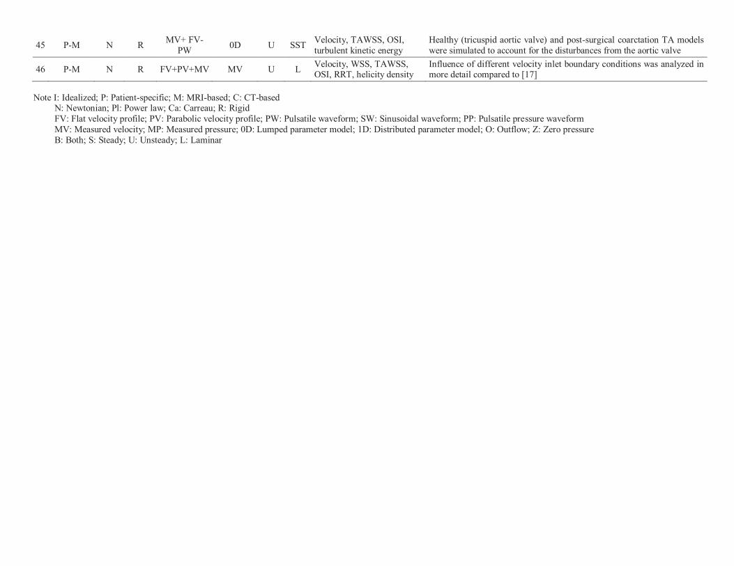
45 P-M N R MV+ FV-

PW 0D U SST

Velocity, TAWSS, OSI,

turbulent kinetic energy

Healthy (tricuspid aortic valve) and post-surgical coarctation TA models

were simulated to account for the disturbances from the aortic valve

46 P-M N R FV+PV+MV MV U L Velocity, WSS, TAWSS, OSI, RRT, helicity density

Influence of different velocity inlet boundary conditions was analyzed in more detail compared to [17]

Note I: Idealized; P: Patient-specific; M: MRI-based; C: CT-based N: Newtonian; Pl: Power law; Ca: Carreau; R: Rigid

FV: Flat velocity profile; PV: Parabolic velocity profile; PW: Pulsatile waveform; SW: Sinusoidal waveform; PP: Pulsatile pressure waveform

MV: Measured velocity; MP: Measured pressure; 0D: Lumped parameter model; 1D: Distributed parameter model; O: Outflow; Z: Zero pressure

B: Both; S: Steady; U: Unsteady; L: Laminar

View publication statsView publication stats