A reversible mesoscopic model of di usion in liquids: from...

A reversible mesoscopic model of diffusion in liquids:from giant fluctuations to Fick’s law

Aleksandar Donev

Courant Institute, New York University&

Eric Vanden-Eijnden, Courant

Polymer Physics SeminarETH, Zurich

May 22nd 2014

A. Donev (CIMS) Diffusion 5/2014 1 / 34

Giant Fluctuations

Diffusion in Liquids

There is a common belief that diffusion in all sorts of materials,including gases, liquids and solids, is described by random walks andFick’s law for the concentration of labeled (tracer) particles c (r, t),

∂tc = ∇ · [χ (r)∇c] ,

where χ � 0 is a diffusion tensor.But there is well-known hints that the microscopic origin of Fickiandiffusion is different in liquids from that in gases or solids, and thatthermal velocity fluctuations play a key role.The Stokes-Einstein relation connects mass diffusion tomomentum diffusion (viscosity η),

χ ≈ kBT

6πση,

where σ is a molecular diameter.Macroscopic diffusive fluxes in liquids are known to be accompaniedby long-ranged nonequilibrium giant concentration fluctuations [1].


Giant Fluctuations

Giant Nonequilibrium Fluctuations

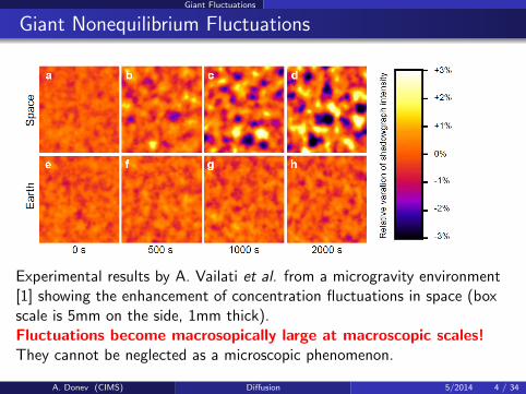
Experimental results by A. Vailati et al. from a microgravity environment[1] showing the enhancement of concentration fluctuations in space (boxscale is 5mm on the side, 1mm thick).Fluctuations become macrosopically large at macroscopic scales!They cannot be neglected as a microscopic phenomenon.


Giant Fluctuations

Hydrodynamic Correlations

The mesoscopic model we develop here applies, to a certain degree ofaccuracy, to two seemingly very different situations:

1 Molecular diffusion in binary fluid mixtures, notably, diffusion of taggedparticles (e.g., fluorescently-labeled molecules in a FRAP experiment).

2 Diffusion of colloidal particles at low concentrations.

The microscopic mechanism of molecular diffusion in liquids isdifferent from that in either gases or solids due to the effects ofcaging:

1 The Schmidt number is very large (unlike gases) and particlesremain trapped in their cage while fast molecular collisions(interactions) diffuse momentum and energy.

2 The breaking and movement of cages requires collective(hydrodynamic) rearrangement and thus the assumption ofindependent Brownian walkers is not appropriate.This is well-appreciated in the colloidal literature and is described ashydrodynamic “interactions” (really, hydrodynamic correlations), butwe will see that the same applies to molecular diffusion.


Brownian Dynamics Model

Brownian Dynamics

The Ito equations of Brownian Dynamics (BD) for the (correlated)positions of the N particles Q (t) = {q1 (t) , . . . ,qN (t)} are

dQ = −M (∂QU) dt + (2kBT M)12 dB + kBT (∂Q ·M) dt, (1)

where B(t) is a collection of independent Brownian motions, U (Q) isa conservative interaction potential.

Here M (Q) � 0 is a symmetric positive semidefinite mobility blockmatrix for the collection of particles, and introduces correlationsamong the walkers.

The Fokker-Planck equation (FPE) for the probability density P (Q, t)corresponding to (1) is

∂P

∂t=

∂

∂Q·{

M

[∂U

∂QP + (kBT )

∂P

∂Q

]}, (2)

and is in detailed-balance (i.e., is time reversible) with respect to theGibbs-Boltzmann distribution ∼ exp (−U(Q)/kBT ).



Hydrodynamic Correlations

Let’s start from the (low-density) pairwise approximation

∀ (i , j) : Mij

(qi ,qj

)=

R(qi ,qj

)kBT

=1

kBT

∑k

φk (qi )φk

(qj

),

Here R (r, r′) is a symmetric positive-definite kernel that isdivergence-free, and can be diagonalized in an (infinite dimensional)set of divergence-free basis functions φk (r).

For the Rotne-Prager-Yamakawa tensor mobility,R(r′, r′′) ≡R(r′ − r′′ ≡ r),

R(r) = χ

(

3σ

4r+σ3

2r3

)I +

(3σ

4r− 3σ3

2r3

)r ⊗ r

r2, r > 2σ(

1− 9r

32σ

)I +

(3r

32σ

)r ⊗ r

r2, r ≤ 2σ

(3)

where σ is the radius of the colloidal particles and the diffusioncoefficient χ follows the Stokes-Einstein formula χ = kBT/ (6πησ).



Lagrangian Overdamped Dynamics

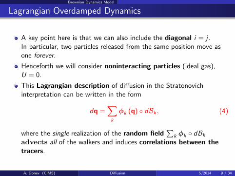
A key point here is that we can also include the diagonal i = j .In particular, two particles released from the same position move asone forever.

Henceforth we will consider noninteracting particles (ideal gas),U = 0.

This Lagrangian description of diffusion in the Stratonovichinterpretation can be written in the form

dq =∑k

φk (q) ◦ dBk , (4)

where the single realization of the random field∑

k φk ◦ dBkadvects all of the walkers and induces correlations between thetracers.



Eulerian Overdamped Dynamics

We can use standard calculus to obtain an equation for the empiricalor instantaneous concentration

c (r, t) =N∑i=1

δ (qi (t)− r) . (5)

We will write the result shortly, after we derive it from a fluctuatinghydrodynamics perspective:derivation relies closely on divergence-free condition [2].

Aside: For uncorrelated walkers, Mij = δij (kBT )−1 χI, one canformally write the (ill-defined) Ito stochastic partial differentialequation (SPDE) [3],

∂tc = χ∇2c + ∇ ·(√

2χcWc

), (6)

where Wc (r, t) denotes a spatio-temporal white-noise vector field.


Fluctuating Hydrodynamics Model

Fluctuating Hydrodynamics

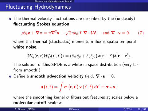
The thermal velocity fluctuations are described by the (unsteady)fluctuating Stokes equation,

ρ∂tv + ∇π = η∇2v +√

2ηkBT ∇ ·W , and ∇ · v = 0. (7)

where the thermal (stochastic) momentum flux is spatio-temporalwhite noise,

〈Wij(r, t)W?kl(r′, t ′)〉 = (δikδjl + δilδjk) δ(t − t ′)δ(r − r′).

The solution of this SPDE is a white-in-space distribution (very farfrom smooth!).

Define a smooth advection velocity field, ∇ · u = 0,

u (r, t) =

∫σ(r, r′)

v(r′, t)dr′ ≡ σ ? v,

where the smoothing kernel σ filters out features at scales below amolecular cutoff scale σ.



Resolved (Full) Dynamics

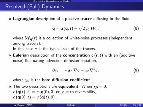
Lagrangian description of a passive tracer diffusing in the fluid,

q̇ = u (q, t) +√

2χ0 Wq, (8)

where Wq(t) is a collection of white-noise processes (independentamong tracers).In this case σ is the typical size of the tracers.

Eulerian description of the concentration c (r, t) with an (additivenoise) fluctuating advection-diffusion equation,

∂tc = −u ·∇c + χ0∇2c, (9)

where χ0 is the bare diffusion coefficient.

The two descriptions are equivalent. When χ0 = 0,c (q(t), t) = c (q(0), 0) or, due to reversibility,c (q(0), t) = c (q(t), 0).



Fractal Fronts in Diffusive Mixing

Snapshots of concentration in a miscible mixture showing the developmentof a rough diffusive interface due to the effect of thermal fluctuations[4]. These giant fluctuations have been studied experimentally [1] andwith hard-disk molecular dynamics [5].Our Goal: Computational modeling of diffusive mixing in liquids inthe presence of thermal fluctuations.


Overdamped Limit

Separation of Time Scales

In liquids molecules are caged (trapped) for long periods of time asthey collide with neighbors:Momentum and heat diffuse much faster than does mass.

This means that χ� ν, leading to a Schmidt number

Sc =ν

χ∼ 103 − 104.

This extreme stiffness solving the concentration/tracer equationnumerically challenging.

There exists a limiting (overdamped) dynamics for c in the limitSc →∞ in the scaling [6]

χν = const.


Overdamped Limit

Eulerian Overdamped Dynamics

Adiabatic mode elimination gives the following limiting stochasticadvection-diffusion equation (reminiscent of the Kraichnan’s modelin turbulence),

∂tc = −w �∇c + χ0∇2c, (10)

where � denotes a Stratonovich dot product.

The advection velocity w (r, t) is white in time, with covarianceproportional to a Green-Kubo integral of the velocity auto-correlationfunction,

〈w (r, t)⊗w(r′, t ′

)〉 = 2 δ

(t − t ′

) ∫ ∞0〈u (r, t)⊗ u

(r′, t + t ′

)〉dt ′,

In the Ito interpretation, there is enhanced diffusion,

∂tc = −w ·∇c + χ0∇2c + ∇ · [χ (r)∇c] (11)

where χ (r) is an analog of eddy diffusivity in turbulence.


Overdamped Limit

Diffusion Coefficient

Let us factorize the integral of the velocity correlation function insome (infinite dimensional) set of basis functions φk (r),∫ ∞

0〈u (r, t)⊗ u

(r′, t + t ′

)〉dt ′ =

∑k

φk (r)⊗ φk

(r′).

For periodic boundaries φk can be Fourier modes but in general theydepend on the boundary conditions for the velocity.

The notation w �∇c is a short-hand for∑

k (φk ·∇c) ◦ dBk/dt,where Bk (t) are independent Brownian motions (Wiener processes).

Similarly, w ·∇c is shorthand notation for∑

k (φk ·∇c) dBk/dt.

The enhanced or fluctuation-induced diffusion is

χ (r) =

∫ ∞0〈u (r, t)⊗u

(r, t + t ′

)〉dt ′ =

∑k

φk (r)⊗φk (r) = R (r, r) .


Overdamped Limit

Back to Lagrangian description

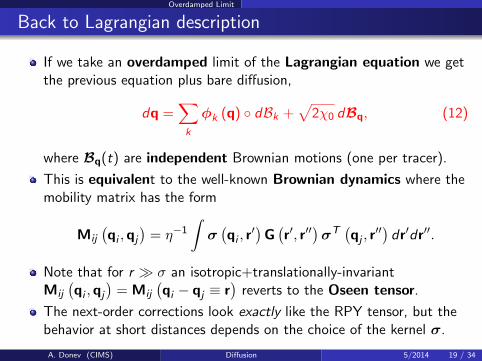
If we take an overdamped limit of the Lagrangian equation we getthe previous equation plus bare diffusion,

dq =∑k

φk (q) ◦ dBk +√

2χ0 dBq, (12)

where Bq(t) are independent Brownian motions (one per tracer).

This is equivalent to the well-known Brownian dynamics where themobility matrix has the form

Mij

(qi ,qj

)= η−1

∫σ(qi , r

′)G(r′, r′′

)σT(qj , r

′′) dr′dr′′.

Note that for r � σ an isotropic+translationally-invariantMij

(qi ,qj

)= Mij

(qi − qj ≡ r

)reverts to the Oseen tensor.

The next-order corrections look exactly like the RPY tensor, but thebehavior at short distances depends on the choice of the kernel σ.


Overdamped Limit

Stokes-Einstein Relation

An explicit calculation for Stokes flow gives the explicit result

χ (r) =kBT

η

∫σ(r, r′)

G(r′, r′′

)σT(r, r′′

)dr′dr′′, (13)

where G is the Green’s function for steady Stokes flow.For an appropriate filter σ, this gives Stokes-Einstein formula forthe diffusion coefficient in a finite domain of length L,

χ =kBT

η

{(4π)−1 ln L

σ if d = 2

(6πσ)−1(

1−√

22σL

)if d = 3.

The limiting dynamics is a good approximation if the effectiveSchmidt number Sc = ν/χeff = ν/ (χ0 + χ)� 1.The fact that for many liquids Stokes-Einstein holds as a goodapproximation implies that χ0 � χ:Diffusion in liquids is dominated by advection by thermalvelocity fluctuations, and is more similar to eddy diffusion inturbulence than to standard Fickian diffusion.


Numerics

Multiscale Numerical Algorithm

The limiting dynamics can be efficiently simulated using the followingpredictor-corrector algorithm (implemented on GPUs):

1 Generate a random advection velocity by solving steady Stokes withrandom forcing,

∇πn+ 12 = ν

(∇2vn

)+ ∆t−

12∇ ·

(√2νρ−1 kBT Wn

)∇ · vn = 0.

using a staggered finite-volume fluctuating hydrodynamics solver [4],and compute un = σ ? vn by filtering.

2 Do a predictor advection-diffusion solve for concentration,

c̃n+1 − cn

∆t= −un ·∇cn + χ0∇2

(cn + c̃n+1

2

).

3 Take a corrector step for concentration,

cn+1 − cn

∆t= −un ·∇

(cn + c̃n+1

2

)+ χ0∇2

(cn + cn+1

2

).


Numerics

Lagrangian Algorithm

The tracer Lagrangian dynamics can be efficiently simulated withoutartificial dissipation (implemented on GPUs):

1 Generate a random advection velocity by solving steady Stokes withrandom forcing

∇πn+ 12 = ν

(∇2vn

)+ ∆t−

12∇ ·

(√2νρ−1 kBT Wn

)∇ · vn = 0.

using a spectral (FFT-based) algorithm.2 Filter the velocity with a Gaussian filter (in Fourier space),

wn = σ ? vn.

3 Use a non-uniform FFT to evaluate un = wn(qn), and move thetracers,

qn+1 = q + un∆t.

In non-periodic domains one would need to do a corrector step for tracers(Euler-Heun method for the Stratonovich SDE).


Numerics

Numerical Issues

1 All algorithms implemented on GPUs for periodic boundaries usingFFTs. We do large simulations in 2D here to study physics, 3D isimplemented but largest grid is O(5123).

2 Eulerian algorithm also implemented in IBAMR library by BoyceGriffith, to be used for studying the effect of boundary conditions inexperiments on giant fluctuations.

3 For Eulerian algorithm the difficulty is in the advection: we needessentially non-dissipative advection that is also good withmonotonicity preserving.

4 Right now we use a strictly non-dissipative centered advection, forwhich we can calculate discrete diffusion enhancement operatorexactly.

5 Also trying more sophisticated minimally-dissipative semi-Lagrangianadvection schemes of John Bell implemented by Sandra May(unfinished).


The Physics of Diffusion

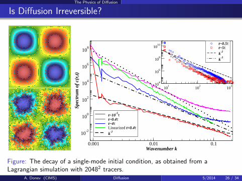
Is Diffusion Irreversible?

0.001 0.01 0.1Wavenumber k

10-2

100

102

104

106

108

Spec

trum

of

c(r,

t)

t~10-5τ

t~0.4τt~4τLinearized t=0.4τk

-2

101

102

10310

4

106

108

1010 t~0.5τ

t~5τk

-2

k-3

Figure: The decay of a single-mode initial condition, as obtained from aLagrangian simulation with 20482 tracers.



Effective Dissipation

The ensemble mean of concentration follows Fick’s deterministiclaw,

∂t〈c〉 = ∇ · (χeff∇〈c〉) = ∇ · [(χ0 + χ)∇〈c〉] , (14)

which is well-known from stochastic homogenization theory.

The physical behavior of diffusion by thermal velocity fluctuations isvery different from classical Fickian diffusion:Standard diffusion (χ0) is irreversible and dissipative, butdiffusion by advection (χ) is reversible and conservative.

Spectral power is not decaying as in simple diffusion but is transferredto smaller scales, like in the turbulent energy cascade.

This transfer of power is effectively irreversible because power“disappears”. Can we make this more precise?



Virtual FREP Experiment (χ0 = 0)

The contour lines become very rough, and eventually fill the whole plane,unless we put some bare diffusion to smooth things out.But this generates sub-molecular scale features, compare to hard-diskmolecular dynamics (1M disks):

We should perform spatial coarse-graining to study cδ = δ ? c, whereδ > σ is a mesoscopic measurement (observation) scale.



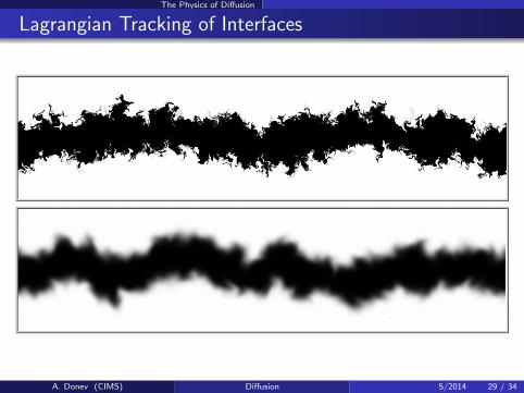
Lagrangian Tracking of Interfaces



Spatial Coarse-Graining

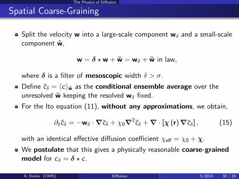
Split the velocity w into a large-scale component wδ and a small-scalecomponent w̃,

w = δ ?w + w̃ = wδ + w̃ in law,

where δ is a filter of mesoscopic width δ > σ.

Define c̄δ = 〈c〉w̃ as the conditional ensemble average over theunresolved w̃ keeping the resolved wδ fixed.

For the Ito equation (11), without any approximations, we obtain,

∂t c̄δ = −wδ ·∇c̄δ + χ0∇2c̄δ + ∇ · [χ (r)∇c̄δ] , (15)

with an identical effective diffusion coefficient χeff = χ0 + χ.

We postulate that this gives a physically reasonable coarse-grainedmodel for cδ = δ ? c.



Coarse-Grained Equations

In the Stratonovich interpretation the coarse-grained equation is

∂tcδ ≈ −wδ �∇cδ + ∇ · [(χ0 + ∆χδ)∇cδ] , (16)

where the diffusion renormalization ∆χδ (r) [7, 8] is

∆χδ = χ− δ ? χ ? δT . (17)

The coarse-grained equation has true dissipation (irreversibility)since ∆χδ > 0.

For δ � σ in three dimensions we get ∆χδ ≈ χ and so thecoarse-grained equation becomes Fick’s law with Stokes-Einstein’sform for the diffusion coefficient. This hints thatIn three dimensions (but not in two dimensions!) atmacroscopic scales Fick’s law applies. At mesoscopic scalesfluctuating hydrodynamics with renormalized transportcoefficients is a good model.



Irreversible vs. Reversible Dynamics

Figure: (Top panel) Diffusive mixing studied using the Lagrangian traceralgorithm. (Bottom) The spatially-coarse grained concentration cδ obtained byblurring with a Gaussian filter of two different widths.



Conclusions

Fluctuations are not just a microscopic phenomenon: giantfluctuations can reach macroscopic dimensions or certainly dimensionsmuch larger than molecular.

Fluctuating hydrodynamics describes these effects.

Due to large separation of time scales between mass andmomentum diffusion we need to find the limiting dynamics toeliminate the stiffness.

The overdamped equation is a stochastic advection-diffusionequation with a white-in-time velocity.

Diffusion in liquids is strongly affected and in fact dominated byadvection by velocity fluctuations.

This kind of “eddy” diffusion is very different from Fickian diffusion: itis reversible (conservative) rather than irreversible (dissipative)!

At macroscopic scales, however, one expects to recover Fick’sdeterministic law, in three, but not in two dimensions.



References

A. Vailati, R. Cerbino, S. Mazzoni, C. J. Takacs, D. S. Cannell, and M. Giglio.

Fractal fronts of diffusion in microgravity.Nature Communications, 2:290, 2011.

A. Donev and E. Vanden-Eijnden.

Dynamic Density Functional Theory with hydrodynamic interactions and fluctuations.Submitted to J. Chem. Phys., Arxiv preprint 1403.3959, 2014.

David S Dean.

Langevin equation for the density of a system of interacting langevin processes.Journal of Physics A: Mathematical and General, 29(24):L613, 1996.

F. Balboa Usabiaga, J. B. Bell, R. Delgado-Buscalioni, A. Donev, T. G. Fai, B. E. Griffith, and C. S. Peskin.

Staggered Schemes for Fluctuating Hydrodynamics.SIAM J. Multiscale Modeling and Simulation, 10(4):1369–1408, 2012.

A. Donev, A. J. Nonaka, Y. Sun, T. G. Fai, A. L. Garcia, and J. B. Bell.

Low Mach Number Fluctuating Hydrodynamics of Diffusively Mixing Fluids.Communications in Applied Mathematics and Computational Science, 9(1):47–105, 2014.

A. Donev, T. G. Fai, and E. Vanden-Eijnden.

Reversible Diffusion by Thermal Fluctuations.Arxiv preprint 1306.3158, 2013.

D. Bedeaux and P. Mazur.

Renormalization of the diffusion coefficient in a fluctuating fluid I.Physica, 73:431–458, 1974.

A. Donev, T. G. Fai, and E. Vanden-Eijnden.

A reversible mesoscopic model of diffusion in liquids: from giant fluctuations to fick’s law.Journal of Statistical Mechanics: Theory and Experiment, 2014(4):P04004, 2014.


A reversible mesoscopic model of di usion in liquids: from...

Documents

Transcript of A reversible mesoscopic model of di usion in liquids: from...