arX

iv:2

010.

0770

8v1

[cs

.RO

] 1

5 O

ct 2

020

A Reversible Dynamic Movement Primitive

formulation

Antonis SidiropoulosAutomation & Robotics Lab

Dept. of Electrical & Computer EngineeringAristotle University of Thessaloniki, Greece

antosidi@ece.auth.gr

Zoe DoulgeriAutomation & Robotics Lab

Dept. of Electrical & Computer EngineeringAristotle University of Thessaloniki, Greece

doulgeri@eng.auth.gr

Abstract: In this work, a novel Dynamic Movement Primitive (DMP) formulationis proposed which supports reversibility, i.e. backwards reproduction of a learnedtrajectory, while also sharing all favourable properties of classical DMP. ClassicalDMP have been extensively used for encoding and reproducing a desired motionpattern in several robotic applications. However, they lack reversibility, which isa useful and expedient property that can be leveraged in many scenarios. The pro-posed formulation is analyzed theoretically and is validated through simulationsand experiments.

Keywords: Dynamic Movement Primitives, Reversibility, Programming byDemonstration

1 Introduction

The technological advancements in the field of robotics over the past few years have triggered a surgein research interest for incorporating robots more and more actively in everyday life. Robots are al-ready employed widely in industry and their use in household environments is envisaged vividly.Still, programming a robot to perform even simple tasks usually requires considerable amount oftime and advanced robotic and programming knowledge. To facilitate this cause, the use of Pro-gramming by Demonstration (PbD) has been proposed for passing on human skills to a robot [1].At the core of this approach is a model used for encoding the demonstrated trajectory encapsulatingthe desired motion pattern for performing a task. The properties of this model play a major role, asthey determine whether the encoded motion is amenable to generalization, online adaption, reverseexecution etc, depending on the target application.

In the literature there are a lot of approaches for encoding a desired motion pattern, such as splinedecomposition [2], neural networks [3], Hidden Markov Models [4], Gaussian Process Regression[5], Gaussian Mixture Models [6] and more. Undoubtedly, one of the most prominent approachesis the Dynamic Movement Primitives which have been applied in numerous robotic applications[7, 8, 9, 10, 11]. The reason behind this widespread applicability of DMP is mainly attributed to thefavourable properties they come along with. Specifically, they offer a fairly simple framework forencoding any smooth non-linear trajectory, allowing generalization to new targets (end points) andchanging the speed of execution. Moreover, they guarantee global asymptotic stability (GAS) at thetarget, robustness to target perturbations and allow seamlessly the encoding and synchronization ofmultiple DoFs. All these properties make DMP quite the appealing and efficient choice to opt forwhen encoding a desired motion pattern. However, there is still room and need for improvement.There are many tasks where reversibility, i.e. reproduction of the learned trajectory backwards intime, could come quite in handy.

For many tasks, reverse execution could enable automatic derivation of certain required operationsfrom their forwards counterparts. For instance, in assembly tasks a reversible model could be usedfor assembling and disassembling a workpiece. More generally, when performing any task thatinvolves reaching, like a handover, a placing or an insertion task etc, the reverse motion could beused for the retraction, saving the effort of explicitly encoding and programming the backwardmotion. This becomes even more useful in tasks executed in cluttered environments. Reversibility

4th Conference on Robot Learning (CoRL 2020), Cambridge MA, USA.

can also prove really effective and practical for recovering from errors during the execution of atask. These errors could originate from faulty or noisy sensor measurements or could be attributed todisturbances. Using reverse execution, the robot can temporarily back out of an erroneous situationby tracing back to a previous point, after which the execution can be automatically retried. Thereare some works that have applied reversibility to recover from such errors in practical applications[12, 13]. In these works, the authors address error recovery by reversing the program’s executionby means of designing a domain specific language (DSL) which supports running backwards theexecuted programming commands. A more theoretical treatment of reversibility using DMP is givenin [14]. As classical DMP do not support reversibility, the authors in [14] come forward with amodified DMP structure in order to attain reversibility. However, due to the adopted formulation,global asymptotic stability (GAS) and reversibility cannot be achieved simultaneously. Eventuallythe authors resort to the use of two separate DMPs to ensure both.

In this work, we propose a novel DMP formulation that achieves reversibility, maintaining also allthe favourable properties of classical DMP, such as spatial and temporal scaling, GAS, robustness totarget perturbations and on-line adaptation via the addition of coupling terms. The novel formulationcomes along with some additional properties. Specifically, training requires only position measure-ments and is decoupled from the DMP’s stiffness and damping gains. Additionally, the DMP’seffective stiffness and damping is not dependent on the temporal scaling parameter, as opposed toclassical DMP. Moreover, the proposed DMP allows a two phase PbD scheme that is particularlysuitable for encoding tasks that require high precision during the demonstration of the desired path.The proposed DMP is compared with the classical in various simulations and is further validatedthrough experiments.

The rest of this paper is organized as follows: section 2 provides an overview on classical DMP.In section 3 the proposed DMP formulation is presented and its properties are compared with theclassical one in section 4 via simulations. Experimental results are presented in section 5 and con-clusions are drawn in section 6. In the appendix, the correspondence between the proposed andclassical DMP formulations is theoretically analyzed.

2 Dynamic Movement Primitives Preliminaries

DMP consist of a transformation system which generates a trajectory and a canonical system forcontrolling the system’s temporal evolution [15]. The transformation system is composed of twoterms, a second order linear attractor to a goal and a non-linear forcing term which has to be learnedin order to encode a desired kinematic behavior. Aggregating the different variants that have beenproposed in the literature in a more generic formulation a 1-DoF DMP is given as follows:

τ2y = αzβz(g − y)− αzτ y + gf (x)(g − y0)fs(x) (1)

τx = h(x) (2)

or expressing (1) in state equations introducing z = τ y:

τ z = αzβz(g − y)− αzz + gf (x)(g − y0)fs(x) (3)

τ y = z (4)

where y, y is the position and velocity, g the target, y0 the initial position. The phase variable x isused to avoid direct dependency on time and τ > 0 is a temporal scaling parameter, typically setequal to the movement’s total duration T = tf − t0, where t0 is the initial and tf the final timeinstant. The forcing term fs(x) is given by:

fs(x) = φ(x)Tw (5)

where φ(x)T = [ψ1(x) · · · ψN (x)]/∑N

i=1 ψi(x), with ψi(x) = exp(−hi(x − ci)2). The gating

function gf (x) ensures that the forcing term eventually vanishes thus (1) acts as a spring-damperand converges asymptotically to the goal g.

The canonical system’s evolution is determined by (2), with h(x) chosen so that x evolves monoton-ically from its initial value x(0) = x0 to its final value x(tf ) = xf . Many options are available, e.g.τx = 1 with x0 = 0 and xf = 1 or τx = −axx with x0 = 1 and xf = 0+. For the gating functiongf (x) there are many choices as well, such as linear, exponential or sigmoid gating, to name but afew. Regarding the choice of αz, βz a typical approach is to set βz = αz/4 > 0 to render the linear

2

part of (1) critically damped. To achieve good approximation during learning, a general heuristic isto place the centers ci of the Gaussian kernels in (5) equally spaced in time. A typical choice is tothen set the inverse widths of the Gaussians as hi =

ah

(ci+1−ci)2, hN = hN−1, i = 1, · · · , N , where

ah > 0 is a scaling factor controlling the overlapping between the kernels.

3 A Reversible Dynamic Movement Primitive

Reversibility of DMP means that the generated system’s trajectory will be identical in forward andbackward motion. Given a goal attractor dynamics e.g. (1), it is however impossible to have globalstability and reversibility simultaneously as also noted in [14]. In Appendix B we also provide aproof that the classical DMP are indeed not reversible. In order to produce a reversible DMP theauthors in [14] suggest a non-linear system with two equilibria, an attractor and a repeller, and buildtheir proposed formulation around it. This formulation achieves partial reversibility if the solutionstays within a region and becomes unstable beyond. As the solution cannot be guaranteed to staywithin the permitted region, which is expected as the basic dynamics are non-linear, the authorsfinally resort to using two forcing terms to ensure global stability. Instead of having a goal attractoras a foundation of the transformation system we base our novel formulation on a linear system witha global asymptotically stable origin. Inspired by linear trajectory tracking dynamics we proposethe following DMP structure for 1-DoF :

y = yx −D(y − yx)−K(y − yx) (6)

x = h(x)/τ , x(t0/τ) = x0 , x(tf/τ) = xf (7)

where K,D are positive scalars, h(x) satisfies h(x) = 0 for x outside of the interval defined by x0and xf , with its time integral being a strictly monotonically evolving function w.r.t. time and yx isthe desired spatially and temporally scaled trajectory that is generated by:

yx , ks(fp(x)− fp(x0)) + y0 (8)

yx(t) = ksfp(x) (9)

yx(t) = ksfp(x) (10)

where

ks ,g − y0

fp(xf )− fp(x0)(11)

is the spatial scaling term and

fp(x) = φ(x)Tw (12)

encodes the demonstrated position yd through a weighted sum of Gaussians. Learning of the weightsw can be performed using Locally Weighted Regression (LWR), Least Squares (LS) or any other

optimization technique. The derivatives of fp(x) can be calculated from fp(x) = (∂φ∂x x)Tw and

fp(x) = (∂2φ

∂x2 x2 + ∂φ

∂x x)Tw.

Forward reproduction of the learned trajectory is accomplished integrating (6)-(7). For backwardreproduction only the sign of x needs to be flipped, i.e. x = −h(x)/τ , x(t0/τ) = xf .

Denoting e = y − yx and considering that D,K > 0 it follows from (6) that e, e, e → 0. What ismore, as yx and its derivatives are bounded by construction, y, y, y are bounded as well. In forwardreproduction (7) implies that x → xf and x, x → 0, and from (8)-(10) and (11) we can concludethat yx → g, yx, yx → 0. Therefore, y → g, y, y → 0. In backward reproduction from any x 6= x0,x = −h(x)/τ implies x → x0 and x, x → 0 therefore from (8)-(10) and (11) we get that yx → y0,yx, yx → 0, hence y → y0, y, y → 0.

For Cartesian position encoding the above formulation is readily extended as each DoF can beencoded separately and synchronization can be achieved using the same canonical system (7) for allDoFs. Regarding Cartesian orientation, a formulation analogous to (6) is adopted, which makes useof the quaternion logarithm as in [16] (a brief summary on unit quaternions is provided in Appendix

C). Introducingη , log(Q∗Q0), where Q is the current, Q0 the initial orientation expressed as unit

quaternions, ∗ denotes the quaternion product, (.) the quaternion inverse and log(.) the quaternionlogarithm, the novel DMP formulation for Cartesian orientation is given by:

η = ηx −D(η − ηx)−K(η − ηx) (13)

3

with the canonical system given by (7). The matrices K, D are diagonal positive definite stiffnessand damping matrices. The desired spatially and temporally scaled trajectory is given by:

ηx , Ksfq(x) (14)

where Ks , diag (ηg./fq(xf )) with ηg , log(Qg ∗ Q0), Qg is the target orientation and ./denotes the element-wise division. The desired motion is learned based only on the demonstratedorientation ηd = log(Qd ∗ Qd,0), where Qd and Qd,0 are the demonstrated and initial orientation,through fq(x) which is a weighted sum of Gaussians:

fq(x) = Wφ(x) (15)

where W = [wx wy wz]T , with wi being the weights for each coordinate i ∈ x, y, z. The

desired scaled velocity ηx and acceleration ηx are obtained by differentiating ηx(t) as in (9), (10).The orientation Q, rotational velocity ω and acceleration ω can be obtained from η, η, η usingQ = exp(η)∗Q0 and (37), (38) from Appendix C. Finally, the stabilty analysis for 1-DoF is readilyextended to the orientation formulation (13), as each DoF in η is decoupled.

4 Properties and Comparison with classical DMP

As mentioned in the introduction, DMP have a number of desirable properties. Hence any alternativeformulation should also have these properties to remain an appealing choice when encoding a de-sired pattern. In this section we show and demonstrate by comparative simulations that the proposedreversible DMP retains these properties. We further discuss additional benefits apart from reversibil-ity that come with the proposed formulation. Simulations also include the trajectories generated byreverse execution.

4.1 Standard DMP properties

Guaranteed convergence to the goal has already been discussed for the proposed DMP in the pre-vious section. It is also clear that the stable coordination of multiple DoF is similar to the classicalDMP, using a common canonical system for all DoFs. Moreover, the forcing term is linear withrespect to the weights as in the classical DMP.

Spatial and temporal scaling:

The spatial and temporal scaling property pertains to the system being able to generate trajectoriesthat are qualitatively similar or topologically equivalent [15] when there is a change in the initial po-sition, goal, or temporal scaling parameter. More details regarding scaling are provided in AppendixA.

For the comparative simulation, we trained both the classical and the proposed DMP using as train-ing data a fifth order polynomial with initial position yd,0 = 0, target gd = 1 and duration T = 2sec. Training is performed using Least Squares. For both DMP we use 30 kernels, with centersand widths placed as described in section 2 and we set τ = T . A linear canonical system is usedwith x0 = 0 and xf = 1. For the classical DMP, an exponential gating function is used, i.e.

gf (x) = e−4.6x, which ensures that gf (xf ) ≈ 0.01. To examine spatial scaling, both DMPs aresimulated for new targets that correspond to spatial scalings ks ∈ −2,−1.5,−0.5, 0.5, 1.5, 2. Fortemporal scaling we choose τ so that kt = τd/τ ∈ 0.5, 0.7, 0.85, 1.3, 1.6. The proposed DMPis also simulated in reverse with the same scalings. Results are presented in Fig. 1-2, where it canbe observed that the proposed DMP coincides with the classical one in forward motions, while thereverse trajectory is the mirrored (w.r.t time) of the respective forward trajectory, as expected.

Time modulation:

This property refers to the ability of speeding up or slowing down the trajectory generation and evenbringing it to an halt by modifying the canonical system’s evolution. The latter is achieved with theso called phase stopping, and is applied in the presence of an external disturbance based on the errorbetween the DMP’s output y and the actual position of a robot or an external force measurement etc.The proposed DMP retains this property and phase stopping is formulated in a way analogous to theclassical DMP. The modification of the canonical system’s evolution is given by:

τx =h(x)

1 + ad|d(t)|(16)

4

0 1 2 3 40

0.2

0.4

0.6

0.8

1

Figure 1: Temporal scaling of classical andnovel DMP for kt ∈ 0.5, 0.7, 0.85, 1.3, 1.6.

0 0.5 1 1.5 2-2

-1

0

1

2

Figure 2: Spatial scaling of classical and novelDMP for ks ∈ −2,−1.5,−0.5, 0.5, 1.5, 2.

where ad > 0 and d(t) is the applied disturbance. For the classical DMP, halting the evolution of xdoes not suffice as the goal attractor αzβz(g−y) in (1) would make y to continue evolving. Instead,the temporal scaling τ must be adjusted accordingly:

τ ′ = τ(1 + ad|d(t)|) (17)

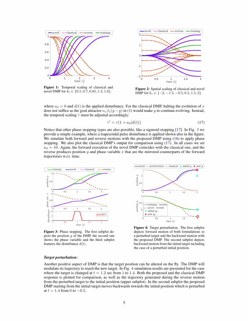
Notice that other phase stopping types are also possible, like a sigmoid stopping [17]. In Fig. 3 weprovide a simple example, where a trapezoidal pulse disturbance is applied shown also in the figure.We simulate both forward and reverse motions with the proposed DMP using (16) to apply phasestopping. We also plot the classical DMP’s output for comparison using (17). In all cases we setad = 10. Again, the forward execution of the novel DMP coincides with the classical one, and thereverse produces position y and phase variable x that are the mirrored counterparts of the forwardtrajectories w.r.t. time.

0 0.5 1 1.5 20

0.5

1

0 0.5 1 1.5 20

0.5

1

0 0.5 1 1.5 20

5

10

Figure 3: Phase stopping. The first subplot de-picts the position y of the DMP, the second oneshows the phase variable and the third subplotfeatures the disturbance d(t).

0 0.5 1 1.5 20

0.5

1

0 0.5 1 1.5 2

0

0.5

1

Figure 4: Target perturbation. The first subplotdepicts forward motion of both formulations toa perturbed target and the backward motion withthe proposed DMP. The second subplot depictsbackward motion from the initial target includingthe case of a perturbed initial position.

Target perturbation:

Another positive aspect of DMP is that the target position can be altered on the fly. The DMP willmodulate its trajectory to reach the new target. In Fig. 4 simulation results are presented for the casewhere the target is changed at t = 1.2 sec from 1 to 1.4. Both the proposed and the classical DMPresponse is plotted for comparison, as well as the trajectory generated during the reverse motionfrom the perturbed target to the initial position (upper subplot). In the second subplot the proposedDMP starting from the initial target moves backwards towards the initial position which is perturbedat t = 1.4 from 0 to −0.5.

5

Notice in the first subplot, the slower response of the classical DMP which is attributed to the factthat the effective stiffness and damping in the classical DMP are dependent on τ (see equation (26)in Appendix A). Thus, for τ > 1 the stiffness and damping will decrease, leading to a slowerresponse and vice versa. In contrast, in the proposed DMP, the stiffness and damping values aredecoupled from τ (6), which is an additional merit provided by this formulation. Clearly, for τ = 1,the responses of both formulations would be identical.

Incorporation of coupling terms:

DMP allow online modifications of the dynamical system’s trajectory based on external signals,referred to as coupling terms. Coupling terms have been applied to adjust online the DMP’s trajec-tory based on the external force measurements [7], to enforce position/joint limits [18], for obstacleavoidance [19] and other. Here we examine the case of enforcing position limits and obstacle avoid-ance. For both cases we use a 2D trajectory obtained by kinesthetically guiding a Kuka lwr4+ robotand recording its end-effector position. For limits avoidance we modify the DMP’s velocity with arepulsive force at the limit [18]:

τ y = z −γ

(yL − y)3(18)

where yL is the limit and γ > 0 controls the effect of the repulsive force. In our simulation we setyL = [∞ 0.72]T and γ = 1e−6. For the classical DMP simulation we use (3) and (18). Introducingthe state z = y, the novel DMP can also be written in the form of state equations, where we also addthe repulsive force at the velocity level as in the classical DMP:

y = z −γ

(yL − y)3

z = yx −D(z − yx)−K(y − yx)

In both cases a linear canonical system from x0 = 0 to xf = 1 is used. The results are presented inFig. 5. The discrepancy in the response of the two DMPs is due to the fact that in the classical DMPτ affects the DMPs stiffness and damping (see (26)) and scales also the repulsive force. This obser-vation is more general. That is, in the classical DMP, the coupling terms are affected by τ , thereforemaking their effect less clear especially in cases where τ is also time varying. Moreover, the dis-crepancy between the forward and the reverse motion is owning to the coupling term. Couplingterms act like a force (which cannot be reversed like a trajectory) and are used for dynamic changesof the environment. So in the presence of couplings, discrepancies are to be expected. However, ifthe cause of the coupling remains static (like in Fig. 5) this discrepancy will be small.

For obstacle avoidance we insert the coupling proposed in [19]. Denoting by po the obstacle’sposition, the following term is added to the DMP’s acceleration, fo = γRyφe−βφ where γ, β > 0,

R is a rotation around axis k = (po − y) × y by angle π/2 and φ = cos−1( (po−y)T y

|(po−y)||y|). For

our simulations we chose γ = 1000 and β = 8. The results are presented in Fig. 6. Again thediscrepancy between the two DMPs is due to the effect of τ on the classical DMP.

0.1 0.2 0.3 0.4 0.5

0.4

0.45

0.5

0.55

0.6

0.65

0.7

0.75

Figure 5: Limit avoidance using coupling terms.

0.2 0.25 0.3 0.35 0.4 0.45 0.5

0.4

0.45

0.5

0.55

0.6

0.65

0.7

0.75

Figure 6: Obstacle avoidance using couplingterms.

6

4.2 Additional Properties

Apart from reversibility, the proposed formulation decouples the DMP’s stiffness and damping gainsfrom the temporal scaling parameter τ , which can affect the system’s response in the presence ofperturbations or other coupling terms as highlighted in the previous simulations. The learning proce-dure is also decoupled from these gains. Learning requires only position measurements for trainingin contrast to the classical DMP which additionally requires velocity and acceleration measurements.Thus computational effort and memory resource demand are reduced in the proposed formulation.Moreover, since velocity and acceleration measurements are usually noisy, the accuracy of the learn-ing process in the classical approach is affected as opposed to the proposed one. Next we discuss inmore details some additional properties enabled by the structure of the proposed formulation.

Demonstrating a desired trajectory using kinesthetic guidance can prove to be quite cumbersome, asone has to pay attention to guide the robot accurately along the desired path, while at the same timeimposing the desired speed of execution (velocity profile). This places a lot of cognitive load to thedemonstrator and can deteriorate the quality of the demonstration. Moreover, there are tasks whereaccuracy in the demonstrated path is of great essence. As opposed to the classical formulation theproposed reversible DMP allows the following two phase leaning framework to facilitate the humandemonstration:

Phase 1 - path teaching: The demonstrator drives the gravity compensated robot along the desiredpath as slowly as required, so as to not compromise accuracy. The novel DMP is then trained usingthe recorded demonstrated data.

Phase 2 - velocity profile teaching: The robot is under position control, following the output pro-duced by the novel DMP formulation given by (6), driven by the following modified canonicalsystem:

x = −dxx+ sf (fv) , for x < 1

x = x = 0 , for x ≥ 1(19)

with x(0) = 1, x(0) = 0, where dx > 0, fv = nTfext with n = ∂y/∂x|∂y/∂x| being the unit

vector pointing along the direction of the motion, y denotes the Cartesian position and fext

is the external force measured from an F/T sensor mounted at the robot’s wrist. The function

sf (fv) =

fv , for fv ≥ 0

0 , for fv < 0ensures that the motion evolves only forwards along the executed

path. The demonstrator applies forces at the robot’s end-effector. Using (19) ensures that the motioncan only evolve along the path demonstrated in phase 1. The higher the forces along the directionof the motion, the faster will be the evolution of the phase variable x, and so will yx and thereforey as well, leading to the speed up of execution. During this process, the robot’s Cartesian pose isrecorded and when the demonstrator finishes, these recorded data are used to retrain the DMP.

A two phase learning approach was initially presented in [20], where Frenet-Serret frames whereutilized to impose low stiffness along the direction of motion and higher stiffness in the perpendicu-lar axes to constrain the motion along the desired path. An iterative procedure to also determine thevalue of the phase variable at each control step is involved. However, the latter approach involvesmore computations and has more open parameters that have to be tuned. In contrast, the presentedframework is much simpler, which is to be attributed to the structure of the novel DMP formulation.

A similar modification of the canonical system can also be used for phase stopping and bidirectionaldrivability along the path:

x = −dx(x− xd) + fv (20)

with x(0) = 0 (x(0)=1) for forward (reverse) execution and x(0) = xd(0), where xd =1

τ(1+ad||Fext||)for forward motion and with flipped sign for reverse, which is similar to (16).

5 Experimental Results

In this section we demonstrate through experiments on a Kuka lwr4+ robot the performance ofthe proposed reversible DMP. Learning is carried out following the two phase training proceduredescribed in subsection 4.2. During the experiments, the robot is in position control and moves tothree different target poses using as reference the output of the proposed DMP. The first target is

7

the one used during the demonstration. After each target is reached, the novel DMP is executed inreverse to go back to the initial pose. During the forward and backward motion to the third targeta user interacts physically with the robot applying an external wrench Fext measured by an AtiF/T sensor mounted at the robot’s wrist. We apply the phase stopping mechanism given by (20)setting dx = 50 and ad = 5. Results shown in Fig. 7 and 8 demonstrate how the user stops anddrives the robot back for t = 32 − 35 sec during its forward motion and just stops the robot on itsreturn for t = 45 − 47.5 sec during the reverse motion. The 3D Cartesian position and orientationpaths are also plotted in Fig. 9 and 10. The orientation is visualized using the quaternion logarithmη = log(Q ∗ Q0). It is clear that the motion is constrained on the same path when the user appliedforces stops or back drives the end-effector.

30 35 40 45 50

-0.4

-0.2

0

30 35 40 45 50-0.6-0.4-0.2

0

30 35 40 45 50

0.4

0.6

30 35 40 45 500

5

10

Forward Reverse

Figure 7: Position bi-directional trajectories tothe 3rd target with user interaction.

30 35 40 45 500

1

30 35 40 45 500

1

30 35 40 45 50

-1

-0.5

0

30 35 40 45 500

5

10

Forward Reverse

Figure 8: Orientation bi-directional trajectoriesto the 3rd target with user interaction

Figure 9: Position paths for forward and reverse mo-tion to three different targets.

Figure 10: Orientation paths for forward and reversemotion to three different targets, using η = log(Q ∗Q0)

.

6 Conclusions

In this work, a reversible Dynamic Movement Primitive (DMP) formulation was proposed which en-sures global asymptotic stability of the target in both forward and backward motion. All favourableproperties of the classical DMP formulation are retained while a few additional desirable propertiesare supported. The proposed formulation was validated through simulations and experiments andcompared to the classical formulation. In this work, the focus was placed on encoding point-to-pointmotions, however the proposed formulation can be easily extended for rhythmic motions. Futurework will be directed towards highlighting its reversibility and comparative merits in assembly anddisassembly tasks.

8

References

[1] A. Billard, S. Calinon, R. Dillmann, and S. Schaal. Robot Programming by Demonstration,pages 1371–1394. Springer Berlin Heidelberg, Berlin, Heidelberg, 2008. ISBN 978-3-540-30301-5. doi:10.1007/978-3-540-30301-5 60.

[2] Jung-Hoon Hwang, R. C. Arkin, and Dong-Soo Kwon. Mobile robots at your fingertip: Beziercurve on-line trajectory generation for supervisory control. In Proceedings 2003 IEEE/RSJ In-ternational Conference on Intelligent Robots and Systems (IROS 2003) (Cat. No.03CH37453),volume 2, pages 1444–1449 vol.2, 2003.

[3] D. Nicolis, A. M. Zanchettin, and P. Rocco. Human intention estimation based on neuralnetworks for enhanced collaboration with robots. In 2018 IEEE/RSJ International Conferenceon Intelligent Robots and Systems (IROS), pages 1326–1333, 2018.

[4] S. Calinon, F. D’halluin, E. L. Sauser, D. G. Caldwell, and A. G. Billard. Learning and repro-duction of gestures by imitation. IEEE Robotics Automation Magazine, 17(2):44–54, 2010.

[5] D. Nguyen-Tuong, M. Seeger, J. Peters, D. Koller, D. Schuurmans, Y. Bengio, and L. Bottou.Local gaussian process regression for real time online model learning and control. Advances inNeural Information Processing Systems 21: Proceedings of the 2008 Conference, 1193-1200(2009), 01 2008.

[6] S. M. Khansari-Zadeh and A. Billard. Imitation learning of globally stable non-linear point-to-point robot motions using nonlinear programming. In 2010 IEEE/RSJ International Con-ference on Intelligent Robots and Systems, pages 2676–2683, 2010.

[7] P. Pastor, L. Righetti, M. Kalakrishnan, and S. Schaal. Online movement adaptation based onprevious sensor experiences. In 2011 IEEE/RSJ International Conference on Intelligent Robotsand Systems, pages 365–371, Sept 2011. doi:10.1109/IROS.2011.6095059.

[8] P. Pastor, H. Hoffmann, T. Asfour, and S. Schaal. Learning and generalization of motor skillsby learning from demonstration. In 2009 IEEE International Conference on Robotics andAutomation, pages 763–768, 2009.

[9] A. Gams, A. Ijspeert, S. Schaal, and J. Lenarcic. On-line learning and modulation of peri-odic movements with nonlinear dynamical systems. Autonomous Robots, 27:3–23, 07 2009.doi:10.1007/s10514-009-9118-y.

[10] K. Mulling, J. Kober, O. Kroemer, and J. Peters. Learning to select and generalize strikingmovements in robot table tennis. The International Journal of Robotics Research, 32:263–279, 03 2013. doi:10.1177/0278364912472380.

[11] J. Umlauft, D. Sieber, and S. Hirche. Dynamic movement primitives for cooperative manip-ulation and synchronized motions. In 2014 IEEE International Conference on Robotics andAutomation (ICRA), pages 766–771, 2014.

[12] U. P. Schultz, J. S. Laursen, L.-P. Ellekilde, and H. B. Axelsen. Towards a domain-specificlanguage for reversible assembly sequences. In J. Krivine and J.-B. Stefani, editors, ReversibleComputation, pages 111–126, Cham, 2015. Springer International Publishing. ISBN 978-3-319-20860-2.

[13] J. S. Laursen, U. P. Schultz, and L. Ellekilde. Automatic error recovery in robot assemblyoperations using reverse execution. In 2015 IEEE/RSJ International Conference on IntelligentRobots and Systems (IROS), pages 1785–1792, 2015.

[14] I. Iturrate, C. Sloth, A. Kramberger, H. G. Petersen, E. H. Østergaard, and T. R. Savarimuthu.Towards reversible dynamic movement primitives. In 2019 IEEE/RSJ International Confer-ence on Intelligent Robots and Systems (IROS), pages 5063–5070, 2019.

[15] A. J. Ijspeert, J. Nakanishi, H. Hoffmann, P. Pastor, and S. Schaal. Dynamical movementprimitives: Learning attractor models for motor behaviors. Neural Comput., 25(2):328–373,Feb 2013. ISSN 0899-7667.

9

[16] L. Koutras and Z. Doulgeri. A correct formulation for the orientation dynamic movementprimitives for robot control in the cartesian space. In Proceedings of The 3rd Conference onRobot Learning, 30 Oct –1 Nov 2019.

[17] K. Vlachos and Z. Doulgeri. A control scheme with a novel dmp-robot coupling achievingcompliance and tracking accuracy under unknown task dynamics and model uncertainties.IEEE Robotics and Automation Letters, 5(2):2310–2316, 2020.

[18] A. Gams, A. Ijspeert, S. Schaal, and J. Lenarcic. On-line learning and modulation of peri-odic movements with nonlinear dynamical systems. Autonomous Robots, 27:3–23, 07 2009.doi:10.1007/s10514-009-9118-y.

[19] H. Hoffmann, P. Pastor, D. Park, and S. Schaal. Biologically-inspired dynamical systems formovement generation: Automatic real-time goal adaptation and obstacle avoidance. In 2009IEEE International Conference on Robotics and Automation, pages 2587–2592, 2009.

[20] B. Nemec, N. Likar, A. Gams, and A. Ude. Human robot cooperation with complianceadaptation along the motion trajectory. Autonomous Robots, 42:1023–1035, Jun 2018.doi:10.1007/s10514-017-9676-3.

[21] H. Marquez. Nonlinear control systems: Analysis and design. 11 2002.

10

Appendix A - Correspondence between classical and novel DMP

Defining the scalar mapping ks : g − y0 → ks(g − y0), spatial scaling is defined in DMP as anorientation-preserving homeomorphism between the initial differential equations (3)-(4) using g−y0and the scaled differential equations using ks(g − y0) in (3)-(4), given by: y → ksy, y → ksy,z → ksz, z → ksz. Accordingly, for temporal scaling, introducing the mapping τ → τ/kt,topological equivalence is established with: y → kty, z → ktz.

Given the above definition on scaling, we move on to a more in depth analysis of the classicalDMP. This analysis serves the purpose of acquiring a solid grasp on how the classical DMP workand uncovering the spatial and temporal scaling ks and kt that actually occur, which will in turnfacilitate the comparison with novel formulation. We begin to do so by studying the effect of the

forcing term in the classical DMP. Given a desired trajectory y∗d(t1),∂y∗

d

∂t1,∂2y∗

d

∂2t1, t1 ∈ [t0,d tf,d],

with duration τd = tf,d − t0,d, goal gd and initial position yd,0, we denote by yd(t1),∂yd

∂t1, ∂

2yd

∂2t1the

trajectory that is learned by the forcing term (5). Based on (1) we will have for the forcing term:

fs(x) =τ2d

∂2yd

∂2t1− αzβz(gd − yd) + αzτd

∂yd

∂t1

gf(x)(gd − yd,0)(21)

τdx = h(x) (22)

x = x0,d +H(t1/τd) , t1 ∈ [t0,d tf,d] (23)

whereH(t/τ) ,∫ t/τ

t0/τh(x(σ))dσ. The dependency of yd,

∂yd

∂t1, ∂

2yd

∂2t1on t1 is omitted for simplicity.

Substituting (21) in (1) and performing simple mathematical manipulations yields:

(y − ksk2t

∂2yd∂2t1

) +αz

τ(y − kskt

∂yd∂t1

) +αzβzτ2

(y − g − ks(yd − gd)) = 0 (24)

where ks = (g − y0)/(gd − yd,0) is the spatial scaling and kt = τd/τ the temporal scaling factor.Noticing that ksgd = ks(gd − yd,0) + ksyd,0 = g − y0 + ksyd,0, we can rewrite (24) as:

(y − ksk2t

∂2yd∂2t1

) +αz

τ(y − kskt

∂yd∂t1

) +αzβzτ2

((y − y0)− ks(yd − yd,0)) = 0 (25)

Introducing yref = ks(yd − yd,0) + y0, the above equation becomes:

y = yref −αz

τ(y − yref )−

αzβzτ2

(y − yref ) (26)

where

yref(t) , ks(yd(t1)− yd,0) + y0 (27)

yref(t) = kskt∂yd(t1)

∂t1(28)

yref(t) = ksk2t

∂2yd(t1)

∂2t1(29)

is the learned trajectory, spatially and temporally scaled by ks and kt respectively. At first glance, itmight not seem clear that (28), (29) are the first and second order time derivatives of yref . To seethis notice that:

yref(t) = ksdyd(t1)

dt= ks

∂yd∂t1

t1 (30)

From (23) we have t1 = τdH−1(u), with u = x−x0,d, therefore t1 = τd

∂H−1(u)∂t = τd

∂H−1(u)∂u u =

τd (h(x))−1x where we have applied the inverse function Theorem (see theorem 2.9 in [21]) for

∂H−1(u)∂u , as H is invertible by assumption. Substituting x from (2) in the last equation we conclude

that:t1 = kt (31)

11

Substituting (31) in (30) we obtain yref (t) = kskt∂yd

∂t1. Accordingly, taking the time derivative of

yref (t) we have:

yref (t) = kskt∂

∂t

(

∂yd∂t1

)

= kskt∂2yd∂2t1

t1 = ksk2t

∂2yd∂2t1

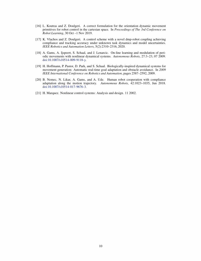
Comparing (6), (8)-(10) for the novel DMP with (26), (27)-(29) for the classical one it is straightfor-ward to verify their equivalence hence spacial scaling is preserved. However, it should be pointedout that in the classical DMP the spatial scaling term is ks = (g − y0)/(gd − yd,0) whereas in thenovel formulation we define it as ks = (g − y0)/(fp(xf )− fp(x0)). This two definitions for ks arequite similar considering that fp(xf ) ≈ gd and fp(x0) ≈ yd,0. In fact, the proposed spatial scalingis more consistent, as it applies the scaling w.r.t. the learned trajectory thus it guarantees that thescaled trajectory converges to the new target. In classical DMPs the addition of the goal attractorαzβz(g − y) and the gating function gf(x) are required to ensure this.

With the analysis conducted above, we have proven that the classical DMP given by (1) reduces to(30), which is almost identical to (6), with the exception that yd is replaced by fp given by (12).That is, in classical DMP, in order to track the desired trajectory, the forcing term (21) is learnedand used as feed-forward control input in a spring-damper dynamical system, i.e. the linear partof (1). In contrast, we learn only the desired position yd through fp. Then fp is spatially scaledaccording to the new target position g. Moreover, since fp is parameterized w.r.t. to the phasevariable x, temporal scaling is achieved by adjusting the evolution of x through (7). Consequently,the proposed formulation retains the desirable traits of DMP.

Appendix B - Proof that classical DMP are not reversible

In this section we will show that the classical DMP is not reversible. Specifically, by reversingthe canonical system’s evolution, the classical DMP will not produce the reverse trajectory of theforward one. Assume the position yd(t1), velocity vd(t1) and acceleration ad(t1) of a demonstratedtrajectory with duration τ , t1 ∈ [0, τ ]. For simplicity and without loss of generality we ignorespatial and temporal scaling and consider a linear canonical system (x = 1/τ ) that goes from 0 to1. Therefore, x = t1/τ and the learned forcing term (assuming negligible training error) will be:

gf(x)(gd − yd,0)fs(x) = τ2dad(t1)− αzβz(gd − pd(t1)) + αzτdvd(t1) (32)

During forward execution we have x = 1/τ , x(0) = 0, so x = t/τ . Therefore the DMP’s forcingterm is given by (32) with t1 = t and the demonstrated trajectory will be faithfully reproduced.During reverse execution we have x = −1/τ , x(0) = 1, so x = 1 − t/τ , therefore t1 = τ − t.Hence the reverse position trajectory is yrev(t) = pd(τ − t). Taking its time derivative yieldsthe reverse velocity yrev(t) = pd(τ − t) = −vd(τ − t) and the reverse acceleration trajectoryyrev(t) = pd(τ − t) = ad(τ − t). Notice that the sign of the reversed velocity is flipped. The DMP’sforcing term will be given by (32) with t1 = τ − t, hence on the right hand-side we get the incorrectterm αzτdvd(τ − t), instead of the correct one −αzτdvd(τ − t) with the correct sign of the reversevelocity. To understand the consequences of this, following the procedure given in Appendix A, theDMP’s equation eq. (1) can be written as:

(y − yrev(t)) +αz

τ(y − yrev(t)) +

αzβzτ2

(y − yrev(t)) = −2azτyrev(t) (33)

which clearly shows that the DMP output y, y, y will not track faithfully the reverse trajectory due tothe existence of the term −2az

τ yrev(t) at the right hand-side, which acts as a disturbance. Increasingthe stiffness improves the system’s robustness to disturbances but has several negative implications.Specifically, it is usually desirable to include additional coupling terms in order to shape the DMP’strajectory (e.g. for obstacle/limit avoidance, to make the DMP compliant to external forces etc). Ahigh stiffness would mitigate or even cancel the effectiveness of this desirable couplings. Moreover,if the goal or the DMP’s position y is perturbed, the high stiffness will incur high accelerations andin turn high velocities, which could violate the robot’s limits. Finally, a high K renders the DMP’sequation stiff, which can lead to numerical instability.

12

Appendix C - Unit Quaternion Preliminaries

Given a rotation matrix R ∈ SO(3), an orientation can be expressed in terms of the unit quaternionQ ∈ S

3 as Q = [w vT ]T = [cos(θ) sin(θ)kT ], where k ∈ R3, 2θ ∈ [0 2π) are the equivalent

unit axis - angle representation. The quaternion product between the unit quaternions Q1, Q2 is

Q1 ∗ Q2 =

[

w1w2 − vT1 v2

w1v2 + w2v1 + v1 × v2

]

. The inverse of a unit quaternion is equal to its conjugate

which is Q−1 = Q = [w − vT ]T . The quaternion logarithm is η = log(Q), where log : S3 → R

3

is defined as:

log(Q) ,

2 cos−1(w) v||v|| , |w|6= 1

[0, 0, 0]T , otherwise(34)

The quaternion exponential is Q = exp(η), where exp : R3 → S

3 is defined as:

exp(η) ,

[cos(||η/2||), sin(||η/2||) ηT

||η|| ]T , ||η||6= 0

[1, 0, 0, 0]T , otherwise(35)

If we limit the domain of the exponential map exp : R3 → S

3 to ||v||< π and the domain ofthe logarithmic map to S

3/([−1, 0, 0, 0]T ), then both mappings become one-to-one, continuouslydifferentiable and inverse to each other. The equations that relate the time derivative of η and therotational velocity ω and acceleration ω of Q are [16]:

η = JQ(Ω ∗Q) (36)

Ω = 2(Jηη) ∗ Q (37)

Ω = 2(Jηη + Jηη) ∗ Q−1

2

[

||ω||2

03×1

]

(38)

where Ω = [0 ωT ]T and

JQ = 2[

θ cos(θ)−sin(θ)sin2(θ) k θ

sin(θ)I3

]

(39)

Jη =1

2

[

− sin(θ)kT

sin(θ)θ (I3 − kkT ) + cos(θ)kkT

]

(40)

13