A Representative Irrigated Farming System in the Lower Namoi Valley of NSW:

An Economic Analysis

Janine Powell

Industry & Investment NSW, Australian Cotton Research Institute, Narrabri, NSW Cotton Catchment Communities CRC, Narrabri, NSW

Fiona Scott

Industry & Investment NSW, Tamworth Agricultural Institute, Tamworth, NSW

Economic Research Report No. 46

January 2011

1

Cotton Catchment Communities CRC 2011 This publication is copyright. Except as permitted under the Copyright Act 1968, no part of the publication may be reproduced by any process, electronic or otherwise, without the specific written permission of the copyright owner. Neither may information be stored electronically in any way whatever without such permission. Abstract This report presents a description of the Lower Namoi Valley of NSW and representative whole-farm budgets for the region based on subregional characteristics and the related farming systems. Agronomic and agricultural production characteristics are included as technical parameters in a transparent financial framework. A computer spreadsheet is developed to allow risk analysis of alternative technologies and management scenarios. Alternative crop rotations in a whole-farm context were compared. Keywords: Cotton; Irrigation; Whole farm model; Namoi Valley; economic; evaluation; Australia JEL Code: Q12, Q16 ISSN 1442-9764 ISBN 978 1 74256 063 2 Published by Industry & Investment NSW Senior Author's Contact: Janine Powell, Industry & Investment NSW, Locked Bag 1001, Narrabri, NSW, 2390. Telephone: (02) 6799 2469 Facsimile: (02) 6793 1171 Email: janine.powell@industry.nsw.gov.au Citation: Powell, J. and Scott, F. (2011), A Representative Irrigated Farming System in the Lower Namoi Valley of NSW: An Economic Analysis. Economic Research Report No. 46, Industry & Investment NSW, Narrabri, January. Internal reference: PUB11/14

2

Table of Contents Page

List of Tables .......................................................................................................................................................... 4 List of Figures ......................................................................................................................................................... 5 Acknowledgments................................................................................................................................................... 6 Acronyms and Abbreviations Used in the Report................................................................................................... 6 Executive Summary ................................................................................................................................................ 7

1. Introduction....................................................................................................................... 8 1.1 Use of Representative Farm Analysis............................................................................................................. 8

2. Namoi Valley ..................................................................................................................... 9 2.1 Physical characteristics of the region.............................................................................................................. 9 2.2 Climate ......................................................................................................................................................... 11 2.3 Land Use....................................................................................................................................................... 12

3. Irrigation.......................................................................................................................... 14

4. Irrigated crop selection................................................................................................... 16 4.1 Volatile commodity prices............................................................................................................................ 17 4.2 Soil health..................................................................................................................................................... 20 4.3 Pests and disease........................................................................................................................................... 21 4.4 Water supply................................................................................................................................................. 21 4.5 Climate Change ............................................................................................................................................ 22 4.6 Carbon .......................................................................................................................................................... 22

5. Cotton Industry ............................................................................................................... 22 5.1 Overview ...................................................................................................................................................... 22 5.2 Best Management Practices Program ........................................................................................................... 24

6. Representative Farm Model........................................................................................... 25 6.1 Resources...................................................................................................................................................... 25 6.2 Commodity Prices ........................................................................................................................................ 26 6.3 Rotational Crops........................................................................................................................................... 27 6.4 Financial Characteristics............................................................................................................................... 32

7. Results .............................................................................................................................. 33 7.1 Financial performance of the Representative Farm ...................................................................................... 33 7.2 Impact of price variability on whole farm returns ........................................................................................ 34

8. Application 1 – Rotation and tillage trials .................................................................... 36 8.1 Trial background .......................................................................................................................................... 36 8.2 Cotton rotation study .................................................................................................................................... 36 8.3 Methods ........................................................................................................................................................ 37 8.4 Results of the rotations ................................................................................................................................. 39

9. Conclusions ...................................................................................................................... 48 9.1 Representative farm...................................................................................................................................... 48 9.2 Whole farm impacts of rotations and tillage................................................................................................. 48

10. References ........................................................................................................................ 50

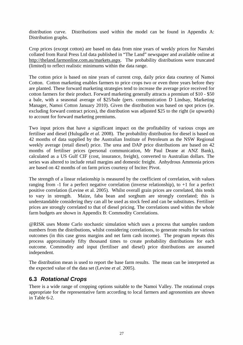
11. Appendix A: Distribution graphs .................................................................................. 54

12. Appendix B: Commodity Correlations ......................................................................... 56

13. Appendix C: Plant & Equipment Register ................................................................... 58

14. NSW Department of Industry and Investment Economic Research Report Series . 59

3

List of Tables Page

Table 2-1: Climate indicators Namoi Valley ........................................................................... 11 Table 2-2: Agricultural Land Use in the Namoi Valley - 2005/06 .......................................... 12 Table 3-1: Annual water extractions (GL) ............................................................................... 15 Table 3-2: Irrigation Water Use Index ..................................................................................... 16 Table 6-1: Resource Characteristics......................................................................................... 25 Table 6-2: Farming Enterprises................................................................................................ 28 Table 6-3: Probability of Gross Margin occurring below x$/ML............................................ 28 Table 6-4: Probability (%) of returning above x$/ML............................................................. 29 Table 6-5: Selected Irrigation Enterprises................................................................................ 31 Table 6-6: Selected Dryland Enterprises.................................................................................. 31 Table 6-7: Statement of Assets and Liabilities......................................................................... 32 Table 6-8: Whole Farm Budget................................................................................................ 33 Table 8-1: Experiment treatments ............................................................................................ 37 Table 8-2: Indicative Yields, Gross Margins and Water Use .................................................. 38 Table 8-3: Land allocated to rotational crop ............................................................................ 38 Table 8-4: Example of offset rotations.................................................................................... 38 Table 8-5: Area allocated to crop: Treatment 1 ....................................................................... 39 Table 8-6: Area allocated to crop: Treatment 2 ....................................................................... 40 Table 8-7: Area allocated to crop: Treatment 3 ....................................................................... 40 Table 8-8: Area allocated to crop: Treatment 4 ....................................................................... 41 Table 8-9: Financial Performance ............................................................................................ 42 Table 8-10: % Probability of Gross Margin result occurring below, above or between $500K and $700K ................................................................................................................................ 43 Table 12-1: Grain and legume price correlations..................................................................... 56 Table 12-2: Fertiliser and diesel price correlations .................................................................. 57

4

List of Figures Page

Figure 2.1: Map of the Namoi Catchment, NSW Australia ..................................................... 10 Figure 2.2: Mean Monthly Rainfall.......................................................................................... 11 Figure 2.3: 'Crops' breakdown, 2005/06 (ha) ........................................................................... 12 Figure 2.4: Irrigated Land Use, Namoi Valley 2005/06 (ha) ................................................... 13 Figure 2.5: Cotton Planting, Namoi Valley 2005/06 (ha) ........................................................ 13 Figure 3.1: Namoi Valley Account Balance, by Season .......................................................... 14 Figure 3.2: Irrigation Water Use Index Trend line................................................................... 16 Figure 4.1: Average Cotton price, $(AUD) per 227 kg bale of lint, Dec 2000 to Dec 2009 ... 17 Figure 4.2: Cereal prices, Narrabri, $(AUD) per tonne, Aug 2000 to Oct 2009...................... 18 Figure 4.3: Average Pulse prices, Narrabri, $(AUD) per tonne, Aug 2000 to June 2009 ....... 18 Figure 4.4: Fertiliser - Import Parity Prices ............................................................................. 19 Figure 4.5: Weekly Average Retail Diesel Price (NSW Regional Average)........................... 19 Figure 4.6: AUD/USD Exchange Rate .................................................................................... 20 Figure 5.1: Australian Cotton Production (ha harvested) ........................................................ 23 Figure 5.2: Comparative Cotton Yields by Country ................................................................ 23 Figure 5.3: Top 5 exporters of cotton....................................................................................... 24 Figure 6.1: Gross Margin Returns per megalitre...................................................................... 30 Figure 7.1: Net Farm Cash Income distribution....................................................................... 34 Figure 7.2: Farm Operating Surplus and Net Farm Cash Income............................................ 35 Figure 7.3: Return on Assets and Return on Equity................................................................. 35 Figure 8.1: Gross Margin comparison by treatment ................................................................ 43 Figure 8.2: Net farm cash income comparison ........................................................................ 44 Figure 8.3: Farm operating surplus comparison....................................................................... 44 Figure 8.4: Return on assets comparison (%) .......................................................................... 45 Figure 8.5: Return on equity comparison (%).......................................................................... 46 Figure 8.6: Sensitivity Charts (T1 to T4) ................................................................................. 47 Figure 11.1: Cotton lint price distribution................................................................................ 54 Figure 11.2: Cotton seed price distribution.............................................................................. 54 Figure 11.3: Chickpea price distribution.................................................................................. 54 Figure 11.4: Wheat price distribution ...................................................................................... 54 Figure 11.5: Faba bean price distribution................................................................................. 55 Figure 11.6: Maize price distribution....................................................................................... 55 Figure 11.7: Sorghum price distribution .................................................................................. 55 Figure 11.8: Anhydrous Ammonia price distribution .............................................................. 55 Figure 11.9: Di-Ammonium Phosphate (DAP) price distribution ........................................... 56 Figure 11.10: Urea price distribution ....................................................................................... 56 Figure 11.11: Diesel price distribution..................................................................................... 56

5

Acknowledgments The excellent cooperation of the management and staff of the Cotton Catchment Communities CRC, (also the funding body) is acknowledged. We also wish to acknowledge the considerable efforts of the Industry and Investment NSW cotton research and extension team, in particular Nilantha Hulugalle. In writing this report and developing the representative farm model we benefited greatly from discussions with Namoi Valley farmers and agribusiness advisers. Of particular help was a group that helped to define the characteristics of a typical farm by reaching a consensus in a meeting. This involved PJ Gileppa (Auscot), Ross Brown (Namoi Cotton), Elle MacPherson (Steve Madden Agriculture), Christian Powell (Cotton Grower) and Tom Wilson (Cotton Grower). Critical review and comments by Tom Nordblom and Rod Jackson (both of I&I NSW) are also gratefully acknowledged.

Acronyms and Abbreviations Used in the Report AA Anhydrous Ammonia

ABARE Australian Bureau of Agricultural and Resource Economics

ABS Australian Bureau of Statistics

AIP Australian Institute of Petroleum

ANRA Australian Natural Resources Atlas

ASW Australian standard white (this is a common wheat grade)

AUD Australian Dollar

BOM Bureau of Meteorology

BT Bacillus thuringiensis (genetically engineered cotton plants have insect tolerance by expressing crystal proteins genes from B. thuringiensis. When insects ingest toxin crystals the alkaline pH of their digestive tract causes the toxin to become activated.)

BMP Best Management Practice

CIF Cost Insurance Freight

Cotton CRC Cotton Catchment Communities Cooperative Research Centre

CRDC Cotton Research and Development Corporation

CSIRO Commonwealth Scientific and Industrial Research Organisation

DAP Di-Ammonium Phosphate

ETS Emissions trading scheme

GL Giga litre (1 million cubic metres or 1,000 ML, water volume)

GM Gross Margin

I&I NSW Industry and Investment NSW (formerly the NSW Department of Primary industries)

IWUI Irrigation Water Use Efficiency

ML Mega litre (1,000 cubic metres or 1 million litres, water volume)

NSW New South Wales

ROA Return on assets

ROE Return on equity

USD United States Dollar

6

Executive Summary This report presents a description of a whole-farm budget for a representative farm in the Lower Namoi Valley. This is used to give a ‘snapshot’ of the financial performance of the model farm and to analyse the financial implications of changes in cropping rotations or changes in management practice. The representative farm model is based on available data, local consensus and assumptions about the size of a typical farm and other resources such as labour, overhead costs, assets and liabilities and the nature of the cropping rotation used. The whole farm budget was constructed from these assumptions and from information on enterprise gross margin budgets. The whole farm budget provides an indication of the financial performance at a particular point in time of a farm with a particular set of resources. Within this analysis water resources were severely restricted to reflect license allocations at the time. While the representative farm model presented in this Report may give a broad indication of the financial performance of many farms in the Lower Namoi Valley, it may be quite different for farms with markedly different resources or enterprise rotations to those of the representative farm. Apart from providing a broad brush picture of financial performance, the model was used to analyse comparisons of alternative crop rotations in a whole-farm context. While simple gross margin analyses are useful at the enterprise scale, invariably a more thorough analysis at the whole farm scale is required to assess financial impacts of different cropping rotations over a longer period. Results from the representative farm budgets for the Lower Namoi Valley indicate that even with restricted water entitlements the business would return an operating surplus of $152,070. This is equivalent to a return on equity of 3.1 per cent. The representative farm is vulnerable to commodity price variability. Results suggest that one year in five, the farm is unlikely to return a positive cash surplus. Using the model to compare four rotational trials highlighted the importance of crop selection for the financial performance of the business. Mean results indicated a positive return for all rotations within the representative farm budgets for the Lower Namoi Valley. Farm operating surplus ranged from $177,715 to $374,755 indicating that given restricted irrigation water and average commodity prices each rotation would ensure that the business returned a profit. The rotations varied in resilience to commodity variability, however all treatments were likely to return a profit with the worst performing treatment at a 96% probability to return a positive farm operating surplus. An important objective of our work was to develop some tools which can help in assessing the change in farm profit from new ideas and technologies generated by the research and advisory activities of Industry and Investment NSW. The models can also be used to give an assessment of the impact on farm profit of policy changes with respect to the management of natural resources. Our work has been aimed at developing whole-farm representations or models that can be utilised, by researchers and extension officers, to assess potential changes. Such models can be used in at least two ways – to rank technologies and management practices while they are

7

being developed or prior to release, and as a tool to strengthen extension programs by demonstrating to farmers that there may be sufficient financial advantage in a technology to warrant adoption. Of course we acknowledge that there are other aspects of new technologies (apart from the financial) that influence adoption decisions. We hope that economic analyses at the enterprise and farm levels will provide information which assists sound decision making.

1. Introduction It is important to understand the farm level impacts of cotton industry research. Our objective in this report is to describe how farmers in the Lower Namoi Valley typically combine crop and livestock enterprises in a whole farm context and to assess the financial performance of such farming systems. This is achieved by the development of a whole-farm budget for a representative farm. The resulting whole-farm budget is used to give a snapshot of the financial performance of the model farm and to analyse the financial implications of changes in cropping rotations. These models can be used to analyse changes in farm profit from other technologies or changes in policy with respect to the management of natural resources. Farm decision makers may have several objectives which they try to achieve simultaneously. Other than an economic return, objectives to ensure the long term sustainability of the farm may include management of soils, pests, weeds & disease. Economic evaluations of alternative technologies use profits as the primary incentive for decisions, because this is considered to be an important consideration for many farm decision makers. The farm model presented here assumes the profit objective. However, we recognise that this is not the only possible motivation, and consider the results of such analyses to be only partial in providing information to farmers. Financial budgeting can be used to estimate the change in profits from new technologies or management strategies. Profit changes can be considered at the enterprise level (eg gross margin budgets for alternative crops, partial budgets, cash flow budgets), for crop sequences (eg winter and summer crop sequence budgets), and at the whole-farm level. Enterprise and whole-farm budgets are presented in this report to represent a common farming system in the Namoi Valley. However, all models are simplified representations of reality. The value of a model depends on how it is used, and the results of analysis with models need to be interpreted carefully.

1.1 Use of Representative Farm Analysis A whole farm budget was developed for the Lower Namoi Valley. It is broadly representative of a typical farming system within the region, although we must be careful when interpreting the results for individual farms. We propose that the model be used as the basis for face-to-face discussions and interaction between researchers, advisors and farmers. This would include generating and analysing ‘what if’ scenarios. Chapter 8 also contains an example application of the model to a particular farming system. The results from such analyses, together with personal interactions will hopefully lead to improved understandings on the part of all participants. The models and model results are a means to an end of improved knowledge and communication, rather than ends in themselves. This Report presents a description of an irrigated farming system in the Lower Namoi Valley region of NSW and an indication of its profitability and financial viability. The representative

8

9

farm model and associated gross margin and whole farm budgets can be used as templates allowing variations from the representative farm model to be examined. The whole farm budget provides a snapshot at a particular point in time of a farm with a particular set of resources. Hence while this report may give a broad indication of what is happening on many farms in the northern cropping region of NSW, it may be inaccurate for farms with markedly different soil type, climate and resources to those of the representative farm. Additionally while the whole farm budget can be manipulated to indicate the change in farm income from a new technology or resource management strategy, again we only get before and after pictures. If, for example, the change in technology has an impact on soil fertility that may take many years to work through the system, then a simple before and after comparison of whole farm budgets is an inadequate basis for such an important investment decision. More sophisticated budgeting tools that allow the impact of such changes over many years to be estimated and aggregated may be required, such as cash flow development budgets.

2. Namoi Valley

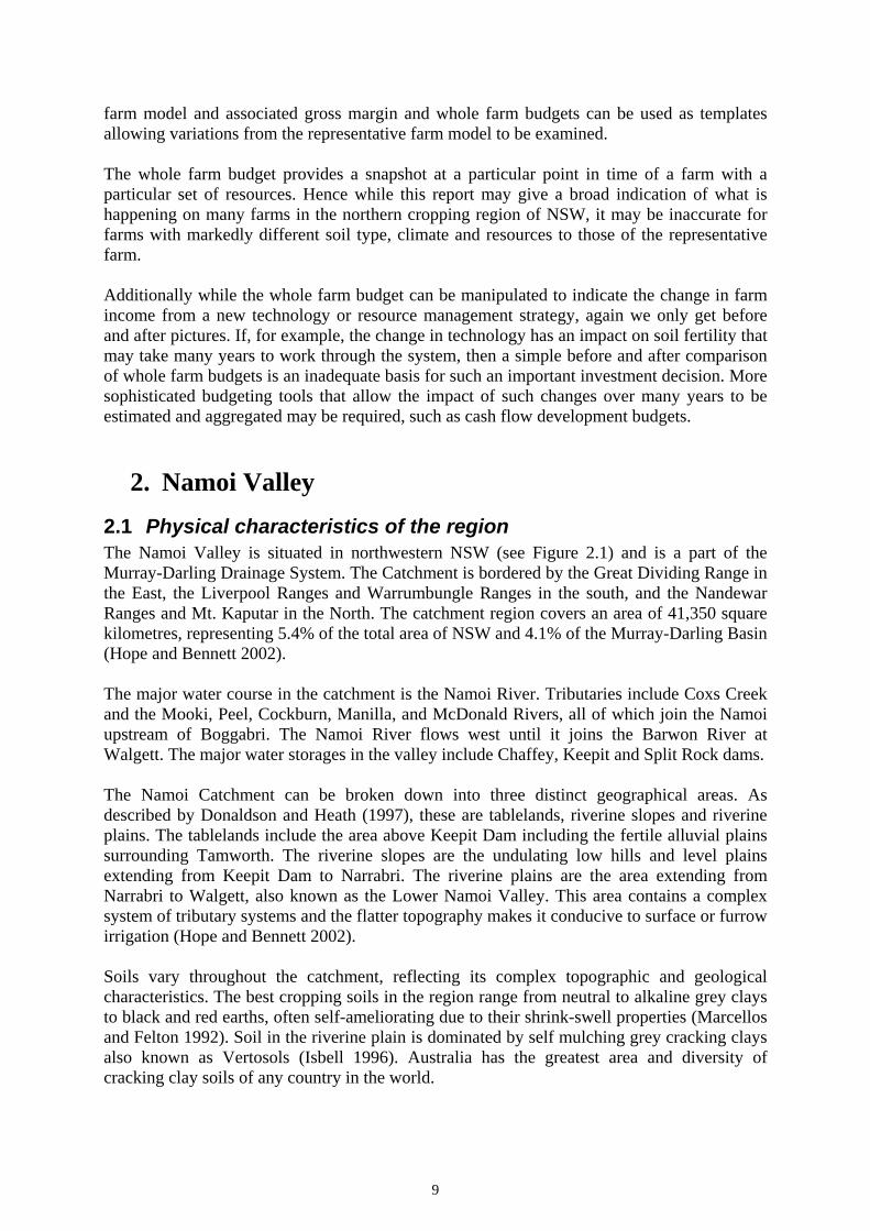
2.1 Physical characteristics of the region The Namoi Valley is situated in northwestern NSW (see Figure 2.1) and is a part of the Murray-Darling Drainage System. The Catchment is bordered by the Great Dividing Range in the East, the Liverpool Ranges and Warrumbungle Ranges in the south, and the Nandewar Ranges and Mt. Kaputar in the North. The catchment region covers an area of 41,350 square kilometres, representing 5.4% of the total area of NSW and 4.1% of the Murray-Darling Basin (Hope and Bennett 2002). The major water course in the catchment is the Namoi River. Tributaries include Coxs Creek and the Mooki, Peel, Cockburn, Manilla, and McDonald Rivers, all of which join the Namoi upstream of Boggabri. The Namoi River flows west until it joins the Barwon River at Walgett. The major water storages in the valley include Chaffey, Keepit and Split Rock dams. The Namoi Catchment can be broken down into three distinct geographical areas. As described by Donaldson and Heath (1997), these are tablelands, riverine slopes and riverine plains. The tablelands include the area above Keepit Dam including the fertile alluvial plains surrounding Tamworth. The riverine slopes are the undulating low hills and level plains extending from Keepit Dam to Narrabri. The riverine plains are the area extending from Narrabri to Walgett, also known as the Lower Namoi Valley. This area contains a complex system of tributary systems and the flatter topography makes it conducive to surface or furrow irrigation (Hope and Bennett 2002). Soils vary throughout the catchment, reflecting its complex topographic and geological characteristics. The best cropping soils in the region range from neutral to alkaline grey clays to black and red earths, often self-ameliorating due to their shrink-swell properties (Marcellos and Felton 1992). Soil in the riverine plain is dominated by self mulching grey cracking clays also known as Vertosols (Isbell 1996). Australia has the greatest area and diversity of cracking clay soils of any country in the world.

Figure 2.1: Map of the Namoi Catchment, NSW Australia

Source: (Namoi CMA.)

10

2.2 Climate Climate characteristics vary from the tablelands to the riverine plains. In the upper slopes at Tamworth average summer temperatures range from 17.4°C to 31.9°C, in winter from 2.9°C to 15.5°C, whilst in Walgett summer temperatures range from 20.4°C to 35.4°C and in winter from 3.3°C to 18.3°C. Rainfall in the region is variable and decreases from east to west. Yearly averages range from approximately 470 mm in the riverine plains around Walgett to more than 800mm on the higher parts of the tablelands. Overall, rainfall is highest in the summer months, November through February (Figure 2.2), and usually consists of short duration heavy falls. Flooding in the catchment can occur both in summer and winter, however summer flooding is generally more severe.

Figure 2.2: Mean Monthly Rainfall

0

10

20

30

40

50

60

70

80

Jan Feb Mar Apr May Jun Jul Aug Sep Oct Nov Dec

Month

Rai

nfa

ll (m

m)

Tamworth Airport Walgett Airport

Data Source: (BOM 2009)

Frosts are common in the Namoi Catchment during winter, and some snowfalls occur on the tablelands. Frost incidence decreases from East to West.

Table 2-1: Climate indicators Namoi Valley

Tamworth Narrabri Walgett

(Tablelands) (Riverine

Slopes / Plains) (Riverine Plains)

Mean maximum temperature (°C) 24.3 26.5 27.5

Mean minimum temperature (°C) 10.2 11.7 11.9

Mean number of days > 35°C 14.1 unknown 63.9

Mean rainfall (mm/y) 673.2 657.1 440.6 Mean monthly Pan Evaporation (mm/day) * 5.4 6 6.6

Data Source: (BOM 2009)

11

2.3 Land Use The Namoi Catchment supports a variety of land uses. The first settlers in the Namoi Valley engaged in sheep and cattle grazing as well as wool production. As land was cleared, many of these enterprises diversified into dry land broad acre farming. Results from the 2005/06 Agricultural Census indicate land use continues to be dominated by the livestock and broad acre farming industries, as can be seen in Table 2.2.

Table 2-2: Agricultural Land Use in the Namoi Valley - 2005/06

Agricultural Land Use Ha

% of Total Area

Grazing 2,117,272 64%Crop / Fallow 949,783 29%Remnant vegetation and woodland 117,895 4%Not Reported 82,878 2%Houses, sheds and other agriculturally unproductive land 28,762 <1%Commercial forestry plantations 24,185 <1%Wetlands / swamps & other environmentally areas not suitable for grazing 8,798 <1%

Data Source:(ABS 2008)

The opening of Keepit Dam in October 1960 was followed by rapid development of an irrigated agriculture industry in the Namoi Valley with the first commercial cotton crop in the valley grown at Wee Waa in 1961. In the 2005/06 season, cotton was the fourth largest crop in terms of land use in the Catchment, accounting for 9% of total crop land (Figure 2.3).

Figure 2.3: 'Crops' breakdown, 2005/06 (ha)

Oilseeds4%Oats

3%

Maize1%

Legumes4%

Wheat41%

Sorghum19%

Barley15%

Pastures & crops cut for

hay4%

Cotton9%

Data Source: (ABS 2008)

12

In terms of irrigated land use, cotton has been the dominant crop planted for irrigation in the Namoi Valley. According to the ABS (2008), in 2005/06 cotton dominated irrigated land use in the Valley, accounting for 61% of the irrigated crop area (Figure 2.4).

Figure 2.4: Irrigated Land Use, Namoi Valley 2005/06 (ha)

Crops for hay & silage9%Pasture for

grazing6%

Other broadacre

crops3%

Cotton61%

Cereal crops21%

Data Source: (ABS 2008)

According to the ABS (2008), in the 2005-06 season in the Namoi Valley there were approximately 94,000 hectares of irrigated area operated by 701 businesses. In the same season, Cotton Australia (2006) estimated there were 140 businesses growing cotton on 57,000 hectares in the Namoi Valley. Among these, 100 businesses and 44,000 hectares were in the Lower Namoi Valley (Figure 2.5).

Figure 2.5: Cotton Planting, Namoi Valley 2003/04 to 2008/09 (ha)

21200

12372

21050

44000

40000

10000

7450

7377

10750

13000

12000

10000

0 10000 20000 30000 40000 50000 60000

2008/09

2007/08

2006/07

2005/06

2004/05

2003/04

Sea

son

Area of Cotton Planted (ha)

Lower Namoi Upper Namoi

Data Source: Cotton Australia Annual Reports (2004), (2005), (2006), (2007), (2008), (2009)

13

3. Irrigation The Namoi Valley is unusual in the fact that it has several irrigation water sources including groundwater, regulated river, supplemented flows and unregulated rivers (Baillie et al. 2008). The Namoi River is regulated by Keepit Dam which was the first major water supply dam constructed in the Northern Murray Darling Basin and has a storage capacity of 423,000 megalitres (ML). Split Rock Dam on the Manilla River has a storage capacity of 397,000 ML (ANRA 2009). Chaffey Dam in the south-east of the catchment supplies irrigators on the Peel River with a capacity of 62,000 ML. Regulated water in the catchment is broken into three sections; the regulated sections of the Peel River, Upper Namoi and Lower Namoi sections of the Namoi River. The regulated sections of the Lower Namoi include downstream of Keepit Dam to the Barwon River, including the regulated sections of the Gunidgera/Pian system. Regulated surface water licences are managed by the NSW State Government and seasonal allocations are announced periodically as inflows occur. Continuous accounting (introduced in 1999), allows carryover of unused seasonal allocation. The continuous accounting system currently has a limit of 200% of the licensed entitlement. Prolonged drought has reduced water available for irrigation. Since 2002 the long term average seasonal balance for regulated surface water licences on the Namoi River has been 25%. Coincidentally in September 2009 the balance was also 25% (Figure 3.1).

Figure 3.1: Namoi Valley Account Balance, by Season

0%

20%

40%

60%

80%

100%

31/1

0/20

02

28/0

2/20

03

30/0

6/20

03

31/1

0/20

03

29/0

2/20

04

30/0

6/20

04

31/1

0/20

04

28/0

2/20

05

30/0

6/20

05

31/1

0/20

05

28/0

2/20

06

30/0

6/20

06

31/1

0/20

06

28/0

2/20

07

30/0

6/20

07

31/1

0/20

07

29/0

2/20

08

30/0

6/20

08

31/1

0/20

08

28/0

2/20

09

30/0

6/20

09

Date

Val

ley

Acc

ount

Bal

ance

(%)

2002/2003 2003/2004 2004/2005 2005/2006

2006/2007 2007/2008 2008/2009 2009/2010

Data Source: http://www.waterinfo.nsw.gov.au/ac

Many Namoi irrigation enterprises have adapted to supply variability by investing in water storage infrastructure. Both regulated and unregulated water licence holders have invested in on farm water storages to harvest storm water, capture off allocation flows (supplementary water), and to buffer against supply interruptions. In addition to these surface water resources, the Namoi valley has also a number of groundwater aquifers that provide a significant source

14

of irrigation water (see Table 3-1 below). The reliance on these groundwater resources for agricultural production is especially high during times of low river allocations. In the nine seasons from 2000/01 to 2008/09, an average of 209 gigalitres (GL) of river diversions and an average of 210 GL of groundwater was extracted by irrigators in the Namoi Valley (Table 3-1). The Namoi Valley is the only valley in the Murray Darling Basin to have such similar water use of groundwater and river water, with most areas having access and thus reliance on either river or ground water.

Table 3-1: Annual water extractions (GL)

Namoi Valley 2000/1 2001/2 2002/3 2003/4 2004/5 2005/6 2006/7 2007/8 2008/9 Avg Regulated (Lower & Upper Namoi) 182 266 194 30 62 141 114 39 61 121 Regulated (Peel) 7 15 22 13 11 15 ND ND ND 14 Supplementary 48 0 0 52 35 18 0 29 63 27 Unregulated 78 78 78 78 78 78 ND ND ND 78 Total River Diversions 315 359 294 173 186 252 114 68 124 209 Groundwater 279 253 246 199 183 165 253 187 146 212

Data Source: 2006/07 to 2008/09 (DWE 2009), 2000/01 to 2005/06 (Baillie et al. 2008) ND = No data

Furrow irrigation remains the dominant irrigation method for the industry. Furrow irrigation is where syphons are set by hand for each irrigation to draw water from the channel into every second contoured furrow (Roth 2006). Whilst other irrigation methods such as overhead and drip are more water use-efficient, the significant capital cost of conversion has been a barrier for most irrigation enterprises. There are other methods to improve water use efficiency (WUE), 72% of respondents of the Cotton Consultants Australia post season survey (2008) responded that they had implemented management practice changes to improve WUE. Types of improvements included;

- Utilising an objective irrigation scheduling technique - Evaluating surface irrigation performance with Irrimate - Determining storage efficiency - Installing water meters

The industry’s improving WUE is evident by the improvement in the ‘Irrigation Water Use Index’ (IWUI), which is the number of bales produced by the industry divided by the volume of water used by the industry. In the six seasons from 2002-03 to 2008-09, there was 39% improvement by the cotton industry (Table 3-2). It is important to note that IWUI is influenced by seasonal conditions, with the volume of water applied to a cotton crop very dependant on the amount of in crop rain fall. Despite seasonal considerations, the trend indicates definite improvements in IWUI over time (Figure 3.2).

15

Table 3-2: Irrigation Water Use Index

Cotton Season

Irrigated Production

(227kg bale)

Volume of Water

Applied (ML)

IWUI (bales/ML)

IWUI Change

from previous season

IWUI Change

from 2002-03

2002-03 1,766,090 1,525,504 1.16 2003-04 1,554,718 1,248,924 1.24 8% 8% 2004-05 2,598,392 1,819,315 1.43 15% 23% 2005-06 2,410,037 1,746,386 1.38 -3% 19% 2006-07 1,240,100 867,662 1.43 4% 23%

2007-08 568,330 309,442 1.84 29% 59%

2008-09 1,416,800 880,003 1.61 -13% 39% Production Data Source: The Australian Cotton Grower Yearbooks (2003; 2004; 2005; 2006; 2007; 2008) Water Consumption Data Source: (ABS 2009)

Figure 3.2: Irrigation Water Use Index Trend line

0.00

0.50

1.00

1.50

2.00

2002-03 2003-04 2004-05 2005-06 2006-07 2007-08 2008-09

Cotton Season

IWU

I (b

ales

/ML

)

4. Irrigated crop selection Choosing rotations for a farming system is a complex decision making process. Managing limited and specific resources, volatile input and output prices whilst maintaining soil health and ensuring the long term sustainability and profitability of a farming business is a challenging task. Some of the things farmers need to consider when choosing which crops to plant include; climate, soil type, soil structure, soil moisture, insect pressure, weed pressure, disease pressure, nutrition, cash flow requirements, water availability and available resources. Traditionally, typical cotton rotations involved cotton with winter fallow planted year after year, sometimes with a wheat crop planted (S. Madden, Steve Madden Agriculture, pers. comm., 2009). These rotations in time began to impact adversely on cotton yields due to declining soil fertility.

16

In response cotton farming system research has focussed on many areas including an understanding soil health and its impact on long term farm sustainability. Today cotton rotations have diversified to include green manure legume crops as well as pulse and cereal crops (Hulugalle and Scott 2008). With the recent volatility in general commodity prices, and the prolonged period of limited water there are no ‘typical’ rotations in an irrigated farming system. Farmers are choosing crops season by season depending on available water, current commodity prices, pest and disease pressure and various soil health issues.

4.1 Volatile commodity prices Recent exchange rate and commodity price volatility has added an extra consideration to the decision making process for irrigation farmers. In the past three years fertiliser, diesel and most grain crop prices have seen record highs before returning closer to long-term average levels. It is important to recognise that different rotations vary in terms of resilience to fluctuations of input prices (Hulugalle and Scott 2008).

Figure 4.1: Average Cotton price, $(AUD) per 227 kg bale of lint, Dec 2000 to Dec 2009

$250

$300

$350

$400

$450

$500

$550

$600

$650

12/1

0/00

12/0

2/01

12/0

6/01

12/1

0/01

12/0

2/02

12/0

6/02

12/1

0/02

12/0

2/03

12/0

6/03

12/1

0/03

12/0

2/04

12/0

6/04

12/1

0/04

12/0

2/05

12/0

6/05

12/1

0/05

12/0

2/06

12/0

6/06

12/1

0/06

12/0

2/07

12/0

6/07

12/1

0/07

12/0

2/08

12/0

6/08

12/1

0/08

12/0

2/09

12/0

6/09

$/ba

le (

227k

g lin

t)

Data: Namoi Cotton Co-operative

In the past nine years cotton prices have ranged from approximately $300/bale to $600/bale. Figure 4.1 charts the cotton price available for the ‘current’ season (prices farmers are offered when they are pricing the crop soon to be planted or already in the ground), it does not show prices that were offered to farmers to market forward (future year) cotton crops. Until recently, the past five years has provided limited opportunities for cotton farmers to market their crop above $450/bale. The effect on whole farm profit by pricing at $350/bale compared to $450/bale is significant. Increased input prices and depressed cotton prices have resulted in a cost-price squeeze for the cotton industry (Roth 2006). When cotton is trading under $350/bale, other irrigated crops may be more attractive in terms of return per ML or hectare.

17

Figure 4.2: Cereal prices, Narrabri, $(AUD) per tonne, Aug 2000 to Oct 2009

-

50

100

150

200

250

300

350

400

450

5002/

08/2

000

30/1

1/20

00

30/0

3/20

01

28/0

7/20

01

25/1

1/20

01

25/0

3/20

02

23/0

7/20

02

20/1

1/20

02

20/0

3/20

03

18/0

7/20

03

15/1

1/20

03

14/0

3/20

04

12/0

7/20

04

9/11

/200

4

9/03

/200

5

7/07

/200

5

4/11

/200

5

4/03

/200

6

2/07

/200

6

30/1

0/20

06

27/0

2/20

07

27/0

6/20

07

25/1

0/20

07

22/0

2/20

08

21/0

6/20

08

19/1

0/20

08

16/0

2/20

09

16/0

6/20

09

14/1

0/20

09

$/t

Wheat ASW Stockfeed Sorghum Maize

Data Source: Rural Press Ltd

In the past nine years, cereal prices have also been volatile (Figure 4.2). The ASW stockfeed wheat price in Narrabri has ranged from a low of $132/t to a high of $435/t, sorghum prices ranged from $107/t to $432/t and maize prices have ranged between $160/t and $458/t. Pulse prices have experienced similar pricing fluctuations with prices in the Narrabri area for chickpea ranging from $215/t to $710/t and faba bean from a low of $178/t to $650/t (Figure 4.3). Whilst prices of substitutable commodities are generally strongly correlated (an indication of the strength of relationship between two variables), there are times when one crop will clearly out perform the others in terms of return per hectare or return per ML.

Figure 4.3: Average Pulse prices, Narrabri, $(AUD) per tonne, Aug 2000 to June 2009

-

100

200

300

400

500

600

700

800

2/08

/200

0

30/1

1/20

00

30/0

3/20

01

28/0

7/20

01

25/1

1/20

01

25/0

3/20

02

23/0

7/20

02

20/1

1/20

02

20/0

3/20

03

18/0

7/20

03

15/1

1/20

03

14/0

3/20

04

12/0

7/20

04

9/11

/200

4

9/03

/200

5

7/07

/200

5

4/11

/200

5

4/03

/200

6

2/07

/200

6

30/1

0/20

06

27/0

2/20

07

27/0

6/20

07

25/1

0/20

07

22/0

2/20

08

21/0

6/20

08

19/1

0/20

08

16/0

2/20

09

16/0

6/20

09

14/1

0/20

09

$/t

Faba Beans Chickpeas

Data Source: Rural Press Ltd

Enterprise gross margins are also directly affected by fertiliser price fluctuations, depending on the amount of fertilisers used. Figure 4.4 shows import parity prices for fertiliser (urea and di-ammonium phosphate (DAP)). These prices, compiled by Mr Paul Deane at ANZ Bank, are calculated as a US Gulf CIF (includes cost, insurance, freight), converted to Australian

18

dollars. It does not include Australian wholesale or retail margins or freight charges. The urea import parity prices peaked at $1020/t in September 2008. ABARE (2008) reported the average price paid by Australian farmers in 2008 for urea as $852/t, a 66% increase on the previous years average of $512/t. DAP import parity prices peaked at $1530 in September 2008, with the average price paid by Australian farmers in 2008, $1353/t, which was a 108% increase on the average price paid in 2007.

Figure 4.4: Fertiliser - Import Parity Prices

200

400

600

800

1000

1200

1400

1600

Feb-06 Aug-06 Feb-07 Aug-07 Feb-08 Aug-08 Feb-09 Aug-09

Date

Pri

ce ($A

UD

/ t)

UREA DAP

Data Source: (ANZ 2009)

Diesel prices also affect enterprise gross margins and depending on the number of tractor hours for each enterprise and if diesel-powered irrigation pumps are used. Weekly NSW regional average diesel prices collated by the Australian Institute of Petroleum (AIP 2009) in the past four years show a high of 191.2c/l in July 2008, before falling 27% to a low of 121.2c/l in May 2009 (Figure 4.5).

Figure 4.5: Weekly Average Retail Diesel Price (NSW Regional Average)

100

120

140

160

180

200

Feb-06 Aug-06 Feb-07 Aug-07 Feb-08 Aug-08 Feb-09 Aug-09Date

Pri

ce (

cen

ts p

er li

tre)

Data Source: (AIP 2009)

Farm gate prices and profits are largely determined by world prices and the value of the Australian dollar (ABARE 1997). The prices of many of the commodities discussed in the

19

whole farm budgets are based on international prices, hence the Australian farm gate price is strongly influenced by the exchange rate. Exchange rate (AUD/USD) movements have an inverse relationship with AUD pricing. As the AUD strengthens, commodity prices offered to farmers weaken. A high exchange rate is not favourable in terms of output commodities (cotton, grain & pulses) due to the decrease in income received, however a high exchange rate is favourable in terms of imported input commodities (i.e. fertiliser and diesel), resulting in a reduction in receipts paid. The past two years have been a volatile period, with the AUD currently trading close to the levels seen since late 2007 (Figure 4.6).

Figure 4.6: AUD/USD Exchange Rate

0.4000

0.5000

0.6000

0.7000

0.8000

0.9000

1.0000

3/10

/200

0

3/04

/200

1

3/10

/200

1

3/04

/200

2

3/10

/200

2

3/04

/200

3

3/10

/200

3

3/04

/200

4

3/10

/200

4

3/04

/200

5

3/10

/200

5

3/04

/200

6

3/10

/200

6

3/04

/200

7

3/10

/200

7

3/04

/200

8

3/10

/200

8

3/04

/200

9

3/10

/200

9

Data Source: (RBA 2009)

4.2 Soil health Soil health has long term implications on farm profit and sustainability. Rotation choice can affect a number of soil factors including soil organic matter and the amount of nitrogen fixed in the soil (Cotton CRC 2008). Vetch for example, is a winter growing legume that is grown for its nitrogen fixing abilities. Like all legumes, vetch has a symbiotic relationship with rhizobia bacteria, which inhabit nodules formed on the roots of the plant. The rhizobia bacteria convert atmospheric nitrogen to a form which is used by the vetch plant for growth. Nitrogen-rich residues left by the crop contribute to the supply of nitrogen in the soil which is then available for subsequent crops to use (Rochester 2004). Grown as a green manure crop, the vetch plants are worked into the ground when the crop is still green and before viable seed is produced. There is no commodity harvested and no direct income from the crop. The benefit of growing vetch is the improvement of soil health by increasing organic matter and the amount of nitrogen in the soil, there is also evidence of increased yields of cotton crops grown after vetch crops (Cotton CRC 2008).

Legumes that produce a grain crop are known as pulse crops. Pulse crops are able to 'fix' nitrogen via root nodules populated with rhizobia bacteria and although most of this is stored in the grain and therefore removed when the crop is harvested, the plants have not taken this nitrogen from the soil and so the need for nitrogen fertilizers for subsequent crops is reduced (Rochester and Peoples 2005). The combination of higher soil nitrogen left after the crop and reduced root diseases is cumulative and can result in an increase in subsequent cereal yields

20

(Pulse Australia 2009). Recent work from southern Queensland has indicated that some residual nitrogen may remain in the soil after the pulse crop is removed, chickpea and mungbean contributed an average of 35 and 29 kg N/ha respectively in a field trial (Cox et al. 2010) forthcoming).

The majority of findings from studies on the benefits of using pulses in rotations indicated that when they are grown in rotation with cereal and oilseed crops, yields are increased by 0.5 to 1 tonne per hectare and protein by as much as 0.5 to 1.8% (Pulse Australia, 2009).

Compatibility with other rotation crops is a simple yet critical consideration. Canola residue is known to have an allelopathic (inhibitory) effect on a cotton crop planted immediately after canola harvest, potentially reducing cotton seedling vigour and cotton yield (Cotton CRC and CRDC 2009).

4.3 Pests and disease Breaking pest and disease cycles is an important factor in the selection of a suitable rotation for any farming system. Selecting rotations that strategically allow the control of problem weeds, insects and diseases is important. In terms of weeds, it is difficult to control grasses such as black oats in wheat and broadleaf weeds such as wild turnip in chickpea and faba bean. Pests such as aphids and whiteflies can be managed by choosing rotations that are not an attractive host (Cotton CRC and CRDC 2009). The careful selection of rotational crops is one tool for managing cotton disease. Evidence suggests adding cereals into a cotton rotation may decrease the severity of the disease verticillium wilt, whilst legume crops may increase the presence of black root rot in the following cotton crop (Cotton CRC and CRDC 2009).

4.4 Water supply The amount of irrigation water available has a large influence on which crops and the area to plant to an irrigation rotation system. Different crops use different amounts of irrigation water, however selecting the crop that uses the least amount of water is not necessarily the solution. With limited rainfall, low river allocations and reductions in groundwater entitlement, in recent years water has been the most limiting resource in an irrigated farming system. To ensure the greatest return, a business needs to maximise the return of the scarcest resource. In this case, farmers should choose crops based on those with the highest return per ML of water. If land was the scarcest resource, the farmer would look at return per hectare. One method used to utilise limited water is to deficit-irrigate crops. Deficit irrigation is a water management strategy that deliberately reduces the water available to the crop. Reduced yield under deficit-irrigation, may be compensated by an increased area of production (Ali et al. 2007). Depending on various commodity prices, at times it may be more profitable to deficit-irrigate one crop rather than fully irrigate another (Payero and Harris 2008). However, this requires careful management and good knowledge of how a crop will respond to deficit-irrigation. Cotton, for example, is highly responsive to water. A crop that has been deficit-irrigated may also be referred to as semi-irrigated. Due to water shortages, it has also become more common for farms to grow dryland crops on paddocks that were previously used for irrigated crops. These crops receive reduced inputs and no irrigation water. This allows a farmer to utilise a paddock that would have otherwise been fallow due to lack of irrigation water.

21

4.5 Climate Change Climate change is expected to adversely affect weather in Australia with warmer temperatures, declining rainfall and higher incidence of extreme weather events including, droughts extreme rainfall and bushfires (CSIRO 2006). By 2030, CSIRO (2006) predicts average temperatures in the Namoi valley to increase as much as 2.1oC, and rainfall to decrease by up to 13%. These changes along with associated higher evaporation are likely to lead to less water in the rivers and streams, which would constrain future irrigation allocations and significantly reduce dryland farming yields. Livestock enterprises are also expected to be adversely affected with a likely increase in heat stress (CSIRO 2006). The sustainability of an irrigation farming system will depend on the businesses adaptability to farm in this hotter and drier environment.

4.6 Carbon The long term profitability of irrigation farming systems is likely to be affected by evolving Australian government policy and continuing global discussion in terms of carbon. If an emissions trading scheme (ETS) were to be introduced into Australia the effect on farmers would depend on the level of inclusion of agriculture. If agriculture was excluded, gross margins would still be affected by an increase in various input prices, where industries affected pass on any costs to the consumer (Tulloh et al. 2009). If the agricultural sector were to be included within the ETS, there may be potential economic benefits for carbon sequestration in soils. The combination of these factors may have an impact on the profitability of future irrigation and dryland crops, however, a full assessment of the impact of the proposed ETS scheme is beyond the scope of this report.

5. Cotton Industry

5.1 Overview From its infancy in the 1960’s, the Australian cotton industry developed for 30 years before peaking in the 1998-99 cotton season with 561 thousand hectares harvested. Most cotton growing areas in Australia recently experienced severe drought, which is reflected in the reduced cotton area during 2006-07 and 2007-08. Due to increases in yield per hectare, the peak of lint production was in 2000-01 when 819 kilotonnes (3.61 million 227 kilo bales) were produced.

22

Figure 5.1: Australian Cotton Production (ha harvested)

0

100

200

300

400

500

600

1961-62

1963-64

1965-66

1967-68

1969-70

1971-72

1973-74

1975-76

1977-78

1979-80

1981-82

1983-84

1985-86

1987-88

1989-90

1991-92

1993-94

1995-96

1997-98

1999-00

2001-02

2003-04

2005-06

2007-08

Cotton Season

'000

ha

Data Source: (ABARE 2008)

Figure 5.2: Comparative Cotton Yields by Country

0

500

1000

1500

2000

2500

2000 2001 2002 2003 2004 2005 2006 2007 2008 2009

Cotton Season

kg

/ h

a

Australia Israel SyriaBrazil China World Average

Data Source: (ABARE 2008)

As the world leader in terms of cotton yield per hectare, Australia’s average yield in 2008 season was 2.12 t/ha or 9.34 bales/ha (ABARE 2008). World average cotton yields have increased from an estimated 141 kg/ha in 1973-74 to a high of 796 kg/ha in 2007-08. Australian yields are consistently higher than all cotton producing nations as shown in Figure 5.2.

23

Figure 5.3: Top 5 exporters of cotton

0

5

10

15

20

25

30

2000 2001 2002 2003 2004 2005 2006 2007 2008 2009

Cotton Season

mil

lion

480

lb b

ales

USA India Australia Brazil Greece

Data Source: (USDA 2009) In the past ten years, Australia’s market share of world exports has declined significantly from 15% of world cotton exports in 2000 to an estimated 5% in 2009. The decline in Australia’s export status is directly linked to the diminished production due to drought conditions in Australia’s cotton growing regions. During the same period, India’s exports increased from less than 1% of world cotton exports to an estimated 20% in 2009 (Powell 2009). The emergence of India as a major exporter is largely due to the significant increase in their cotton production. From 2000 to 2009 India’s production increased from 12.3 million to 23.5 million bales with the increase mainly attributed to a rise in yields since the introduction of BT cotton (Bennett et al.).

5.2 Best Management Practices Program The cotton industry’s Best Management Practices (BMP) program is a voluntary farm management system. The aim of the program is to “achieve sustainability through improved farm efficiency and productivity along with protecting the environment and its natural resources”. The program provides information and practical tools across a range of farm management areas including; Human Resources, Biosecurity, Soil Health, IPM, Greenhouse and Carbon, Water Management, Natural Resource Assets, Quality, Pesticide Management, Petrochemicals, Technology (Cotton Australia 2008). Also provided within the program are self assessment mechanisms and the option of an external audit to gain BMP certification. Developed by the industry as a form of self regulation, the BMP program demonstrates how the industry manages the challenging balance of operating a sustainable business whilst preserving natural resources. The content of the program is a result of collaboration between cotton producers and industry research and extension bodies. A revision to the cotton industry’s BMP Program has seen the printed manual be replaced with an easy to navigate ‘myBMP’ website (www.mybmp.com.au). This provides an information resource where users can keep track of their progress online and the industry can easily monitor and update the program contents. The BMP program has been extended to include both cotton ginning and classing organisations. This is one more step towards the BMP coving the entire Australian cotton industry.

24

6. Representative Farm Model

6.1 Resources Assumptions made for characteristics of the representative farm were determined via consensus in consultation with various agribusiness service providers and farmers in the Lower Namoi. An economic survey of irrigation farms in the Murray Darling Basin (Ashton and Oliver 2008) found that the average farm size in the Namoi Valley is 1203 hectares. Consultation with the consensus group suggested that this figure is representative for a typical irrigation farm in the Lower Namoi Valley area. The breakdown of land use on the typical farm was also agreed upon during this consensus meeting (Table 6-1).

Table 6-1: Resource Characteristics

Farm Area Unit Size

- Total Farm area Ha 1203 - Area developed for irrigation Ha 782 - Area irrigated annually Ha Variable - Area farmed - dryland Ha 180 - Area grazed Ha 120

Water Resources

- Groundwater License ML 750 - Regulated surface water License ML 1600 - Water storage capacity ML 900 Farm Labour

- Owner manager No. of weeks 50 - Permanent employee No. of weeks 48 - Casual labour No. of weeks Variable

The area of the farm developed for irrigation is 782 hectares or 65% of the farm size. Actual irrigated crop plantings year to year are dependant on water allocation. In the model, crops may be selected depending on water allocation. The farm layout (i.e paddock size) is not considered within the model. The dryland component of the representative farm is 180 hectares or 15% of the farm size. As the model is focused on the irrigated component, the dryland farming component has been developed with a fixed rotation system using no-till farming practices. Approximately 120 hectares or 10% of the farm size is used for cattle grazing. The remaining 120 hectares or 10% of the area is under channels, drains, structures, roads and water storages. The Ashton & Oliver (2008) report found the average regulated surface water license in the Namoi region was 684 ML, and the average groundwater license 547 ML. Whilst this information looks at the Namoi Valley as a whole, data from Crean (2001) was able to be broken down into sub-catchments. The average regulated surface water licence for the Lower Namoi Valley was 1712 ML (median 972 ML) and the average groundwater license as 1061 ML (median 758 ML). After consultation with the consensus group, the model was allocated

25

1600 ML of regulated surface water and 750 ML of groundwater. The median was used for groundwater because over half the irrigated farms in the valley do not have groundwater and groundwater licenses have faced cut backs since the water data base was created. On farm water storages within the Lower Namoi Valley range from 40 year-old small, shallow, single cell structures, to new, large, laser levelled multi cell storages. The typical Namoi Valley farm according to Mr Bernard Martin (irrigation engineer, Aquatech, Narrabri), has enough water storage capacity to complete one full irrigation, this may take the form of one or more storage sites. Some farms within the flood plains have significantly more storage than this, in order to ensure that they have the opportunity to harvest overland water from flood events. Water required for one full irrigation of the Lower Namoi typical farm model is approximately 800ML of water. The water storage capacity within the model has been set at 900ML. Water assumed available for the analysis, based on allocation levels in recent years, is the 750ML of groundwater, 25% of the 1600ML river license and 15% of the 900ML dam capacity to give a total of 1285ML. It is an industry Best Management Practice (BMP) requirement to have a farm plan that recirculates water and has water storage capacity to withstand a 15mm rainfall event after full irrigation and not lose water off farm. Water that has run-off a cotton field is known as tail water and may contain chemicals and nutrients best kept out of natural waterways. Tail water is required to be stored on-farm under the Protection of Environment Operations Act 1997. The typical farm in the Namoi Valley complies with this legislation and BMP; it is assumed all irrigation water is recirculated on farm. The typical farm in the Lower Namoi Valley is owned by a single family where the owner-operator works full-time on the farm. The typical farm would also require one full time employee plus casual staff, dependant on green hectares (hectares planted to crop). According to the Boyce & Co (2006) report, the average number of green hectares per labour unit (person) was 184. These labour requirements take into account the use of contractors for the farming practices of agronomy, aerial spraying, root cutting and mulching, cotton picking, module carting and grain harvest. Within the model, labour requirements are linked directly to green hectares, however it is not included within the crop gross margins. Although casual labour is considered a variable cost, it is calculated within the overhead costs to illustrate at a whole farm level the extra labour requirements to operate various rotations.

6.2 Commodity Prices As discussed previously (Chapter 4.1) the volatility of commodity prices has a significant effect on farm profitability. In order to accurately report the resulting range of financial outcomes a risk analysis package called @RISK was used (Palisade 2009) . Where there is uncertainty for a value, this program can determine the typical distribution for the item. The distribution clearly reflects the range of possible outcomes and the probability of them occurring. Prices for all rotational crops are based on distributions as are fertiliser and diesel prices. All other prices are considered deterministic for the purpose of the budgets. To determine an appropriate distribution, @RISK uses a set of historical data (i.e price series) and identifies the distribution with the best fit. The distribution graphs display the future probability of a price occurring. All prices were adjusted for inflation prior to fitting the

26

distribution curve. Distributions used within the model can be found in Appendix A: Distribution graphs. Crop prices (except cotton) are based on data from nine years of weekly prices for Narrabri collated from Rural Press Ltd data published in “The Land” newspaper and available online at http://theland.farmonline.com.au/markets.aspx. The probability distributions were truncated (limited) to reflect realistic minimums within the data range. The cotton price is based on nine years of current crop, daily price data courtesy of Namoi Cotton. Cotton marketing enables farmers to price crops two or even three years before they are planted. These forward marketing strategies tend to increase the average price received for cotton farmers for their product. Forward marketing generally attracts a premium of $10 - $50 a bale, with a seasonal average of $25/bale (pers. communication D Lindsay, Marketing Manager, Namoi Cotton January 2010). Given the distribution was based on spot prices (ie. excluding forward contract prices), the distribution was adjusted $25 to the right (ie upwards) to account for forward marketing premiums. Two input prices that have a significant impact on the profitability of various crops are fertiliser and diesel (Hulugalle et al. 2008). The probability distribution for diesel is based on 42 months of data supplied by the Australian Institute of Petroleum as the NSW Regional weekly average (retail diesel) price. The urea and DAP price distributions are based on 42 months of fertiliser prices (personal communication, Mr Paul Deane at ANZ Bank), calculated as a US Gulf CIF (cost, insurance, freight), converted to Australian dollars. The series was altered to include retail margins and domestic freight. Anhydrous Ammonia prices are based on 42 months of on farm prices courtesy of Incitec Pivot. The strength of a linear relationship is measured by the coefficient of correlation, with values ranging from -1 for a perfect negative correlation (inverse relationship), to +1 for a perfect positive correlation (Levine et al. 2005). Whilst overall grain prices are correlated, this tends to vary in strength. Maize, faba bean and sorghum are strongly correlated; this is understandable considering they can all be used as stock feed and can be substitutes. Fertiliser prices are strongly correlated to that of diesel pricing. The correlations used within the whole farm budgets are shown in Appendix B: Commodity Correlations. @RISK uses Monte Carlo stochastic simulation which uses a process that samples random numbers from the distributions, whilst considering correlations, to generate results for various outcomes (in this case gross margins and net farm cash income). The program repeats this process approximately fifty thousand times to create probability distributions for each outcome. Commodity and input (fertiliser and diesel) price distributions are assumed independent.

The distribution mean is used to report the base farm results. The mean can be interpreted as the expected value of the data set (Levine et al. 2005).

6.3 Rotational Crops There is a wide range of cropping options suitable to the Namoi Valley. The rotational crops appropriate for the representative farm according to local farmers and agronomists are shown in Table 6-2.

27

The gross margins in the model were developed by using the I&I Northern NSW Farm Enterprise Budgets for Summer 2008-09 and Winter 2009 series as a base before consulting with local agronomists to make adjustments to reflect the Lower Namoi Valley. Each gross margin reflects industry best management practice for that particular crop. Gross margin results are analysed in terms of return per megalitre, as this is currently the scarcest resource. Typical yields were determined via consensus in consultation with various agribusiness service providers and growers in the Lower Namoi.

Table 6-2: Farming Enterprises

Season Crop

Applied Water

(ML/ha) Yield (t/ha)

Price ($/t) #

Gross Margin ($/ha)#

Gross Margin ($/ML)#

Summer Cotton (BT, irrigated) 8 9.5* 538** 2,606 326 Summer Cotton (conventional, irrigated) 8 9.5* 538** 2,878 360 Summer Maize (irrigated) 7.15 9 287 1,478 207 Summer Sorghum (irrigated) 4.5 8 242 1,113 247 Summer Sorghum (semi irrigated) 1.5 5.5 242 600 400 Summer Soybean (irrigated) 5.8 3 350 441 76 Winter Chickpea (dryland) - 1.3 468 335 - Winter Faba bean (irrigated) 2.7 5 348 1,176 436 Winter Faba bean (dryland) - 1.4 348 225 - Winter Wheat (bread, dryland) - 1.8 244 187 - Winter Wheat (bread, semi irrigated) 1.5 4 244 334 223 Winter Wheat (bread, irrigated) 3.6 7 244 790 219 Winter Wheat (durum, irrigated) 3.6 7 275 1,005 279

Winter Vetch ^ (irrigated) 1.4 - - -188 -134 # Price and gross margin reflect the distribution mean *Bales/ha **$/Bale, $461/227kg bale lint + $77/bale ($248/t) seed ^Grown as green manure crop to promote soil health

Commodity price volatility is highlighted by the significant range of potential gross margin returns between the various crops. Whilst interpreting these results it is important to remember that the commodity and input prices are the only stochastic variables. All other values are constant, including yield, for the purpose of highlighting the impact of price variability. Using a distribution for output and key input and commodity prices ensures that the results are also given as a distribution. Figure 6.1 shows the range of potential gross margin results per megalitre for the most typical rotational crops in the Lower Namoi valley.

Table 6-3: Probability of Gross Margin occurring below x$/ML

Rotational 95% 75% 50% 25% 5% Crops (Mean) BT Cotton 547 389 326 243 165 Sorghum - fully irr 478 302 247 160 115 Sorghum - semi irr 876 515 400 221 126 Maize 418 267 207 124 73 Wheat - fully irr 518 258 219 129 95 Wheat - semi irr 633 276 223 99 51 Faba bean 868 542 436 282 167

28

29

Price volatility can have a large impact on gross margin. Table 6-3 illustrates the high variability of possible gross margin outcomes. Semi-irrigated sorghum has the largest range with 90% of potential gross margin results falling between $126/ML and $876/ML. Maize has the smallest variability and Faba beans have the highest starting lower percentile with 95% of gross margin results likely to occur above $167/ML (Table 6.4). A comparison of gross margins per megalitre is shown in Figure 6.1. The median results for each treatment are represented by the horizontal line in the middle of the box, these results were discussed in the previous section. The top of the box is the upper quartile with 75% of results occurring below these lines. The bottom of the box represents the lower quartiles with 25% of results occurring below these lines, the upper vertical lines end at the 95 percentile and the lower line ends at the 5th percentile with 5% of results occurring below this point. This particular box & whisker graph removes any outlying results by not reporting the top or bottom 5% or results. The way a farmer may use this information depends on their attitude towards risk. Those wanting to minimise downside risk would consider that cotton has the highest possibility of returning $200/ML (Table 6-4). However those wanting to maximise upside potential may look at the possibility of a crop returning $500/ML, in this case faba bean is the most likely with 31% of gross margin results likely to exceed $500/ML, compared to cotton with only 8%.

Table 6-4: Probability (%) of returning above x$/ML

Rotational Crops >$200/ML >$350/ML >$500/MLBT Cotton 98 36 8 Sorghum - fully irr 58 16 4 Sorghum - semi irr 80 49 27 Maize 44 11 2 Wheat - fully irr 39 14 6 Wheat - semi irr 38 17 9 Faba bean 91 60 31

When considering gross margin return per ML, cotton would be the crop of choice if downside risk was critical, however faba bean would be the crop selected to optimise maximum potential returns per ML.

Figure 6.1: Gross Margin Returns per megalitre

30

As water is currently the most limiting resource of the typical farm, crops were selected on the basis of; GM/ML return to ensure best use of the scarcest resource (Table 6-5), and typical rotation. The local consensus group agreed that a typical sustainable rotation was BT cotton, wheat and faba bean and that all available irrigation water would be used throughout the year to gain maximum returns for the farm. When all irrigation water is utilised, there is a significant area of fallow land, unable to be irrigated due to the restricted water availability. Using the consensus group, it was decided that a typical farm would grow dryland winter crops on most of this land rather than keeping it fallow, to gain some income from the land. However some of the land would be kept fallow in water in case of an increase in water allocations the following season, for this scenario 200ha was kept fallow.

Table 6-5: Selected Irrigation Enterprises

Ha Irrigation Paddocks GM/ HA

GM/ ML

TOTAL GM

100 BT Cotton (irrigated) 2,606 326 260,600

5 Refuge - Pigeon Peas (irrigated) -456 -79 -2,280

677 Summer Fallow (irrigation paddocks) -79 - -53,483

SU

MM

ER

782 204,837

160 Faba bean (irrigated) 1,176 436 188,160200 Wheat (on irrigation paddock with no irrigations) 187 - 37,400200 Chickpea (on irrigation paddock with no irrigations) 335 - 67,00040 Faba bean (on irrigation paddock with no irrigations) 225 - 9,000

182 Winter Fallow (irrigation paddocks) -61 - -11,102

WIN

TE

R

782 290,458

TOTAL IRRIGATION GM 495,295 The smaller dryland area has a typical dryland rotation of wheat, faba bean and chickpea (see Table 6-6). It is assumed that no summer crops are grown on the dryland enterprise, although at times, local farms may opportunity crop sorghum.

Table 6-6: Selected Dryland Enterprises

Ha Dryland Paddocks GM/HA TOTAL GM

180 Dryland Summer Fallow -74 -13,320

SU

MM

ER

180 -13,320

60 Dryland Wheat 187 11,215 60 Dryland Chickpea 335 20,095 60 Dryland Faba bean 225 13,483

WIN

TE

R

180 44,792 TOTAL DRYLAND GM 31,472

31

6.4 Financial Characteristics As of the 30 June 2007, the average Namoi Valley irrigation enterprises debt was $980,169 and the average farm capital was $5,797,688 according to Ashton & Oliver (2008). Included in the farm capital is the market value of the assumed licence of 1603 ML of $1,624,207. Land and water values for the typical Namoi Valley irrigation farm were arrived at after considering recent property sales and discussion with local property agents (Table 6-7).

Table 6-7: Statement of Assets and Liabilities

Assets Value of Land and Fixed Improvements $ 6,185,000 Irrigation 782 ha @ $2500 /ha Dryland 180 ha @ $1250 /ha Grazing 120 ha @ $600 /ha Water Licenses Groundwater 750 ML @ $1500 /ML

Regulated River Water 1600 ML @ $1800 /ML

(Valuation as at 10/02/2009) Plant & Equipment $ 568,878

(see register for details Appendix C: Plant & Equipment Register)

Livestock – Cattle $ 54,972 Total Assets $ 6,808,850 Liabilities Term Loans CORE DEBT $ 1,700,000 Overdraft for $125,000 ($500,000 limit, 12 Months ) $ 125,000 Lease & Hire Purchase $ - Total Liabilities $ 1,825,000 Equity Equity (Assets - Liabilities) $ 4,983,850 Equity percentage (Equity / total assets) 73%

The total finance cost includes interest on the core debt and over draft. An average equity percentage for a typical Lower Namoi irrigation enterprise is generally between 70-80%, but could be anywhere from 55% to 98% (personal communication, David Kidd, Senior Agribusiness Manager, Westpac Moree, September 2010). In general, in the early 2000s, Australian farms usually have an equity of 85% or higher, however during the life of the business it may be as low as 50% (Malcolm et al. 2005). Farm costs have been accounted for as either variable or overhead costs. Variable costs change in proportion to the level of activity for an enterprise, and are accounted for within each enterprise gross margin. Examples include crop inputs such as planting seed, water, fertiliser and machinery operating costs. Overhead costs remain relatively fixed no matter what the enterprise mix or activity. Examples include administration, labour and rates. All costs vary significantly from farm to farm. In this analysis the value of operators labour has not been accounted for. We assume overhead costs in Table 6-8 are representative of a

32

typical farm in the Lower Namoi Valley (personal communication, Mr David Maxwell of Carrigan & Co Accountants).

Table 6-8: Whole Farm Budget

Enterprise Gross Margins GM $ Irrigation 495,295 Dryland 31,472 Grazing 19,507 Total Farm Gross Margin: 546,274 Overhead Costs $ Administration (accountant, phone, stationary, postage, bank charges) 11,000 Labour • Casual $20.00 /hr ( 20 weeks @ 55 hrs/week = 1100 Hrs ) 22,000 • Permanent labour (employee, not owner/operator) 70,000 Farm Electricity 5,000 Fuel & oil (farm vehicles not including general maintenance) 12,000 Insurance (vehicle, building) 6,000 Rates & Land Taxes (RLPB, Local Government, Water) 20,000 Registration and licences 3,000 Repairs and Maintenance @ 3% of value of plant and equipment 17,066 Weed control (not including general maintenance) 2,000 Other 5,000 Total Overhead Costs 173,066

Net Farm Cash Income (Total Gross Margin less Overhead Costs) 373,208 Operating Costs Interest @ 9% of liabilities 164,250 Depreciation @ 10% of value of plant and equipment 56,888 Operator and family labour - Total Operating Costs 221,138

Farm Operating Surplus (Net Farm Cash Income less Operating Costs) 152,070 %Return on total assets (Operating surplus/Total assets) 2.2%

%Return on total equity (Business return/Equity) 3.1%

7. Results

7.1 Financial performance of the Representative Farm Based on the information assembled, the statement of assets and liabilities for the representative farm is shown in Table 6-7. Total assets exceed $6.8 million and the equity percentage is 73%. The corresponding annual operating budget is shown in Table 6-8, with total farm gross margin as $546,274 and overhead costs at $173,066. Note that the irrigation water available for the analysis was restricted to 1285ML of a potential 3250ML. The area under each crop shown is in Table 6.3 and 6.4. Hectares and the yield assumptions used are shown in Table 6.2.

33

The net farm cash income (farm gross margin less overhead costs) was $373,208, and after the deduction of operating costs (interest and depreciation), farm operating surplus was $152,070. The business return on owner equity was 3.1%. A positive farm operating surplus means that in this example, the business provided enough funds to meet all overhead and variable costs whilst maintaining assets (depreciation) and meeting interest payments. The remaining farm operating surplus needs to be sufficient to cover owner and family living expenses, debt repayments and off-farm investments. The level required to meet these commitments will vary greatly, depending on loan terms and the requirements of family needs and off-farm investments.

7.2 Impact of price variability on whole farm returns The average net farm cash income (farm gross margin less overhead costs) is $373,208, however due to price variability and the use of pricing distributions as discussed in Section 6.2, the range of net farm income is shown in Figure 7.1.

Figure 7.1: Net Farm Cash Income distribution

These results show that based on price variability estimates, there is a probability of .2% of returning less than $0 cash income, a probability of 77.9% that the cash income will be between $0 and $500,000 whilst there is a 21.9% probability of exceeding $500,000. There is a 90% probability of the net farm cash income being between $121,343 and $706,529. Within the model the farm operating surplus (net farm cash income less operating costs of interest and depreciation) has an average return of $152,070. There is a probability of 20.2% of returning less than $0 operating surplus, a 75.3% probability that the surplus will be between $0 and $500,000, with a 4.5% chance of exceeding $500,000 (Figure 7.2). There is a 90% probability of the operating surplus being between -$99,794 and $485,391. This demonstrates that 20% of the time the representative farm can not meet farm costs while maintaining assets (depreciation), and at this point they have still not covered debt repayments or owner living expenses. Considering the restricted water allocation within the scenario, these results do not indicate an unviable business.

34

Figure 7.2: Farm Operating Surplus and Net Farm Cash Income

Return on assets (ROA) (Operating Surplus/Total Assets) gives an indication of how effective the business is in generating a profit. The representative farm had an average ROA of 2.2%, considering these results as a distribution (Figure 7.3) there was 90% probability of falling between -1.5% and 7.1%, 20% of being below 0, 15% chance of being above 5%. With an 85% probability of ROA under 5%, this indicates an asset heavy business. Whilst rural land provides a low return on assets, land values tend to appreciate in the long-term and are usually not that volatile (Blackburn and Ashby 2007). The return on equity (ROE) (Operating Surplus/Total Equity) averages 1.9%, with a 90% probability of being between -2% and 9.7%, and a 20% probability of being below 0 and a 26% probability of being over 5% (Figure 7.3). In the long run, the average Australian farm achieves lower returns than most off-farm investments (Blackburn and Ashby 2007), however there may be other reasons for investing in a farm such as the lifestyle it brings.

Figure 7.3: Return on Assets and Return on Equity

35

8. Application 1 – Rotation and tillage trials

8.1 Trial background In agricultural systems, healthy soil is often defined as productive land that can maintain or increase farm profitability. Best practice soil management therefore underpins the economic viability of future farming generations. Management practices which can improve soil health include no tillage or minimum tillage farming systems and strategic crop rotations. A major proportion of Australian cotton is grown on vertosols (about 75%), of which almost 80% is irrigated. These soils have high clay contents and strong shrink–swell capacities, but are frequently sodic at depth and prone to degradation if managed incorrectly. Due to extensive yield losses caused by widespread deterioration of soil structure and declining fertility associated with tillage, trafficking, and picking under wet conditions during the middle and late 1970s, a major research program was initiated with the objective of developing soil management systems which could improve cotton yields while concurrently ameliorating and maintaining soil structure and fertility. An outcome of this research was the identification of cotton–winter crop sequences sown in a 1:1 rotation as being able to sustain lint yields while at the same time maintaining soil physical quality and minimising fertility decline. Consequently a large proportion of Australian cotton is now grown in rotation with winter cereals such as wheat, or legumes such as faba bean, chickpea or vetch as a green manure crop (Hulugalle and Scott 2008). A second phase of research on cotton rotations in vertosols was initiated during the early 1990s with the main objective of identifying sustainable cotton–rotation crop sequences which maintained and improved soil quality, minimised disease incidence, facilitated soil organic carbon sequestration, and maximised economic returns and cotton water use efficiency in the major commercial cotton-growing regions of Australia (Hulugalle and Scott 2008). The representative Lower Namoi Valley whole farm budget is used to analysis the whole-farm implications of a comparative experiment of four rotations conducted in recent years at the Australian Cotton Research Institute, near Narrabri.

8.2 Cotton rotation study The research project entitled ‘Maintaining profitability and soil quality in cotton farming systems III’, led by Dr Nilantha Hulugalle and funded by the Cotton CRC is currently in its third phase. The project developed comparative rotation trials that measure soil quality, yield (cotton lint and rotation crop grain yield, fibre quality), economic returns and management constraints, conducted in a furrow-irrigated experiment at the Australian Cotton Research Institute, near Narrabri. All rotations (referred to as treatments) were sown on permanent beds and were based around cotton-wheat or cotton-vetch. The soil is a medium-fine, self-mulching, grey vertosol. The treatments were;

36

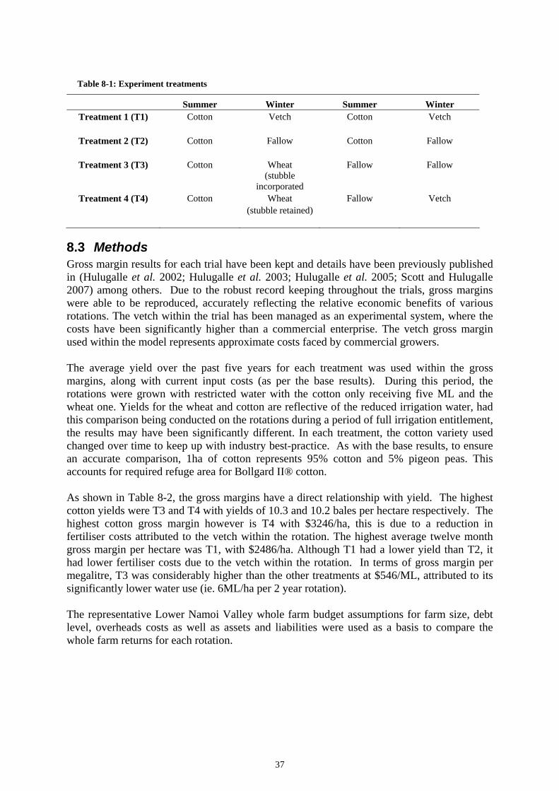
Table 8-1: Experiment treatments

Summer Winter Summer Winter Treatment 1 (T1) Cotton Vetch Cotton Vetch

Treatment 2 (T2) Cotton Fallow Cotton Fallow

Treatment 3 (T3) Cotton Wheat Fallow Fallow

(stubble

incorporated Treatment 4 (T4) Cotton Wheat Fallow Vetch

(stubble retained)

8.3 Methods Gross margin results for each trial have been kept and details have been previously published in (Hulugalle et al. 2002; Hulugalle et al. 2003; Hulugalle et al. 2005; Scott and Hulugalle 2007) among others. Due to the robust record keeping throughout the trials, gross margins were able to be reproduced, accurately reflecting the relative economic benefits of various rotations. The vetch within the trial has been managed as an experimental system, where the costs have been significantly higher than a commercial enterprise. The vetch gross margin used within the model represents approximate costs faced by commercial growers. The average yield over the past five years for each treatment was used within the gross margins, along with current input costs (as per the base results). During this period, the rotations were grown with restricted water with the cotton only receiving five ML and the wheat one. Yields for the wheat and cotton are reflective of the reduced irrigation water, had this comparison being conducted on the rotations during a period of full irrigation entitlement, the results may have been significantly different. In each treatment, the cotton variety used changed over time to keep up with industry best-practice. As with the base results, to ensure an accurate comparison, 1ha of cotton represents 95% cotton and 5% pigeon peas. This accounts for required refuge area for Bollgard II® cotton. As shown in Table 8-2, the gross margins have a direct relationship with yield. The highest cotton yields were T3 and T4 with yields of 10.3 and 10.2 bales per hectare respectively. The highest cotton gross margin however is T4 with $3246/ha, this is due to a reduction in fertiliser costs attributed to the vetch within the rotation. The highest average twelve month gross margin per hectare was T1, with $2486/ha. Although T1 had a lower yield than T2, it had lower fertiliser costs due to the vetch within the rotation. In terms of gross margin per megalitre, T3 was considerably higher than the other treatments at $546/ML, attributed to its significantly lower water use (ie. 6ML/ha per 2 year rotation). The representative Lower Namoi Valley whole farm budget assumptions for farm size, debt level, overheads costs as well as assets and liabilities were used as a basis to compare the whole farm returns for each rotation.

37

Table 8-2: Indicative Yields, Gross Margins and Water Use

Treatment Summer Winter Summer Winter 12 month

Treatment average

T1 Cotton Vetch Cotton Vetch

Yield 8.8 bales/ha - 8.8 bales/ha -

Gross Margin/ha $2656 -$170 $2656 -$170 $2486

ML/ha 5 1.4 5 1.4 6.4

Gross Margin/ML $531 -$121 $531 -$121 $388

T2 Cotton Fallow Cotton Fallow

Yield 8.9 bales/ha - 8.9 bales/ha -

Gross Margin $2503 -$47 $2503 -$47 $2456

ML/ha 5 - 5 - 5

Gross Margin/ML $501 - $501 - $491

T3 Cotton Wheat Fallow Fallow

Yield 10.3 bales/ha 2.7 t/ha - -

Gross Margin $3122 $366 -$179 -$31 $1639

ML/ha 5 1 - - 3

Gross Margin/ML $624 $366 - - $546

T4 Cotton Wheat Fallow Vetch

Yield 10.2 bales/ha 2.95 t/ha - -

Gross Margin $3246 $427 -$179 -$170 $1662

ML/ha 5 1 - 1.4 3.7

Gross Margin/ML $649 $428 - -$121 $449

To compare the rotations at a whole farm level, cropping area was determined by the scarcest resource (ie. irrigation water 1285ML). Land was allocated to each rotation to use all irrigation water, as each rotation used different amounts of water, the land allocated to each rotation varied (see Table 8-3). Two year rotations were compared by assuming the farm had two of the rotations active, in offset years (Table 8-4). This was particularly important for treatments 3 and 4 to ensure a twelve month snapshot captured the entire rotation.

Table 8-3: Land allocated to rotational crop

ML/ha Ha of rotation T1 12.8 100 T2 10 128 T3 6 214 T4 7.4 173

Table 8-4: Example of offset rotations

Summer Winter Summer Winter 12months 12 months

Treatment 1 (T1) Cotton (100ha) Vetch (100ha) Cotton (100ha) Vetch (100ha) T1 - offset Cotton (100ha) Vetch (100ha) Cotton (100ha) Vetch (100ha)

Treatment 4 (T4) Cotton (173ha) Wheat (173ha) Fallow (173ha) Vetch (173ha) T4 - offset Fallow (173ha) Vetch (173ha) Cotton (173ha Wheat (173ha)

By allocating land to the rotation in this way, it meant that in all of the rotations there would be a lot of unallocated land, unable to be irrigated due to the restricted water availability. As with the representative farm, dryland winter crops were allocated and 200ha per rotation was kept fallow (in addition to any fallow area already assumed to be within the rotation systems).

38

Gross Margins used for dryland crops and the cattle enterprise are as per the Lower Namoi Valley farm budget assumptions (Table 6-8).

8.4 Results of the rotations

8.4.1 Financial performance of individual rotations Utilising the above mentioned method for allocating area to the rotations, for each treatment within the whole farm comparison the area under crop can be seen in Table 8-5 to Table 8-8. The highest irrigation total gross margin was for T3 at $700,108, followed by T2 at $656,793. Sixteen percent lower than T3 was T4 at $587,719 and T1 was significantly lower than all the treatments at $534,211. Considering return per hectare from the 782 hectares of irrigation land available, this is equivalent to an annual gross margin of $683, $840, $895, $752/ha for treatments one through to four respectively. When considering the gross margin return from the 1285 megalitres of water available, this is equivalent to $416, $511, $545, $457/ha respectively.

Table 8-5: Area allocated to crop: Treatment 1

Ha Crop

Water Applie

d ML/ha

Total Water Use

(ML) GM/ ha

GM/ ML

TOTAL GM

T1: IRRIGATION (12 month) TOTALS: 1280 ML $ 683 $ 417 $ 534,211

200 BT Cotton (95% cotton, 5% pigeon peas) 5 1,000 $2,656 $ 531 $ 531,200

582 Summer Fallow (irrigated paddocks) 0 - -$ 79 - -$ 45,978

782 ha Summer Total 1,000 $ 485,222

200 Vetch 1.4 280 -$ 170 -$ 121 -$ 34,000

127 Dryland Wheat (on irrigation paddock with no irrigations) 0 - $ 188 - $ 23,876

127 Dryland Chickpea (on irrigation paddock with no irrigations) 0 - $ 336 - $ 42,672

127 Dryland Faba bean (on irrigation paddock with no irrigations) 0 - $ 226 - $ 28,702

201 Winter Fallow (irrigated paddocks) 0 - -$ 61 - -$ 12,261

782 ha Winter Total 280 $ 48,989 T1 (Table 8-5) had the lowest annual irrigation gross margin at $534,211. This treatment grew 200 hectares of cotton annually, which was the second lowest; this is due to 1.4 megalitres per hectare being allocated to Vetch within the rotation. Despite the inclusion of vetch into the rotation, T1 had the lowest cotton yields at 8.8 bales/ha. Whilst the rotation gross margin is the highest per hectare (Table 8-2), within this whole farm comparison both the return per hectare of $683 and the return per megalitre of $416 are lowest of all treatments. T2 (Table 8-6) grew the most cotton with 256 hectares allocated to the rotation. This is a result of the rotation being a monoculture, so water did not have to be allocated to any other crops. Whilst yields were approximately 13% lower compared to T3 and T4, resulting in gross margins being 25% lower, T2 returned the second highest annual gross margin of $840/ha (after T3 at $895/ha). Despite the lowest cotton gross margins, by growing 20, 28 and 47 percent more cotton than T3, T1 and T4, respectively, T2 was able to outperform T1

39

and T4 in terms of annual irrigation gross margin. This is attributed to all irrigation water used on the crop that returned the highest gross margin per megalitre.

Table 8-6: Area allocated to crop: Treatment 2

Ha Crop

Water Applied ML/ha

Total Water

Use GM/ha GM/ML TOTAL

GM

T2: IRRIGATION (12 month) TOTALS: 1280 ML $ 840 $ 513 $ 656,793

256 BT Cotton (95% cotton, 5% pigeon peas) 5 1,280 $2,503 $ 501 $ 640,768

526 Summer Fallow (irrigated paddocks) 0 - -$ 79 - -$ 41,554

782 ha Summer Total 1280 ML $ 599,214

256 Winter Fallow - Rotation 0 - -$ 47 - -$ 12,032

109 Dryland Wheat (on irrigation paddock with no irrigations) 0 - $ 188 - $ 20,492

109 Dryland Chickpea (on irrigation paddock with no irrigations) 0 - $ 336 - $ 36,624

109 Dryland Faba bean (on irrigation paddock with no irrigations) 0 - $ 226 - $ 24,634

199 Winter Fallow (irrigated paddocks) 0 - -$ 61 - -$ 12,139

782 ha Winter Total 0 ML $ 57,579

Table 8-7: Area allocated to crop: Treatment 3

Ha Crop

Water Applie

d ML/ha

Total Water

Use GM/ ha

GM/ ML

TOTAL GM

T3: IRRIGATION (12 month) TOTALS: 1285 ML $ 895 $ 545 $ 700,108

214 BT Cotton (95% cotton, 5% pigeon peas) 5 1,071 $3,122 $ 624 $ 668,628

214 Summer Fallow - rotation 0 - -$ 179 - -$ 38,336

354 Summer Fallow (irrigated paddocks) 0 - -$ 79 - -$ 27,940

782 ha Summer Total 1071 $ 602,353

214 Wheat - semi irrigated 1 214 $ 366 $ 366 $ 78,385

214 Winter Fallow - rotation 0 - -$ 31 - -$ 6,639

51 Dryland Wheat (on irrigation paddock with no irrigations) 0 - $ 188 - $ 9,588

51 Dryland Chickpea (on irrigation paddock with no irrigations) 0 - $ 336 - $ 17,136

51 Dryland Faba bean (on irrigation paddock with no irrigations) 0 - $ 226 - $ 11,526

201 Winter Fallow (irrigated paddocks) 0 - -$ 61 - -$ 12,241

782 ha Winter Total 214 ML $ 97,755 The second highest allocation to cotton with 214 hectares, T3 (Table 8-7) had the highest annual irrigation gross margin at $700,108. This can be attributed to this treatment achieving the highest cotton yields and the second highest cotton gross margin (marginally less than T4). Within this rotation wheat was grown, which gave a positive return of $366/ha. T4 (Table 8-8), had the second lowest annual irrigated gross margin at $587,719. This was 16% lower than T3. T4 had the smallest hectares allocated to the rotation at 173ha. This was

40

due to water being allocated to not only cotton, but also wheat and vetch. Although T3 and T4 both had the highest cotton gross margin per hectare, T4 performed significantly worse due to the reduction in hectares of cotton and also due to the cost of growing vetch within the rotation.

Table 8-8: Area allocated to crop: Treatment 4

Ha Crop

Water Applie

d ML/ha

Total Water

Use GM/ ha

GM/ ML

TOTAL GM

T4: IRRIGATION (12 month) TOTALS: 1280 ML $ 752 $ 459 $ 587,719

173 BT Cotton (95% cotton, 5% pigeon peas) 5 865 $3,246 $ 649 $ 561,558

173 Summer Fallow - rotation 0 - -$ 179 - -$ 30,967

436 Summer Fallow (irrigated paddocks) 0 - -$ 79 - -$ 34,444

782 ha Summer Total 865 $ 496,147

173 Wheat – semi irrigated 1 173 $ 427 $ 427 $ 73,871

173 Vetch 1.4 242 -$ 170 -$ 121 -$ 29,410

79 Dryland Wheat (on irrigation paddock with no irrigations) 0 - $ 188 - $ 14,852

79 Dryland Chickpea (on irrigation paddock with no irrigations) 0 - $ 336 - $ 26,544

79 Dryland Faba bean (on irrigation paddock with no irrigations) 0 - $ 226 - $ 17,854

199 Winter Fallow (irrigated paddocks) 0 - -$ 61 - -$ 12,139

782 ha Winter Total 415 ML $ 91,572

As the land was allocated to use all of the 1285 mega litres of irrigation water available, this resulted in each treatment having varying land allocated to the rotation (due to varying water use). This resulted in each treatments return per megalitre influencing the whole farm results. Had the comparison allocated equal hectares to each rotation, the results would have reflected profitability of the treatments as per Table 8-2. Other key factors in the performance between treatments, came down to area grown to cotton and cotton yields, as the financial performance of the farm is most sensitive to cotton (Figure 8.6). The importance of allocating water to non incoming generating crops like vetch is highlighted. Whilst the inclusion of vetch into a rotation may improve the overall gross margin per hectare, the gross margin per mega litre is significantly reduced.

8.4.2 Whole farm financial performance of cotton rotation study Within the steady state analysis, whole farm financial performance of the four treatments varied significantly, as displayed in Table 8-9. The irrigation income varied according to the crops grown and the area allocated to the rotation. Overheads common to all four treatments are consistent with the steady state analysis (Table 6-8), with the exception of casual labour which varied dependant on the hectares of crop grown. All other financial characteristics remained constant between the four treatments. Operating costs are also consistent with the steady state analysis (Table 6-8), with remuneration for the farm owner not included within this analysis. T2 and T3 have significantly reduced casual labour costs (as indicated in Table 8-9) this is due to these treatments growing considerably less green ha within the rotations.

41

Table 8-9: Financial Performance

Enterprise Gross Margins T1 T2 T3 T4

Irrigation 534,211 656,793 700,108 587,719

Dryland 31,295 31,295 31,295 31,295

Grazing 19,507 19,507 19,507 19,507

Total Farm Gross Margin: $585,013 $707,595 $750,910 $638,521

Overhead Costs

Common Overhead costs 151,066 151,066 151,066 151,066

Labour (variable depending on green ha's)

• Casual $20.00 /hr x FTE @ 55 hrs/week 35,094 4,211 3,951 31,195

Total Overhead Costs $186,160 $155,278 $155,018 $182,261

Net Farm Cash Income (Gross Margin less Overhead Costs) $398,853 $552,317 $595,892 $456,260

Operating Costs

Total Operating Costs 221,138 221,138 221,138 221,138

Farm Operating Surplus (Net Farm Cash Income less Operating Costs) $177,715 $331,180 $374,755 $235,122 %Return on total assets and operator labour (Operating Surplus/Total assets) 2.61% 4.86% 5.50% 3.45% %Return on equity and operator labour (Operating Surplus/Total equity) 3.57% 6.65% 7.52% 4.72% Farm operating surplus is an indication of a businesses ability to meet farm costs whilst maintaining assets (depreciation). The surplus was greatest for T3 and T2 at $374,755 and $331,180 respectively. T4 and T1 still returned surpluses, however these were significantly less than the other treatments at $235,122 and $177,715 respectively. T1’s operating surplus is just under half of T3’s. A positive farm operating surplus for all four treatments indicates that each rotation was able to meet farm costs and maintain assets. However, as debt repayments and owner living expenses need to taken from the farm operating surplus, it is evident that T3 and T2 are most likely to cope with these costs. The business return on equity ranged from 7.52% for T3 to 3.57% for T1. A business with a high return on equity has a greater capacity to generate funds within a business. This in turn gives the business a greater ability to repay debt and re-invest within the business.

8.4.3 Impact of price variability on cotton rotation study Similar to the steady state representative farm results, price variability has a significant impact on the different rotations. As the mean results were discussed and compared in the previous section (8.4.1 Financial performance of individual rotation), this section will compare the financial performance when price variability is taken into account. Each rotation is affected differently by the varying prices, depending on their reliance on particular commodity prices. The affect is depicted within a gross margin comparison in a box & whisker graph (Figure 8.1). The median result for each treatment is represented by the horizontal line in the middle of the box. The top of the box is the upper quartile with 75% of results occurring below these lines.

42

The bottom of the box represents the lower quartile with 25% of results occurring below these lines, the upper vertical lines end at the 95th percentile and the lower line ends at the 5th percentile with 5% of results occurring below this point. This particular box & whisker graph removes any outlying results by not reporting the top or bottom 5% or results.

Figure 8.1: Gross Margin comparison by treatment

Initially obvious is the shift of the data or the height of each box in comparison to the others. T1 is significantly lower than the other treatments and T3 is the highest. A lower placement of data indicates a probability of lower gross margin results. As seen in Table 8-10, T1 has a 48% probability of total gross margin under $500,000, whilst T3 has only an 6% likelihood of achieving a total gross margin under $500,000. Therefore the cotton-wheat rotation appears to be the most resilient to price variability. The spread or variability of the graphs is quite similar, each with short lower quartiles, similar length mid quartiles and all with longer upper quartiles. Each graph is skewed with the mean result lower than the median. This indicates that the gross margin results are most likely to be in the lower half of the range of results. Whilst the range of the results can suggest the size of risk. In this instance T2 & T3 have the widest range of potential gross margin results, however these ranges start higher and have topside potential (longer upper quartiles), indicating that there is opportunity to return significant gross margins.

Table 8-10: % Probability of Gross Margin result occurring below, above or between $500K and $700K

Treatment <$500,000 > < >$750,000 T1 48 44 8 T2 16 61 24 T3 6 62 31 T4 31 56 13

Net farm cash income comparison as displayed in Figure 8.2, indicates how much income remains once operating and overhead costs are covered. It is desirable for net farm cash income to be as high as possible to ensure that there are enough funds available to cover operating costs (including interest and depreciation), owner living expenses, debt repayments

43

or even re-investment in the business. There is an 81% probability that T1 will return a net farm cash income of under $500,000 whilst T3 has a 66% probability of returning a net farm cash income of over $500,000.

Figure 8.2: Net farm cash income comparison

Figure 8.3: Farm operating surplus comparison

Farm operating surplus (net farm cash income less operating costs of interest and depreciation) comparison is displayed in Figure 8.3. Normally this surplus would be used to fund principal loan repayments and the owners living expenses. All treatments are likely to

44

return an operating surplus. T3 is the most likely to achieve a positive surplus in excess of $500,000.

Figure 8.4: Return on assets comparison (%)

The treatment comparison of return on assets (operating surplus/total assets) shows how effective each treatment is at generating a profit for the business (Figure 8.4). All treatments are likely to return a positive return on assets, with T1 and T4 are most probably going to achieve a return on assets between 0 and 5%. T3 is the most likely to generate a significant profit with a 50% probability of achieving over 5% return. T2 closely follows with a 39% probability of achieving over 5% return on assets. The treatment comparison of return on equity (operating surplus/total equity) shows how much profit each treatment generates as a percentage of the business owners funds (or equity) (Figure 8.5). T1 and T4 are likely to generate a profit between 0 and 5%. T3 is the most likely to generate a significant profit with a 75% probability of achieving over 5%. T2 closely follows with a 38% probability of achieving over 5% return on equity.

45

Figure 8.5: Return on equity comparison (%)

To understand which variables have the greatest effect on profitability (net farm cash income), further sensitivity analysis was conducted. Figure 8.6 shows the results on how the profitability of the treatments vary with changes in specific variables, (in this case commodity prices including cotton lint, wheat, faba bean, chickpea, urea, anhydrous ammonia and diesel), while all other variables are held stable (at the mean). The tornado charts rank each input in terms of its impact on the profitability for each treatment. The variable with highest impact (indicated by the length of the bar) is at the top of the chart followed by other variables in descending impact order. The bar ends indicate the low and high value of the impact. In this comparison, the profitability of all treatments is most sensitive to the price of cotton lint. The analysis also indicates that the prices of the commodities being produced have more of an impact on profitability than the price of the various inputs such as fertiliser and fuel. In practice this means that the profitability of a farm is largely dependent on the price received for the commodities.

46

Figure 8.6: Sensitivity Charts (T1 to T4)

47

9. Conclusions

9.1 Representative farm This report presents a description of a representative farm in the Lower Namoi Valley and was developed and used to give a ‘snapshot’ of the financial performance of the model farm and to analyse the financial implications of changes in cropping rotations. The whole farm budget provides a snapshot of the financial performance at a particular point in time of a farm with a particular set of resources. The representative farm budget for the Lower Namoi Valley suggest that given restricted irrigation water availability and average commodity prices the business could return a profit. The $152,070 operating surplus indicates that after family living expenses minimal debt could be repaid in that twelve month period. If the business was to begin making off-farm investments, a considerably higher operating surplus would have to be achieved. The farm operating surplus achieved as a percentage of the owner’s equity is 3.1 per cent. The representative farm is resilient when it comes to poor commodity prices. Results suggest that in one year in five, the farm is unlikely to return a positive cash surplus due to pricing fluctuations. As the farm is 99% likely to return positive net farm cash income, this suggests that the debt levels assumed may be too high for the income earning capacity of the business, during sustained periods of low water allocation. This is also given the assumed commodity prices as listed in Chapter 6. Improvement in the cotton price as a result of better farm marketing strategies or improving world prices would make a significant difference to farm profitability. Recent trends in crop selection have seen farmers moving away from fixed rotations and making planting decision based on commodity values. This ability to adapt crop selection should increase the long term profitability of the typical farming system providing soil health is not compromised and best practice agronomy is adhered to.

9.2 Whole farm impacts of rotations and tillage The whole farm comparison snapshot of the four cotton based rotation trials, highlights the importance of crop selection in terms of financial performance. Mean results indicated a positive return for all rotations within the representative farm budgets for the Lower Namoi Valley. Farm operating surplus ranged from $177,715 to $374,755 indicating that in restricted irrigation water availability scenarios, assuming average commodity prices, each rotation would generate a profit. The two year rotation of cotton, wheat, followed by summer and winter fallows was the treatment able to generate the highest business return. The same rotation was most resilient to commodity price variability, 100% likely to return a positive farm operating surplus and 20% likely to return over $500,000. The two rotations including vetch were the least resilient to variable commodity prices. As land was allocated to use all of the irrigation water available, each treatment’s return per megalitre influenced the whole farm results. The use of irrigation water on a non income crop (in this case vetch), reduced the rotations return per megalitre. Had the comparison allocated equal hectares to each rotation, the results would have reflected the profitability of the treatments as per Table 8-2.

48

This analysis assumed restricted availability of irrigation water. During periods of increased water availability, the wheat crop would receive more irrigation applications to increase yield which would positively affect the gross margins of those treatments. The development of the whole-farm model described in this Report has been profitability focused. It is important to note the other considerations of crop selection which affect the long term sustainability of the irrigation farming business. Science has proven the numerous benefits of including various crops in rotation with cotton from management of pests, weeds and disease through to improved soil nutrition and structure. A budget snapshot does not take into account these agronomic benefits.

49

10. References ABARE (1997). Effect of interest rate changes on farm sector incomes, ABARE Current

Issues. Australian Bureau of Agricultural and Research Economics, Canberra.

ABARE (2008). Cotton, Australian Commodity Statistics 2008. http://www.abareconomics.com/interactive/08acs_dec/excel/Cotton.xls.

ABARE (2008). Farm Inputs, Australian Commodity Statistics 2008. http://www.abareconomics.com/interactive/08acs_dec/excel/Cotton.xls.

ABS (2008). Agricultural Commodities: Small Area Data, Australia, 2005-06 (Reissue). Catalogue 7125.0. Australian Bureau of Statistics, Canberra.

ABS (2008). Agricultural Commodities: Small Area Data, Australia, 2006-07. Catalogue 7125.0. Australian Bureau of Statistics, Canberra.

ABS (2008). Water Use on Australian Farms, 2005-06 (Additional Datacubes). Catalogue 4618.0. Australian Bureau of Statistics, Canberra.

ABS (2008). Water Use on Australian Farms, 2006-07. Australian Bureau of Statistics, Canberra.

ABS (2009). Water Use on Australian Farms, 2007-08 (Additional Datacubes). Catalogue 4618.0. Australian Bureau of Statistics, Canberra.

AIP (2009). Retail Diesel Price - Weekly Average - NSW Regional Average. Australian Institute of Petroleum, Canberra.

Ali, M.H., Hoque, M.R., Hassan, A.A. and Khair, A. (2007). Effects of deficit irrigation on yield, water productivity, and economic returns of wheat, Agricultural Water Management 92: 151-161.

ANRA (2009). Water resources - Overview - New South Wales - Namoi River. Australian Natural Resources Atlas.

ANZ (2009). Import Parity Price Series. Australia and New Zealand Banking Group Limited, Melbourne.

Ashton, D. and Oliver, M. (2008). An Economic Survey of Irrigation Farms in the Muray-Darling Basin: Industry overview and region profiles, Canberra.

Baillie, J., Baillie, C., Heinrich, N. and Murray, A. (2008). On-farm water use efficiency in the Northern Murray-Darling Basin. Murray Darling Basin Commission - Northern Basin Program, Canberra.

Bennett, R., Kambhampati, U., Morse, S. and Ismael, Y. Farm-level economic performance of genetically modified cotton in Maharashtra, India, Review of Agricultural Economics (Boston). 2006. 28: 1, 59-71. 22 ref.

50

Blackburn, A. and Ashby, R. (2007). Financing Your Farm: A practical guide to financial growth. Australian Bankers' Association Inc.

BOM (2009). Climate Statistics for Australian Locations. Australian Bureau of Meteorology, Canberra.

Boyce & Co (2006). Australian Cotton Comparative Analysis. Boyce Charted Accountants, Moree.

Cotton Australia (2004). Annual Report 2003/2004. Cotton Australia, Sydney.

Cotton Australia (2005). Annual Report 2004/2005. Cotton Australia, Sydney.

Cotton Australia (2006). Annual Report 2005/2006. Cotton Australia, Sydney.

Cotton Australia (2007). Annual Report 2006/2007. Cotton Australia, Sydney.

Cotton Australia (2008). Annual Report 2007/2008. Cotton Australia, Sydney.

Cotton Australia (2008). Growers Toolkit - Best Managment Practices. http://www.cottonaustralia.com.au/toolkit/bmp/, Viewed14-10-2008.

Cotton Australia (2009). Annual Report 2008/2009. Cotton Australia, Sydney.

Cotton Consultants Australia (2008). Post Season Survey 2007/2008. Western Research Institute, Narrabri.

Cotton CRC (2008). Reducing Fertiliser Costs with Vetch, Healthy Soils Case Study. Cotton Catchment Communities CRC, Narrabri.

Cotton CRC and CRDC (2009). Rotation Crops and Cotton. Cotton Catchment Communities CRC, Narrabri.

Cox, H., Kelly, R. and Strong, W. (2010). Forthcoming article 'Pulse crops in rotation with cereals are a profitable alternative to nitrogen fertiliser in central Queensland', Crop and Pasture Science.

Crean, J. (2001). Database of Regulated Surface Water Licenses - Namoi Valley. Unpublished.

CSIRO (2006). Climate Change in the Namoi Catchment. CSIRO.

Donaldson, S. and Heath, T. (1997). Namoi River Catchment: Report on land degradation & proposals for integrated management. DLWC, Gunnedah.

DWE (2009). Water Access Licence Statistics. Department of Water & Energy.

Hope, M. and Bennett, R. (2002). Namoi Catchment Irrigation Profile. Report prepared for Water Use Efficiency Advisory Unit, Dubbo.

Hulugalle, N. and Scott, J.F. (2008). A review of the changes in soil quality and profitability accomplished by sowing rotation crops after cotton in Australian Vertosols from 1970 to 2006, Australian Journal of Soil Research 46: 173-190.

51

Hulugalle, N., Weaver, T. and Scott, J. (2008). Final Report: Maintaining profitability and soil quality in cotton farming systems II. Cotton Catchment Communities CRC.

Hoogmoed, W. (ed.)^(eds.) (Year). Soil organic carbon and profitability of irrigated cotton sown into standing wheat stubble., Proceedings of the Proceedings 16th Triennial Conference of the International Soil Tillage Research Organisation (ISTRO); 13-18 July 2003 Brisbane, Qld.

Hulugalle, N.R., Entwistle, P.C., Weaver, T.B., Scott, J.F. and Finlay, L.A. (2002). Cotton-based rotation systems on a sodic Vertosol under irrigation: effects on soil quality and profitability, Australian Journal of Experimental Agriculture 42: 341-349.

Hulugalle, N.R., Weaver, T.B. and Scott, F. (2005). Continuous cotton and cotton-wheat rotation effects on soil properties and profitability in an irrigated vertisol, Journal of Sustainable Agriculture 27: 5-24.

Isbell, R.F. (1996). The Australian Soil Classification. CSIRO Publishing Melbourne.

Levine, D., Stephan, D., Krehbiel, T. and Berenson, M. (2005). Statistics for Managers Using Microsoft Excel. Pearson Eduction Inc., Upper Saddle River.

Malcolm, B., Makeham, J. and Wright, V. (2005). The Farming Game, Agricultural Management and Marketing. Cambridge University Press, New York.

Marcellos, H. and Felton, W.L. (1992). Cropping systems of the temperate summer rainfall region, 6th Annual Australian Society of Agronomy Conference.

Namoi CMA. Namoi Catchment Management Authority Area Map. http://www.namoi.cma.nsw.gov.au/21.html?1.

Palisade (2009). Guide to Using @RISK. Palisade Corporation, Ithaca.

Payero, J. and Harris, G. (2008). Optimising Irrigated Grain Production with Limited Water. Grains Research & Development Corportation, http://www.grdc.com.au/director/research/standards.

Powell, J. (2009). A timeseries of the Australian cotton industry. Cotton Catchment Communities CRC, Narrabri.

Pulse Australia (2009). General Crop Information. Pulse Australia.

RBA (2009). Daily Exchange Rates of the Australian Dollar. Reserve Bank of Australia, Canberra.

Rochester, I. (2004). Vetch - the legume that increases cotton profits. CSIRO Plant Industry, Narrabri.

Rochester, I. and Peoples, M. (2005). Growing vetches (Vicia villosa Roth) in irrigated cotton systems: inputs of fixed N, N fertiliser savings and cotton productivity, Plant and Soil. 2005. 271: 1/2, 251-264. many ref.

Roth, G. (2006). Towards Sustainable and Profitable Water Use in the Australian Cotton Industry. Cotton Catchment Communities CRC, Narrabri.

52

53

Scott, J.F. and Hulugalle, N. (2007). Rotations and permanent beds to fight the cotton cost-price squeeze, Australian Cottongrower 28: 41-45.

The Australian Cotton Grower (2003). Cotton Yearbook 2003, The Australian Cotton Grower. Greenmount Press, Toowoomba.

The Australian Cotton Grower (2004). Cotton Yearbook 2004, The Australian Cotton Grower. Greenmount Press, Toowoomba.

The Australian Cotton Grower (2005). Cotton Yearbook 2005, The Australian Cotton Grower. Greenmount Press, Toowoomba.

The Australian Cotton Grower (2006). Cotton Yearbook 2006, The Australian Cotton Grower. Greenmount Press, Toowoomba.

The Australian Cotton Grower (2007). Cotton Yearbook 2007, The Australian Cotton Grower. Greenmount Press, Toowoomba.

The Australian Cotton Grower (2008). Cotton Yearbook 2008, The Australian Cotton Grower. Greenmount Press, Toowoomba.

Tulloh, C., Ahammad, H., Mi, R. and Ford, M. (2009). Effect of the Carbon Pollution Reduction Scheme on the economic value of farm production, Issues insights. Australian Bureau of Agricultural and Research Economics, Canberra.

USDA (2009). Table 9: World Cotton Supply and Distribution, http://www.fas.usda.gov/psdonline/. United States Department of Agriculture, Foreign Agricultural Service, 10/06/2009.

11. Appendix A: Distribution graphs @Risk distribution graphs as discussed in section 6.2 Commodity Prices

Figure 11.1: Cotton lint price distribution

Cotton lint ($/bale)

616.5372.75.0%90.0%5.0%

0

0.001

0.002

0.003

0.004

0.005

0.006

0.007

0.008

300

350

400

450

500

550

600

650

700

750

Values in $

InvGauss(137.51,383.49,RiskTruncate(0,500),RiskShift(325))

Figure 11.2: Cotton seed price distribution

Cotton seed ($/t)

146.0 360.55.0% 90.0% 5.0%

0

0.001

0.002

0.003

0.004

0.005

0.006

50 100

150

200

250

300

350

400

450

500

Values in $

Pert(100,234,450)

Figure 11.3: Chickpea price distribution

Chickpea ($/t)

703272 5.0%90.0%5.0%

0

0.0005

0.001

0.0015

0.002

0.0025

0.003

200

300

400

500

600

700

800

Values in $

BetaGeneral(1.3094,1.8922,239.06,798.67,RiskTruncate(241,788))

Figure 11.4: Wheat price distribution

Wheat ($/t)

402.9181.75.0%90.0%5.0%

0

0.002

0.004

0.006

0.008

0.01

0.012

0.014

0.016

150

200

250

300

350

400

450

500

Values in $

InvGauss(79.663,59.023,RiskTruncate(0,450),RiskShift(170))

54

Figure 11.5: Faba bean price distribution

Faba bean ($/t)

584202 5.0%90.0%5.0%

0

0.0005

0.001

0.0015

0.002

0.0025

0.003

0.0035

0.004

0.0045

100

200

300

400

500

600

700

800

Values in $

LogLogistic(90.808,233.71,3.507,RiskTruncate(168,800))

Figure 11.6: Maize price distribution

Maize ($/t)

455.8181.55.0%90.0%5.0%

0

0.001

0.002

0.003

0.004

0.005

0.006

150

200

250

300

350

400

450

500

550

600

650

Values in $

Weibull(1.4135,135.31,RiskTruncate(0,480),RiskShift(165))

Figure 11.7: Sorghum price distribution

Sorghum ($/t)

373.4167.15.0%90.0%5.0%

0

0.001

0.002

0.003

0.004

0.005

0.006

0.007

0.008

0.009

150

200

250

300

350

400

450

500

Values in $

InvGauss(143.04,599.35,RiskTruncate(68,600),RiskShift(91.135))

Figure 11.8: Anhydrous Ammonia price distribution

Anydrous Ammonia ($/t)

1.5880.9065.0%90.0%5.0%

0

0.000005

0.00001

0.000015

0.00002

0.000025

0.00003

0.000035

0.8 1

1.2

1.4

1.6

1.8 2

Values in Thousands

InvGauss(307.68,388.27,RiskTruncate(0,1160),RiskShift(840))

55

Figure 11.9: Di-Ammonium Phosphate (DAP) price distribution

Figure 11.11: Diesel price distribution

Diesel (¢/L)

179.0119.35.0%90.0%5.0%

0

0.005

0.01

0.015

0.02

0.025

80 100

120

140

160

180

200

220

Values in $

ExtValue(136,15.2,RiskTruncate(100,210))

DAP ($/t)

1.3640.4805.0%90.0%5.0%

0

0.000005

0.00001

0.000015

0.00002

0.000025

0.00003

0.000035

0.00004

0.000045

0.00005

0.4

0.6

0.8 1

1.2

1.4

1.6

1.8

Values in Thousands

Pearson5(0.946,119,RiskTruncate(0,1440),RiskShift(440))

Figure 11.10: Urea price distribution

Urea ($/t)

0.8300.4335.0%90.0%5.0%

0

0.00001

0.00002

0.00003

0.00004

0.00005

0.00006

0.00007

0.4

0.5

0.6

0.7

0.8

0.9 1

1.1

Values in Thousands

InvGauss(157.55,166.21,RiskTruncate(0,800),RiskShift(403.28))

12. Appendix B: Commodity Correlations

Table 12-1: Grain and legume price correlations

Hard Wheat

11.5 ESR Chickpea Maize Faba bean Sorghum

Hard Wheat 11.5 ESR 1.00 Chickpea 0.22 1.00 Maize 0.36 0.60 1.00 Faba bean 0.55 0.45 0.80 1.00 Sorghum 0.29 0.60 0.89 0.69 1.00

56

Table 12-2: Fertiliser and diesel price correlations

Urea AA DAP Diesel

Urea 1.00 AA 0.75 1.00 DAP 0.89 0.78 1.00

Diesel 0.83 0.73 0.88 1.00

57

13. Appendix C: Plant & Equipment Register

PLANT & EQUIPMENT REGISTER

Item Market Salvage

Value Value

Tractor 1 JD 6230 - 57 KW PTO (76 HP) AND 70 KW ENGINE (95 HP) $60,824 $21,288

Tractor2 JD 6230 - 57 KW PTO (76 HP) AND 70 KW ENGINE (95 HP) $60,824 $21,288

Tractor 3 JD 8230 - 149 KW PTO (200 HP) AND 177 KW ENGINE (240 HP) $178,875 $62,606

Tractor 4 JD 8430 - 186 KW PTO (250 HP) AND 217 KW ENGINE (295 HP) $235,146 $82,301

Machine 1 4WD ute $28,000 $16,800

Machine 2 4WD ute $28,000 $16,800

Machine 3 Landcruiser ute $56,990 $34,194

Machine 4 Back hoe $15,000 $9,000

Machine 5 Roberville Auger $15,000 $9,000

Machine 6 Semi tipper $25,000 $15,000

Machine 7 Min-till Air seeder+harrows: 12.2m width: 10km/ha: 8.54ha/hr $152,000 $91,200

Machine 8 Spray unit: 24m width: 18km/ha: 36.72ha/hr $38,000 $22,800

Machine 9 Cultivator: 8m width: 12km/ha: 8.64ha/hr $29,000 $17,400

Machine 10Mulcher with root cutters:8m width: 15km/ha: 5.1ha/hr $54,000 $32,400

Machine 11Interrow cultivator: 8m width: 9km/ha: 6.48ha/hr $35,000 $21,000

Machine 12Middle busting rig: 8m width: 6km/ha: 4.32ha/hr $30,000 $18,000

Machine 13Planter: 8m width: 10km/ha: 7.2ha/hr $59,000 $35,400

Machine 14Shielded spray rig: 8m width: 15km/ha: 10.8ha/hr $11,000 $6,600

Machine 15Spray unit: 18.2m width: 12km/ha: 18.564ha/hr $19,000 $11,400

Machine 16Bed renovator: 8m width: 6km/ha: 3.84ha/hr $34,000 $20,400

Workshop Contents of workshop $30,000 $4,000

Total $1,194,659 $568,878

58

14. NSW Department of Industry and Investment Economic Research Report Series

All available at http://www.dpi.nsw.gov.au/research/areas/biosecurity/economics-research/reports

Number 1 Brennan, J.P. and Bantilan, M.C.S. (1999), Impact of ICRISAT Research on Australian

Agriculture, Report prepared for Australian Centre for International Agricultural Research, Economic Research Report No. 1, NSW Agriculture, Wagga Wagga.

2 Davies, B.L., Alford, A. and Hollis, G. (1999), Analysis of ABARE Dairy Data for Six

Regions in NSW 1991-92 to 1996-97, Economic Research Report No 2, NSW Agriculture, C.B. Alexander College, Paterson.

3 Brennan, J.P. and Singh, R.P. (2000), Economic Assessment of Improving Nutritional

Characteristics of Feed Grains, Report prepared for Grains Research and Development Corporation, Economic Research Report No. 3, Wagga Wagga.

4 Zhao. X., Mullen, J.D., Griffith, G.R., Griffiths, W.E. and Piggott, R.R. (2000), An

Equilibrium Displacement Model of the Australian Beef Industry, Economic Research Report No 4, NSW Agriculture, Armidale.

5 Griffith, G., I’Anson, K., Hill, D., Lubett, R. and Vere, D. (2001). Previous Demand

Elasticity Estimates for Australian Meat Products, Economic Research Report No 5, NSW Agriculture, Armidale.

6 Griffith, G., I’Anson, K., Hill, D. and Vere, D. (2001). Previous Supply Elasticity

Estimates for Australian Broadacre Agriculture, Economic Research Report No 6, NSW Agriculture, Armidale.

7 Patton, D.A. and Mullen, J.D. (2001), Farming Systems in the Central West of NSW: An

Economic Analysis, Economic Research Report No. 7, NSW Agriculture, Trangie. 8 Brennan, J.P. and Bialowas, A. (2001), Changes in Characteristics of NSW Wheat

Varieties, 1965-1997, Economic Research Report No. 8, NSW Agriculture, Wagga Wagga.

9 Mullen, J.D. (2001), An Economic Perspective on Land Degradation Issues, Economic

Research Report No. 9, NSW Agriculture, Orange. 10 Singh, R.P., Mullen, J.D., and Jayasuriya, R. (2005), Farming Systems in the

Murrumbidgee Irrigation Area in NSW: An Economic Analysis, Economic Research Report No. 10, NSW Department of Primary Industries, Yanco.

11 Brennan, J.P., Aw-Hassan, A., Quade, K.J. and Nordblom, T.L. (2002), Impact of

ICARDA Research on Australian Agriculture, Economic Research Report No. 11, NSW Agriculture, Wagga Wagga.

59

12 Alford, A., Griffith, G. and Davies, L. (2003), Livestock Farming Systems in the

Northern Tablelands of NSW: An Economic Analysis, Economic Research Report No. 12, NSW Agriculture, Armidale.

13 Alford, A., Griffith, G. and Cacho, O. (2003), A Northern Tablelands Whole-Farm

Linear Program for Economic Evaluation of New Technologies at the Farm Level, Economic Research Report No. 13, NSW Agriculture, Armidale.

14 Mullen, J.D. and Vere, D.T. (2003), Research and Extension Capabilities - Program

Economists in New South Wales Agriculture, Economic Research Report No. 14, NSW Agriculture, Orange.

15 Farquharson, R.J., Griffith, G.R., Barwick, S.A., Banks, R.G. and Holmes, W.E. (2003),

Estimating the Returns from Past Investment into Beef Cattle Genetic Technologies in Australia, Economic Research Report No. 15, NSW Agriculture, Armidale.

16 O'Donnell, C.J., Griffith, G.R., Nightingale, J.J. and Piggott, R.R. (2004), Testing for

Market Power in Multiple-Input, Multiple-Output Industries: The Australian Grains and Oilseeds Industries, Technical Report for the Rural Industries Research and Development Corporation, Economic Research Report No. 16, NSW Agriculture, Armidale.

17 Brennan, J.P., Martin, P.J. and Mullen, J.D. (2004), An Assessment of the Economic,

Environmental and Social Impacts of NSW Agriculture’s Wheat Breeding Program, Economic Research Report No. 17, NSW Agriculture, Wagga Wagga.

18 Griffith, G.R., Davies, B.L., Alford, A.R., Herd, R.M., Parnell, P.F. and Hegarty, R.S.

(2004), An Assessment of the Economic, Environmental and Social Impacts of NSW Agriculture’s Investment in the Net Feed Efficiency R,D&E Cluster, Economic Research Report No. 18, NSW Department of Primary Industries, Armidale.

19 Scott, J.F. and Farquharson, R.J. (2004), An Assessment of the Economic Impacts of

NSW Agriculture’s Research and Extension: Conservation Farming and Reduced Tillage in Northern NSW, Economic Research Report No. 19, NSW Department of Primary Industries, Tamworth.

20 Scott, J.F., Farquharson, R.J. and Mullen, J.D. (2004), Farming Systems in the Northern

Cropping Region of NSW: An Economic Analysis, Economic Research Report No. 20, NSW Department of Primary Industries, Tamworth.

21 Crean, J., Shaw, A., Singh. R. and Mullen, J.D. (2004), An Assessment of the

Economic, Environmental and Social Impacts of NSW Agriculture’s Advisory Programs in Water Use Efficiency, Economic Research Report No. 21, NSW Department of Primary Industries, Orange.

22 Mullen, J.D. (2004), Evaluations in 2003 of Five Areas of Investment by NSW

Agriculture: Summary, Economic Research Report No. 22, NSW Department of Primary Industries, Orange.

60

23 Vere, D.T., Jones, R.E. and Dowling, P.M. (2004), An Economic Evaluation of Research into the Improved Management of the Annual Grass Weed Vulpia in Temperate Pastures in South-Eastern Australia, Economic Research Report No. 23, NSW Department of Primary Industries, Orange.

24 Jones, R.E. and Dowling, P.M. (2004), Sustainability, Externalities and Economics: The

Case of Temperate Perennial Grazing Systems in NSW, Economic Research Report No. 24, NSW Department of Primary Industries, Orange.

25 Brennan, J.P. and Quade, K.J. (2004), Analysis of the Impact of CIMMYT Research on

the Australian Wheat Industry, Economic Research Report No. 25, NSW Department of Primary Industries, Wagga Wagga.

26 Brennan, J.P., Sykes, J.D. and Scott, J.F. (2005), Trends in Pulse and Oilseed Crops in

Winter Cereal Rotations in NSW, Economic Research Report No. 26, NSW Department of Primary Industries, Wagga Wagga.

27 Vere, D.T., Griffith, G.R. and Silvester, L. (2005), Australian Sheep Industry CRC:

Economic Evaluations of Scientific Research Programs, Economic Research Report No. 27, NSW Department of Primary Industries, Orange.

28 Singh, R.P., Brennan, J.P. Lacy, J. and Steel, F. (2005), An Assessment of the Economic,

Environmental and Social Impacts of the Ricecheck Program, Economic Research Report No. 28, NSW Department of Primary Industries, Yanco.

29 Jones, R., Saunders, G. and Balogh, S. (2005), An Economic Evaluation of a Pest

Management Control Program: “Outfox the Fox”, Economic Research Report No. 29, NSW Department of Primary Industries, Orange.

30 Griffith, G.R., Parnell, P.F. and McKiernan, W. (2005), An Evaluation of the Economic

Benefits to NSW from Investment in the CRC for Beef Genetics Technologies, Economic Research Report No. 30, NSW Department of Primary Industries, Orange.

31 Khairo, S.A., Mullen, J.D., Hacker, R.B. and Patton, D.P (2006), Farming Systems in

the Western Division of NSW: An economic Analysis, Economic Research Report No. 31, NSW Department of Primary Industries, Trangie.

32 Griffith, G., Vere, D., and Jones, R. (2006), Sheep CRC Renewal Proposal:Economic

Evaluation of the Proposed Scientific Themes, Economic Research Report No. 32, NSW Department of Primary Industries, Armidale.

33 Alford, A.R., Cafe, L.M., Greenwood, P.L. and Griffith, G.R. (2007), The Economic

Effects of Early-Life Nutrition in Crossbred Cattle Bred on the NSW North Coast, Economic Research Report No. 33, NSW Department of Primary Industries, Armidale.

34 Jones, R. and Aluwihare, P. (2007), A bioeconomic model for measuring the opportunity

costs of water sharing plans in unregulated river systems: the Mooki river catchment, Economic Research Report No. 34, NSW Department of Primary Industries, Orange.

61

35 Davies, B.L., Carberry, P.M., Graham, R.P., Mullen, J.D. and Meaker, G.P., (2007) StockPlan®: A Decision Aid for Management of Livestock During Drought and Other Times, Economic Research Report No. 35, NSW Department of Primary Industries, Paterson.

36 Gibson, T.S., Allan, G.L., File, G., Mullen, J.D., Scott-Orr, H., 2005, ‘Priorities and

Principles for Investment in Aquaculture Research by NSW Department of Primary Industries’, Economic Research Report No. 36, NSW Department of Primary Industries, Orange.

37 Mounter, S., Griffith, G., Piggott, R., Fleming, E. and Zhao, X. (2007), Composition of

the National Sheep Flock and Specification of Equilibrium Prices and Quantities for the Australian Sheep and Wool Industries, 2002-03 to 2004-05, Economic Research Report No. 37, NSW Department of Primary Industries, Armidale, September.

38 Mounter, S., Griffith, G., Piggott, R., Fleming, E. and Zhao, X. (2007), An Equilibrium

Displacement Model of the Australian Sheep and Wool Industries, Economic Research Report No. 38, NSW Department of Primary Industries, Armidale, September.

39 Davies, L., Quinn, H., Della Bosca, A., Griffith, G., Trengove, G. and Alford, A. (2007),

The Economic Effects of Alternate Growth Path and Breed Type Combinations to Meet Beef Market Specifications across Southern Australia, Economic Research Report No. 39, NSW Department of Primary Industries, Armidale, September.

40 Orr, L., McDougall, S. and Mullen, J. (2008), An Evaluation of the Economic,

Environmental and Social Impacts of NSW DPI Investments in IPM Research in Lettuce, Economic Research Report No. 40, NSW Department of Primary Industries, Orange.

41 Orr, L., Stevens, M. and Mullen, J. (2008), An Evaluation of the Economic,

Environmental and Social Impacts of NSW DPI Investments in IPM Research in Invertebrate Rice Pests, Economic Research Report No. 41, NSW Department of Primary Industries, Orange.

42 Alford, A.R., McKiernan, W.A., Cafe, L.M., Greenwood, P.L. and Griffith, G.R. (2008),

The Economic Effects of Using Heterozygotes for a Non-functional Myostatin Mutation within a Commercial Beef Production System, Economic Research Report No. 42, NSW Department of Primary Industries, Armidale, May.

43 Nordblom, T.L., Finlayson, J.D., Hume, I.H., and Kelly, J.A. (2009, rev May 2010),

Supply and Demand for Water use by New Forest Plantations: a market to balance increasing upstream water use with downstream community, industry and environmental use? Economic Research Report No 43, NSW Department of Primary Industries, Wagga Wagga.

44 Alford, A.R., Garcia, S.C., Farina, S. and Fulkerson, W.J. (2009), An Economic

Evaluation of the Future Dairy Complementary Forage Rotation System – Using Cost Budgeting. Economic Research Report No. 44, 13. Industry & Investment NSW, Armidale, August

62

63

45 Alford, A.R., Garcia, S.C., Farina, S. and Fulkerson, W.J. (2009), An Economic Evaluation of the Future Dairy Complementary Forage Rotation System – Using Whole Farm Budgeting. Economic Research Report No. 45, Industry & Investment NSW, Armidale, August.

46 Powell, J. and Scott, F. (2011), A Representative Irrigated Farming System in the Lower

Namoi Valley of NSW: An Economic Analysis. Economic Research Report No. 46, Industry & Investment NSW, Narrabri, January.