Ad Hoc Networks 123 (2021) 102643

A1

Contents lists available at ScienceDirect

Ad Hoc Networks

journal homepage: www.elsevier.com/locate/adhoc

A reliable deep learning-based algorithm design for IoT load identification insmart gridYanmei Jiang a,d, Mingsheng Liu a, Hao Peng b,∗, Md Zakirul Alam Bhuiyan c

a State Key Laboratory of Reliability and Intelligence of Electrical Equipment, Hebei University of Technology, Tianjin, 300130, Chinab School of Cyber Science and Technology, Beihang University, Beijing, 100083, Chinac Department of Computer and Information Sciences, Fordham University, NY, 10458, USAd Department of Rail Transportation, Hebei Jiaotong Vocational and Technical College, Shijiazhuang, 050035, China

A R T I C L E I N F O

Keywords:Deep convolution neural networkFeature discriminationLoad identificationLong short-term memory networkNon-intrusiveTime-frequency transformation

A B S T R A C T

In IoT load monitoring system of the smart grid, the non-intrusive load monitoring and identification (NILMI)has become the research focus. However, the existing researches focus on the accuracy of load identification,neglecting the effectiveness of data sampled, the distinction of load abstract feature representation, and thereliability of load identification model. This paper proposes a novel algorithm framework of spatial–temporalconvolution neural network for NILMI, namely DST-CNN, to realize the fine-grained load identification. Inthe DST-CNN framework, to ensure the accuracy and reliability of data usage, an signal enhancement method,AM-PCA, is used. To enhance the distinction of load abstract feature representation, an extraction mechanism ofthe spatial–temporal features is developed, which utilizes deep convolution networks and time-series recurrentneural networks (RNN). To improve the accuracy and reliability of load identification model, a hierarchicalload classification mechanism is constructed, and the deep long short–term memory (LSTM) structure as theclassifier. A considerable amount of the high-frequent current signals are sampled to validation the performanceof the proposed method. The experimental results demonstrate the good generalization performance andsuperiority for NILMI in IoT load monitoring system.

1. Introduction

With the rapid development of Internet technology, IoT technologyis widely used in the smart grid. In the IoT load monitoring system,NILMI is a critical part of the load-side management of the ubiquitoussmart grid [1]. It could not only help enhance the operational efficiencyof the power grid side, but can alleviate the energy pressure, andimprove energy efficiency [2,3]. Especially, monitoring the current,voltage and the power of the device can effectively analyze the powerconsumption, the running situation of equipment, and the electricityusage of people [4–7]. However, most of the existing approaches forNILMI still need to be improved: the generalization of load identifica-tion model, the accuracy and reliability of load identification, and thedistinction of load abstract feature representation. These can inhibit theperformance or impact the reliability of the NILMI. In this article, ourstudy mainly includes: improving the validity of load data sampled,the capability of load characteristic representation, and the accuracyof the fine-grained load identification without overlay scene. It is veryimportant for improving the dependability of IoT load monitoringsystem in smart grid [8,9].

∗ Corresponding author.E-mail address: penghao@buaa.edu.cn (H. Peng).

A substantial amount of methods for NILMI have be presented inthe literature. These methods can be divided into two categories: themathematical optimization and the data driving [10,11]. The formerone is to solve the minimum of the combination results, namely thedifference is between the total power of the equipment combinationand the target loads value of a given set of equipment, and then in thecombination, the equipment included is the identification result. Themost of algorithms include the maximum likelihood function, the meanvalue and variance based on statistical characteristics, etc [12,13]. Inthe past few years, these methods have presented competitive perfor-mance for NILMI, however, there are still some shortcomings: relyingon a great deal of prior knowledge; a huge amount of computationsare required to determine the model parameters; the early models havesome serious limitations, which can affect the reliability of IoT loadmonitoring system [14].

In the present stage, the data-driven methods include DecisionTrees, k-Nearest Neighbor (kNN), Hidden Markov Models (HMM), andRandom Forest (RF), etc, which have the distinct advantages over theprevious methods of NILMI [15,16]. However, these methods require a

vailable online 8 August 2021570-8705/© 2021 Elsevier B.V. All rights reserved.

https://doi.org/10.1016/j.adhoc.2021.102643Received 27 March 2021; Received in revised form 20 June 2021; Accepted 30 Jul

y 2021

Ad Hoc Networks 123 (2021) 102643Y. Jiang et al.

sr

2

sfttdaolt

large number of offline data sets to train model; the parameter valuesneed to be adjusted frequently and to identify the best model, whichwill increase the computational burden of the algorithm.

Recently, in view of the excellent feature representation ability,the deep learning has been quickly applied in NILMI. In [17], theauthor uses the convolution neural network (CNN) to extract the loadfeatures of the different appliances in NILMI. In [18], the Bayesiannon-parametric learning-based approach and long short–term memory(LSTM) neural networks are used for load identification. There are alot of the important information in the load features [19,20], so, manyresearches focus on improving the capability of load feature represen-tation [10]. In [21], by extracting the voltage–current (V–I) trajectoryof the household appliances as the load characterizes to realize theload monitoring. In [8], the current-to-image is extracted as the loadfeature from the residential appliance, and then the CNN is used as theload classifier to realize load identification. However, the shapes of V–Itrajectory from a variety of appliances are similar, which significantlyreduces their ability for load discernment. To improve the method,in [22], the author uses the short-time Fourier transform(STFT) andCNN to produce an image-like representation of load; however, thesampling error of load transient data is large, which requires the higherprecision of experimental instrument; the hyper-parameters of modelare set by engineering empirical operation, and it results in unstableperformance.

A great deal of literature show that the deep learning methods areextraordinarily effective for improving the accuracy of load identifi-cation. In [23], the deep neural network (DNN) model structure isused to achieve the efficient monitoring and recognition of the runningstate of the appliance in NILMI. Considering the load characteristicsare based on the time-series, some other literature utilize the LSTMmodel to realize the load identification. In [24], the LSTM-RNN isemployed to enhance the accuracy of the single-load or multi-loadappliance classification. However, such methods have their limitations:firstly, the generalization and global optimization of these methodsare insufficient; secondly, in the real world, the optimal classifier forsingle-load identification is not for the multi-load; thirdly, increasingthe number of layers of neural network to improve the performance ofrecognition model, which will lead to over-fitting of the model.

To address aforementioned problems, in this article, a novel algo-rithm framework based on deep learning, namely DST-CNN, is pro-posed. Our research goal is to present a high-reliability algorithmframework to realize the high-level load feature representation andthe fine-grained accuracy of load identification for MILMI. In theframework, an effective method of the signal enhancement, namelythe principal component analysis based on adjacency matrix (AM-PCA), is used to reduce the error of data collected and ensure theeffectiveness of data. To improve the capability of load representation,the time–frequency transformation technology based on the short-timeFourier transform(STFT) is used. The DNN and time-series recursiveneural networks (RNN) are used to form a mechanism of spatial–temporal feature extraction, and to obtain the high-quality load featuremapping. The long short-term memory networks (LSTMs) method asthe load classifier is use to realize the fine-grained hierarchy of loadidentification. The real-time experimental data sets are used to verifythe performance of the proposed model, and the results present thesignificant reliability of the model for IoT load monitoring system.Fig. 1 shows the framework of DST-CNN in the non-intrusive loadmonitoring system of IoT.

From Fig. 1, the smart grid consists of the power side, grid sideand load side. The IoT load monitoring system is the key component ofthe load side. The non-intrusive load monitoring system of IoT is usedto identify the load type and analyze the power consumption of theequipment in real-time. The perception layer as the load data providercan collect the current, voltage and active power signals of variousappliances, which can be collected by the smart meters installed atthe entrance to buildings in IoT. The DST-CNN is the heart of MILMIalgorithm.

2

The main contributions of this paper are as follows: l

(1) The paper uses an effective method of signal enhancement basedon AM-PCA to achieve de-noising of the raw data, and ensure thevalidity and reliable of data sets.

(2) Utilizing STFT technology to realize time–frequency domaintransformation of the steady-state current; using the DNN modelto improve the ability of load spatial representation.

(3) Using a reconstructs RNN as the feature extractor of the loadspatial–temporal, which can provide the high-quality load fea-tures mapping; the deep LSTM-RNN based on the time-series asthe load classifier, and the method can improve the performanceof load identification with the fine particle size.

The other chapters of this paper are arranged as follows. Section 2reviews the related work. Section 3 introduces the algorithm designdetails of DST-CNN model, and the evaluative criteria of the proposedmodel. Section 4 presents and discusses the experimental setting of themodel, the experimental results, and the implementation of the model.Section 5 concludes this article.

2. Related works

This chapter briefly reviews the learning of load event detection,load feature extraction based on the frame frequency-domain image,and the spatial-temporal representation based on deep learning.

2.1. Load event detection

In NILMI system, there are two types of load characteristic events:the transient and the steady state [25]. The transient state last fora short time and easily subject to large signal fluctuations, whichaffects the accuracy of load event acquisition [26,27]. Considering thetypes and the loads time-domain waveform of household appliances arerelatively regular, this paper obtains the high-frequency steady-stateload signal for the event detection.

As relatively straightforward parameters, the current and voltageare monitored to describe the changes in running state of householdappliance, and they can be obtained by the simple technique [28]. Ingeneral, the zero crossing detection (ZCD) is used to determine theperiod of the data sampled [29,30]. When the running state of load isstabilized after load start-up or state transition, the current is definedas the steady-state current. By a lot of experimental measurements,the stable-state of the most electrical appliances is determined afterappliances starting up or state transition for 2s. So the time-domainwaveform of the steady-state current is collected after appliance hasbeen working for 2s in the NILMI system [31]. One-cycle steady-statecurrent waveform is measured at a position where the steady-statevoltage waveform crosses zero and rises. (𝑗) and (𝑗 + 1) represent thecontinuous sampling point-in-time [30]. Fig. 2 shows one-cycle steady-state current and voltage waveform from micro-wave oven, where 𝑢(𝑗)and 𝑢(𝑗 + 1) represent the voltage signal of the (𝑗) and (𝑗 + 1) momentampling point respectively, and the voltage waveform crosses zero andises.

.2. Load feature representation based on frame frequency-domain image

The feature extraction of load is the important component of NILMIystem. The ability of the abstract feature representation directly af-ects the reliability of load identification. In general, the fast Fourierransform (FFT), wavelet analysis, and the shape characteristics ofhe voltage–current (V–I) trajectory are used for identifying the singleevice with a switching mode power supply, but the anti-interferencebility and generality are poor [32]. The wavelet analysis can handleverlapping events to a certain degree, however, it is not suitable forong-term operation of load equipment [33]. The voltage–current (V–I)rajectories are widely used for abstracting the load feature to enhance

oad discrimination [6,34]. However, these methods hard to distinguish

Ad Hoc Networks 123 (2021) 102643Y. Jiang et al.

Fig. 1. The framework of DST-CNN for non-intrusive load monitoring and identification.

Fig. 2. The one-cycle of current and voltage waveform from micro-wave oven.

between the small-power devices with the similar V–I shape. Enlight-ened by the remarkable effect of the frame division image in the imagerecognition. In this paper, we select the frame frequency-domain imageas load characterization [35]. The short-time Fourier transform (STFT)is employed to realize the time–frequency conversion of the steady-state current waveform, and then to split the frequency image by frame.The segmented frequency-images are as the pre-processed data for thespatial–temporal feature extraction of load.

2.3. Deep spatial–temporal representation of load

Load feature learning has become the research focus in NILMI.The accuracy of load feature representation affects the performance ofload monitoring and identification. Using deep learning technology forload feature extraction aims at improving the quality of discriminativefeature. Artificial Neural Networks (ANNs) [36], convolutional neural

3

networks (CNNs) [37], Hidden Markov Model (HMM) [38], and thesupport vector machines (SVM) [39], etc, have been widely used inNILMI. These methods can simply abstract the essential characteristicsof the load, however, ignoring the load has the characteristic of thetime series. Long short–term memory networks (LSTMs) has goodperformance in dealing with the long time dependencies of data, butit has limited ability of the load feature extraction [40]. Especially, inthe multi-load feature recognition, the incomplete feature extractionresults in the identification inaccuracy. Meanwhile, the over-fitting andnon-convergence of loss function for identification are to be considered.

The traditional approach based on the time series, such as Au-toregressive Integrated Moving Average (ARIMA) [41,42]. It can wellrepresent the connection between the load sampling data points ata certain moment, however, in the process of modeling, this methodhas large fluctuations, strong uncertainty and the poor stability ofthe model. The spatial–temporal representation learning is attractivemethod to tackle the feature extraction problem based on time series.In [43], utilizing the spatial–temporal representation to realize theeffective and full captures for the features time correlations, mean-while the method can present the good estimated performance forthe events forecast. In [44], a simple spatial–temporal pattern forenergy decomposition is used. However, considering the complexityof time series data sampled in multivariate load, the performance ofthe model still need to be improved. As the network scale becomeslarger, the problem of model optimization can be difficult to solve.In this paper, the deep spatial–temporal representation is employed toabstract the high-quality load features, and to realize the fine-grainedload identification.

3. Deep spatial–temporal convolution neural network for loadidentification

In this section, the algorithm framework of DST-CNN model isproposed to address the following research problems: the effectivenessof sampled data, the incomplete load characteristic representation, and

Ad Hoc Networks 123 (2021) 102643Y. Jiang et al.

Fig. 3. Block diagram of the developed DST-CNN model.

the accuracy and reliability of load identification. The overview ofmodel is shown in Fig. 3. We mainly introduce the load event detectionand data acquisition, load feature discrimination based on the time–frequency transformation, spatial feature extraction mechanism basedon DNN, and spatial–temporal feature extraction mechanism based onLSTM-RNN.

3.1. The key design steps of the DST-CNN model

In our work, the design of the DST-CNN model includes 5 steps.In step 1, the experimental data of the steady-state current and voltagesignals are sampled from the smart electricity meters installed in house-hold. In step 2, the STFT is used to realize the time–frequency transfor-mation of current collected; in this process, the time domain waveformof the steady-state current to be transformed into the frequency–domainimages as the abstract characteristics of load. In step 3, the conceptof frame is introduced to the frequency-domain images divided; anintegral frequency-domain image is divided into many single frameimages. In step 4, each single frame image as the input vector of theDNN is inputted into DNN model for convolution and pooling opera-tions, finally to generate the spatial features sequence of load featuresmapping. In step 5, each spatial feature is inputted into the temporalrecursive neural network respectively; the spatial–temporal featuresmapping are generated for the fine-grained type identification of loads,and to achieve the hierarchical classification of load. The detaileddesign of each part of the model and the meaning of parameters willbe introduced later in this section.

3.2. Load event detection and data acquisition

In this paper, compared to the low-frequency sampled data, thehigh-frequency sampled data can provide the sufficient load features in-formation, which is very important to improve the capability of featuresrepresentation learning in NILMI. [45]. The one-cycle of load currentsignal is determined by the ZCD of voltage, which as a simple andeffective way has been used in some literature. [46,47]. This processis shown in Algorithm 1. When the steady-state voltage waveform atleast two crosses zero and rises, and the current signal correspondingto the voltage signal between the two zero crossings are collected [30].

4

Algorithm 1: Load event detectionInput: 𝑈, 𝐼 , Samplying points size 𝑀 ;

Zero crossings: voltage 𝐶𝑧𝑢, current 𝐶𝑧𝑖;Sampling size of one complete cycle 𝐶𝑇 ;

Output:𝑖𝑚, 𝑢𝑚, (𝑚 ∈ 𝑀);Initialized data: 𝑖0, 𝑢0//Detect the voltage zero-crossings;

Obtain the current zero-crossings;for 𝑚 = 2 to 𝑙𝑒𝑛(𝐶𝑧𝑢) − 2 do

𝐶𝑇𝑚 = 𝐶𝑧𝑢[(𝑚 + 2)] − 𝐶𝑧𝑢[(𝑚)];𝑢𝑚 = 𝑈 [𝐶𝑧𝑢(𝑚) ∶ 𝐶𝑧𝑢(𝑚 + 2)];𝑖𝑚 = 𝐼[𝐶𝑧𝑢(𝑚) ∶ 𝐶𝑧𝑢(𝑚 + 2)];if 𝐶𝑇𝑚 = 𝐶𝑇 and 𝐶𝑧𝑖 ≥ 2 and 𝑙𝑒𝑛(𝑖𝑚) = 𝐶𝑇 then

break;endif

endfor

In the paper, the four common kinds of household appliances wereselected such as refrigerator (Refrig), water heater (WH), inductioncooker (Inco), and microwave oven (Micro) for load recognition.

3.3. Data pre-processing with AM-PCA

In the real work, the inevitable instrumentation error does exist, soa signal de-noising method, the principal component analysis based onadjacent matrix (AM-PCA) is employed. The method utilizes a neighborcurrent waveform signal to amend the error sampling point for reducingerror in the sampling waveform signal [48]. The similar methods havebeen used in other fields [49]. Fig. 4 shows the process flow diagramof AM-PCA.

The mathematical expression of adjacent matrix is formulated as

𝐷 =

⎡

⎢

⎢

⎢

⎢

⎣

𝑑1(𝑖−1) 𝑑1(𝑖) 𝑑1(𝑖+1)𝑑2(𝑖−1) 𝑑2(𝑖) 𝑑2(𝑖+1)⋮ ⋮ ⋮

𝑑𝑁(𝑖−1) 𝑑𝑁(𝑖) 𝑑𝑁(𝑖+1)

⎤

⎥

⎥

⎥

⎥

⎦

(1)

where, the (𝑖 − 1), (𝑖), and (𝑖 + 1) are a continuous time series. The𝑑𝑛𝑖 (𝑛 ∈ 𝑁) represents the 𝑛th sample of 𝑖th sampling period, and thesampling point 𝑑𝑛𝑖−1 and 𝑑𝑛𝑖+1 adjacent to it. The 𝑑(𝑖 − 1), 𝑑(𝑖), and𝑑(𝑖+1) are a sequence of sample points at a continuous time. The matrix𝐷 represents a current signal matrix. The number of sample in eachsampling cycle is 𝑁 .

In Fig. 4, the process of AM-PCA is that three adjacent currentsignals sequences, 𝑑(𝑖 − 1), 𝑑(𝑖), and 𝑑(𝑖 + 1) are selected, and thenby extracting the principal component of 𝑑(𝑖 − 1) and 𝑑(𝑖 + 1) to en-hance the signals sequences (𝑑1𝑖 , 𝑑

2𝑖 ,… , 𝑑𝑛𝑖 ) at 𝑖th moment. The singular

value decomposition (SVD) is used to optimize the performance ofPCA algorithm. 𝑑𝑛 = 𝑑𝑛 −

1𝑚∑𝑚

𝑗=1 𝑑𝑗 represents the decentralization ofthe sampled sequences. Calculating the principal component of the 𝑛′

dimension of the sample 𝑑𝑛𝑖 is equivalent to calculate the eigenvectormatrix 𝑊 of the covariance matrix 𝑋𝑋𝑇 of the sample set, which iscorrespond to the first 𝑛′ eigenvalues. Finally, each sample 𝑑𝑛𝑖−1, 𝑑𝑛𝑖 ,and 𝑑𝑛𝑖+1 will be transformed as 𝑧𝑛𝑖−1 = 𝑊 𝑇 𝑑𝑛𝑖−1, 𝑧𝑛𝑖 = 𝑊 𝑇 𝑑𝑛𝑖 , and𝑧𝑛𝑖+1 = 𝑊 𝑇 𝑑𝑛𝑖+1; the updated sample set 𝐷′ = (𝑧1, 𝑧2,… , 𝑧𝑛) are obtained.The method can be used for detecting the error sampling points.

3.4. Load feature discrimination with STFT

In general, the features of load signals from multi-sensor system arehigh dimensional, which contains some redundant and noisy. The sig-nal dimension reduction can improve data efficiency. To avoid the lossof the majority of the current characteristics in dimension reductionand ensure the reliability of the load characteristics extracted, the short-time Fourier transform (STFT) is employed. As a practical technologyfor speech signal processing, STFT uses a distribution class of time and

Ad Hoc Networks 123 (2021) 102643Y. Jiang et al.

Fig. 4. The process flow diagram of AM-PCA.

frequency to specify the complex amplitude of any signal varies withtime and frequency [50]. The STFT can be defined as below:

𝑆𝑇𝐹𝑇𝑧(𝑡, 𝑓 ) = ∫

∞

−∞[𝑧(𝑢)𝑔∗(𝑢 − 𝑡)]𝑒−𝑗2𝜋𝑓𝑢d𝑢 (2)

where 𝑧(𝑢) represents the source signal, 𝑔∗(𝑡) represents the windowfunction, 𝑡 represents time. The function is described as the STFT ofsignal 𝑧(𝑢) at 𝑡 moment, which is the Fourier transform of the signal 𝑧(𝑢)multiplied by an analysis window 𝑔∗(𝑢−𝑡) that is the center of 𝑡 moment.Herein, 𝑧(𝑢) represents the time-domain waveform of the steady-statecurrent. 𝑆𝑇𝐹𝑇𝑧(𝑡, 𝑓 ) represents the frequency spectrum at 𝑡 moment.

Fig. 5 shows the time-domain waveform of the steady-state currentsignal from 4 different types of appliances, and Fig. 6 shows theconverted frequency-domain images of the steady-state current signal.From Fig. 6, the frequency-domain images of the different appliancescan represent the different load characteristics of the appliances.

3.5. Spatial features extraction of DST-CNN model

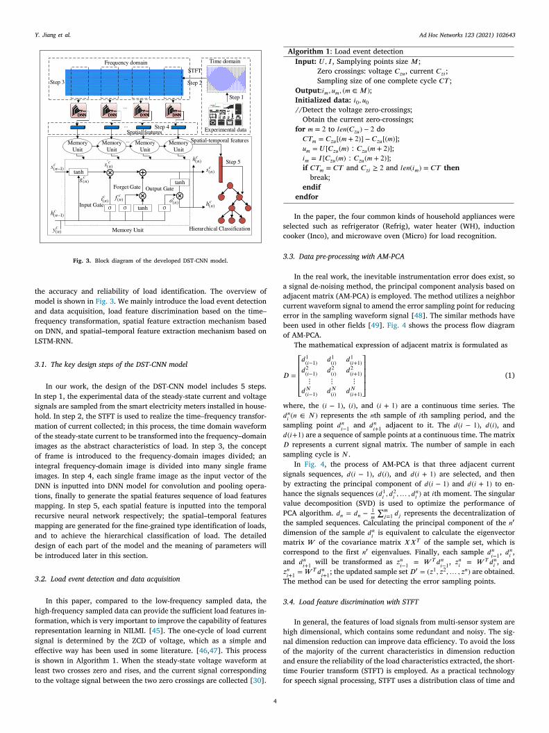
As the key component of DST-CNN model, DNN is employed torealize the spatial features extraction of the household appliances load.Fig. 7 demonstrates the schematic diagram of the load spatial featuresextracted. Briefly, the algorithm structure of DNN mainly includes twomainly parts: (1) features extractin from the frame image; (2) theconstruction of DNN structure for the spatial features extraction.

Step 1: feature extraction based on DNN. After the frequency-domain images of load have been obtained, the completefrequency-domain image of load is divided into some smaller frameimages, and then form a sequence of single frame images. In [51], theresult of the experiment confirms that a short-time property of framefeature is better than a long-time distributional frame pattern. Theprocess is as follows: we sample a frequency-domain image of load, thesequence 𝑋 with 𝑀 frames; by this way, the sequence frame is definedas 𝑅 =

∑𝑀𝑟=1 𝑅𝑖, where, 𝑅𝑖 is a frame, the value of 𝑖 is from 1 to 𝑀 . The

each frame 𝑅𝑖 as a feature vector is inputted to the first convolutionlayer of DNN, and then through the convolutional kernel layer to formthe features mapping. Each image of the sequence of frame images hasthe temporal characteristics, and each frame image of the sequenceframe images as a highly discriminative feature.

Step 2: construction of DNN structure for spatial features ex-traction. In this paper, to form the spatial feature representations ofload, a deep convolution neural network (DNN) is proposed. The struc-ture of DNN includes the convolution network layer, the max-pooling

5

layer, and the full-connection network layer. The number of parametersin each part is set to nine, six, and four respectively. Between theconvolution layer and maxi-pooling layer, we select rectified linearunit (ReLU) as the activation function. ReLU can boost the nonlinearityof function to avoid gradient descent. The expression of ReLU is asfollows:

ReLU(𝑥𝑖) = max(0, 𝑥𝑖) (3)

The feature map of the new convolution layers could be calculated as{

𝐶𝑛𝑖 = 𝜎(

∑

𝑠∈𝑀𝑖(𝑛−1)

∑

(𝑝,𝑞)∈𝐾(𝑛) 𝑤𝑠𝑖𝑠(𝑝,𝑞)𝑥

(𝑛−1)𝑠 (𝑐 + 𝑝, 𝑟 + 𝑞) + 𝑏(𝑛)𝑖 )

𝐾𝑛 = [(𝑝, 𝑞) ∈ 𝑁2|0 < 𝑝 < 𝑘𝑤, 0 < 𝑞 < 𝑘ℎ]

(4)

where, 𝐾 (𝑛) represents convolution kernel, 𝑛 indicates the number of theCNN layer, the size of convolution kernel is 𝐾𝑤 ×𝐾ℎ, the height is 𝐾ℎ,and the weight is 𝐾𝑤; 𝑏(𝑛)𝑖 is the bias of the 𝑖th characteristic mappingin convolution network layers, 𝑤𝑠

𝑖𝑠(𝑛−1) is the weight of the neuron ofthe 𝑖th feature mapping in convolution layers, 𝑠 is the previous state,the parameters 𝑐 and 𝑟 are the column and row of the input imagerespectively. The function 𝜎 represents the activation function ReLU.After the convolution layers, the features of image are inputted in themax-pooling, and to reduce overfitting. This detailed process can beformulated as:

𝑌 𝑛𝑖 = 𝑑𝑜𝑤𝑛(𝐶𝑛

𝑖 ) (5)

The 𝑑𝑜𝑤𝑛(∙) represents the down-sampling function, 𝐶𝑛𝑖 indicates

the features mapping. The max-pooling layer can reconstitute the newfeatures mapping with the max value of a filter 𝑛× 𝑛. In this process, ifthe inputed frame image is 𝑟𝑖(𝑥, 𝑦), after it through the first convolutionkernel 𝑘𝑖(𝑝, 𝑞) with the size 𝑎 × 𝑏, the corresponding feature mappingis 𝑚𝑖(𝑥, 𝑦), which can achieved the calculation by Eq. (4). After theconvolution layer, the feature mapping 𝑚𝑖(𝑥, 𝑦) will be inputted intothe max-pooling, and the size of the feature mapping transfers into𝑚′𝑖(𝑥, 𝑦) by Eq. (5), and then the features are extracted and fed into a

fully-connected layer. Finally, the spatial features mapping are formed,𝑠𝑚′

𝑖(𝑥, 𝑦), which is one-dimensional array, which will as the input layersare fed into the LSTM-RNN model.

3.6. Spatial–temporal feature extraction of DST-CNN model

In this section, we present a LSTM-RNN model to form the spatial–temporal feature mapping of the electricity load for the fine-grainedload identification. The structure of LSTM-RNN model is shown in

Ad Hoc Networks 123 (2021) 102643Y. Jiang et al.

Fig. 5. The time-domain steady-current waveform of 4 different appliances.(a1) Refrigerator. (b1) Water Heater. (c1) Micro-wave Oven.(d1) Induction Cooker.

Fig. 6. The frequency-domain images of 4 different appliances. (a2) Refrigerator. (b2) Water Heater. (c2) Micro-wave Oven. (d2) Induction Cooker.

Fig. 8. LSTM-RNN is used to solve the long dependency problem ofnetwork. In the paper, since the load has the characteristics of timeseries, LSTMs is used for the spatial–temporal feature extraction of theload. The detailed structure of the LSTMs is presented in Fig. 9.

The core of LSTMs model includes an input gate, a forget gate,and an output gate. The superscript 𝑐 of each vector represents theneuron, the subscript 𝑛 represents time, 𝑦(𝑛) represents the 𝑛 momentinput layer, and ℎ(𝑛−1) represents the (𝑛−1) moment hidden layer [52].The vector 𝑎𝑐(𝑛) is in the 𝑛 moment, the current state of LSTMs, and thecenter of each neuron has been linearly activated. Forget gate 𝑓 𝑐

(𝑛) isthe first step in the memory unit of LSTMs, which selectively deletecertain information of state. In the moment, 𝑓 𝑐

(𝑛) is used to controlledinformation of the input layer, and ℎ𝑐 is the previous moment of the

6

(𝑛−1)

hidden layer, and they determine the input of 𝑓 𝑐(𝑛). The expression of

𝑓 𝑐(𝑛) can be formulated as follows:

𝑓 𝑐(𝑛) = 𝜎(𝑊𝑓 ⋅ [ℎ𝑐(𝑛−1), 𝑦

𝑐(𝑛)] + 𝑏𝑓 ) (6)

The input gate and input node. The 𝑖𝑐(𝑛) represents the input gate ofthe LSTMs, and it is a sigmoid function layer to decide which value willbe updated. The 𝑔𝑐(𝑛) represent the input node, and it is a tanh functionlayer to create the candidate state vector 𝑎′𝑐(𝑛) states. The 𝑖𝑐(𝑛) is relatedto ℎ𝑐(𝑛−1) and 𝑦𝑐(𝑛). The calculation formula of 𝑖𝑐(𝑛) is defined as

𝑖𝑐 = 𝜎(𝑊 ⋅ [ℎ𝑐 , 𝑦𝑐 ] + 𝑏 ) (7)

(𝑛) 𝑖 (𝑛−1) (𝑛) 𝑖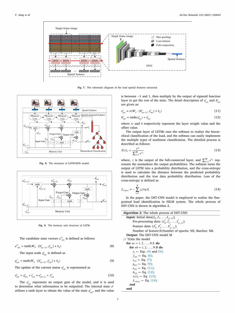

Ad Hoc Networks 123 (2021) 102643Y. Jiang et al.

Fig. 7. The schematic diagram of the load spatial features extracted.

Fig. 8. The structure of LSTM-RNN model.

Fig. 9. The memory unit structure of LSTM.

The candidate state vectors 𝑎′𝑐(𝑛) is defined as follows:

𝑎′𝑐(𝑛) = tanh(𝑊𝑎 ⋅ [ℎ𝑐(𝑛−1), 𝑦𝑐(𝑛)] + 𝑏𝑎) (8)

The input node 𝑔𝑐(𝑛) is defined as

𝑔𝑐(𝑛) = tanh(𝑊𝑔 ⋅ [ℎ𝑐(𝑛−1), 𝑦𝑐(𝑛)] + 𝑏𝑔) (9)

The update of the current status 𝑎𝑐(𝑛) is represented as

𝑎𝑐(𝑛) = 𝑔𝑐(𝑛) ∗ 𝑖𝑐(𝑛) + 𝑎𝑐(𝑛−1) ∗ 𝑓 𝑐(𝑛) (10)

The 𝑜𝑐(𝑛) represents an output gate of the model, and it is usedto determine what information to be outputted. The internal state 𝑎𝑐

utilizes a tanh layer to obtain the value of the state 𝑎𝑐 , and the value

7

(𝑛)

is between −1 and 1, then multiply by the output of sigmoid functionlayer to get the rest of the state. The detail description of 𝑜𝑐(𝑛) and ℎ𝑐(𝑛)are given as:

𝑜𝑐(𝑛) = 𝜎(𝑊𝑜 ⋅ [ℎ𝑐(𝑛−1), 𝑦𝑐(𝑛)] + 𝑏𝑜) (11)

ℎ𝑐(𝑛) = tanh(𝑎𝑐(𝑛)) ∗ 𝑜𝑐(𝑛) (12)

where 𝑤 and 𝑏 respectively represent the layer weight value and theoffset value.

The output layer of LSTMs uses the softmax to realize the hierar-chical classification of the load, and the softmax can easily implementthe multiple types of nonlinear classification. The detailed process isdescribed as follows:

𝑆(𝑧)𝑖 =𝑒𝑧𝑖

∑𝑀𝑗=1 𝑒

𝑧𝑗(13)

where, 𝑧 is the output of the full-connected layer, and ∑𝑀𝑗=1 𝑒

𝑧𝑗 rep-resents the normalizes the output probabilities. The softmax turns theoutput of LSTM into a probability distribution, and the cross-entropyis used to calculate the distance between the predicted probabilitydistribution and the true data probability distribution. Loss of thecross-entropy is defined as

𝐿𝑐𝑙𝑎𝑠𝑠 = −𝑁∑

𝑖=1𝑦𝑖𝑙𝑜𝑔𝑆𝑖 (14)

In the paper, the DST-CNN model is employed to realize the fine-grained load identification in NILM system. The whole process ofDST-CNN is shown in algorithm 2.

Algorithm 2: The whole process of DST-CNNInput: Initial data[𝐼0, 𝐼1,… , 𝐼(𝑡−1)];

Pre-processing data: [𝐼 ′

0, 𝐼′

1,… , 𝐼 ′

(𝑡−1)];Feature data: [𝐹 ′

0 , 𝐹′

1 ,… , 𝐹 ′

(𝑡−1)];Number of feature:N;Number of epochs: NE; Batches: NB.

Output: The DST-CNN model M// Train the model

for 𝑛𝑒 = 1, 2,… , 𝑁𝐸 dofor 𝑛𝑏 = 1, 2,… , 𝑁𝐵 do

𝑧𝑖 ← Eqs. (4) and (5);𝑓(𝑛) ← Eq. (6);𝑖(𝑛) ← Eq. (7);𝑔(𝑛) ← Eq. (9);𝑜(𝑛) ← Eq. (11);ℎ(𝑛) ← Eq. (12);𝑠(𝑧)𝑖 ← Eq. (13);𝐿𝑐𝑙𝑎𝑠𝑠 ← Eq. (14);

endend

Ad Hoc Networks 123 (2021) 102643Y. Jiang et al.

t

M

c

𝐿

v

wtbpa

𝑀

tlftRR

bta

3.7. Evaluation criterion of DST-CNN model

In our experiment, some practical evaluation criteria are employedfor the performance of the proposed model, namely the model accu-racy, Matthews correlation coefficient (MCC), Zero-loss score (ZL), andMacro − 𝐹1. The average value of all the precision is Macro − 𝐹1 score,he formula is describe as

acro − 𝐹1 =𝑖𝑀

𝑀∑

𝑚=1𝐹1(𝑚) (15)

where, the number of appliances is 𝑀 , 𝐹1(𝑚) is a weighted average ofmodel precision and recall rates of 𝑚th appliance, the maximum is 1,and the minimum is 0. The 𝐹1(𝑚) is defined as

𝐹1(𝑚) = 2 ⋅𝑝 ⋅ 𝑟𝑝 + 𝑟

(16)

where 𝑝 and 𝑟 represent the precision and the recall respectively.Zero-loss score (ZL) represents the 0_1 loss of classification, and the

alculating formula is deduced as

0−1(𝑥𝑘, 𝑥𝑘) = 1(𝑥𝑘 ≠ 𝑥𝑘) (17)

where assuming 𝑥𝑘 is the predictions of 𝑘th appliance, 𝑥𝑘 is the truealue of 𝑘th appliance.

MCC is called a balanced metric, and it can be used for classesith different sizes; MCC is a relational value between −1 and 1. If

he correlation coefficient is -1, and illustrates a complete inconsistencyetween prediction and observation; if the value is 1, and illustrates aerfect prediction, 0 shows an random prediction. MCC can be defineds follows:

𝐶𝐶 =𝑡𝑝𝑚 × 𝑡𝑛𝑚 − 𝑓𝑝𝑚 × 𝑓𝑛𝑚

√

(𝑡𝑝𝑚 + 𝑓𝑝𝑚)(𝑡𝑝𝑚 + 𝑓𝑛𝑚)(𝑡𝑛𝑚 + 𝑓𝑝𝑚)(𝑡𝑛𝑚 + 𝑓𝑛𝑚)(18)

In general, 𝑡𝑝𝑚, 𝑡𝑛𝑚, 𝑓𝑝𝑚, and 𝑓𝑛𝑚 represent the true positive, truenegative, false positive, and false negative of 𝑚th class respectively.

4. Experimental setups

This chapter presents that the real measured datasets are utilizedto train, test, and validate the proposed method. For better illustrationabout the performance advantage of the proposed method, three othertypical methods of load recognition are introduced. The simulationenvironment configuration includes Python 3.5, the PyTorch 1.0, andthe NVIDIA CUDA 9.0. Python 3.5 is used to program for the proposedalgorithm implementation.

4.1. Experiment datasets

In this paper, the experimental data acquisition are from 50 build-ings and the data collecting period is between 2018 and 2020. Thetime spent on using household appliances of one day is 24 h (samplingfrequency 𝑓𝑠 = 130). The data mainly includes four types of themost representative household appliances, namely refrigerator (Refrig),water heater (WH), microwave oven (Micro), and induction cooker(Inco). These data contain the steady-state voltage, current and activepower of the high-frequency load, which can provide the sufficientexperimental data sets for NILMI.

There are two key reasons to explain why we select the above fourkinds of electrical appliances to experiment. Firstly, the above selectedexperimental appliances are all the representative household appli-ances, and they are indispensable in modern life. Secondly, the changesin running state of those appliances are from simple to complex forms,and the variable running state samples are good for training modelsunder different conditions. Thirdly, considering the limited space of thepaper, the experiment only uses some common load combinations.

We use the relatively small data set No.1 building, No.2 buildingand No.3 building for experiment. There are 5 × 109 data samples

8

collected over the course of a year. These data samples consist of two

parts: the status data of the four kinds of electrical appliances workingalone; the status data of the simultaneous running of two or moreappliances. The sampling numbers of each type of appliances are 107

for training and testing model, which can provide the sufficient singleand multiple operating waveforms data.

To ensure the effectiveness of the acquired dataset, this experimenttakes the average of the three measurements as the final current value.Since existing the fluctuations of measuring signal, noise, and theabnormal spikes in sampling data, the AM-PCA is employed to completethe data pre-processing, which has been introduced in the previoussection. In the paper, the 80% datasets are selected to train the modeland the rest 20% to test the model.

4.2. The proposed model training and testing

For better illustration about the advantageous performance of theproposed method, the other three typical load recognition methods,namely KNN, CNN, and LSTM, are introduced to present the robustnessof our method in the paper. The parameters of DST-CNN model are setas the number of the hidden layer blocks is 5, each block consists of128 filters, and the filter size is 3. The pooling size and the poolingstride are all set to 2. ReLU is selected as the activation function, andthe value of the dropout probability is set to 0.5. The size of mini-batchis set to 512, the Adam optimizer is generally preferred and learningrate is set to 0.002. The number of epoch is set to 200 with an earlystopping criterion to prevent over-fitting.

In the experiment, we use the datasets from three buildings men-tioned above to discuss the experimental results of our proposedmethod. We performed 5-fold validation on each of the datasets. Theaccuracy of training process are reported in Fig. 10, where the bestresults are shown. From Fig. 10, among the training process of above4 models, the accuracy of DST-CNN method is the highest, and themean accuracy is 91.64%, which is 9.40% higher than the second-best ranked CNN. The CNN method has advantages for the imagerecognition, but for the recognition of load feature image based ontemporal characteristics, the accuracy is relatively low. The meanaccuracy of KNN and LSTM is 70.59% and 68.49%, respectively. TheLSTM is the lowest in four methods.

To further to analyze the performance of the proposed model, weused three testing dataset from three buildings to test the four model re-spectively, and we performed 3-fold validation on each of the datasets.By calculating the average value of the three verification results as thefinal results, the testing results are presented and discussed in Fig. 11.The results show that the testing accuracy of DST-CNN method is betterthan the other 3 models on the different testing datasets.

4.3. Evaluation criteria for the proposed model

To evaluate the performance of the proposed model, the single-label and the multi-label load identification are considered for ourexperiment. The Macro − 𝐹1 scores, ZL scores, and MCC are employedo evaluate the four types of load identification methods in the single-abel and the multi-label experiment. The experimental datasets arerom the three different buildings, each dataset includes the single andhe combined appliances, which are Refrig, WH, Micro, Inco, Re+WH,e+Micro, Re+Inco, Re+WH+Inco, Re+WH+Micro, Re+Micro+Inco,e+WH +Micro+Inco.

In Figs. 12 and 13, we use the three datasets from the differentuildings to verify the Macro−𝐹1 scores of the four method. It is obvioushat the DST-CNN method is better than the other three methods underll labeling conditions. In Fig. 12, it mainly demonstrates the Macro−𝐹1

scores of the single load identification test, and the Macro − 𝐹1 scoresof DST-CNN method are the best. The CNN method ranks the second,and better than the KNN and LSTM methods. In view of the time-seriescharacteristics of the load, the results clearly illustrate that the KNNand LSTM methods are inferior to DST-CNN and CNN methods. Fig. 13

Ad Hoc Networks 123 (2021) 102643Y. Jiang et al.

Fig. 10. The accuracy of training process.

Fig. 11. The accuracy of testing process.

Fig. 12. Macro − 𝐹1 scores of the single load identification test.

9

Fig. 13. Macro − 𝐹1 scores of the multi-load identification test.

presents the Macro−𝐹1 scores of the multi-load identification test, andthe Macro−𝐹1 scores of DST-CNN method is much better than the otherthree methods. In terms of the time series characteristic of load, theCNN method has no advantage in the multi-load recognizing. Theseresults obviously indicate that the DST-CNN method is effective for theload signal identification of NILMI under all labeling conditions.

The ZL scores and the MCC as the performance indicators are alsoused to evaluate the proposed model with the four methods and thetwo different datasets from two buildings (No.1 buildings and No.2buildings). In Tables 1, 2, and 3, the average scores and the standarddeviations of experimental are clearly demonstrated, and the boldscores represent the best results. Table 1 presents the results of fourmethods on the single load datasets, which are from the No. 1 buildingand No. 2 building respectively. The results show that the ZL scoresof DST-CNN method are less than the other three methods and theMCC scores are higher than the other three methods, indicating thatthe identification performance of DST-CNN method in the single loadis better. However, the MCC value of CNN method is the highest forrefrigerator identification, illuminating that CNN is an effective methodfor the single devices identification, and the case rarely occurs in thecombinatorial appliances identification.

The ZL scores and the MCC scores of the multi-labels experimentof the appliance identification can more deeply assess the proposed

Ad Hoc Networks 123 (2021) 102643Y. Jiang et al.

Table 1The key evaluation indexes of single appliances.

Index Method No. 1 building No. 2 building

Refrig WH Micro Inco Refrig WH Micro Inco

ZL

DST-CNN 10.47 𝟏.𝟏𝟖 𝟔.𝟓𝟒 𝟔.𝟐𝟑 9.11 𝟓.𝟑𝟐 𝟓.𝟑𝟎 𝟓.𝟗𝟕±0.13 ±𝟎.𝟎𝟐𝟏 ±𝟎.𝟏𝟔𝟏 ±𝟎.𝟏𝟕𝟑 ±0.112 ±𝟎.𝟏𝟐𝟒 ±𝟎.𝟎𝟗𝟏 ±𝟎.𝟎𝟏𝟑

KNN 27.01 24.45 18.99 19.01 21.13 25.14 19.13 19.18±0.062 ±0.038 ±0.012 ±0.043 ±0.052 ±0.089 ±0.045 ±0.012

CNN 𝟔.𝟑𝟎 15.54 13.47 14.50 𝟔.𝟐𝟕 9.46 10.43 11.49±𝟎.𝟎𝟑𝟔 ±0.012 ±0.031 ±0.057 ±𝟎.𝟎𝟏𝟒 ±0.011 ±0.023 ±0.009

LSTM 27.88 26.73 28.05 26.52 27.49 28.17 26.41 25.72±0.045 ±0.034 ±0.052 ±0.018 ±0.023 ±0.019 ±0.015 ±0.016

MCC

DST-CNN 0.88 𝟎.𝟗𝟗 𝟎.𝟗𝟐 𝟎.𝟗𝟑 0.90 𝟎.𝟗𝟓 𝟎.𝟗𝟓 𝟎.𝟗𝟒±0.035 ±𝟎.𝟎𝟏𝟒 ±𝟎.𝟎𝟐𝟐 ±𝟎.𝟎𝟏𝟏 ±0.014 ±𝟎.𝟎𝟏𝟒 ±𝟎.𝟎𝟐𝟏 ±𝟎.𝟎𝟎𝟗

KNN 0.70 0.74 0.79 0.78 0.77 0.73 0.78 0.78±0.025 ±0.021 ±0.031 ±0.014 ±0.017 ±0.016 ±0.025 ±0.021

CNN 𝟎.𝟗𝟑 0.82 0.85 0.84 𝟎.𝟗𝟑 0.89 0.88 0.87±𝟎.𝟎𝟏𝟎 ±0.009 ±0.021 ±0.045 ±𝟎.𝟎𝟑𝟖 ±0.051 ±0.047 ±0.031

LSTM 0.69 0.70 0.68 0.70 0.69 0.66 0.71 0.72±0.023 ±0.031 ±0.015 ±0.014 ±0.053 ±0.063 ±0.062 ±0.013

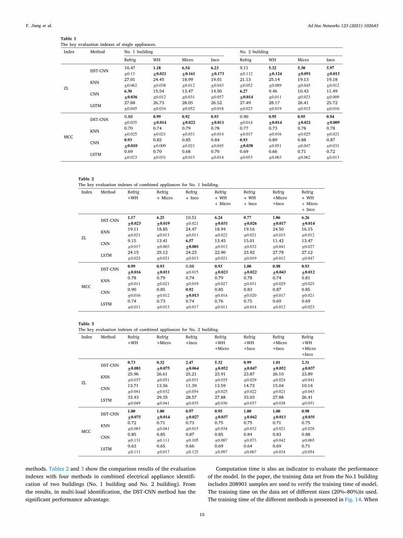
Table 2The key evaluation indexes of combined appliances for No. 1 building.

Index Method Refrig+WH

Refrig+ Micro

Refrig+ Inco

Refrig+ WH+ Micro

Refrig+ WH+ Inco

Refrig+Micro+Inco

Refrig+ WH+ Micro+ Inco

ZL

DST-CNN 𝟏.𝟏𝟕 𝟔.𝟐𝟓 10.51 𝟔.𝟐𝟒 𝟎.𝟕𝟕 𝟏.𝟖𝟔 𝟔.𝟐𝟔±𝟎.𝟎𝟐𝟑 ±𝟎.𝟎𝟏𝟗 ±0.021 ±𝟎.𝟎𝟑𝟏 ±𝟎.𝟎𝟐𝟔 ±𝟎.𝟎𝟏𝟕 ±𝟎.𝟎𝟏𝟒

KNN 19.11 18.85 24.47 18.94 19.16 24.50 16.15±0.021 ±0.013 ±0.011 ±0.022 ±0.021 ±0.015 ±0.012

CNN 9.15 13.41 𝟔.𝟓𝟕 13.45 15.01 11.42 13.47±0.017 ±0.003 ±𝟎.𝟎𝟎𝟏 ±0.012 ±0.032 ±0.041 ±0.027

LSTM 24.15 25.12 24.23 22.90 23.92 27.78 27.12±0.025 ±0.021 ±0.013 ±0.021 ±0.019 ±0.012 ±0.047

MCC

DST-CNN 𝟎.𝟗𝟗 𝟎.𝟗𝟑 0.88 𝟎.𝟗𝟑 𝟏.𝟎𝟎 𝟎.𝟗𝟖 𝟎.𝟗𝟑±𝟎.𝟎𝟏𝟔 ±𝟎.𝟎𝟏𝟏 ±0.015 ±𝟎.𝟎𝟐𝟑 ±𝟎.𝟎𝟐𝟐 ±𝟎.𝟎𝟒𝟑 ±𝟎.𝟎𝟏𝟐

KNN 0.78 0.79 0.74 0.79 0.78 0.74 0.81±0.011 ±0.021 ±0.019 ±0.027 ±0.031 ±0.029 ±0.025

CNN 0.90 0.85 𝟎.𝟗𝟐 0.85 0.83 0.87 0.85±0.016 ±0.012 ±𝟎.𝟎𝟏𝟑 ±0.014 ±0.020 ±0.017 ±0.021

LSTM 0.74 0.73 0.74 0.76 0.75 0.69 0.69±0.011 ±0.013 ±0.017 ±0.011 ±0.014 ±0.012 ±0.023

Table 3The key evaluation indexes of combined appliances for No. 2 building.

Index Method Refrig+WH

Refrig+Micro

Refrig+Inco

Refrig+WH+Micro

Refrig+WH+Inco

Refrig+Micro+Inco

Refrig+WH+Micro+Inco

ZL

DST-CNN 𝟎.𝟕𝟑 𝟎.𝟑𝟐 𝟐.𝟒𝟕 𝟓.𝟑𝟐 𝟎.𝟗𝟗 𝟏.𝟎𝟏 𝟐.𝟑𝟏±𝟎.𝟎𝟖𝟏 ±𝟎.𝟎𝟕𝟓 ±𝟎.𝟎𝟔𝟒 ±𝟎.𝟎𝟓𝟐 ±𝟎.𝟎𝟒𝟕 ±𝟎.𝟎𝟓𝟐 ±𝟎.𝟎𝟑𝟕

KNN 25.96 26.61 25.21 23.91 23.87 26.10 23.89±0.037 ±0.051 ±0.031 ±0.035 ±0.029 ±0.024 ±0.041

CNN 13.71 13.56 11.39 13.59 14.72 15.04 10.14±0.041 ±0.032 ±0.054 ±0.025 ±0.022 ±0.021 ±0.043

LSTM 33.43 29.35 28.57 27.88 33.03 27.88 26.41±0.049 ±0.041 ±0.035 ±0.036 ±0.037 ±0.038 ±0.031

MCC

DST-CNN 𝟏.𝟎𝟎 𝟏.𝟎𝟎 𝟎.𝟗𝟕 𝟎.𝟗𝟓 𝟏.𝟎𝟎 𝟏.𝟎𝟎 𝟎.𝟗𝟖±𝟎.𝟎𝟕𝟓 ±𝟎.𝟎𝟏𝟒 ±𝟎.𝟎𝟐𝟕 ±𝟎.𝟎𝟑𝟕 ±𝟎.𝟎𝟒𝟐 ±𝟎.𝟎𝟏𝟑 ±𝟎.𝟎𝟑𝟓

KNN 0.72 0.71 0.73 0.75 0.75 0.71 0.75±0.083 ±0.041 ±0.015 ±0.034 ±0.032 ±0.021 ±0.028

CNN 0.85 0.85 0.87 0.85 0.84 0.83 0.88±0.131 ±0.111 ±0.105 ±0.087 ±0.073 ±0.042 ±0.065

LSTM 0.63 0.65 0.66 0.69 0.64 0.69 0.71±0.111 ±0.017 ±0.125 ±0.097 ±0.067 ±0.034 ±0.054

methods. Tables 2 and 3 show the comparison results of the evaluationindexes with four methods in combined electrical appliance identifi-cation of two buildings (No. 1 building and No. 2 building). Fromthe results, in multi-load identification, the DST-CNN method has thesignificant performance advantage.

10

Computation time is also an indicator to evaluate the performanceof the model. In the paper, the training data set from the No.1 buildingincludes 208901 samples are used to verify the training time of model.The training time on the data set of different sizes (20%–80%)is used.The training time of the different methods is presented in Fig. 14. When

Ad Hoc Networks 123 (2021) 102643Y. Jiang et al.

Fig. 14. Comparison of training time on the different size of data set.

the size of the data set is only 20%, the training time of CNN model isthe shortest. As the size of the data set increasing, the DST-CNN modelis the fastest than the other models. However, the training time is alsodepends on the size of the training dataset and the performance of thecomputer. The performance of DST-CNN model and the outstandingcharacterization learning ability can improve the computation time.

4.4. Residential households load identification experiment

In this section, the performance and practicability of our methodin residential households load identification are verified. We randomlysampled the real steady-state current signals in No. 3 building in anythree days of May, and the sampling period is 24 h of one day inFig. 15(a). From the figure, the main power consumption time ofhousehold equipment contains 6:00 a.m.-8:00 a.m., 11:00 a.m.-1:00p.m., 6:00 p.m.-8:00 p.m., and 9:00 p.m.-10:30 p.m.. Considering theimaginable error in raw data set, the method of event detection andpre-processing are used, and used the DST-CNN method to realize theload identification. The frequency-domain characteristic map and theexperimental results are showed in Fig. 15(b), Fig. 16, respectively.

From Fig. 16, the results of load identification for the four typesof household appliance loads are clearly showed, and the each rowrepresents a complete collection date cycle, which according to thethree datasets in Fig. 15. Induction cooker and water heater work in thesame pattern, refrigerator and micro-wave oven work in three differenttypes work patterns respectively, and each work pattern present adifferent current characteristic waveform.

In the residential households loads identification experiment, a com-plete experimental process is clearly presented, and these results prove

11

Fig. 16. The results of residential load identification in No. 3 family.

the practicability of the proposed method for NILMI. These results alsodemonstrate that our model can improve the ability of load abstractfeature representation and the accuracy of the load fine-grained iden-tification. Especially, in the multi-load identification experiment, thecomplex load features are accurately captured, which concludes thatthe complex state of load can be considered as a combination of thesingle state. Using the representative dataset to validate the proposedmethod, and it demonstrates that the method can improve the accuracyof load feature extraction and identification. Using the different datasets to validate the method, and it demonstrates the high reliability.

5. Conclusions

In this article, a reliable deep learning-based algorithm frameworkfor IoT loads identification, DST-CNN, is proposed to address the prob-lems of the incomplete discrimination of load feature, the accuracyand reliability of the identification mode, and the generalization andglobal optimization. DST-CNN method enhances the effectiveness of theload signal by AM-PCA method, improves the ability of load abstractcharacteristics representation by reconstructing DNN, and achieves thefine-grained accurate identification of load by a LSTM-RNN with thespatio-temporal feature recognition mechanism. The significant perfor-mance improvements of our proposed method are verified by extensiveexperiments. Applying the proposed method help to establish the hier-archical knowledge base of electrical equipment, which covering theinformation such as power, operating mode and time consumption.This way can help the demand-side of the smart grids to accuratelyobtain the power consumption information of the user, and increase the

Fig. 15. The time-domain waveform and the frequency feature map.(a)The time-domain waveform.(b)The frequency feature mapping.

Ad Hoc Networks 123 (2021) 102643Y. Jiang et al.

electric power efficiency of the customers and load shifting in IoT loadmonitoring system. In our future work, DST-CNN will be used on themore complex data sets, without reducing the accuracy of recognitionand adding the time complexity.

Declaration of competing interest

The authors declare that they have no known competing finan-cial interests or personal relationships that could have appeared toinfluence the work reported in this paper.

Acknowledgment

The authors of this paper were supported by S&T Program of Hebeithrough grant 20310101D.

References

[1] T. Wang, M.Z.A. Bhuiyan, G. Wang, M.A. Rahman, J. Wu, J. Cao, Big datareduction for a smart city’s critical infrastructural health monitoring, IEEECommun. Mag. 56 (3) (2018) 128–133.

[2] D. Garcia-Perez, D. Perez-Lopez, I. Diaz-Blanco, A. Gonzalez-Muniz, A.A.Cuadrado-Vega, Fully-convolutional denoising auto-encoders for NILM in largenon-residential buildings, IEEE Trans. Smart Grid PP (99) (2020) 1.

[3] R. Jones, A. Rodriguez-Silva, S. Makonin, Increasing the accuracy and speed ofuniversal non-intrusive load monitoring (UNILM) using a novel real- time steady-state block filter, in: Proceedings of the IEEE Power & Energy Society InnovativeSmart Grid Technologies Conference, ISGT, 2020.

[4] H. Imen, N. Etinkaya, J.C. Vasquez, J.M. Guerrero, A microgrid energy man-agement system based on non-intrusive load monitoring via multitask learning,IEEE Trans. Smart Grid 12 (2) (2020).

[5] S. Wang, L. Du, J. Ye, D. Zhao, Deep generative model for non-intrusiveidentification of EV charging profiles, IEEE Trans. Smart Grid PP (99) (2020)1.

[6] A. Faustine, L. Pereira, C. Klemenjak, Adaptive weighted recurrence graphs forappliance recognition in non-intrusive load monitoring, IEEE Trans. Smart GridPP (99) (2020) 1.

[7] H. Tao, M.Z.A. Bhuiyan, M.A. Rahman, T. Wang, J. Wu, a. Salih, T. Hayajneh,Trustdata: Trustworthy and secured data collection for event detection inindustrial cyber-physical system, IEEE Trans. Ind. Inf. 16 (5) (2020) 3311–3321.

[8] L. Pereira, N. Nunes, An empirical exploration of performance metrics for eventdetection algorithms in non-intrusive load monitoring, Sustainable Cities Soc.(2020) 102399.

[9] G. Rajendiran, M. Kumar, C. Joshua, K. Srinivas, Energy management usingnon-intrusive load monitoring techniques - state-of-the-art and future researchdirections, Sustainable Cities Soc. 62 (2020) 102411.

[10] W. Kong, Z.Y. Dong, B. Wang, J. Zhao, J. Huang, A practical solution for non-intrusive type II load monitoring based on deep learning and post-processing,IEEE Trans. Smart Grid PP (99) (2019) 1.

[11] M.A. Mengistu, A.A. Girmay, C. Camarda, A. Acquaviva, E. Patti, A cloud-basedon-line disaggregation algorithm for home appliance loads, IEEE Trans. SmartGrid (2018) 1.

[12] J. Wang, G. Geng, K.L. Chen, H. Liang, W. Xu, Event-based non-intrusive homecurrent measurement using sensor array, IEEE Trans. Smart Grid (2017) 1.

[13] N. Henao, K. Agbossou, S. Kelouwani, Y. Dube, M. Fournier, Approach innonintrusive type I load monitoring using subtractive clustering, IEEE Trans.Smart Grid PP (2) (2015) 1.

[14] S. Singh, A. Majumdar, Non-intrusive load monitoring via multi-label sparserepresentation-based classification, IEEE Trans. Smart Grid PP (99) (2019) 1.

[15] S. Pascal A., M. Iosif, Statistical and electrical features evaluation for electricalappliances energy disaggregation, Sustainability 11 (3222) (2019).

[16] Bonfigli, Roberto, Felicetti, Andrea, Principi, Emanuele, Fagiani, Marco, Squar-tini, Stefano, Denoising autoencoders for non-intrusive load monitoring:Improvements and comparative evaluation, Energy Build. (2018).

[17] X. Wu, D. Jiao, Y. Du, Automatic implementation of a self-adaption non-intrusiveload monitoring method based on the convolutional neural network, Processes(2020).

[18] D. Zhao, C. Chen, Z. Fang, Non-intrusive appliance identification withappliance-specific networks, IEEE Trans. Ind. Appl. (2020).

[19] R. Gopinath, M. Kumar, K. Srinivas, Feature mapping based deep neuralnetworks for non-intrusive load monitoring of similar appliances in buildings,in: Proceedings of the in The 7th ACM International Conference on Systems forEnergy-Efficient Buildings, Cities, and Transportation, BuildSys ’20, 2020.

[20] S. Mohamad, H. Bouchachia, Deep online hierarchical dynamic unsupervisedlearning for pattern mining from utility usage data, Neurocomputing (2019).

[21] Q. Zhao, Y. Xu, Z. Wei, Y. Han, Non-intrusive load monitoring based on deeppairwise-supervised hashing to detect unidentified appliances, Processes 9 (3)

12

(2021) 505.

[22] F. Ciancetta, G. Bucci, E. Fiorucci, S. Mari, A. Fioravanti, A new convolutionalneural network-based system for NILM applications, IEEE Trans. Instrum. Meas.PP (99) (2020) 1.

[23] Y. Tian, H. Wang, A. Li, S. Shi, J. Wu, Non-intrusive load monitoring usinginception structure deep learning, in: 2020 10th International Conference onPower and Energy Systems, ICPES, 2020.

[24] K. Jihyun, T. Le, K. Howon, Nonintrusive load monitoring based on advanceddeep learning and novel signature, Comput. Intell. Neurosci. 2017 (2017)4216281.

[25] K. He, L. Stankovic, L. Jing, V. Stankovic, Non-intrusive load disaggregationusing graph signal processing, IEEE Trans. Smart Grid 9 (3) (2018) 1739–1747.

[26] S. Singh, A. Majumdar, Non-intrusive load monitoring via multi-label sparserepresentation-based classification, IEEE Trans. Smart Grid PP (99) (2019) 1.

[27] M. Qureshi, C. Ghiaus, N. Ahmad, A blind event-based learning algorithm fornon-intrusive load disaggregation, Int. J. Electr. Power Energy Syst. 129 (1)(2021) 106834.

[28] Q. Liu, K.M. Kamoto, X. Liu, M. Sun, N. Linge, Low-complexity non-intrusiveload monitoring using unsupervised learning and generalized appliance models,IEEE Trans. Consum. Electron. 65 (1) (2019) 28–37.

[29] N. Chumrit, C. Weangwan, N. Aunsri, ECG-based Arrhythmia detection usingaverage energy and zero-crossing features with support vector machine, in:2020-5th International Conference on Information Technology, InCIT, 2021.

[30] D.S. Yang, X.T. Gao, L. Kong, Pang, An event-driven convolutional neuralarchitecture for non-intrusive load monitoring of residential appliance, IEEETrans. Consum. Electron. 66 (2) (2020) 137–182.

[31] JiangJie, KongQiuqiang, D. Plumbleymark, GilbertNigel, HoogendoornMark, M.Roijersdiederik, Deep learning-based energy disaggregation and on/off detectionof household appliances, ACM Trans. Knowl. Discov. Data (2021).

[32] S. Houidi, D. Fourer, F. Auger, On the use of concentrated time-frequencyrepresentations as input to a deep convolutional neural network: Applicationto non intrusive load monitoring, Entropy 22 (9) (2020).

[33] J. Zhang, X. Chen, W. Ng, C.S. Lai, L.L. Lai, New appliance detection fornon-intrusive load monitoring, IEEE Trans. Ind. Inf. PP (99) (2019) 1.

[34] A. Wang, Longjun, B. Chen, C. Xiaomin, Gang, D. Hua, Non-intrusive loadmonitoring algorithm based on features of V-I trajectory, Electr. Power Syst.Res. 157 (Apr.) (2018) 134–144.

[35] N. Miao, S. Zhao, Q. Shi, R. Zhang, Non-intrusive load disaggregation using semi-supervised learning method, in: Proceedings of the 2019 International Conferenceon Security, Pattern Analysis, and Cybernetics, SPAC, 2020.

[36] Y.H. Lin, A parallel evolutionary computing-embodied artificial neural networkapplied to non-intrusive load monitoring for demand-side management in a smarthome: Towards deep learning, Sensors 20 (6) (2020) 1649.

[37] G. Cui, B. Liu, W. Luan, et al., Estimation of target appliance electricityconsumption using background filtering, IEEE Trans. Smart Grid 1 (2019).

[38] B. Hs, A. Sm, B. Mt, Unsupervised Bayesian non parametric approach for non-intrusive load monitoring based on time of usage - sciencedirect, Neurocomputing(2021).

[39] D. Su, Q. Shi, H. Xu, W. Wang, Nonintrusive load monitoring based oncomplementary features of spurious emissions, ELECTRONICS (2019).

[40] M. Xia, W. Liu, K. Wang, W. Song, C. Chen, Y. Li, Non-intrusive load disag-gregation based on composite deep long short-term memory network, J. Magn.Mater. Dev. 160 (113669) (2020).

[41] M.C. Pegalajar, L. Ruiz, M. Cuéllar, R. Rueda, Analysis and enhanced predictionof the Spanish electricity network through big data and machine learningtechniques, Internat. J. Approx. Reason. 133 (11) (2021).

[42] G. M. Junaid, U. Gul Malik, P. Anand, M. Jihoon, R. Seungmin, Mid-termelectricity load prediction using CNN and Bi-LSTM, J. Supercomput. (2021).

[43] H. Zhou, D. Ren, H. Xia, M. Fan, H. Huang, AST-GNN: AN attention-basedspatio-temporal graph neural network for interaction-aware pedestrian trajectoryprediction, Neurocomputing (2021).

[44] X. Yin, G. Wu, J. Wei, Y. Shen, B. Yin, Multi-stage attention spatial-temporalgraph networks for traffic prediction, Neurocomputing 428 (6) (2020).

[45] E. Luo, M.Z.A. Bhuiyan, G. Wang, M.A. Rahman, J. Wu, M. Atiquzzaman, Pri-vacyprotector: Privacy-protected patient data collection in IoT-based healthcaresystems, IEEE Commun. Mag. 56 (2) (2018) 163–168.

[46] A. Faustine, L. Pereira, Improved appliance classification in non-intrusive loadmonitoring using weighted recurrence graph and convolutional neural networks,Energies 13 (2020).

[47] Zain, J. Mohamad, Hayajneh, Thaier, Abdalla, N. Ahmed, Hassan, M. Mehedi,Bhuiyan, M.Z.a. Alam, Secured data collection with hardware-based ciphers forIoT-based healthcare, IEEE Internet Things J. (2019).

[48] J.A. Cadzow, Signal enhancement-a composite property mapping algorithm,Acoust Speech Signal Process IEEE Trans 36 (1) (1988) 49–62.

[49] X. Peng, M. Bergsneider, H. Xiao, Pulse onset detection using neighborpulse-based signal enhancement, Med. Eng. Phy. 31 (3) (2009) 337–345.

[50] M. Lin, M. Tsai, Development of an improved time–frequency analysis-basednonintrusive load monitor for load demand identification, IEEE Trans. Instrum.Meas. 63 (6) (2014) 1470–1483.

[51] K. Jihyun, L. Thi-Thu-Huong, K. Howon, Nonintrusive load monitoring basedon advanced deep learning and novel signature, Comput. Intell. Neurosci. 2017(2017) 4216281.

[52] H. Peng, J. Li, Q. Gong, Y. Ning, L. He, Motif-matching based subgraph-levelattentional convolutional network for graph classification, in: Proceedings of theAAAI Conference on Artificial Intelligence, Vol. 34, No. 4, 2020, pp. 5387–5394.

Ad Hoc Networks 123 (2021) 102643Y. Jiang et al.

Yanmei Jiang is currently working toward the Ph.D. degreeat State Key Laboratory of Reliability and Intelligence ofElectrical Equipment in Hebei University of Technology. Hisresearch interests include machine learning, application ofintelligent power equipment,Internet of Things reliability.

Mingsheng Liu is currently a professorat State Key Labora-tory of Reliability and Intelligence of Electrical Equipmentin Hebei University of Technology. His research focuseson network and information security, computer networktechnology and application, big data.

13

Hao Peng is currently an Assistant Professor at the School ofCyber Science and Technology, and Beijing Advanced Inno-vation Center for Big Data and Brain Computing in BeihangUniversity. His research interests include representationlearning, machine learning and graph mining.

Md Zakirul Alam Bhuiyan(Senior Member, IEEE) wasas an Assistant Professor with Temple University and aPostdoctoral Research Fellow with the School of InformationScience and Engineering, Central South University. He iscurrently an Assistant Professor with the Department ofComputer and Information Sciences, Fordham University,NY, USA. His research focuses on dependability, cyberse-curity, big data, and cyber physical systems. He is also amember of ACM.