A RELIABILITY ASSESSMENT METHODOLOGY FOR …

A RELIABILITY ASSESSMENT METHODOLOGY FOR

DISTRIBUTION SYSTEMS WITH DISTRIBUTED GENERATION

A Thesis

by

SUCHISMITA SUJAYA DUTTAGUPTA

Submitted to the Office of Graduate Studies ofTexas A&M University

in partial fulfillment of the requirements for the degree of

MASTER OF SCIENCE

May 2006

Major Subject: Electrical Engineering

brought to you by COREView metadata, citation and similar papers at core.ac.uk

provided by Texas A&M University

https://core.ac.uk/display/147125479?utm_source=pdf&utm_medium=banner&utm_campaign=pdf-decoration-v1

A RELIABILITY ASSESSMENT METHODOLOGY FOR

DISTRIBUTION SYSTEMS WITH DISTRIBUTED GENERATION

A Thesis

by

SUCHISMITA SUJAYA DUTTAGUPTA

Submitted to the Office of Graduate Studies ofTexas A&M University

in partial fulfillment of the requirements for the degree of

MASTER OF SCIENCE

Approved by:

Chair of Committee, Chanan SinghCommittee Members, Mehrdad Ehsani

Shankar P. BhattacharyyaAlexander G. Parlos

Head of Department, Costas N. Georghiades

May 2006

Major Subject: Electrical Engineering

iii

ABSTRACT

A Reliability Assessment Methodology for

Distribution Systems with Distributed Generation. (May 2006)

Suchismita Sujaya Duttagupta, B.S., Louisiana State University

Chair of Advisory Committee: Dr. Chanan Singh

Reliability assessment is of primary importance in designing and planning dis-

tribution systems that operate in an economic manner with minimal interruption of

customer loads. With the advances in renewable energy sources, Distributed Genera-

tion (DG), is forecasted to increase in distribution networks. The study of reliability

evaluation of such networks is a relatively new area. This research presents a new

methodology that can be used to analyze the reliability of such distribution systems

and can be applied in preliminary planning studies for such systems. The method uses

a sequential Monte Carlo simulation of the distribution system’s stochastic model to

generate the operating behavior and combines that with a path augmenting Max flow

algorithm to evaluate the load status for each state change of operation in the system.

Overall system and load point reliability indices such as hourly loss of load, frequency

of loss of load and expected energy unserved can be computed using this technique.

On addition of DG in standby mode of operation at specific locations in the net-

work, the reliability indices can be compared for different scenarios and strategies for

placement of DG and their capacities can be determined using this methodology.

iv

ACKNOWLEDGMENTS

I would like to express sincere gratitude to my advisor, Dr. Chanan Singh, for

his invaluable support and guidance. He gave important insights into the research

problem and I appreciate his patience and encouragement throughout the course of

my graduate studies. I thankfully acknowledge my committee members, Dr. Ehsani,

Dr. Bhattacharyya and Dr. Parlos for their time and suggestions.

I would like to thank my parents and brother for their unwavering concern and

encouragement that was always a source of motivation for me. Words are insufficient

to express gratitude to my husband for his selfless love and support.

This research was supported by the National Science Foundation Grant ECS

0406794: Exploring the Future of Distributed Generation and Micro-Grid Networks.

v

TABLE OF CONTENTS

CHAPTER Page

I INTRODUCTION . . . . . . . . . . . . . . . . . . . . . . . . . . 1

A. Introduction . . . . . . . . . . . . . . . . . . . . . . . . . . 1

B. Distribution System Reliability . . . . . . . . . . . . . . . 2

C. Distributed Generation . . . . . . . . . . . . . . . . . . . . 2

D. Literature Review . . . . . . . . . . . . . . . . . . . . . . . 3

E. Outline of Thesis . . . . . . . . . . . . . . . . . . . . . . . 8

II RELIABILITY EVALUATION OF A DISTRIBUTION NET-

WORK . . . . . . . . . . . . . . . . . . . . . . . . . . . . . . . . 10

A. Overview of a distribution network . . . . . . . . . . . . . 10

B. Adequacy vs. Security . . . . . . . . . . . . . . . . . . . . 10

C. Comparison of Indices . . . . . . . . . . . . . . . . . . . . 11

D. Probabilistic Indices . . . . . . . . . . . . . . . . . . . . . 12

1. Hourly Loss of Load Expectation . . . . . . . . . . . . 12

2. Loss of Load Frequency . . . . . . . . . . . . . . . . . 12

3. Expected Unserved Energy . . . . . . . . . . . . . . . 12

III SIMULATION METHODOLOGY . . . . . . . . . . . . . . . . . 13

A. Monte Carlo Simulation Theory . . . . . . . . . . . . . . . 13

1. Sequential and Sampling Simulations . . . . . . . . . . 13

a. Next Event Method . . . . . . . . . . . . . . . . 14

B. Flow Criterion in Power Network . . . . . . . . . . . . . . 14

C. Theory on the Ford-Fulkerson Algorithm . . . . . . . . . . 21

D. Implementation . . . . . . . . . . . . . . . . . . . . . . . . 24

1. Architecture . . . . . . . . . . . . . . . . . . . . . . . 24

a. Discrete Event Simulator . . . . . . . . . . . . . 25

b. Monte Carlo . . . . . . . . . . . . . . . . . . . . 26

c. Max-Flow . . . . . . . . . . . . . . . . . . . . . 26

d. Collection of Statistics . . . . . . . . . . . . . . 27

e. Visualization . . . . . . . . . . . . . . . . . . . . 28

2. Simulation Procedure . . . . . . . . . . . . . . . . . 29

3. Performance Enhancements . . . . . . . . . . . . . . 30

a. Early Prototype . . . . . . . . . . . . . . . . . . 30

vi

CHAPTER Page

b. Time-Varying Loads . . . . . . . . . . . . . . . 30

c. Max-Flow Cache/Precomputation . . . . . . . . 31

IV SYSTEM MODEL . . . . . . . . . . . . . . . . . . . . . . . . . 32

A. Component Model . . . . . . . . . . . . . . . . . . . . . . 32

B. Small System Illustration . . . . . . . . . . . . . . . . . . . 32

1. Analytical Approach . . . . . . . . . . . . . . . . . . . 33

2. Developed Simulation Methodology . . . . . . . . . . 39

C. Distribution System Data . . . . . . . . . . . . . . . . . . 40

1. Distributions for Component Models . . . . . . . . . . 41

2. Load Models . . . . . . . . . . . . . . . . . . . . . . . 43

V CASE STUDIES . . . . . . . . . . . . . . . . . . . . . . . . . . 47

A. BUS 2 Reliability Results . . . . . . . . . . . . . . . . . . 47

1. Supply Capacity of 20 MW . . . . . . . . . . . . . . . 48



B. BUS 4 Reliability Results . . . . . . . . . . . . . . . . . . 60




VI CONCLUSIONS . . . . . . . . . . . . . . . . . . . . . . . . . . . 77

REFERENCES . . . . . . . . . . . . . . . . . . . . . . . . . . . . . . . . . . . 78

APPENDIX A . . . . . . . . . . . . . . . . . . . . . . . . . . . . . . . . . . . 81

VITA . . . . . . . . . . . . . . . . . . . . . . . . . . . . . . . . . . . . . . . . 90

vii

LIST OF TABLES

TABLE Page

I Load Model . . . . . . . . . . . . . . . . . . . . . . . . . . . . . . . 33

II Generation System Model Indices . . . . . . . . . . . . . . . . . . . 37

III Load Model Indices . . . . . . . . . . . . . . . . . . . . . . . . . . . 37

IV Margin Availability between Load Demand and Generation Ca-

pacity Levels . . . . . . . . . . . . . . . . . . . . . . . . . . . . . . . 38

V Comparison of System Level Indices for Bus 2 Supply of 20 MW . . 50

VI Comparison of System Level Indices for Bus 2 Supply of 30 MW . . 55

VII Comparison of System Level Indices for Bus 2 Supply of 40 MW . . 59

VIII Comparison of System Level Indices for Bus 4 Supply of 40 MW . . 64

IX Comparison of System Level Indices for Bus 4 Supply of 60 MW . . 70

X Comparison of System Level Indices for Bus 4 Supply of 80 MW . . 75

XI Bus 2 Results, Supply Capacity 20 MW . . . . . . . . . . . . . . . . 81

XII Bus 2 Results, Supply Capacity 30 MW . . . . . . . . . . . . . . . . 82

XIII Bus 2 Results, Supply Capacity 40 MW . . . . . . . . . . . . . . . . 83

XIV Bus 4 Results, Supply Capacity 40 MW . . . . . . . . . . . . . . . . 84

XV Bus 4 Results, Supply Capacity 60 MW . . . . . . . . . . . . . . . . 86

XVI Bus 4 Results, Supply Capacity 80 MW . . . . . . . . . . . . . . . . 87

viii

LIST OF FIGURES

FIGURE Page

1 Sample Distribution Network . . . . . . . . . . . . . . . . . . . . . . 11

2 Flow Graph . . . . . . . . . . . . . . . . . . . . . . . . . . . . . . . 15

3 Flow 1 . . . . . . . . . . . . . . . . . . . . . . . . . . . . . . . . . . 16

4 Flow 2 . . . . . . . . . . . . . . . . . . . . . . . . . . . . . . . . . . 17

5 Flow 3 . . . . . . . . . . . . . . . . . . . . . . . . . . . . . . . . . . 17

6 Flow 4 . . . . . . . . . . . . . . . . . . . . . . . . . . . . . . . . . . 18

7 Flow 5 . . . . . . . . . . . . . . . . . . . . . . . . . . . . . . . . . . 18

8 Flow 6 . . . . . . . . . . . . . . . . . . . . . . . . . . . . . . . . . . 19

9 Flow 7 . . . . . . . . . . . . . . . . . . . . . . . . . . . . . . . . . . 19

10 Flow 8 . . . . . . . . . . . . . . . . . . . . . . . . . . . . . . . . . . 20

11 Flow 9 . . . . . . . . . . . . . . . . . . . . . . . . . . . . . . . . . . 21

12 Flow 10 . . . . . . . . . . . . . . . . . . . . . . . . . . . . . . . . . . 22

13 Flow chart for the Ford-Fulkerson Algorithm . . . . . . . . . . . . . 23

14 2-State Markov Model . . . . . . . . . . . . . . . . . . . . . . . . . . 32

15 15-State Markov Model . . . . . . . . . . . . . . . . . . . . . . . . . 34

16 5-State Updated Model . . . . . . . . . . . . . . . . . . . . . . . . . 35

17 Small System Graph Simulation . . . . . . . . . . . . . . . . . . . . 39

18 Distribution System for RBTS BUS 2 . . . . . . . . . . . . . . . . . 40

19 Distribution System for RBTS BUS 4 . . . . . . . . . . . . . . . . . 41

ix

FIGURE Page

20 Weekly Load as Percent of Annual Peak . . . . . . . . . . . . . . . . 44

21 Daily Load as Percent of Weekly Peak . . . . . . . . . . . . . . . . . 44

22 Hourly Load as Percent of Daily Peak in Summer Weeks . . . . . . 45

23 Hourly Load as Percent of Daily Peak in Spring/Fall Weeks . . . . . 45

24 Hourly Load as Percent of Daily Peak in Winter Weeks . . . . . . . 46

25 Bus 2 Network with Supply of 20 MW . . . . . . . . . . . . . . . . . 49

26 Bus 2 Network with Supply of 20 MW and 1 DG . . . . . . . . . . . 49


28 Load Point EUE Indices for Bus 2 Supply of 20 MW . . . . . . . . . 52




32 Load Point EUE Indices for Bus 2 Supply 30 MW . . . . . . . . . . 55










x

FIGURE Page








1

CHAPTER I

INTRODUCTION

A. Introduction

The goal of a power system is to supply electricity to its customers in an economical

and reliable manner. It is important to plan and maintain reliable power systems

because cost of interruptions and power outages can have severe economic impact on

the utility and its customers. At present, the deregulated electric power utilities are

being restructured and operated as distinct generation, transmission and distribution

companies and the responsibility of maintaining reliability of the overall power system

is shared by all involved companies instead of by a single electric utility [1].

With recent advances in technology, use of distributed generation (DG) in the

power distribution system is increasing. Incorporating DG into the power system

poses numerous challenges in terms of interconnection, protection coordination and

voltage regulation. Increased reliability and reduced cost are the primary incentives

of adding DG to a power network.

This thesis presents a new methodology to simulate the operation of a power

distribution system with DG and to compute the reliability indices and statistics.

The proposed method uses a sequential Monte Carlo simulation of the power sys-

tem’s stochastic model in combination with a path augmenting Max Flow algorithm.

Thorough assessment of reliability and operating strategy of a distribution network

can be performed using this developed technique for preliminary reliability planning

studies.

The journal model is IEEE Transactions on Automatic Control.

2

B. Distribution System Reliability

A power system consists of a generation, transmission and a distribution system.

Traditionally, reliability analysis and evaluation techniques at the distribution level

have been far less developed than at the generation level since distribution outages are

more localized and less costly than generation or transmission level outages. However,

analysis of customer outage data of utilities has shown that the largest individual

contribution for unavailability of supply comes from distribution system failure [2].

Distribution systems are typically of radial configuration or meshed configuration

that are operated as radial systems. Unidirectional energy flows from the supply point

to the customer load points through distribution lines, cables and bus bars connected

in series. The component reliability indices include failure rates and repair times.

C. Distributed Generation

The Public Utilities Regulatory Policy Act (PURPA) allowed independent non-utility

power producers to generate and sell electricity in 1978. Distributed generation is

small modular generation of capacity ranging from few kilowatts to 10MW. With

advances in fuel cells and renewable energy sources, increase of DG is projected.

DG may be connected at the generation substation, at any point in a distribution

feeder or at customer load points. Renewable energy sources include hydro, wind

powered and photovoltaic generation. Other DG sources include fuel cells and micro

turbines. DG may be synchronous or induction generator.

DG operating in parallel to the utility presents numerous protection and coor-

dination problems since there are multiple sources of generation in the network and

bi-directional flow of energy. In particular, the operation of overcurrent protection

devices such as fuses, reclosers and relays coordinated for radial networks are consid-

3

erably affected. This is a topic of active research due to high incentives and benefits

derived from addition of DG in the distribution system.

DG is mostly used for standby or backup power in the event of utility supply

interruption. Other applications include peak shaving, independent generation, net

metering, voltage support, combined heat and power etc. In the standby mode of

operation, DG improves the system adequacy index. In the peak shaving mode, DG

improves system reliability by reducing feeder loading and lowering energy costs in

high demand periods.

D. Literature Review

This section gives a detailed overview of the research papers in the area of reliability

assessment of power distribution systems with distributed generation. Reference [3]

presented a method for reliability evaluation that took into account the fluctuating

nature of energy produced by renewable energy sources such as wind and solar power

generators. The authors assigned the conventional or continuous fuel source units

to one subsystem and the fluctuating units to several other subsystems and for each

subsystem developed a generation system model. The effect of fluctuating energy was

included by modifying the generation system model of the unconventional unit. The

frequency of capacity deficiency and loss of load expectation for the hour concerned

was calculated by combining the generation system models, where each subsystem was

treated as a multi-state unit. A discrete state algorithm was used for this method.

Further, the method of cumulants was also applied to combine the subsystems to

produce hourly loss of load expectation.

The authors [3] observed that the proposed methods gave significantly different

results from the traditional methods at high penetration of the fluctuating units,

4

while results obtained using the method of cumulants and those using the recursive

algorithm were similar at high penetrations of the fluctuating units.

Reference [4] developed a similar methodology to evaluate loss of load expec-

tation and unserved energy and also improved the computational efficiency. In the

proposed approach, the authors correlated the hourly load to the output of the un-

conventional units and assigned them to specific states using the clustering algorithm.

The mean values of the output of the unconventional units, the load and the prob-

ability of each cluster were obtained by dividing the number of clusters by the total

number of observations. The authors combined all the subsystems to compute the re-

liability indices for each cluster. A case study was conducted to validate the proposed

approach. The authors observed that the computation time was reduced significantly

when the clustering approach was used.

Reference [5] presented a time sequential simulation to evaluate the reliability of

a distribution system with wind turbine generators (WTG). The power output of the

WTG at a specific hour was expressed as a function of the wind speed at that hour,

and the rated power of the unit. The authors developed a six-state model for the

WTG to consider the joint effects of both the wind speed and forced outage of the

WTG. A two-state model represented other components of the distribution system

such as transformers etc.

The authors [5] noted the reliability impact on an individual load point to be

dependent on the location of the load point in the network, the switching topology

and the load level. The various parameters of the WTG such as the cut-in speed, the

cut-off speed and the rated wind speed were seen to affect the reliability performance

as well. In conclusion, the authors note that by selecting the optimal number of

WTG units and by matching the WTG with specific wind sites, the reliability of a

distribution system could be greatly enhanced.

5

Reference [6] listed the positive impacts of DG to the distribution network such

as reactive power compensation to achieve voltage control, reduction of power losses,

regulation and load power consumption tracking to support frequency regulation,

spinning reserve to support generation outages and improvement in reliability through

backup generation.

A commercial software tool [6] was used to analyze specific DG applications to

a distribution system. DG backup generator was modeled as a transfer switch and

was treated as a voltage source. In an alternate scheme, the authors modeled the

DG as a negative load that injects power into the system, independent of the system

voltage. According to the authors, when a fault occurred, system reliability could be

improved in the case where presence of DG reduced load transfer requirements. The

test system analyzed consisted of a feeder with DG and four other feeders connected

to the first through normally open tie points. The simulation results showed that

for a certain capacity of DG, adjacent feeders experienced improvement of reliability

index with previously blocked operations now functional since DG reduced loading.

However, the authors observed that when the DG capacity exceeded a certain value,

backfeed occurred resulting in overloading of the feeder and degradation of reliability.

Reference [7] presented an optimal siting and sizing method for placing DG

in a distribution system, which was used to improve the system reliability. The

authors determined the optimal siting by performing sensitivity analysis of power flow

equations. The sizing methodology specific to the generation penetration level and

other loading conditions was solved as a security constrained optimization problem.

Further, a genetic algorithm [7] was applied to determine optimal recloser place-

ments in the DG populated distribution system. An objective function that minimized

the composite reliability index expressed as a certain combination of the System Av-

erage Interruption Duration (SAIDI) and System Average Interruption Frequency

6

(SAIFI) indices was developed by the authors to solve for optimal recloser positions.

A test feeder was used to verify this algorithm. The composite reliability index was

determined for each zone. Based on the results, the authors noted significant reduc-

tion in the reliability indices based on the optimal recloser placements in the network.

Reference [8] presented a probabilistic reliability model that balanced demand for

lower customer rates with improved reliability for a distribution system with DG. The

objective of the paper was to determine the DG equivalence to a distribution facility

with comparable reliability and load requirements. According to the authors, DG

installation in the area was a better solution since the capital cost for the additional

feeder could be avoided, the independent power producers would receive distribution

capacity deferral credit and adding DG to the area would also provide voltage control

for the network.

A commercial reliability assessment software [8] was used to compare the two

proposals by computing SAIDI, SAIFI, load/energy curtailed, cost of outage and

cost of interruption. To determine the DG equivalence to the distribution facility,

the reliability index Expected Energy Not Served (EENS), was used. The authors

observed that adding the third feeder significantly reduced the EENS.

Reference [9] developed a Monte Carlo based method for the adequacy assessment

of a distribution system with DG. The total output power of all the working DG was

treated as a random process attributed to the random nature of the DG duty cycle,

its failure rates and restoration times. A two state model was used to represent the

DG operation.

The authors [9] performed a case study on a distribution system supplied from a

3100MW, 132/33 kV substation and customer controlled DG with a system peak load

of 2850 MW. Based on the results, the authors concluded that the system could not

provide adequate energy and there was a need for increased system capacity. Hence,

7

DG units were added in parallel to the existing substation. Monte Carlo simulation

was performed for a large number of sample years to determine the unsupplied load

per year. The authors found this value to drop significantly. The authors concluded

that DG could enhance the distribution system capacity in the event of expected

demand growth.

Reference [10] used an hourly reliability worth assessment of a distribution system

to determine the optimal operating scheme for DG. Two modes of DG operation were

studied viz. the peak shaving mode and the standby mode. According to the authors,

in order to determine the optimal strategy for the DG operation, the reliability worth

should be balanced with the cost of power through a suitable combination of the two

operating modes. A six-state Markov model was used for the DG operating in the

peak shaving and the standby modes.

The authors [10] performed a sequential Monte Carlo simulation of the system

for reliability analysis. Using interruption cost data, the paper evaluated the expected

annual average interruption cost at specific load points. To determine the optimal

operating strategy for the DG, the authors developed an objective function. This

function expressed the difference of the combined costs (utility power cost, DG oper-

ating cost and expected hourly interruption costs) for the peak shaving mode and the

standby modes. The authors sought to minimize this objective function. An urban

distribution system connected to bus 2 of the RBTS was modified to include a DG for

the case studies. Based on the results, the authors observed that the total operating

cost using hourly reliability worth was lower than the operating cost using the annual

average operating cost. Hence, the authors concluded that the hourly interruption

cost was an important reliability index for the optimal operation of the DG.

For state evaluation of the distribution network, most of these studies used load

flow programs to evaluate the load demand status corresponding to a particular sys-

8

tem state. The methodology developed in this research uses the Ford-Fulkerson al-

gorithm to determine the flows in the network and evaluate the load demand status

for every state of the system operation. On addition of DG to the network, reliability

assessment and comparison can be done with this technique using easily available fail-

ure/repair statistics of components and load characteristics. Extensive line data and

interconnection specifications required in load flow programs are not needed. For pre-

liminary planning studies, this technique offers an efficient and thorough evaluation

of the system reliability.

E. Outline of Thesis

The contents of this thesis are organized into six chapters. Following the chapter on

introduction, chapter II gives a brief overview of a typical distribution system similar

to the network to be used later for case study analyses. Also, the main indices to be

used in this research for assessing the reliability of the distribution system with DG

have been discussed.

Chapter III details the simulation methodology for this research. Background

information is provided on Monte Carlo simulation theory. The sequential and sam-

pling simulation methods are compared. The need for a flow augmentation algorithm

for calculating the maximum flows in a distribution network is discussed with an ex-

ample case. This is followed by the description of the Labeling routine and the Ford

Fulkerson algorithm for finding the maximum flows in a network. The last section of

this chapter describes the implementation procedure for the Monte Carlo-Max Flow

modules and the various performance enhancements that have been incorporated.

Chapter IV gives the system model characterization for a small sample system

used to validate the developed methodology described in chapter III. First, an an-

9

alytical method that uses Markov models and state space to evaluate the system

reliability is described with results. This is followed by the results obtained using the

methodology developed in this research. The last section describes the distribution

systems to be used for the reliability analysis, the probability distributions used for

the Monte Carlo method and a time varying system load model.

Chapter V analyzes the system reliability and individual load point reliability for

various cases of the two sample distribution networks; Bus 2 RBTS and Bus 4 RBTS

networks described in chapter IV. Different magnitudes of system supply constitutes

each case. Within each case, the orginal network’s reliability is compared with the

networks when DG is added to them. A total of eighteen cases are presented, nine

for each distribution network.

Finally, chapter VI presents the conclusions for this research.

10

CHAPTER II

RELIABILITY EVALUATION OF A DISTRIBUTION NETWORK

A. Overview of a distribution network

Power systems consist of generation, transmission and distribution networks. After

stepping down the voltage from transmission levels, distribution systems distribute

the power received from the supply points to customer facilities. Distribution systems

are typically of radial configuration where unidirectional energy flows from the supply

points to the loads through distribution feeders.

Figure 1 shows an example of a basic radial distribution system. F1 and F2 are

the two distribution feeders. F1 consists of distribution lines 1 through 11 connected

radially to load points LP1 through LP7. F2 consists of distribution lines 12 through

21 feeding load points LP8 through LP13. In radial networks, outage of a supply

point, distribution line, distribution transformer or any other component connected

in series will result in loss of all loads downstream of the outage. In such situations,

reliability of the network can be improved by adding distributed generators that offer

an alternate point of supply to loads connected directly or indirectly by reducing the

overall loading of the distribution feeders.

B. Adequacy vs. Security

Reliability of a system can be either categorized as system adequacy or as system

security. Adequacy is associated with the ability of the system to satisfy the load

demand in the event of planned or unplanned outages. Inadequacy could result from

insufficient generation capacity or inability of transmission or distribution networks

to transfer the energy to the customer load points [11]. System security is associated

11

Fig. 1. Sample Distribution Network

with the network response to dynamic and transient failures caused from faults and

other disturbances, which could result in widespread cascading outages and loss of

stability [11]. This research will focus on the adequacy-based reliability of a power

network.

C. Comparison of Indices

Further, the adequacy indices can be categorized as deterministic and probabilistic

indices. Probabilistic indices are better assessment tools than deterministic indices

because they can incorporate the inherent uncertainties associated with system relia-

bility and evaluate all the parameters that affect reliability instead of merely reflecting

pre-determined conditions that may or may not influence the real operation of the

power network [12].

12

D. Probabilistic Indices

The reliability of a power system is expressed in terms of reliability indices. Following

are the commonly used probabilistic indices in power system reliability evaluation.

1. Hourly Loss of Load Expectation

Hourly Loss of Load Expectation (HLOLE) is the expected number of hours per year

when there will be insufficient capacity and load demand will exceed capacity. Unit

for HLOLE is hrs/yr.

2. Loss of Load Frequency

Frequency of Loss of Load (FLOL) is the expected number of times in a year when

an event of insufficient capacity occurs. FLOL is expressed in events/year.

3. Expected Unserved Energy

Expected Unserved Energy (EUE) is the expected amount of energy not supplied due

to capacity deficiency in the period of observation. Unit for EUE is MWhr/yr.

These indices may be computed as a single value for the entire distribution net-

work or individually for each load point in the network. The loss of load expectation

index gives the number of hours of capacity deficiency but does not give information

on the magnitude of that deficiency or the amount of energy that was unsupplied [12].

The EUE index includes both the duration as well as the magnitude of the deficiency.

13

CHAPTER III

SIMULATION METHODOLOGY

A. Monte Carlo Simulation Theory

The Monte Carlo method is a stochastic simulation of the operation of a network. The

failure and repair histories of components are simulated using random variables with

probability distributions of the component states, which mimic the random behavior

of the system operation such as component failures etc. The main objective of the

simulation is to generate the expected or average value of various component and

system reliability indices [11].

The benefit of Monte Carlo technique over analytical evaluation techniques is that

for large-scale systems, analytical techniques become progressively more complicated

and unsuitable for assessing system reliability. Analytical techniques often require

contingency enumeration of a large number of states before they can be reduced.

Monte Carlo techniques avoid this problem by sampling a representative set of system

states.

1. Sequential and Sampling Simulations

There are two main approaches for Monte Carlo methods in power system reliabil-

ity studies viz. the sequential and sampling techniques. The sampling technique

randomly samples the probability distribution of component states to evaluate the

system state. The sequential technique chronologically simulates component state

transitions to evaluate the system state. In this research, the sequential Monte Carlo

technique is used since it is difficult to evaluate the frequency index using the sampling

approach.

14

The sequential Monte Carlo technique may be performed using the Fixed Time

Interval (synchronous timing) method by advancing time in fixed steps or by using

the Next Event (asynchronous timing) method by advancing to the occurrence of the

next event. The Fixed Time Interval method is inefficient in practice since most of

the simulated intervals may contain no event or change.

a. Next Event Method

This method simulates a system over time as a sequence of discrete events. Unlike

the Fixed Time Interval method, this method only evaluates the system state when a

component state changes. Thus the simulation is event-driven, not time driven. This

is essentially a Discrete Event view of the system over time. Reliability indices are

calculated using both the number and duration of system states simulated.

B. Flow Criterion in Power Network

The Monte Carlo technique is used to generate the artificial history of failure and

repair of the components in power system studies. For a network, a specific state of

the system components corresponds to specific states for the load points. In other

words, supply outage or distribution line outage may cause loss of load at some or

all load points. If there is surplus generation, some amount of generation outage may

not necessarily cause loss of load. Hence, every state change in Monte Carlo of any

system component requires an evaluation of the status of load demand satisfaction.

Monte Carlo techniques are well-suited for simulating a system as a stochastic

model. However, for reliability studies, a stochastic model by itself cannot provide

much information about the amount of power flowing through specific points in the

network. Furthermore, the calculation of the amount of power flowing through a

15

Fig. 2. Flow Graph

network, given capacities of generators, lines, and loads is not trivial.

One technique is to represent a power system as a directed acyclic graph. Each

edge represents a generator, transmission line, or load. Associated with each generator

or transmission line edge is a maximum capacity of power flow. Similarly, each load

edge has an associated demand capacity. Vertices represent interconnection points

between two lines, generators, etc. For modeling purposes, source and sink vertices

are added to the graph. Figure 2 gives a basic flow graph representation. The source

vertex contains only outgoing edges. Likewise, a sink vertex contains only incoming

edges. Thus by definition, all vertices are reachable from the source vertex and the

sink vertex is reachable from all other vertices. The network flow is the sum of flow

of all edges leaving the source and is equivalent to sum of flow into the sink node.

Using this model, the problem can be formulated as follows. Given such a graph,

to find the maximum power flow between the source and sink nodes. Such a flow

corresponds to the maximum utilization of generation capacity. Consider an intuitive

approach that consideres all possible paths from the source to the sink and increases

the flow on that path by the maximum possible amount. Consider as an example,

16

Fig. 3. Flow 1

the following basic scenario for demonstration of this. The flow network in Figure

3 gives certain capacity values for each arc traversing from the source to sink node

through transition nodes 1 and 2.

Initial flows from all the arcs are zero. The first index in the parenthesis gives the

actual flow value while the second index gives the capacity of the arc. The magnitude

of flow in one possible path going from source-node 1-node 2-sink is the minimum

of the two arc capacities as shown in Figure 4. Hence, Figure 5 shows one possible

flow augmentation path from the source to sink has capacity equal to the minimum

capacity arc, which in this case is node 1-node 2 of capacity 4.

Figure 6 gives the updated flow magnitude of 3 in the network. Further, utilizing

the unused capacity of source-node 1 arc with the check of minimum value criterion,

a second augmentation path is traced by source-node 1-sink as given in Figure 7. Arc

source-node 1 has flow equal to capacity and the total flow in the network is updated

to 9 as shown in Figure 8.

17

Fig. 4. Flow 2

Fig. 5. Flow 3

18

Fig. 6. Flow 4

Fig. 7. Flow 5

19

Fig. 8. Flow 6

Fig. 9. Flow 7

20

Fig. 10. Flow 8

Similarly, an augmentation path source-node 2-sink is traced with the unused

capacity.Since, this path satisfies the minimum value criterion, some capacity still

remains unused in the nework. Figure 9 and Figure 10 illustrate this case. The

updated flow from source to sink in the network is 12. The capacity demand of the

sink node is still greater than the flow supplied.

To maximize the flow going from the source to the sink node and to utilize the

unused capacity an additional flow augmentation path must be found. This additional

augmentation path can be found as shown in Figure 11. Here the assumption is made

that a flow of 3 can be sent in the reverse direction for the arc going from node 1

to node 2. The flow appears to go in the opposite direction of the unidirectional

arc, but equivalently it may be viewed as reducing the flow in this arc from 4 to 1

in the original orientation. Figure 12 gives the final flow network of magnitude 15.

Hence, the bidirectional flow of the transmission arc results in a new value for the net

flow of this arc. In a large power network, the number of possibilities of flow paths

21

Fig. 11. Flow 9

increase substantially and the Ford-Fulkerson algorithm based on the Max flow-Min

cut theorem ascertains that the maximum flow is ensured between the source and the

sink nodes.

C. Theory on the Ford-Fulkerson Algorithm

The Max-Flow Min-Cut theorem [13] states that for any network, the value of the

maximum flow from source to sink is equal to the capacity of the minimum cut. The

net flow in the network satisfies the three conditions viz.

1. Capacity constraint from any arc in the path

2. Flow conservation between nodes

3. Skew symmetry

The Max-Flow Min-Cut problem is computed using the Ford-Fulkerson Max Flow

Labeling algorithm. To determine a feasible flow augmentation path from source

22

Fig. 12. Flow 10

node to the sink node a Labeling routine is used in the following manner

• Mark all nodes as unlabeled and unscanned.

• Label source node with value −∞.

• While sink node not labeled, for any labeled and unscanned node x,

– label each unlabeled successor node y with excess capacity between x and

y.

– label each unlabeled predecessor node w with positive flow from w to x.

– Mark x as scanned.

• If the sink is labeled, then an augmenting path has been found.

• If the sink is not labeled, then no augmenting paths exist.

This Labeling routine is used in the Ford-Fulkerson algorithm as shown is Fig-

ure 13 to compute the maximum flow in a network [13]. The algorithm initializes

23

Fig. 13. Flow chart for the Ford-Fulkerson Algorithm

24

flow in all arcs in the network to zero and ascertains that capacity constraints and

flow conservation at nodes are observed. If a flow augmenting path is found using

the Labeling routine from the source to the sink node, the algorithm computes the

maximum flow on that path. For arcs leaving the node or forward arcs, the flow is

incremented by the maximum flow amount computed. For arcs entering the node

or backward arcs, the flow is decremented by the the same computed amount. The

Labeling routine is called to find another flow augmenting path and the entire process

is repeated again. The algorithm terminates when all possible augmenting paths have

been found.

D. Implementation

A flexible and high-performance simulator was developed from scratch using C++.

Some primary goals were to support features such as time-varying loads and multiple

distributions for generator and line failure and repair rates. Additionally, given the

computation-intensive nature of such simulations, fast simulation times were also

desired.

1. Architecture

The simulator can be viewed as a harmonious collection of several independent mod-

ules. The Discrete Event module manages simulated time and keeps track of what

events happen next. The Monte Carlo portion uses Monte Carlo techniques to sim-

ulate a stochastic model of the power system. In the stochastic model, each genera-

tor/line/load has two states: UP (functioning) and DOWN (failed). The Max-Flow

module uses the augmentation algorithm to determine the amount of power flowing

through every generator/line/load in the system. A fourth module is responsible for

25

collecting system-level statistics. Lastly, the Visualization module creates a readable

representation of the power system and collects statistics.

a. Discrete Event Simulator

The simulator uses a sequential simulation of the power system’s stochastic model

to collect a representative sampling of system states. To this end, it is necessary

to manage and keep track of simulated time and events. However, the addition of

time-varying loads and certain types of statistic-collection require artificial events to

happen during the simulation. These events are artificial in the sense that they do

not necessarily correspond to a physically-based action. Formally, the time model

used in the simulator is a Discrete Event model, in which the simulation progresses

as a sequence of instantaneous events.

In terms of the implementation, a priority queue is used to keep a list of events

waiting to happen. The priority queue structure allows the next-event to be deter-

mined in O(1) time. Associated with each event is the time of occurence (in hours),

and a call-back method that will be executed upon occurence. Each object that

schedules an event has its own call-back function to handle the event’s occurence.

A subtle problem arose in the implementation of time-varying loads. Published

data for time-varying loads assumes 52 weeks in a year. Unfortunately 365 is not a

multiple of 7; some years actually contain a 53rd week. But a partial week would en-

cumber time-varying load definitions and complicate other matters. This problem is

avoided by assuming a year to contain 364 days. The inaccuracy of shorting the sim-

ulated year by a day appears to be very neglible compared to the typical uncertainty

of the Monte Carlo simulation.

26

b. Monte Carlo

For reasons previously mentioned, the handling of simulation time is kept separate

from the Monte Carlo simulation of the power system. The components that are

subject to failure and repair are generators and lines. Each generator and line is

implemented as a object that interacts with the Discrete Event portion of the system.

Each generator and transmission line (independently) schedules its own failure and

repair events. This is sometimes referred to as an Agent-based approach. The failure

distribution and repair distribution are specified (independently) for each component.

Currently, fixed-interval (non-random), Exponential, and Log-Normal distributions

are supported.

Each component (generator, line, load) maintains its own statistics. More specifi-

cally, each component monitors the durations in each of the UP and DOWN states, as

well a count of the number of state changes. These two quantities permit availability

and frequency of failure calculations to be computed.

c. Max-Flow

A path-augmenting Max-Flow algorithm was implemented. It takes as inputs an adja-

cency matrix (representing the interconnection of components) and a list of maximum

generation/transmission/demand capacity for each component. Constant and time-

varying loads are supported and are evaluated at each time step. The Monte-Carlo

state of the system determines which generators and lines are available for supplying

power. Additionally, since Max-Flow algorithms generally have high computation-

complexity, some novel techniques for accelerating the simulator are discussed later

in the chapter.

A subtle detail arose in the implementation of the Max-Flow algorithm. Since

27

the Max-Flow algorithm is inherently deterministic, for large classes of system states,

result of the algorithm is the same for each class. For example, consider a system with

two generators and two loads. Assume that each generator generates 1MW and each

load demands 1MW. Since both loads are connected to both generators, a purely

deterministic Max-Flow algorithm will cause only the second load to be unserved

when either generator is down. The first load will always be served if either generator

is up. Due to the symmetry of the system, one would generally expect both loads to

have similar HLOLE/FLOL statistics. In reality, when there is insufficient generation

to satistfy the load demand, rolling blackouts are typically used to evenly distribute

the loss of load.

The order in which paths are discovered in augmenting-path Max-Flow algo-

rithms is not easy to control. In this thesis, the problem of determinacy is solved by

using a (pseudo) random number generator to randomize the element order of the

adjacency matrix and capacity list provided to the MaxFlow algorithm. Randomizing

the order of the elements has the effect of randomizing the order of augmenting paths

discovered by the Max-Flow algorithm. This randomization gives symmetric results

when such symmetry would be expected.

d. Collection of Statistics

A variety of statistics are collected for individual components as well to characterize

system-wide behavior. Each generator and transmission line maintain durations of

their respective Monte Carlo states as well as the number of state changes experienced

since the beginning of the simulation. These are derived as follows:

E[Y earlyDowntime] =Hours DOWN

Number of years simulated(3.1)

28

E[Failure Frequency] =Num State Changes


Load elements collect the following:

E[HLOLE] =Hours UNSERV ED


E[FLOL] =Num SERV ED− > UNSERV EDState Changes


E[EUE] =∑

all events

(UNSERV ED duration) ∗ (Demand− Supply) (3.5)

Note that in the case of time-varying loads, the load statistics are updated upon

every change of any time-varying load. For all loads, system-level statistics are col-

lected. At a particular time instance, the system is defined to be UNSERVED if at

least one load is in an UNSERVED state. System-level HLOLE, FLOL, and EUE

statistics are maintained. Also a statistic for convergence is maintained. At each

simulated year, the coefficient of variation of the system-wide HLOLE is sampled and

a running mean and standard deviation are updated:

COV =StdDev (HLOLEeach year)

Mean (HLOLEeach year)(3.6)

e. Visualization

For visualizing simulation results, a popular open-source package named GraphViz is

used to graphically display the power system being simulated and each component’s

associated statistics. Such a display permits easy visualization of the power system

and allows quick verification of results. Secondly, a textual representation of the

collected statistics is output as a Comma Separated File, which is readable by many

popular programs such as Microsoft Excel.

29

2. Simulation Procedure

The following steps are carried out at every simulated instant:

1. Run Max-Flow.

2. Update per-load statistics with flows computed from Max-Flow.

3. Update system-level statistics.

4. If all Generators and lines are UP and all loads SERVED:

(a) Advance simulation time to next event

(b) Execute next event

Else at least one component is DOWN / UNSERVED

(a) Advance simulation time to next load-change

The simulation is run as long at least one of the following are true:

1. Coefficient of Variation for System HLOLE < a theshold

2. Number of simulated time steps < a threshold

When time-varying loads are present, the COV of the system HLOLE does not

strictly decrease over simulated time. It is observed that near the beginning of the

simulation, the COV varies wildly and even steadily increases. Thus, the second

termination condition is intended to allow the simulation to progress far enough until

the COV becomes strictly decreasing.

30

3. Performance Enhancements

a. Early Prototype

An early prototype of the simulator was developed in Matlab. Matlab was initially

chosen for its ease of use and for rapid prototyping. However, Monte-Carlo simula-

tions for Markov Chains are highly control-intensive. Being an interpreted language,

Matlab exhibited poor performance. A speedup of approximately 1000x was noticed

by rewriting the simulator in C++.

b. Time-Varying Loads

The inclusion of time-varying loads posed a significant problem. Implementing a Next-

Event Monte Carlo simulation with time-varying loads poses additional performance

challenges. This thesis proposes that such simulations can be efficiently executed

by only simulating time-varying loads when some component in the system is either

DOWN or UNSERVED. The implicit assumption is that when all generators and

transmission lines are UP, and all time-varying loads at their maximum, all loads

will be served. Under this assumption, the simulation can proceed in a Next Event

manner until some component goes down. After such a transition, the system is

simulated in a Sequential method until all components are back up. When compared

to the purely sequential Monte Carlo technique, the proposed method results in a

simulation speedup of approximately HOURS PER Y EARSysHLOLE

. For example, if the system

HLOLE is 500 hours per year, then this technique has a speedup of approximately

17. This technique provides the greatest simulation speedup when used on highly

reliable power systems.

31

c. Max-Flow Cache/Precomputation

The Max-Flow algorithms generally have high computational complexity, and finding

implementations for such is still an open problem. For the simulator described in this

thesis, code profiling is performed using the oprofiled daemon. Measurements indicate

that over most of the execution time is spent performing Max-Flow. Since the power

system simulated has only a finite number of generators, lines, and loads, theoretically

it would be possible to enumerate all possible generator and line states, and run Max-

Flow on each one to determine which loads would be satisfied (assuming no varying

loads). However, for a system with a total of N generators and lines, there are 2N

possible states. Clearly, even for small systems (< 100 elements), it is intractable to

enumerate all such states. However, since component failures are generally assumed

to be independent, basic probability dictates that with extremely high probability, at

most only a very small number of components may be simultaneously failed at any

time.

Thus, this thesis proposes that high-performance relability simulations should use

a caching strategy. Such a strategy tries to avoid running the Max-Flow algorithm

multiple times on equivalent system states. If it is desired that all states in which

K or fewer failed elements are to be cached, then the number of states to cache is

significantly less than 2N . Although more accurate simulations could involve a large

number of time-varying loads, it is often the case that all such loads vary at the same

points in time (seasonally, etc). Thus for caching strategies, the number of classes of

time-varying loads is of primary concern rather than the total number of instances

of time-varying loads. It should also be noted that the enumeration and caching of

the limited set of systems states described can be performed off-line and in a parallel

manner (e.g. distributed over a cluster of workstations).

32

CHAPTER IV

SYSTEM MODEL

A. Component Model

For the reliability analysis of the power network, the components of the network are

modeled on the failure and repair characteristics. All the components, generation

supply and distribution lines, are represented by two-state Markov models of full

capacity or zero capacity. Figure 14 shows a 2-state Markov model with failure and

repair transition rates. The transition rate between the up state and down state

is given by failure rate, λ. The repair rate, µ, gives the transition rate from the

down state to up state. Reliability assessment can be done by analytical methods or

simulation techniques.

B. Small System Illustration

The reliability indices, HLOLE and FLOL for a small power network is evaluated

using:

1. Method 1 uses an analytical approach using state enumeration/Markov Models

2. Method 2 uses the developed simulation methodology

Fig. 14. 2-State Markov Model

33

Table I. Load Model

Hour Load (MW)

1-4 49

4-8 101

8-12 151

12-16 101

16-24 49

The distribution system comprises of four generators. Each generator either has

full capacity of 50 MW or 0 MW when failed. The failure rate, λ, for each generation

is 0.1/day and the mean repair time is 24 hours.The daily load cycle is given by Table

I.

1. Analytical Approach

The analytical approach uses state enumeration/Markov modeling to evaluate the

system reliability indices of HLOLE and FLOL. The initial generation system model

is expressed as a 15-state Markov model. The combined capacity of all four generators

in operation is 200 MW and represents the all UP state. Outage of any one of the

four generators results in total capacity of 150 MW, which are represented by 4

equivalent states. The failure rate is the transistion rate from all units UP to three

units UP and one unit DOWN. Similarly, two generators in outage results in total

system capacity of 100 MW represented by six equivalent states and so forth. Finally,

all four generators in outage results in system capacity of 0 MW representing the all

DOWN state.

Figure 15 shows the 15-state Markov model and the transition between the difer-

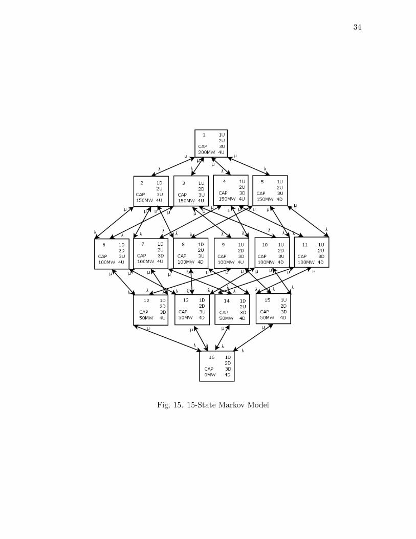
34

Fig. 15. 15-State Markov Model

35

Fig. 16. 5-State Updated Model

ent capacity states. The probabilities of a generator to be up or down is given by:

PUP =µ

λ + µ(4.1)

PDN =λ

λ + µ(4.2)

(4.3)

Hence, the exact probabilities of each capacity level in terms of capacity outages are

given by:

p1 = p(CapOut = 0) =µ4

(λ + µ)4(4.4)

p2 = p(CapOut = 50) =4µ3λ

(λ + µ)4(4.5)

p3 = p(CapOut = 100) =6µ2λ2

(λ + µ)4(4.6)

p4 = p(CapOut = 150) =4µλ3

(λ + µ)4(4.7)

p5 = p(CapOut = 200) =λ4

(λ + µ)4(4.8)

Combining the equivalent states of each capacity level, the number of states are

reduced from 15 to 5. The transition rates between the states are updated accord-

ingly. Figure 16 gives the reduced model with updated transition rates between each

capacity level. The cumulative probabilities for each state is given by:

36

P5 = P (CapOut >= 200) = p5 =λ4

(λ + µ)4(4.9)

P4 = P (CapOut >= 150) = P5 + p4 =λ4 + 4µλ3

(λ + µ)4(4.10)

P3 = P (CapOut >= 100) = P4 + p3 =λ4 + 4µλ3 + 6µ2λ2

(λ + µ)4(4.11)

P2 = P (CapOut >= 50) = P3 + p2 =λ4 + 4µλ3 + 6µ2λ2 + 4µ3λ

(λ + µ)4(4.12)

P1 = P (CapOut >= 0) = P2 + p1 =(λ4 + µ)4

(λ + µ)4= 1 (4.13)

Computation of Cumulative Frequencies:

F1 = p(CapOut >= 0) = 0 (4.14)

F2 = p(CapOut >= 50) = p2µ =4µ4λ

(λ + µ)4(4.15)

F3 = p(CapOut >= 100) = p3(2µ) =12µ3λ2

(λ + µ)4(4.16)

F4 = p(CapOut >= 150) = p4(3µ) =12µ2λ3

(λ + µ)4(4.17)

F5 = p(CapOut >= 200) = p5(4µ) =4µλ4

(λ + µ)4(4.18)

Based on the hourly load data, a load cycle from 0 MW to 151 MW can be developed

with discrete load level steps of 50 MW. For the discrete load levels, Lk:

P (Lk) =Number of Hours where Load Capacity >= Lk

Total Hours in the Interval(4.19)

F (Lk) =No. of transitions from Load < Lk to Load >= Lk

Total Hours in the Interval(4.20)

where P (Lk) and F (Lk) are the probability and frequency of load greater than or equal

to Lk MW. Tables II and III give the probabilities and frequencies of the capacity

states generated from the generation system model and the load model.

37

Table II. Generation System Model Indices

Ck : Outage Level Pk : Prob.of Outage >= Ck Fk : Freq of Outage >= Ck

C1 =0MW P1 =1 F1 = 0

C2 =50MW P2 =0.317 F2 = 0.0114/hr

C3 =100MW P3 =0.044 F3 = 0.0034/hr

C4 =150MW P4 =0.003 F4 = 0.0003/hr

C5 =200MW P5 =0.00007 F5 = 0.0000114/hr

Table III. Load Model Indices

Lk : Load Level Pk : Prob.of Load >= Lk Fk : Freq of Transition from

< Lk to >= Lk

L1 =0MW P1 =1 F1 = 0

L2 =50MW P2 =0.5 F2 = 0.04167/hr

L3 =100MW P3 =0.5 F3 = 0.04167/hr

L4 =150MW P4 =0.167 F4 = 0.04167/hr

38

Table IV. Margin Availability between Load Demand and Generation Capacity Levels

State Cap In Load Level Load Level Load Level Load Level

Levels of 150MW of 100MW of 50MW of 0MW

1 200MW 50 100 150 200

2 150MW 0 50 100 150

3 100MW -50 0 50 100

4 50MW -100 -50 0 50

5 0MW -150 -100 -50 0

Using the theory of Generation Reserve Model [12], the load demand and gener-

ation capacities can be combined to evaluate the margin between capacity generated

versus load demand. A zero margin represents the state where load demand is ex-

actly satisfied by generation. Above this margin load demand is satisfied and there is

surplus generation, while below this margin loss of load occurs. The reliability indices

HLOLE and FLOL can be computed using this technique. Table IV gives all possible

margins for each state between capacity available and load demand.

Using the values from Table IV the probability and frequency of zero margin

can be evaluated. HLOLE index is obtained from the product of this probability

and number of hours in a year. The frequency of zero margin transition occurs from

generation capacity changes as well as changes in the load cycle. FLOL is the sum

of these two frequencies. System HLOLE is computed to be 591.23 hrs/yr. System

FLOL value is 0.01625/hr.

39

Source

0

GEN1 GEN2 GEN3 GEN4

Sink

LOAD

Fig. 17. Small System Graph Simulation

2. Developed Simulation Methodology

The reliability indices of the same network are computed and validated using the

Monte Carlo-Max Flow based methodology developed in this thesis. The failure

and repair history of the generators is created using using random variables with

exponential distribution. Figure 17 shows the graphical view of the network flow for

this system.

Based on convergence criterion of COV of 2.5 for the system HLOLE, the relia-

bility indices are computed to be

1. System HLOLE of 591.14 hrs/yr

2. System FLOL of 142.25/yr or 0.01624/hr

40

Fig. 18. Distribution System for RBTS BUS 2

C. Distribution System Data

Two types of networks used for the case studies are shown in Figure 18 and 19. These

are distribution systems connected to bus 2 and bus 4 of the RBTS [14] modified for

DG analysis. Transformers and breakers are not included in the analysis. Both

networks are configured to have two main supply points, each of capacity equal to

half of the total energy supplied to the network.

For the analysis, different capacity levels for the supply points are considered. In

addition, DG is included at various points in the networks. The network points with

41

Fig. 19. Distribution System for RBTS BUS 4

loads having the highest indices for HLOLE and EUE are chosen for DG placment.

Some of these cases will be analysed in the next chapter. The load points with lower

reliability indices usually occur in the end of the feeders, farthest from the supply

points.

1. Distributions for Component Models

For both the networks, the supply point failure rates and mean repair times are

4.42 failures/year and 20 hours respectively. Distribution line failure rates and mean

repair times are 0.44 failures/year and 10 hours respectively. DG is modeled in

the same manner as the main supply with the same failure rates and repair times.

42

The mean Time-To-Failure (TTF) for the generation and lines are assumed to have

exponential distribution. The mean Time-To-Repair (TTR) for the generation and

lines are assumed to have log-normal distribution. The relation between the transition

times and transition rates is given by

λ =1

TTF(4.21)

µ =1

TTR(4.22)

Exponential distributions have cumulative distribution functions of the form:

P (X <= x) = Fx (x) = 1− e−ρx; (4.23)

with mean 1ρ.

For simulation using Monte Carlo methods, it is useful to generate random num-

bers from an exponential distribution. For example, it is a standard practice to model

a component’s TTF using an exponential distribution, especially when rate of failure

is assumed to be relatively constant (no aging). Generally, most software languages

provide a floating-point random number generator that is uniform on [0, 1). For a

random number z taken from a uniform distribution on [0, 1), a realization of an

exponentially distributed random variable X with parameter ρ can be obtained by :

x = − ln (z)

ρ(4.24)

Similarly, it is a commonly believed that a log-normal distribution is a good

representation of repair time. Log-normal distributions with parameters (M, S) are

defined by:

P (X = x) =1

S√

2πxe−

(ln(x)−M)2

2S2 (4.25)

43

mean = eM+S2

2 (4.26)

variance = eS2+2M(eS2 − 1

)(4.27)

A variety of techniques exist [15] for computing realizations of a normal distri-

bution using a uniform random number generator. Furthermore, a realization, x, of

a log-normal distribution with parameters (M, S) can be obtained from a realization,

z, of a standard normal distribution by computing:

x = eM+Sz (4.28)

2. Load Models

The different load categories and classifications are obtained from the RBTS network

data [14]. Bus 2 has four types of customers viz. residential, small user, govern-

ment/institution and commercial. Bus 4 has three types of customers viz. residential,

small user and commercial. All the load points of the two networks are classified as

one of these customer types. The total peak load for Bus 2 is 20 MW, while the total

peak for Bus 4 is 40 MW.

For the load modeling, hourly time-varying characteristics is incorporated. The

weekly loads for 52 weeks are expressed as percentages of the annual peak load for

the different customer types mentioned above. Figure 20 gives the load cycle for all

the weeks in a year. An electric utility data [16] is used for the percent weekly, daily

and hourly values.

Figure 21 gives the daily loads for seven days as percentages of the weekly peak.

Finally, the hourly load data as percentages of the daily peak as weekday or week-

end for summer, winter and spring/fall weeks as shown in Figures 22, 24 and 23

respectively.

44

0

10

20

30

40

50

60

70

80

90

100

1 3 5 7 9 11 13 15 17 19 21 23 25 27 29 31 33 35 37 39 41 43 45 47 49 51

Week

Wee

kly

Pea

k

Fig. 20. Weekly Load as Percent of Annual Peak

0

10

20

30

40

50

60

70

80

90

100

Monday Tuesday Wednesday Thursday Friday Saturday Sunday

Day

Dai

ly P

eak

Fig. 21. Daily Load as Percent of Weekly Peak

45

0

10

20

30

40

50

60

70

80

90

100

0 1 2 3 4 5 6 7 8 9 10 11 12 13 14 15 16 17 18 19 20 21 22 23

Hour of Day

Hourly Peak

Weekday

Weekend

Fig. 22. Hourly Load as Percent of Daily Peak in Summer Weeks

0

10

20

30

40

50

60

70

80

90

100

0 1 2 3 4 5 6 7 8 9 10 11 12 13 14 15 16 17 18 19 20 21 22 23

Hour of Day

Hourly Peak

Weekday

Weekend

Fig. 23. Hourly Load as Percent of Daily Peak in Spring/Fall Weeks

46

0

10

20

30

40

50

60

70

80

90

100

0 1 2 3 4 5 6 7 8 9 10 11 12 13 14 15 16 17 18 19 20 21 22 23

Hour of Day

Hourly Peak

Weekday

Weekend

Fig. 24. Hourly Load as Percent of Daily Peak in Winter Weeks

47

CHAPTER V

CASE STUDIES

A wide range of scenarios are simulated and studied to assess the reliability of the

modified distribution networks of the RBTS Bus 2 and Bus 4 described in the previous

chapter. Using the Monte Carlo-Max Flow methodology, distributions for component

models and time varying load characteristics described in the earlier chapters, the

networks are simulated and various reliability indices are evaluated.

A. BUS 2 Reliability Results

The first study considers the Bus 2 network. This network has 4 feeders, 36 distribu-

tion lines and 22 load points. A statistic for convergence, COV, described in chapter

III is maintained. At each simulated year, the coefficient of variation of the system-

wide HLOLE is sampled and a running mean and standard deviation are updated.

The system level statistics for all the cases are recorded when the sampled HLOLE

reaches a COV of 2.5. However, in order to compare the individual load point indices,

convergence of system HLOLE doesn’t necessarily imply convergence of load point

statistics. This is due to the fact that the system converges faster than the individual

load points. Hence, a convergence criterion based on the load point EUE index is

used for collecting load statistics and for comparing the specific load status. A COV

of 2.5 gives a 95 percent confidence margin for the obtained statistics.

The graphical illustration for all these cases represent the actual distribution

network links with added nodes to show the interconnections between distribution

lines, supply points and loads. Lines in blue indexed G01 etc represent generation

supply arcs, lines in brown indexed T01, T02 etc represent distribution arcs and green

lines represent load points indexed as L01, L02 etc. DG arcs are also represented by

48

blue line but with index DG01, DG02 etc. To run the Max-Flow module all generation

arcs including DG arcs are connected to the source node and all load arcs terminate

into the sink node. The nodes into which DG arcs terminate represent the actual

placement location for the DG.

1. Supply Capacity of 20 MW

In this case, the total supply capacity is assumed to be 20 MW, which is exactly

equal to the maximum peak load. Two generators with identical failure and repair

characteristics, each of capacity 10 MW, are used to represent the supply points to the

distribution network. Loss of load may occur from either generation or line outage.

For this particular case, outage of any one of the generators reduces the system supply

to 10 MW or half the peak load demand. Hence, loss of load occurs frequently since

there is no redundancy in the total generation supply.

The graphical flow overview for the simulated network for the base case is shown

in Figure 25. The reliability indices are divided into two categories; system level

indices and individual load point indices. The system EUE index is the sum of all the

individual load point EUE indices. However, the system HLOLE is not the sum of the

load point HLOLE. Any instance of loss of load in the network counts as one instance

of system loss of load irrespective of the number of load points unsupplied. Hence,

one load point unsupplied or multiple load points unsupplied at the same instance of

time are equivalent where system HLOLE is concerned.

The load point indices, HLOLE and EUE are the worst at the end of feeder

locations since these loads are supplied from the longest chains of distribution lines,

the failure rates of which add up. A good choice for DG placement should improve

the load point reliability of such loads. In the next case, 1 DG is added as standby

supply at node 9 of the Bus 2 network and simulated as shown in Figure 26. This

49

Source

2

G01 G02

Sink

3

T01

14

T12

18

T16

28

T26

6

T04

4

T02

5

T039

T07

7

T05

8

T06

12

T10

10

T08

11

T09

13

T11

16

T14

15

T13

17

T15

20

T18

19

T1723

T21

21

T19

22

T20

26

T24

24

T22

25

T23

27

T25

31

T29

30

T28

29

T2734

T32

32

T30

33

T31

36

T34

35

T33

37

T35

38

T36

L01 L02L03 L10L11 L12 L17L18 L19L08L09L04L05 L13 L14 L20L21L06L07 L15 L16L22

Fig. 25. Bus 2 Network with Supply of 20 MW

Source

2

G01 G02

9

DG01

Sink

3

T01

14

T12

18

T16

28

T26

6

T04

4

T02

5

T03

T07

7

T05

8

T06

12

T10

10

T08

11

T09

13

T11

16

T14

15

T13

17

T15

20

T18

19

T17 23

T21

21

T19

22

T20

26

T24

24

T22

25

T23

27

T25

31

T29

30

T28

29

T27 34

T32

32

T30

33

T31

36

T34

35

T33

37

T35

38

T36

L01 L02 L03L10 L11L12 L17 L18L19L08L09 L04 L05L13L14 L20L21 L06L07L15 L16 L22

Fig. 26. Bus 2 Network with Supply of 20 MW and 1 DG

50

Source

2

G01 G02

9

DG01

34

DG02

Sink

3

T01

14

T12

18

T16

28

T26

6

T04

4

T02

5

T03

T07

7

T05

8

T06

12

T10

10

T08

11

T09

13

T11

16

T14

15

T13

17

T15

20

T18

19

T17 23

T21

21

T19

22

T20

26

T24

24

T22

25

T23

27

T25

31

T29

30

T28

29

T27

T32

32

T30

33

T31

36

T34

35

T33

37

T35

38

T36

L01 L02 L03 L10 L11 L12 L17 L18 L19L08 L09L04 L05 L13 L14 L20 L21L06 L07 L15 L16 L22


Table V. Comparison of System Level Indices for Bus 2 Supply of 20 MW

Reliability Index No DG 1 DG 2 DG

EUE 966.47 661.29 352.10

HLOLE 408.31 380.85 299.76

FLOL 31.1 31.1 28.2

51

node is located near the end of Feeder 1 and supplies load points 5, 6 and 7 in the

event of system generation outage or failure of lines upstream that would feed these

loads. In the base case, these loads have significantly higher HLOLE and EUE. The

DG capacity is 3 MW which is slighly higher than the sum of demands of the three

load points. In addition to improving the individual indices for load points directly

fed by the DG, the system level statistics show significant improvement. The next

case studies the same network with 2 DG connected at nodes 9 and 34 respectively

as shown in Figure 27. The DG at node 34 offers standby support to load points 20,

21 and 22. Table V gives the system level EUE, HLOLE and FLOL indices for Bus

2 network at generation of 20 MW. The base case is compared with the cases where

1 and 2 DG are added. The EUE index shows the most significant improvement and

is the best index of assessment. Figure 28 compares the load point EUE for all 22

loads in the network for the three cases.At some load points where the EUE index

is very low to begin with,addition of DG doesn’t cause much difference. The load

points directly benefitting from DG show significant drop in EUE. In the event of

any system generation outage, the available generation can be assigned to the loads

where DG is not connected, thereby improving the reliability of loads that originally

experienced high loss.


In power networks, it is common practice to have some margin between the supply

and maximum load demand. Hence, in the cases considered in this section, the total

supply capacity is assumed to be 30 MW. Each of the two equivalent generators now

supply 5 MW more than the previous case. It is probable that in the event of loss of

any one generation, the load demand may still be met by the standing generation of

15 MW as long as the minimum load demand in its time varying cycle is not above 15

52

0

20

40

60

80

100

120

140

L01 L02 L03 L04 L05 L06 L07 L08 L09 L10 L11 L12 L13 L14 L15 L16 L17 L18 L19 L20 L21 L22

Load Points

EU

E (

MW

hr/

yr)

EUE (mean) DG0EUE (mean) DG1EUE (mean) DG2

Fig. 28. Load Point EUE Indices for Bus 2 Supply of 20 MW

53

Source

2

G01 G02

Sink

3

T01

14

T12

18

T16

28

T26

6

T04

4

T02

5

T039

T07

7

T05

8

T06

12

T10

10

T08

11

T09

13

T11

16

T14

15

T13

17

T15

20

T18

19

T1723

T21

21

T19

22

T20

26

T24

24

T22

25

T23

27

T25

31

T29

30

T28

29

T2734

T32

32

T30

33

T31

36

T34

35

T33

37

T35

38

T36



MW. Also, with the surplus generation, the line failure rates have greater influence

on the loss of load and unserved energy indices. This is not true in the previous

section when the supply, when fully available, exactly satisfied the demand and the

generation failure rate being significantly greater than line failure rate, dictated the

status of the load.

Figures 29, 30, 31 show the graphical overview of the distribution network at

supply capacity of 30 MW for the base case, for 1 DG added at node 9 and for 2

DG added node 9 and 34 of the network respectively. For the three cases, Table VI

compares the EUE, HLOLE and FLOL indices. Firstly, it is observed that for the

base case, EUE index is about a third of the previous base case due to surplus supply.

The HLOLE and FLOL indices are reduced as well. However, the addition of DG

result in comparable reductions in system EUE and HLOLE indices.

54

Source

2

G01 G02

9

DG01

Sink

3

T01

14

T12

18

T16

28

T26

6

T04

4

T02

5

T03

T07

7

T05

8

T06

12

T10

10

T08

11

T09

13

T11

16

T14

15

T13

17

T15

20

T18

19

T17 23

T21

21

T19

22

T20

26

T24

24

T22

25

T23

27

T25

31

T29

30

T28

29

T27 34

T32

32

T30

33

T31

36

T34

35

T33

37

T35

38

T36



Source

2

G01 G02

9

DG01

34

DG02

Sink

3

T01

14

T12

18

T16

28

T26

6

T04

4

T02

5

T03

T07

7

T05

8

T06

12

T10

10

T08

11

T09

13

T11

16

T14

15

T13

17

T15

20

T18

19

T17 23

T21

21

T19

22

T20

26

T24

24

T22

25

T23

27

T25

31

T29

30

T28

29

T27

T32

32

T30

33

T31

36

T34

35

T33

37

T35

38

T36



55

Table VI. Comparison of System Level Indices for Bus 2 Supply of 30 MW


EUE 316.98 245.21 205.69

HLOLE 261.78 214.85 198.44

FLOL 23.7 17.6 14.8

0

5

10

15

20

25

30

35

40


Load Points

EU

E (

MW

hr/

yr)


Fig. 32. Load Point EUE Indices for Bus 2 Supply 30 MW

56

The differences in the load point EUE for the three cases is recorded in Figure

32. The load point EUE values are significantly lower than those in the previous

section. Loads directly served by the DG, in the event of supply outage, show similar

improvements from the base case as seen in the previous section. However, for all

other loads that experienced the most outage, addition of DG does not produce much

difference. This is again due to the fact that generation outage is a less influencing

factor than line outage when there is surplus generation. Hence, for loads that are not

directly fed from DG, loss of load is caused more often by line outage than generation

outage and the reliability indices stand unaffected.


The final case for the Bus 2 distribution network considers supply of 40 MW. The two

equivalent generators each supplying 20 MW are individually capable of handling the

maximum load demand of the entire network. Hence, loss of one generator will never

result in loss of load in the network even if the load demand at that instance is the

maximum in the cycle. Loss of load can only occur in the event that both generators

are in outage or any distribution line is failed.

Figures 33, 34, 35 illustrate the simulated network state with Supply of 40 MW in

the base case and with 1 and 2 DG added to it. Table VII gives the comparison of the

reliability indices for the three cases. The significant difference from the previous cases

is seen in the system indices. Although, the addition of DG causes some lowering in

these indices, the improvement is significantly less than that in the previous sections.

Comparison of individual load point EUE values given in Figure 36 shows DG to still

have positive effect on the load points directly supplied from it. However, for all other

cases, the individual load point indices have no correlation with the presence of the

DG since the capacity of DG is negligible compared to the high surplus of the Supply.

57

Source

2

G01 G02

Sink

3

T01

14

T12

18

T16

28

T26

6

T04

4

T02

5

T039

T07

7

T05

8

T06

12

T10

10

T08

11

T09

13

T11

16

T14

15

T13

17

T15

20

T18

19

T1723

T21

21

T19

22

T20

26

T24

24

T22

25

T23

27

T25

31

T29

30

T28

29

T2734

T32

32

T30

33

T31

36

T34

35

T33

37

T35

38

T36



Source

2

G01 G02

9

DG01

Sink

3

T01

14

T12

18

T16

28

T26

6

T04

4

T02

5

T03

T07

7

T05

8

T06

12

T10

10

T08

11

T09

13

T11

16

T14

15

T13

17

T15

20

T18

19

T17 23

T21

21

T19

22

T20

26

T24

24

T22

25

T23

27

T25

31

T29

30

T28

29

T27 34

T32

32

T30

33

T31

36

T34

35

T33

37

T35

38

T36



58

Source

2

G01 G02

9

DG01

34

DG02

Sink

3

T01

14

T12

18

T16

28

T26

6

T04

4

T02

5

T03

T07

7

T05

8

T06

12

T10

10

T08

11

T09

13

T11

16

T14

15

T13

17

T15

20

T18

19

T17 23

T21

21

T19

22

T20

26

T24

24

T22

25

T23

27

T25

31

T29

30

T28

29

T27

T32

32

T30

33

T31

36

T34

35

T33

37

T35

38

T36



Also, the failure rate of the DG is now greater than the rate of overlapping failure of

the two system generators. Hence, in such a case, other that small improvement to

directly connected load points, addition of DG has no positive effect to the distribution

network.

59

Table VII. Comparison of System Level Indices for Bus 2 Supply of 40 MW


EUE 267.89 250.06 197.88

HLOLE 213.73 207.26 197.21

FLOL 15.7 15.3 14.5

0

5

10

15

20

25


Load Points

EU

E (

MW

hr/

yr)



60

B. BUS 4 Reliability Results

The distribution system of the RBTS Bus 4 is also evaluated by the developed method-

ology. Some modifications are made to the network as described in the previous chap-

ter. Different capacity levels for supply are considered in a similar fashion to the Bus

2 network. Bus 4 is a larger network than Bus 2 with 7 feeders, 67 distribution lines

and 38 loads. For more details of the networks please refer to the previous chapter.


The maximum system load demand for this network is 40 MW. The first study as-

sumes the supply capacity to be exactly equal to this maximum demand. The system

supply is represented by two generators each of capacity half of the total supply.

Hence, loss of load occurs when any one of the generators or lines are failed. The

generator failure rate assumed to be ten times the line failure rate has the greatest

influence on the status of load satisfaction. Figure 37 gives the graphical overview of

the simulated network.

61

Source

2

G01 G02

Sink

3

T01

15

T13

21

T19

33

T31

46

T44

52

T50

58

T56

5

T03

4

T02

7

T05

6

T049

T07

8

T06

12

T10

10

T08

11

T09

13

T11

14

T12

17

T15

16

T14

19

T17

18

T16

20

T18

23

T21

22

T20

25

T23

24

T2228

T26

26

T24

27

T25

30

T28

29

T27

32

T30

31

T29

35

T33

34

T32

38

T36

36

T34

37

T3541

T39

39

T37

40

T38

43

T41

42

T40

44

T42

45

T43

48

T46

47

T45

50

T48

49

T47

51

T49

54

T52

53

T51

56

T54

55

T53

57

T55

60

T58

59

T57

62

T60

61

T5965

T63

63

T61

64

T62

67

T65

66

T64

68

T66

69

T67

L01L02L03L04 L11L12L13 L18L19 L20L21 L32L33L34 L35L05 L14L15 L22L23 L36L37L08L10 L26L27L28 L29L30L09 L31L06 L07 L16 L17 L24 L25 L38


61

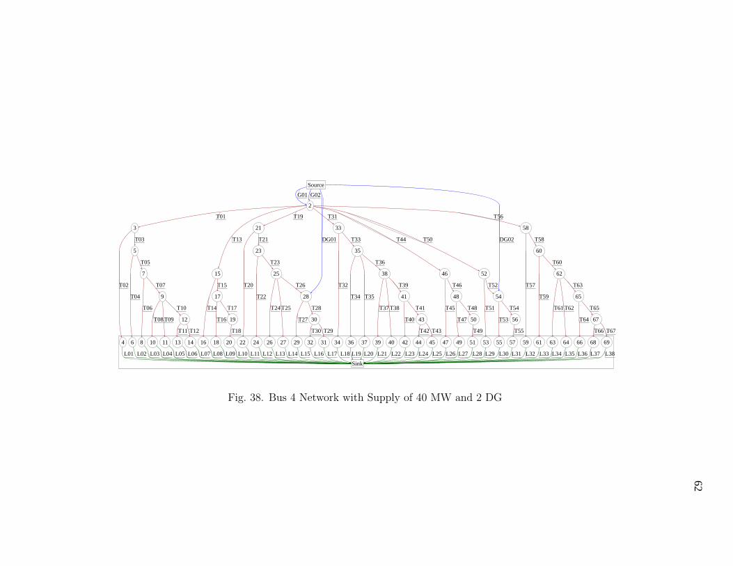
62

Source

2

G01 G02

28

DG01

54

DG02

Sink

3

T01

15

T13

21

T19

33

T31

46

T44

52

T50

58

T56

5

T03

4

T02

7

T05

6

T04 9

T07

8

T06

12

T10

10

T08

11

T09

13

T11

14

T12

17

T15

16

T14

19

T17

18

T16

20

T18

23

T21

22

T20

25

T23

24

T22

T26

26

T24

27

T25

30

T28

29

T27

32

T30

31

T29

35

T33

34

T32

38

T36

36

T34

37

T35 41

T39

39

T37

40

T38

43

T41

42

T40

44

T42

45

T43

48

T46

47

T45

50

T48

49

T47

51

T49

T52

53

T51

56

T54

55

T53

57

T55

60

T58

59

T57

62

T60

61

T59 65

T63

63

T61

64

T62

67

T65

66

T64

68

T66

69

T67

L01 L02 L03 L04 L11 L12 L13 L18 L19 L20 L21 L32 L33 L34 L35L05 L14 L15 L22 L23 L36 L37L08 L10 L26 L27 L28 L29 L30L09 L31L06 L07 L16 L17 L24 L25 L38


62

63

Source

2

G01 G02

28

DG01

41

DG03

54

DG02

65

DG04

Sink

3

T01

15

T13

21

T19

33

T31

46

T44

52

T50

58

T56

5

T03

4

T02

7

T05

6

T04 9

T07

8

T06

12

T10

10

T08

11

T09

13

T11

14

T12

17

T15

16

T14

19

T17

18

T16

20

T18

23

T21

22

T20

25

T23

24

T22

T26

26

T24

27

T25

30

T28

29

T27

32

T30

31

T29

35

T33

34

T32

38

T36

36

T34

37

T35

T39

39

T37

40

T38

43

T41

42

T40

44

T42

45

T43

48

T46

47

T45

50

T48

49

T47

51

T49

T52

53

T51

56

T54

55

T53

57

T55

60

T58

59

T57

62

T60

61

T59

T63

63

T61

64

T62

67

T65

66

T64

68

T66

69

T67



63

64

Table VIII. Comparison of System Level Indices for Bus 4 Supply of 40 MW


EUE 2107.32 1197.13 682.15

HLOLE 598.04 519.95 461.56

FLOL 43.8 41.69 39.2

The load points at the end of the feeders that have the most number of distri-

bution arcs show the highest indices for EUE and HLOLE. Hence, DG operating in

standby mode is added to the network to assess the system reliability. First case

considers addition of 2 DG at nodes 28 and 54. These nodes connect the load points

farthest from the supply. In addition, node 54 is connected to loads that have the

highest individual peak load of the entire network. Hence, these load points experi-

ence much higher loss of load than others. Installed DG at node 28 will offer standby

support to loads 15, 16 and 17 and DG at node 54 supplies to loads 30 and 31. The

capacity of the DG at node 28 is 2.5 MW and the capacity of the DG at node 54 is

4.1 MW. These values are the sum of the peak demand of the supplied load points.

Figure 38 shows the flow network of the Bus 4 distribution network with 2 DG.

Since the network is large, there are several load points which experience sub-

stantially high outage indices. Hence, the final case considers addition of 4 DG to

the network. As in the previous case, there are 2 DG each at node 28 and 54 as well

as a DG at nodes 41 and 65 of capacity 2.5 MW. Node 41 connects to load points

23, 24 and 25 and node 65 connects to load points 36, 37 and 38 as shown in Figure

39. Comparison of system reliability indices in Table VIII show marked improvement

when 2 and 4 DG are added. In this case, where outage of any one of the system

generators result in loss of load, the load point EUE significantly improve on addition

65

0

20

40

60

80

100

120

140

L01 L03 L05 L07 L09 L11 L13 L15 L17 L19 L21 L23 L25 L27 L29 L31 L33 L35 L37

Load Points

EU

E (

MW

hr/

yr)



66

of DG. All load points, whether they are supplied by the DG or not show significantly

reduced EUE in Figure 40. This again is attributed to the fact that limited available

generation is fed to loads not connected to DG which is a lesser number than the

number of loads to be supplied during partial generation outage and no DG. Hence,

reliability of all load points are improved with addition of DG when the supply outage

is the main factor for loss of load.


The next case considers the Bus 4 network with an increased supply capacity of 60

MW. The two generators now supply 30 MW each. If the minimum point in the

system load cycle is less than 30 MW, then outage of any one of the generators does

not result in loss of load.

67

Source

2

G01 G02

Sink

3

T01

15

T13

21

T19

33

T31

46

T44

52

T50

58

T56

5

T03

4

T02

7

T05

6

T049

T07

8

T06

12

T10

10

T08

11

T09

13

T11

14

T12

17

T15

16

T14

19

T17

18

T16

20

T18

23

T21

22

T20

25

T23

24

T2228

T26

26

T24

27

T25

30

T28

29

T27

32

T30

31

T29

35

T33

34

T32

38

T36

36

T34

37

T3541

T39

39

T37

40

T38

43

T41

42

T40

44

T42

45

T43

48

T46

47

T45

50

T48

49

T47

51

T49

54

T52

53

T51

56

T54

55

T53

57

T55

60

T58

59

T57

62

T60

61

T5965

T63

63

T61

64

T62

67

T65

66

T64

68

T66

69

T67



67

68

Source

2

G01 G02

28

DG01

54

DG02

Sink

3

T01

15

T13

21

T19

33

T31

46

T44

52

T50

58

T56

5

T03

4

T02

7

T05

6

T04 9

T07

8

T06

12

T10

10

T08

11

T09

13

T11

14

T12

17

T15

16

T14

19

T17

18

T16

20

T18

23

T21

22

T20

25

T23

24

T22

T26

26

T24

27

T25

30

T28

29

T27

32

T30

31

T29

35

T33

34

T32

38

T36

36

T34

37

T35 41

T39

39

T37

40

T38

43

T41

42

T40

44

T42

45

T43

48

T46

47

T45

50

T48

49

T47

51

T49

T52

53

T51

56

T54

55

T53

57

T55

60

T58

59

T57

62

T60

61

T59 65

T63

63

T61

64

T62

67

T65

66

T64

68

T66

69

T67



68

69

Source

2

G01 G02

28

DG01

41

DG03

54

DG02

65

DG04

Sink

3

T01

15

T13

21

T19

33

T31

46

T44

52

T50

58

T56

5

T03

4

T02

7

T05

6

T04 9

T07

8

T06

12

T10

10

T08

11

T09

13

T11

14

T12

17

T15

16

T14

19

T17

18

T16

20

T18

23

T21

22

T20

25

T23

24

T22

T26

26

T24

27

T25

30

T28

29

T27

32

T30

31

T29

35

T33

34

T32

38

T36

36

T34

37

T35

T39

39

T37

40

T38

43

T41

42

T40

44

T42

45

T43

48

T46

47

T45

50

T48

49

T47

51

T49

T52

53

T51

56

T54

55

T53

57

T55

60

T58

59

T57

62

T60

61

T59

T63

63

T61

64

T62

67

T65

66

T64

68

T66

69

T67



69

70

Table IX. Comparison of System Level Indices for Bus 4 Supply of 60 MW


EUE 700.64 587.81 453.17

HLOLE 431.99 392.79 362.15

FLOL 35.5 29.5 27.5

Figures 41, 42, 43 show the graphical flow networks for the base case, 2 DG added

and 4 DG added to the network at the same nodes as the previous cases. Table IX

compares the reliability indices for no DG, 2 DG and 4 DG in the Bus 4 distribution

network. As observed in the Bus 2 cases, the EUE index shows significant reduction

from the lower generation case. The addition of DG improves the indices in the same

manner as in the case of Supply of 40 MW. For the load point reliability indices, the

loads directly supplied from the DG show improvement in unserved energy. This is

demonstrated in Figure 44.


Finally, the last case for the Bus 4 network considers the capacity of supply to be

double the maximum system load. Irrespective of the magnitude of load, any one of

the two generators is capable of supplying the entire system load. Loss of load due to

generation occurs only when both system generators are in outage in the same time.

71

0

5

10

15

20

25

30

35

40

45


Load Points

EU

E (

MW

hr/

yr)



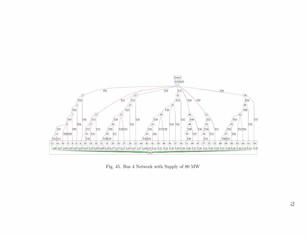
72

Source

2

G01 G02

Sink

3

T01

15

T13

21

T19

33

T31

46

T44

52

T50

58

T56

5

T03

4

T02

7

T05

6

T049

T07

8

T06

12

T10

10

T08

11

T09

13

T11

14

T12

17

T15

16

T14

19

T17

18

T16

20

T18

23

T21

22

T20

25

T23

24

T2228

T26

26

T24

27

T25

30

T28

29

T27

32

T30

31

T29

35

T33

34

T32

38

T36

36

T34

37

T3541

T39

39

T37

40

T38

43

T41

42

T40

44

T42

45

T43

48

T46

47

T45

50

T48

49

T47

51

T49

54

T52

53

T51

56

T54

55

T53

57

T55

60

T58

59

T57

62

T60

61

T5965

T63

63

T61

64

T62

67

T65

66

T64

68

T66

69

T67



72

73

Source

2

G01 G02

28

DG01

54

DG02

Sink

3

T01

15

T13

21

T19

33

T31

46

T44

52

T50

58

T56

5

T03

4

T02

7

T05

6

T04 9

T07

8

T06

12

T10

10

T08

11

T09

13

T11

14

T12

17

T15

16

T14

19

T17

18

T16

20

T18

23

T21

22

T20

25

T23

24

T22

T26

26

T24

27

T25

30

T28

29

T27

32

T30

31

T29

35

T33

34

T32

38

T36

36

T34

37

T35 41

T39

39

T37

40

T38

43

T41

42

T40

44

T42

45

T43

48

T46

47

T45

50

T48

49

T47

51

T49

T52

53

T51

56

T54

55

T53

57

T55

60

T58

59

T57

62

T60

61

T59 65

T63

63

T61

64

T62

67

T65

66

T64

68

T66

69

T67



73

74

Source

2

G01 G02

28

DG01

41

DG03

54

DG02

65

DG04

Sink

3

T01

15

T13

21

T19

33

T31

46

T44

52

T50

58

T56

5

T03

4

T02

7

T05

6

T04 9

T07

8

T06

12

T10

10

T08

11

T09

13

T11

14

T12

17

T15

16

T14

19

T17

18

T16

20

T18

23

T21

22

T20

25

T23

24

T22

T26

26

T24

27

T25

30

T28

29

T27

32

T30

31

T29

35

T33

34

T32

38

T36

36

T34

37

T35

T39

39

T37

40

T38

43

T41

42

T40

44

T42

45

T43

48

T46

47

T45

50

T48

49

T47

51

T49

T52

53

T51

56

T54

55

T53

57

T55

60

T58

59

T57

62

T60

61

T59

T63

63

T61

64

T62

67

T65

66

T64

68

T66

69

T67



74

75

Table X. Comparison of System Level Indices for Bus 4 Supply of 80 MW


EUE 562.22 555.38 478.33

HLOLE 383.04 373.53 371.58

FLOL 28.3 27.7 27.4

Figures 45, 46, 47 show the graphical flow networks for the base case, 2 DG

added and 4 DG added to the network. Comparison of the system reliability indices

in Table X show relatively low improvement on the already reduced indices by adding

DG to the network. This is also demonstrated in the trend of the load point EUE

for the three cases in Figure 48. Since there already exists a large redundancy in the

supply capacity as opposed to the load demand, the combined input of the DG is

negligible to impact the load indices with the exception of loads directly fed by DG

when both system generators or upstream line fail.

In conclusion, analysis of the two different distribution networks validates general

reliability assessments for load points and overall system. EUE is shown to be the

most sensitive index of reliablity and the relative influence of DG in a network is

seen be closely related to the capacity redundancy of the supply. Loads connected to

DG always demonstrate improved reliability, however the improvement of other load

point reliability indices depend on whether the generation outage or line outage is

the principle contributor for loss of load.

76

0

5

10

15

20

25

30

35

40

45


Load Points

EU

E (

MW

hr/

yr)



77

CHAPTER VI

CONCLUSIONS

This research has presented a new methodology that can simulate the operation of

a distribution network with Distributed Generation and evaluate the status of load

demand and system reliability in such a network. The methodology combines a

sequential Montel Carlo simulation of the system’s stochastic model states with a

path augmenting Max flow algorithm to determine the status of load demand in the

system and to generate reliability statistics at the system and load point levels.

A flexible and efficient simulator has been developed in C++ to implement this

methodology. Various additional features such as multiple distributions for the supply

and distribution line outage and repair rates and time-varying load characteristics

have been incorporated. Further, techniques to enhance the performance of this

computation-intensive simulation have also been discussed.

Cases of different supply level distribution networks with variable number of DG

have been studied to analyze the reliability impact of DG to the network at system

level and at specific load points. The reliability assessment is based on computation

of indices such as HLOLE, FLOL and EUE.

Based on the results, EUE is observed to be the most responsive index of reliablity

for this application. Also, the relative impact of DG in a network is seen be related to

the capacity redundancy of the supply in the network. Loads connected to DG always

demonstrate improved reliability. Elsewhere in the network DG enhanced reliability

to a lesser degree by reducing the feeder loadings. However, the improvement of these

load point reliability indices depends on whether the generation outage or line outage

is the principle contributor for loss of load. Further research on this aspect can be

done to device a new index of reliability for a distribution network with DG.

78

REFERENCES

[1] A. A. Chowdhury and D. O. Koval, “Generation reliability impacts of industry-

owned distributed generation sources,” in Industry Applications Conference,

vol. 2, Oct. 2003, pp. 1321–1327.

[2] R. Billinton and R. N. Allan, Reliability Evaluation of Power Systems, 2nd ed.

New York: Plenum Press, 1996.

[3] C. Singh and A. Lago-Gonzalez, “Reliability modeling of generation systems in-

cluding unconventional energy sources,” IEEE Transactions on Power Apparatus

and Systems, vol. 104, no. 5, May 1985.

[4] C. Singh and Y. Kim, “An efficient technique for reliability analysis of power sys-

tems including time dependent sources,” IEEE Transactions on Power Systems,

vol. 3, no. 3, pp. 1090–1096, Aug. 1988.

[5] P. Wang and R. Billinton, “Time-sequential simulation techniques for rural dis-

tribution system reliability cost/worth evaluation including wind generation as

alternate supply,” in IEE Proc. Transmission, Distribution, and Generation, vol.

148, no. 4, July 2001, pp. 355–360.

[6] R. E. Brown and L. A. A. Freeman, “Analyzing the reliability impact of dis-

tributed generation,” in IEEE PES Summer Meeting, vol. 2, July 2001, pp.

1013–1018.

[7] J. A. Greatbanks, D. H. Popovic, M. Begovic, A. Pregelj, and T. C. Green,

“On optimization for security and reliability of power systems with distributed

generation,” in Power Tech Conf. Proc., vol. 1, Bologna, Italy, June 2003.

79

[8] A. A. Chowdhury, S. K. Agarwal, and D. Koval, “Reliability modeling of dis-

tributed generation in conventional distribution systems planning and analysis,”

IEEE Transactions on Industry Applications, vol. 39, no. 5, pp. 1493–1498, Sept.-

Oct. 2003.

[9] Y. G. Hegazy, M. M. A. Salama, and A. Y. Chikhani, “Adequacy assessment of

distributed generation systems using Monte Carlo simulation,” IEEE Transac-

tions on Power Systems, vol. 18, no. 1, pp. 48–52, Feb. 2003.

[10] I. S. Bae, J. O. Kim, J. C. Kim, and C. Singh, “Optimal operating strategy for

distributed generation considering hourly reliability worth,” IEEE Transactions

on Power Systems, vol. 19, no. 1, pp. 287–292, Feb. 2004.

[11] R. Billinton and W. Li, Reliability Assessment of Electric Power Systems Using

Monte Carlo Methods. New York: Plenum Press, 1994.

[12] C. Singh, “Electrical power system reliability,” 1995, course notes. [Online].

Available: http://www.ece.tamu.edu/People/bios/singh/coursenotes/

[13] L. R. Ford and D. R. Fulkerson, Flows in Networks. Princeton, NJ: Princeton

University Press, 1962.

[14] R. N. Allan, R. Billinton, I. Sjarief, L. Goel, and K. S. So, “A reliability test sys-

tem for educational purposes-basic distribution system data and results,” IEEE

Transactions on Power Systems, vol. 6, no. 2, pp. 813 – 820, May 1991.

[15] R. E. Odeh and J. O. Evans, “Statistical algorithms: Algorithm AS 70: The

percentage points of the normal distribution,” Applied Statistics, vol. 23, no. 1,

pp. 96–97, Mar. 1974.

80

[16] Y. Li, “Bulk system reliability evaluation in a deregulated power industry,” Mas-

ter’s thesis, University of Saskatchewan, Dec. 2003.

81

APPENDIX A

SIMULATION RESULTS FOR SYSTEM COMPONENTS

Bus 2 and Bus 4 supply points, distributed generators and distribution lines

statistics for hours of outage and frequency of outages per year are recorded in the

following tables.

Table XI. Bus 2 Results, Supply Capacity 20 MW

No DG case 1 DG case 2 DG caseHrs/yr Freq/yr Hrs/yr Freq/yr Hrs/yr Freq/yr

Supply PointsGen01 142.831 4.32176 140.577 4.25853 143.694 4.34766Gen02 141.273 4.35417 140.23 4.27118 142.772 4.34984

Dist. Gen.DG01 143.504 4.32783 142.149 4.34553DG02 143.529 4.35315

Dist. LineT01 5.64622 0.427662 5.84779 0.431793 5.84138 0.434028T02 5.52842 0.415509 6.28272 0.455996 5.89657 0.440817T03 5.41182 0.429977 5.99952 0.438944 5.79242 0.43208T04 6.06655 0.453704 5.90102 0.431793 5.78878 0.43267T05 6.22208 0.446759 5.44187 0.405391 5.84014 0.440876T06 5.75727 0.463542 6.13695 0.459846 5.92464 0.440581T07 5.62716 0.431134 5.81346 0.438944 5.80918 0.435327T08 5.87695 0.425347 5.80888 0.441694 5.89336 0.442057T09 6.35251 0.471065 6.21774 0.446095 5.86634 0.437452T10 5.75981 0.433449 5.8365 0.431243 5.95444 0.439577T11 5.84482 0.444444 5.82418 0.438394 6.00725 0.443237T12 5.93914 0.442708 5.86899 0.437844 6.00687 0.44306T13 5.69898 0.434028 5.79553 0.438394 5.97067 0.445304T14 5.65394 0.41088 5.91221 0.438944 5.82343 0.436389T15 5.65363 0.425926 5.83855 0.438394 5.95219 0.439932T16 5.98595 0.446759 5.32424 0.40374 5.92013 0.437983T17 5.89051 0.45081 5.94215 0.432343 6.03849 0.441407T18 6.16268 0.458333 5.77837 0.451595 5.84279 0.437393T19 5.63417 0.424769 6.09569 0.447745 5.82365 0.434087T20 5.93751 0.458333 5.62589 0.421342 5.88499 0.441998T21 5.15016 0.417245 5.93055 0.443344 5.81944 0.440463T22 6.10678 0.446759 6.23082 0.455446 5.77149 0.433497T23 5.77498 0.443866 6.20241 0.461496 5.93374 0.446189T24 5.71124 0.428241 5.64892 0.431793 6.02515 0.442706

82

Table XI. Continued,


T25 5.69488 0.431713 6.05522 0.444444 5.80621 0.432965T26 5.7431 0.457176 6.47383 0.471397 5.91103 0.442352T27 5.95066 0.431713 5.6883 0.414191 5.99636 0.447606T28 6.45391 0.477431 6.10702 0.474147 6.03266 0.442824T29 5.73156 0.421296 5.548 0.435094 5.76124 0.432788T30 5.71305 0.422454 6.36895 0.467547 5.80314 0.433024T31 5.76961 0.444444 6.31652 0.461496 5.97348 0.439459T32 6.10301 0.435764 5.69988 0.430143 5.8941 0.437747T33 5.33186 0.430556 5.88814 0.443344 5.81443 0.445658T34 6.2025 0.454282 5.5843 0.418592 5.71465 0.43574T35 5.72624 0.429398 5.58567 0.421342 5.9791 0.44737T36 5.77389 0.44213 6.23289 0.447195 5.77756 0.437511

Table XII. Bus 2 Results, Supply Capacity 30 MW



Dist. Gen.DG01 144.043 4.3648 142.952 4.34849DG02 143.182 4.36279

Dist. LineT01 5.9346 0.431931 5.89321 0.444936 5.92637 0.4401T02 5.81049 0.440751 6.05986 0.432153 5.80447 0.433858T03 5.89685 0.433967 6.12495 0.451819 5.82655 0.432756T04 5.79761 0.431479 5.94235 0.450836 5.87749 0.43711T05 6.06785 0.429218 5.93101 0.44297 5.87496 0.440519T06 5.75032 0.437585 5.69869 0.433628 5.93766 0.439575T07 5.63446 0.433514 5.34216 0.415438 5.85271 0.43551T08 5.78554 0.43962 5.98321 0.469027 5.84921 0.441621T09 5.80745 0.425373 5.66301 0.428712 5.90949 0.44503T10 6.00624 0.458616 5.67038 0.43412 5.82838 0.440047T11 5.94019 0.438716 5.81777 0.446411 5.97249 0.445686T12 5.92545 0.443012 5.84736 0.443461 5.98195 0.445292T13 5.67009 0.436906 5.82916 0.437561 5.8579 0.439864T14 5.75521 0.431253 5.5769 0.426745 5.87852 0.442355T15 6.28806 0.450249 5.91303 0.443953 5.79486 0.437687T16 5.81199 0.42967 6.18226 0.468043 5.79826 0.438159T17 5.97124 0.445726 6.24612 0.447886 5.965 0.443745T18 6.10627 0.449344 5.58971 0.419371 5.93956 0.440362T19 5.78199 0.430122 6.62796 0.47591 5.87654 0.441254T20 6.11956 0.448213 5.62953 0.418387 5.78853 0.438159T21 6.01367 0.445726 5.56844 0.436087 5.98901 0.444479T22 5.71555 0.438263 5.60376 0.444936 5.91335 0.438683

83

Table XII. Continued,


T23 5.44083 0.414971 5.81523 0.421337 5.88225 0.439339T24 5.57424 0.430122 6.17413 0.448378 5.92279 0.439339T25 5.89728 0.433288 5.92238 0.430187 5.96167 0.443011T26 6.15258 0.446857 5.5345 0.441986 5.89027 0.441411T27 5.62774 0.424242 5.77992 0.453786 5.83036 0.435877T28 6.13388 0.444369 5.78381 0.445428 6.04722 0.445528T29 5.91926 0.436228 5.69167 0.426254 5.9397 0.442775T30 5.66611 0.424921 5.88687 0.443461 5.90164 0.436612T31 5.92165 0.442108 6.0426 0.452802 5.87521 0.435248T32 6.03543 0.443012 5.77263 0.441003 5.90556 0.439392T33 5.78459 0.431253 6.00651 0.448869 5.87371 0.440598T34 5.43847 0.425147 6.02188 0.460669 5.93542 0.440572T35 5.96896 0.446178 5.80696 0.436087 5.89656 0.438474T36 5.88605 0.444595 5.68454 0.43707 5.88205 0.441568

Table XIII. Bus 2 Results, Supply Capacity 40 MW



Dist. Gen.DG01 143.38 4.35754 143.329 4.35731DG02 144.054 4.34663

Dist. LineT01 5.96223 0.444841 6.01834 0.44087 5.81169 0.435122T02 5.66736 0.414852 5.9299 0.441952 5.95422 0.44354T03 5.76157 0.441806 6.03966 0.444018 5.97008 0.443197T04 6.02922 0.438058 5.93781 0.436147 6.05358 0.445456T05 6.0101 0.44377 5.95698 0.439394 6.11448 0.443129T06 6.19175 0.456087 6.04364 0.44205 5.89669 0.445456T07 5.66618 0.429489 6.04911 0.446379 5.69828 0.426362T08 6.22277 0.435023 5.83156 0.436049 5.93104 0.447098T09 5.8782 0.435559 5.8089 0.44451 5.93468 0.441966T10 5.96518 0.437701 5.78523 0.431326 5.97478 0.442034T11 5.78276 0.439843 5.9507 0.442247 6.05213 0.447783T12 5.85038 0.439129 6.14397 0.447757 5.79973 0.435327T13 5.68366 0.420743 6.04485 0.448249 5.98756 0.444635T14 6.03001 0.44734 5.839 0.425325 5.96255 0.444361T15 5.71399 0.437701 6.04295 0.450807 5.80485 0.428757T16 6.13696 0.451981 5.88198 0.438902 5.87222 0.437449T17 6.23997 0.457872 6.05055 0.44087 5.75802 0.427252T18 6.08826 0.441271 6.05178 0.444805 5.86195 0.441623T19 5.76604 0.439307 5.74417 0.439 5.92258 0.442581T20 5.80997 0.442164 5.86476 0.438312 5.93312 0.440665

84

Table XIII. Continued,


T21 5.79643 0.427883 5.79879 0.433884 5.89923 0.433616T22 5.58705 0.422885 5.79911 0.440181 5.79097 0.431974T23 5.89481 0.438593 5.84152 0.429752 5.83164 0.43916T24 6.2607 0.456444 5.91502 0.443625 5.92622 0.438612T25 5.4202 0.409854 5.69472 0.430933 5.83451 0.437312T26 5.91184 0.438593 5.78067 0.436738 5.94252 0.437654T27 5.92727 0.44502 5.98096 0.442444 5.86917 0.433753T28 5.9885 0.443949 5.8976 0.441067 5.71799 0.430879T29 5.61106 0.422885 5.8968 0.439984 5.81848 0.437517T30 5.90418 0.438772 5.72882 0.428473 5.97305 0.442239T31 5.90417 0.440021 5.80417 0.433786 6.08942 0.444224T32 6.00513 0.446983 5.83994 0.436639 5.82759 0.440528T33 6.10686 0.447697 5.98765 0.442444 5.79732 0.437654T34 5.85249 0.434488 5.89192 0.441854 5.7533 0.430194T35 6.17286 0.451803 5.97309 0.436147 5.70888 0.4317T36 5.65374 0.432167 6.00589 0.448052 5.93587 0.437106

Table XIV. Bus 4 Results, Supply Capacity 40 MW



Dist. Gen.DG01 141.942 4.3045 143.592 4.34636DG02 141.78 4.2842 143.122 4.36466DG03 142.403 4.32546DG04 145.188 4.3771

Dist. LineT01 5.73605 0.446232 6.21043 0.45278 6.02228 0.44172T02 6.19287 0.436071 5.81188 0.434687 5.9791 0.443532T03 5.96006 0.469941 6.19642 0.456311 5.84882 0.439063T04 5.75515 0.404742 6.00846 0.457635 5.90953 0.436647T05 5.41351 0.413209 5.29743 0.407326 6.04959 0.438821T06 5.78814 0.432684 5.86856 0.451015 5.95052 0.44178T07 5.60437 0.42337 5.99226 0.447926 5.90026 0.438519T08 6.38562 0.458933 5.67608 0.421889 5.75577 0.435137T09 5.91009 0.444539 5.73488 0.426302 5.924 0.441176T10 5.65028 0.429297 6.02283 0.458959 5.74488 0.43091T11 6.22672 0.434378 5.94309 0.443071 5.89572 0.43864T12 5.8171 0.430991 6.19005 0.451015 5.76366 0.427588T13 5.88752 0.441998 5.90528 0.440424 5.95526 0.436707T14 6.1098 0.448772 5.91785 0.444395 6.08214 0.451443T15 6.09081 0.458933 5.86907 0.454104 5.9418 0.436949T16 6.21093 0.449619 5.70682 0.424095 5.82522 0.439727

85

Table XIV. Continued,


T17 5.76587 0.419983 5.94675 0.447485 6.03471 0.438882T18 5.87011 0.430144 5.61672 0.412621 5.91604 0.440331T19 6.03447 0.456393 5.98762 0.445278 5.89735 0.442988T20 5.45262 0.411516 5.48308 0.417917 5.96355 0.445706T21 5.07221 0.403048 6.03999 0.432039 5.79514 0.439606T22 6.16999 0.434378 5.75262 0.438658 5.87891 0.435258T23 5.45261 0.402202 5.75298 0.426743 5.90262 0.442384T24 6.96306 0.510584 5.97025 0.436011 5.94768 0.437432T25 5.64509 0.408975 5.73986 0.420124 5.94188 0.439365T26 5.08489 0.431837 5.85659 0.450132 5.85974 0.435983T27 5.91012 0.430991 5.98081 0.435128 5.95759 0.446552T28 6.52423 0.477561 6.11908 0.456311 5.86737 0.437311T29 5.97415 0.430991 5.67857 0.424095 5.88604 0.442022T30 6.14216 0.456393 5.94152 0.455428 5.99122 0.448363T31 5.78127 0.42337 5.86522 0.449691 5.79821 0.43399T32 6.06418 0.413209 6.34037 0.466902 6.10201 0.44637T33 6.74946 0.513971 5.33348 0.415711 5.90566 0.437915T34 5.53142 0.436071 5.59639 0.439982 5.97297 0.434412T35 6.01274 0.433531 5.78084 0.426302 6.02225 0.451141T36 5.94963 0.427604 5.95909 0.441748 5.97014 0.442082T37 6.02317 0.453006 5.96467 0.432921 6.0262 0.440935T38 5.87982 0.444539 5.60874 0.436011 5.88174 0.439787T39 6.00985 0.45724 5.8476 0.434245 5.9409 0.444438T40 6.28423 0.491109 5.72841 0.448367 5.91674 0.443049T41 5.50345 0.406435 6.09941 0.441748 5.99463 0.447216T42 5.31453 0.421677 6.16117 0.454545 5.85481 0.44015T43 5.61031 0.419983 6.36759 0.440865 5.82657 0.437613T44 6.00851 0.426757 6.18422 0.44925 5.82805 0.442988T45 5.96286 0.421677 5.75262 0.443513 5.87413 0.439244T46 5.90949 0.441152 5.58987 0.440424 5.88861 0.440633T47 6.27705 0.461473 5.35831 0.415711 5.96092 0.440633T48 6.0737 0.436918 5.47898 0.429832 5.90553 0.438942T49 5.64659 0.445385 6.41142 0.458959 6.01942 0.443894T50 6.11002 0.414903 5.75045 0.432039 5.87257 0.440271T51 5.79908 0.427604 5.55343 0.425419 5.89543 0.437553T52 5.7688 0.445385 6.39163 0.464254 5.75922 0.432903T53 6.1642 0.439458 6.16518 0.46293 5.83338 0.437372T54 6.08636 0.46232 6.2479 0.446161 5.84261 0.439123T55 6.09777 0.454699 5.93988 0.440865 5.73624 0.434956T56 5.87573 0.46232 5.85157 0.436893 6.02617 0.449813T57 5.5578 0.431837 5.94798 0.457193 5.92326 0.441056T58 5.55565 0.429297 5.80648 0.437776 5.89997 0.440391T59 6.0437 0.444539 5.43966 0.416593 5.80529 0.440331T60 5.91937 0.450466 5.82547 0.448808 5.97134 0.442445T61 5.84297 0.440305 6.0045 0.44263 5.78916 0.437674T62 6.00664 0.441152 5.83972 0.435569 5.97601 0.44172T63 5.19058 0.421677 6.15729 0.447926 5.88135 0.438157

86

Table XIV. Continued,


T64 6.09854 0.453006 6.11257 0.442189 5.889 0.440693T65 6.09027 0.448772 5.79099 0.436893 5.82303 0.439667T66 6.30137 0.451312 5.82625 0.451015 5.95414 0.440391T67 6.72513 0.478408 5.70472 0.427626 5.95961 0.442203

Table XV. Bus 4 Results, Supply Capacity 60 MW



Dist. Gen.DG01 140.44 4.33935 141.919 4.33513DG02 144.226 4.37461 142.026 4.33771DG03 143.362 4.33592DG04 142.375 4.32772

Dist. LineT01 6.11361 0.440986 5.90176 0.451207 5.76868 0.436532T02 5.53498 0.418936 5.75394 0.435887 5.86369 0.43916T03 5.6786 0.415478 5.83349 0.434837 5.89887 0.442068T04 5.85753 0.428448 5.87369 0.433368 6.0015 0.44159T05 5.94586 0.434068 6.33131 0.452466 5.87605 0.438563T06 5.71101 0.426719 6.07772 0.449318 5.94814 0.443223T07 5.64172 0.446174 5.78554 0.447429 5.87838 0.437448T08 5.48788 0.427583 6.26089 0.451417 5.82073 0.438961T09 5.91127 0.440986 5.58303 0.425184 5.80558 0.434859T10 5.94361 0.440121 6.13658 0.451626 5.79252 0.433983T11 6.36434 0.457847 5.94044 0.443022 5.95484 0.445653T12 6.27975 0.451794 5.77892 0.429801 5.80363 0.437089T13 6.21356 0.442283 5.87247 0.424764 5.79466 0.42518T14 6.18483 0.453524 5.68727 0.423085 5.91495 0.442028T15 5.64244 0.437095 5.91601 0.438405 5.80104 0.436492T16 5.46291 0.408993 5.58565 0.418468 5.99324 0.440674T17 5.76849 0.442283 5.79619 0.44575 5.90443 0.441789T18 6.28004 0.46217 5.91134 0.445331 5.89518 0.440754T19 6.13155 0.453091 5.5468 0.43064 5.95275 0.444776T20 5.69195 0.433636 5.83732 0.426023 5.91037 0.441749T21 6.10799 0.446174 5.90402 0.433368 5.87668 0.437846T22 5.59872 0.434933 5.6852 0.425393 5.99194 0.447684T23 5.4556 0.42326 5.9392 0.435257 5.79412 0.438842T24 5.89863 0.438392 5.90306 0.447219 5.92908 0.4439T25 5.79824 0.42888 5.87914 0.434837 5.8978 0.43928T26 6.12464 0.447903 5.92135 0.442183 5.85557 0.438005T27 6.19345 0.458712 5.96534 0.436726 5.95441 0.441471T28 6.01633 0.438392 5.68537 0.428751 5.87045 0.438005

87

Table XV. Continued,


T29 5.59209 0.438392 6.18101 0.445121 5.82366 0.435297T30 5.92261 0.444012 5.97115 0.437356 5.98127 0.441948T31 5.45864 0.419369 6.16774 0.453305 6.05146 0.444418T32 6.04702 0.433204 5.76686 0.428332 5.89468 0.43916T33 6.00294 0.449633 5.6658 0.437775 5.85552 0.436054T34 5.39617 0.411587 5.79574 0.432949 5.88026 0.437766T35 5.98353 0.43623 5.86074 0.440084 5.86245 0.439519T36 5.77713 0.432339 5.58445 0.424764 5.90114 0.440634T37 5.93992 0.451362 5.98168 0.443022 5.92687 0.440674T38 5.64401 0.440121 5.9683 0.440923 5.90176 0.438921T39 5.6303 0.425854 6.36481 0.46149 6.06373 0.4439T40 5.95946 0.456118 5.78048 0.435677 5.87734 0.438204T41 6.22227 0.453956 6.1236 0.456453 6.028 0.441072T42 6.18081 0.466494 5.91712 0.435257 5.87106 0.435576T43 5.8685 0.439256 6.03231 0.452046 5.77706 0.436213T44 5.81793 0.43061 5.78758 0.434627 5.92694 0.442068T45 6.25007 0.448335 5.80836 0.427072 5.79302 0.432788T46 5.69281 0.429745 6.00217 0.44659 5.82649 0.434978T47 5.91013 0.437095 6.02849 0.443022 5.87331 0.441032T48 6.12461 0.472114 6.05252 0.444701 5.91861 0.442267T49 5.97787 0.445309 5.81937 0.435257 5.85968 0.43462T50 5.91356 0.436662 6.04152 0.443232 5.88712 0.439559T51 6.17058 0.474276 6.114 0.44596 6.04984 0.444537T52 5.79656 0.436662 5.74364 0.43106 5.80002 0.434899T53 5.75246 0.451794 5.83408 0.436726 5.88948 0.439559T54 5.91074 0.440121 5.68677 0.432529 5.91125 0.441271T55 5.48351 0.427151 6.05504 0.442602 5.98656 0.442108T56 5.76676 0.430177 5.99713 0.432949 5.8268 0.432628T57 5.89034 0.428448 5.65615 0.425813 5.96987 0.447485T58 6.22576 0.449633 6.15628 0.447849 5.99217 0.441032T59 5.95766 0.437959 6.15796 0.449948 5.77413 0.430995T60 6.08769 0.453091 5.70371 0.423924 6.04184 0.44398T61 5.79432 0.429745 5.96755 0.447219 6.01727 0.447803T62 5.85594 0.446606 6.0252 0.444911 5.89916 0.444498T63 6.00853 0.437095 6.06537 0.444071 5.88077 0.443064T64 5.75056 0.430177 6.02022 0.447219 5.91425 0.434261T65 5.92338 0.442715 5.98669 0.442183 6.00393 0.440793T66 6.17624 0.459144 6.10481 0.440294 5.85281 0.436571T67 5.89444 0.448335 5.51995 0.434418 5.95836 0.4439

Table XVI. Bus 4 Results, Supply Capacity 80 MW


Supply PointsGen01 141.861 4.30746 145.096 4.35246 143.237 4.3253

88

Table XVI. Continued,


Gen02 140.321 4.33987 141.766 4.33164 142.208 4.30513Dist. Gen.

DG01 142.076 4.3517 142.379 4.34501DG02 140.689 4.3352 141.268 4.32236DG03 143.874 4.33833DG04 142.046 4.3155

Dist. LineT01 6.32301 0.456919 5.55002 0.429914 5.69845 0.430951T02 5.89406 0.440198 5.79668 0.445912 5.8159 0.438444T03 6.05167 0.449241 5.76164 0.418994 5.86909 0.443112T04 5.82269 0.432861 6.02059 0.434992 6.01403 0.441153T05 6.16612 0.455895 6.01454 0.44261 5.88887 0.437522T06 5.93109 0.442587 5.90239 0.432199 5.97608 0.445591T07 5.71715 0.42689 5.80573 0.44642 5.93615 0.440692T08 5.84241 0.438833 5.78486 0.444134 5.84343 0.437349T09 5.83292 0.430302 6.22725 0.442357 5.77849 0.436369T10 5.98005 0.437639 5.69404 0.430422 5.76045 0.432046T11 6.02109 0.442416 5.9907 0.447943 5.962 0.443285T12 5.94344 0.43798 5.89236 0.448451 5.85097 0.440173T13 5.77631 0.42706 5.71196 0.435246 5.85638 0.425418T14 5.94854 0.439004 5.78541 0.440325 5.91216 0.440115T15 5.7595 0.439686 5.94304 0.441595 5.74561 0.436081T16 5.88457 0.437297 6.01299 0.449467 5.99717 0.439712T17 6.04043 0.445146 6.0711 0.440833 5.85894 0.438156T18 5.83634 0.442587 5.99602 0.438547 5.93082 0.442248T19 5.90347 0.44071 5.94936 0.447943 5.91836 0.444265T20 5.85056 0.445316 5.9697 0.450482 5.96237 0.44611T21 5.66924 0.429961 6.41006 0.460386 5.91106 0.437003T22 5.92113 0.438492 5.97444 0.45099 5.91798 0.44317T23 5.69535 0.433032 6.03705 0.44261 5.87041 0.442133T24 6.16602 0.448388 5.79986 0.424581 5.93236 0.443112T25 5.92263 0.436786 5.98648 0.437786 5.85863 0.44T26 6.02116 0.441904 5.72324 0.438801 5.82966 0.435043T27 5.70969 0.434397 6.07893 0.445404 5.9622 0.444438T28 5.88553 0.452312 5.99753 0.441849 5.93372 0.442478T29 6.05146 0.436615 5.9333 0.450229 5.76164 0.434006T30 5.84966 0.437639 5.73107 0.432199 5.98033 0.440749T31 5.96481 0.452312 6.13315 0.437786 6.15386 0.452219T32 5.98419 0.445658 5.72717 0.432453 5.85216 0.437522T33 5.86469 0.446511 5.88692 0.430675 5.77722 0.43245T34 5.84797 0.444122 5.77402 0.435754 5.89411 0.441556T35 5.90198 0.435421 5.5481 0.42839 5.844 0.440403T36 5.8799 0.431838 6.14769 0.458862 5.92672 0.442824T37 6.16414 0.439515 5.74601 0.442864 5.93712 0.443573T38 5.85075 0.432179 5.96781 0.439817 5.96113 0.442248T39 6.07771 0.437127 6.18897 0.439309 6.13808 0.446225T40 5.974 0.434738 5.87023 0.445658 5.82839 0.436023

89

Table XVI. Continued,


T41 6.18626 0.450435 6.00337 0.44388 6.00688 0.440749T42 5.76893 0.431326 6.11351 0.444896 5.84848 0.431297T43 5.96547 0.443781 5.47215 0.41417 5.71354 0.433487T44 5.84222 0.427913 5.93155 0.435754 5.9101 0.438732T45 6.07279 0.446511 5.96723 0.446166 5.82862 0.431816T46 5.92289 0.440198 6.14632 0.456577 5.85717 0.435908T47 5.8943 0.441904 5.77784 0.444896 6.00002 0.447839T48 5.8729 0.439857 5.8309 0.433215 5.89798 0.441614T49 5.90265 0.444975 6.07836 0.449213 5.85789 0.433948T50 5.87597 0.439345 5.8952 0.441341 5.80089 0.436715T51 6.07121 0.448217 5.90164 0.438294 6.07931 0.446859T52 5.97103 0.443098 5.86879 0.433469 5.83689 0.440403T53 5.9614 0.441051 5.98258 0.457339 5.84967 0.437637T54 5.83148 0.436274 5.91081 0.433469 5.86508 0.442594T55 6.09859 0.444805 5.54399 0.421026 5.93197 0.440519T56 5.72239 0.426037 5.7475 0.430929 5.85806 0.433718T57 5.94268 0.439174 5.6389 0.431437 6.02678 0.449741T58 5.8044 0.439174 5.94631 0.436516 6.03264 0.442363T59 5.78209 0.430302 5.6802 0.424835 5.77628 0.433256T60 5.62128 0.434056 5.73844 0.423311 5.96332 0.442594T61 5.83751 0.445487 6.0811 0.46064 6.03712 0.445476T62 5.94809 0.43815 5.74313 0.432199 5.92006 0.445418T63 5.88519 0.445146 5.73455 0.425851 5.87543 0.44438T64 5.63889 0.426719 5.81028 0.439817 5.88152 0.4317T65 5.8574 0.441392 6.16729 0.441087 5.97325 0.441383T66 6.28016 0.442245 5.73443 0.4355 5.76789 0.432968T67 5.62176 0.42962 5.62749 0.432453 6.04895 0.448184

90

VITA

Suchismita Sujaya Duttagupta was born in New Delhi, India. She received her

Bachelor of Science degree (summa cum laude) in Electrical Engineering with a minor

in Mathematics from Louisiana State University at Baton Rouge in 2003. During her

graduate studies at Texas A&M University in Electrical Engineering, she interned

at Schlumberger Oilfield Services in Sugar Land, TX. She is a certified Engineer-

in-Training. Her research interests include power systems reliability and protection,

power electronics and harmonics.

Ms. Duttagupta may be reached at Texas A&M University, Department of Elec-

trical Engineering Mailstop 3128, College Station, TX 77843. Her email address is

[email protected].

A RELIABILITY ASSESSMENT METHODOLOGY FOR …

Documents

Transcript of A RELIABILITY ASSESSMENT METHODOLOGY FOR …