A Relational Approach to Monitoring Complex Systems

A Relational Approach to Monitoring Complex Systems

RICHARD SNODGRASS

University of North Carolina

Monitoring is an essential part of many program development tools, and plays a central role in debugging, optimization, status reporting, and reconfiguration. Traditional monitoring techniques are inadequate when monitoring complex systems such as multiprocessors or distributed systems. A new approach is described in which a historical database forms the conceptual basis for the information processed by the monitor. This approach permits advances in specifying the low-level data collection, specifying the analysis of the collected data, performing the analysis, and displaying the results. Two prototype implementations demonstrate the feasibility of the approach.

Categories and Subject Descriptors: C.2.4 [Computer-Communication Networks]: Distributed Systems--distributed applications; D.2.5 [Software Engineering]: Testing and Debugging-debugging aids; monitors; tracing; D.2.6 [Software Engineering]: Programming Environments; D.4.8 [Operating Systems]: Performance-measurements; monitors; H.2.3 [Database Management]: Languages-query languages; Qucl

General Terms: Measurement

Additional Key Words and Phrases: Graphical monitoring, historical database, relational algebra, TQuel

1. INTRODUCTION

Monitoring is the extraction of dynamic information concerning a computational process, as that process executes. This definition encompasses aspects of obser- vation, measurement, and testing.* Much has been written about monitoring uniprocessor systems (cf., the bibliographies [2] and [54]), and the general

i There are at least two other definitions of monitor that should be mentioned: a synonym for operating system, and an arbiter of access to a data structure in order to ensure specified invariants, usually relating to synchronization [27]. Both definitions emphasize the control, rather than the obseruationul aspects of monitoring. Monitoring is closely associated with, but strictly separate from, activities that change the course of the computational activity. The term monitor, as used in this paper, is the (usually software) agent performing the monitoring.

The research performed at Carnegie-Mellon University was sponsored, in part, by the Defense Advanced Research Projects Agency (DOD), ARPA order 3597, monitored by the Air Force Avionics Laboratory under contract F33615-78-C-1551, the Ballistic Missile Defense Advanced Technological Center under contract DASG60-81-0077, and through a National Science Foundation graduate fellowship. The research performed at the University of North Carolina at Chapel Hill was supported by the National Science Foundation under grant DCR-8402339 and by an IBM Faculty Development Award. Author’s address: Department of Computer Science, University of North Carolina, Chapel Hill, NC 27599-3175. Permission to copy without fee all or part of this material is granted provided that the copies are not made or distributed for direct commercial advantage, the ACM copyright notice and the title of the publication and its date appear, and notice is given that copying is by permission of the Association for Computing Machinery. To copy otherwise, or to republish, requires a fee and/or specific permission. @1988ACM0734-2071/88/0500-0157$01.50

ACM Transactions on Computer Systems, Vol. 6, No. 2, May 1986, Pages 157-196.

158 l Richard Snodgrass

techniques of tracing and sampling are well established. These approaches do not scale well to m,onitoring complex systems, which include large uniprocessors, tightly coupled multiprocessor systems, and loosely coupled local and long-haul networks. Two distinctions relevant to monitoring are that complex systems often exhibit a lack of central control and that the quantitative jump in complex systems in the number of system components (processors, processes, memory, addressing domains, etc.) leads to a qualitative difference in the sophistication required of the monitor. These two aspects conspire to make monitoring a complex system a difficult (and thus interesting) task.

In this paper, we argue that a historical database, an extension of a conventional relational database, is an appropriate formalization of the information processed by the monitor of a complex system. This approach induces changes in the ordering of the steps performed during monitoring, as well as changes within the steps themselves. In Section 2 we examine the sequential process of traditional monitoring, primarily to contrast it with the approach espoused here. Sections 3-8 propose the new approach, exposing the many opportunities such an approach presents. Section 9 briefly examines two implementations, and the last two sections offer conclusions and directions for future work.

2. APPROACH

Monitoring is a fundamental component of many computing activities:

-One use of monitoring is to facilitate the debugging of complex programs.

-Ensuring that tools make efficient use of limited computing resources is a second use.

-Monitoring can be used to query a computing system, not for performance measures, but merely for status information.

-Finally, monitoring information may also be used internally by application programs for load balancing and graceful degradation in the presence of hardware and software failures.

Debugging proceeds in five stages [50]: (1) o b serve the behavior of a computer program; (2) compare this behavior with the desired behavior; (3) analyze the differences; (4) devise changes to the program to make its behavior conform more closely to the desired behavior; and (5) alter the program in accordance with these changes. Monitoring is concerned with the first and, to some extent, the second and third stages in this process. Monitoring is a first step in understanding a computational process, for it provides an indication of what happened, thus serving as a prerequisite to ascertaining why it happened.

Performance tuning also requires monitoring information. Ideally, optimization of resources would be done analytically, but in general a priori determination of run-time efficiency is impossible. Thus, it is necessary to tune an application program once it is implemented. Tuning requires feedback on the program’s efficiency, which is determined from measurements on the program while it is running.

Monitoring can also provide status information, such as how far a computation has progressed, who is logged on the system (the system status command of most

ACM Transactions on Computer Systems, Vol. 6, No. 2, May 1988.

A Relational Approach to Monitoring Complex Systems l 159

time-sharing systems), the state of certain files (the catalog or directory commands), or the nature of hardware and software failures.

And, finally, monitoring is required for dynamic reconfiguration. For example, consider a program that varies the number of processes dedicated to a particular function based on the request rate for that function. Information concerning the hardware utilization and the number of outstanding requests could be used by the program to determine whether to start up more processes to handle the current demand (e.g., if the utilization is low and the request rate high) [52, 55, 731. Monitoring information is also valuable for programs that must be reliable; the fact that a processor (executing processes belonging to a program) has failed, for example, is important to the program if it is to recover from such failures.

Monitoring is thus an essential function. In one study of program development tools [31], a quarter of these tools were highly dependent on monitoring information, including those under the categories of tracing, tuning, timing, and resource allocation.

A few definitions are useful. A subject system is the software system being monitored, usually the operating system or a user program. A sensor is a section of code within the subject system, which transfers to the monitor information concerning an event or state within the system. If the sensor is traced, then a data packet is transferred to the monitor each time a particular event occurs. If the sensor is sampled, then a data packet is transferred each time the monitor requests the sensor to do so. This data packet may be as simple as a bit that is complemented when the event occurs, or as complex as a long record containing the contents of system queues. The removal of irrelevant data packets before they are completely processed is termed filtering.

Implicit in most discussions on monitoring is an eight-step sequential process:

Step 1: Sensor Configuration This step involves deciding what information each sensor will record and where the sensor will be located.

Step 2: Sensor Installation Sensors must be coded and placed in the correct location in the subject system. Provision must be made for temporary and permanent storage of the collected data.

Step 3: Enabling Sensors Some sensors are permanently enabled, storing monitoring data whenever executed, while others may be individually or collectively enabled, usually by directives from the user.

Step 4: Data Generation The subject program is executed, and the collected data are stored on disk or magnetic tape. Generally the user has little control of the monitoring at this point.

Step 5: Analysis Specification In most systems the user is given a menu of supported analyses; sometimes a simple command language is available.



Step 6: Display Specification Either only one display format is available, or the user is given a menu of formats, ranging from a list of data packets printed in a readable form to canned reports to simple graphics (graphs or histograms).

Step 7: Data Analysis Data analysis usually occurs in batch mode long after the data have been collected.

Step 8: Display Generation Usually this step occurs immediately after data analysis, although a few packages allow the analyzed data to be displayed at a later time.

While most monitoring systems follow the sequence of phases just listed, in the precise order given (e.g., [43,48,70]), there is a variety of alternative orderings within each phase. Many systems do not differentiate between sensor configuration and sensor installation. In some systems, sensors are always enabled, so that the enabling sensors step occurs in the second step when the sensors are installed (e.g., [7, 741). Some systems support only one display format, effectively combining the analysis and display specification steps (e.g., [21, 44, 711); other systems allow the display to be specified after the data have been analyzed (e.g., [12, 14,341). In some systems, users are even required to write their own analysis and display code (e.g., [42, 48, 491).

When considering the monitoring of a complex system, an initial strategy would extend each step in obvious ways. Such an approach is problematic at every step, due to the logical and physical distribution of the monitor and the subject program(s). Instead, we advocate a more comprehensive examination of the basic function of a monitor. In an abstract sense, monitoring is concerned with retrieving information and presenting this information in a derived form to the user. Hence, the monitor is fundamentally an information processing agent, with the information describing time-varying relationships between entities involved in the computation.

A great deal of research has considered effective ways to process information. One of the results of this research has been the relational model [ 111. Conventional databases are static, in that they represent the state of an enterprise at a single moment of time. Although their contents continue to change as new information is added, these changes are viewed as modifications to the state, with the old, out-of-date data being deleted from the database. The current contents of the database may be viewed as a snapshot of the enterprise at a particular moment of time.

For relational databases to be relevant to monitoring, there must be a means of recording facts that are (were) true only for a certain period of time. In the database area, attention has recently been focused on precisely this issue [65]. Three types of databases have emerged that encode the notion of time: rollback databases, which record the history of database activities; historical databases, which record the history of the real world; and temporal databases, which incorporate both aspects [67]. The historical database is the most appropriate model of the dynamic state of computation. Historical databases require more sophisticated query languages than conventional databases; TQuel (Temporal QUEry Language) is one that supports historical queries [66]. Examples of TQuel


A Relational Approach to Monitoring Complex Systems - 161

queries will be given in a later section, after a new approach to monitoring is presented.

The central thesis of this paper is that historical databases are an appropriate formalization of the information processed by the monitor. The primary benefits include a simple, consistent structure for the information, the use of powerful declarative query languages, and the availability of a catalog of optimizations to be used when interpreting queries expressed in these languages. In this approach, the user is presented with the conceptual view that the dynamic behavior of the monitored system is available as a collection of historical relations, each associated with a sensor in the subject system. In making historical queries on this conceptual database, the user is in fact specifying in a nonprocedural fashion the sensors to be enabled, the analysis to be carried out, and even the graphical presentation of the derived data.

Note that we are not proposing to actually represent the data as relations in a database. Instead, we will show that a historical database provides a convenient and powerful fiction that guides the processing but does not constrain the representation. In fact, in most cases the relations will never actually collectively exist as data stored either in main memory or on secondary storage.

Such an approach changes the ordering and the character of the traditional monitoring steps described earlier:

Step 1: Sensor Configuration This step is still performed by the user: the result is a specification of the data to be collected and the placement of the sensors. Conceptually, each sensor declared in this manner defines a historical relation available for later use in defining other, derived relations. The relations directly associated with sensors are termed primitive relations, as contrasted with derived relations, which are not associated directly with sensors. The specification of the primitive relations identify the information available to the monitor.

Step 2: Sensor Installation This step occurs automatically: the sensor is produced by the monitor from the specifications. Relevant aspects of the sensor are communicated to the components of the monitor that need to know this information. The sensor code handles all the necessary interaction with the monitor, including enabling and buffering, and may be customized to the task it is to accomplish and the environment in which it is to execute. Here we replace a manual step with an automatic one.

Step 3: Analysis Specification In this step, the user provides one or more historical queries, defined on the primitive relations specified above.

Step 4: Display Specification This step occurs concurrently with analysis specification. By associating entities and relationships with graphical icons, sophisticated illustrations of dynamic behavior can be generated by the monitor.

Step 5: Execution This step-comprised of enabling the sensors, generating the data, analyzing the data, and displaying the results-occurs automatically once the queries


162 - Richard Snodgrass

Sensor Configuration (m) t Sensor Condguration (m)

Sensor Installation (m) + Sensor Installation

Enabling Sensors (m)

Data Generation

Analysis Specification (m) Analysis Specitlcation (m)

Display Specification (m)

Data Analysis

Information Display %

Display Specification (m)

Execution

Fig. 1. Steps of the new approach to monitoring.

have been specified. The monitor first analyzes the query to determine precisely the sensors that must be enabled to collect the requisite low-level information needed to satisfy the query, thereby guaranteeing that extraneous information is not collected. All the techniques previously developed for data collection are applicable. The monitor can also perform optimizations on the query, mapping it into a different query with an identical semantics but improved performance. Display generation can also be made more efficient by capitalizing on the fact that only a small portion of the state changes during each transition and by utilizing incremental display algorithms. Four traditional steps, including one that was previously a manual one (enabling the sensors) are replaced with this single automatic step.

The traditional approach is compared with the new approach in Figure 1. The major change is that the sensors are enabled and the data generated after the analysis specification step, allowing the sensors to be enabled automatically based on information from the query. A second change is that some aspects of sensor installation are automated. “(m)” indicates the step is a manual one.

As with the traditional approach, variations are possible. If dynamic sensor installation is supported (say, through the use of breakpoints), this step might be delayed until the execution step. By storing one or more relations in secondary storage, additional iterations of the analysis specification and execution steps (without the enabling and data-generation portions) are possible. Finally, defaults supported by the monitor may delay some aspects of some of the steps (e.g., display specification), until the execution step when they can be performed automatically.

The next six sections discuss this new approach in more detail. Section 3 examines how sensors may be configured by the user. An example, used through- out the remainder of the paper, is introduced in Section 4. Section 5 deals briefly with how the sensor configuration information is used by the monitor to install the sensors. Section 6 introduces TQuel, the query language used to specify the monitoring actions, and Section 7 shows how the display can be specified. The monitoring actions of analyzing the query, generating the low-level data, performing the analysis, and displaying the data are discussed in Section 8.



3. THE SENSOR CONFIGURATION STEP

During sensor configuration, the user specifies the data to be collected and the placement of the sensors. Our approach is to provide a simple language for describing the information to be collected by each sensor, and to allow the user to indicate where the sensor is to reside. Once such a specification has been processed by the monitor, the code for the sensors will be available to be included in the subject program, the mechanisms will have been set up to get the data packets to the monitor, and the query processing component will know about the primitive relations associated with the sensors defined in the specification. As with other aspects of the relational approach, complexity has been managed by requiring the user to provide a nonprocedural description of what is to be done, leaving the issue of how this task is to be done to the monitor, while ensuring that the monitor has sufficient information to make this determination.

To discuss what aspects are specified for each sensor, we need to examine the environment in which the sensors operate. We model this environment as a collection of typed entities, both passive (i.e., data structures, such as ready queues and semaphores) and active (e.g., processes). Entities have identifiers, which are system-dependent names. For instance, in UNIX2 [57], processes are indicated with process-ids, and files by pairs of device number and inode index; in StarOS [32] entities are named using capabilities; and in Medusa [53], by descriptor-list/offset pairs. Instances of entity types are displayed to the user as character strings; we assume that the operating system supports the mapping between user-oriented character strings and internal entity identifiers. The internal entity identifiers are assumed to be unique across space and time; this assumption can be relaxed at the expense of some additional complexity in the monitor [63]. Finally, we assume that the monitor can locate an entity given its identifier.

Type managers export operations to be applied to entities of the type(s) supported by the manager; all operations on an entity are performed by the type manager through well-defined interfaces, implying the existence of a type- checking mechanism. This model thus identifies the operation being performed on the target by the performer (the type manager) as a result of a request by an initiator (any process). Each sensor is placed in a type manager and is associated with an operation (or a set of operations) provided by the type man’ager. For example, the file system (a type manager for the file entity type) may have a ReadFile sensor located in the code performing the read operation. Other sensors, such as OpenFile, PhysicalBlockRead, and ModifyProtection, may also be present in the file system. Each sensor is associated with a unique integer, the sensor identifier, which is combined with the collected information in the data packet sent by the sensor to the monitor. The model applies to all levels of granularity; in particular, a type manager and its sensors may be implemented in hardware, firmware, or software. In some systems (e.g., StarOS, Medusa), type managers are localized in one or a few system processes; in other, non-object-oriented operating systems (e.g., UNIX), each type manager is the entire kernel, although each type (e.g., file, process) is managed by a fairly small portion of the kernel.

* UNIX is a registered trademark of AT&T Bell Laboratories.



Sensors may be enabled by setting an enable flag. The placement of this flag allows flexibility in the enabling of events. Enable flags associated with a passive entity, such as a file, arbitrate the collection of monitoring information for that entity. Setting the block write event flag associated with a particular file causes information to be collected for file block writes only for this file by any file system process. On the other hand, setting the file block write enable flag associated with a particular file system process (a type manager for file objects) causes information to be collected for file block writes on any file performed only by this file system process. The placement of the flags allows filtering along three dimensions: by target, performer, or initiator. The placement of the sensor allows filtering along the fourth dimension: the operation. Each sensor supports filtering in two of these dimensions: the operation and one other dimension. However, several sensors can be associated with an operation, each designating a different flag (with different filtering characteristics) to enable the sensor. The first example is filtered on the block write operation and target file; the second is filtered on the block write operation and the performer file system process.

Higher degrees of filtering are also possible. An event may be enabled on a combination of three of the components of the operation, such as a block write operation by this file system on this file. Filtering on all four aspects represents total control over which event records get generated: a block write operation by this file system process on this file, as requested by this initiator. Achieving higher degrees of filtering requires additional information to be stored and additional processing to determine if the event is indeed enabled. This extension requires greater than linear space and/or time in the number of entities, and thus is expensive in an environment supporting many entities.

The enable flag can be generalized to an integer counter if multiple enable requests are made by the monitor before the sensor executes. In this case, enabling involves incrementing the counter, and disabling involves decrementing the counter.

In the preceding discussion, the assumption was made that the operation is sensed and the information communicated to the rest of the monitor when the operation occurs. Such data packets are called traced data packets, since their generation is synchronous with the operation, and thus with the operation whose target, performer, and initiator is named in the data packet.

Sampled data packets, on the other hand, are generated at the request of the monitor, asynchronously with the operation. As an example, a sensor located in the scheduler of an operating system could generate traced data packets pertain- ing to context switching: process x started running at time tl, process y started running at time tz, etc. Another sensor located in the scheduler could generate sampled data packets at the request of the monitor: process z is now running. A sampled sensor will usually, but not necessarily, clear the enable flag after generating the data packet, thereby causing only one data packet to be generated per request of the monitor. Multiple requests could be handled as before with a multiple bit enable flag.

The data packets generated by sensors contain time stamps from a global clock maintained across the entire system. Unfortunately, it is theoretically impossible to synchronize imprecise physical clocks over a geographically distributed net-


A Relational Approa’ch to Monitoring Complex Systems . 165

work with nondeterministic transmission times [36]. However, Lamport gives an algorithm for maintaining a global clock with a bounded imprecision that main- tains the invariant that messages are received at a global time that is later than the global time the message was sent. The partial ordering of local events necessary for debugging will be preserved and the (unknown) total ordering will embed this partial ordering. This time-keeping algorithm can be implemented in the operating system itself, with time stamps appended to every message. A second option is to simulate Lamport’s algorithm in the monitor. This approach incurs a greater overhead than Lamport’s algorithm itself, due to the additional communication necessary. Another consideration is that if the operating system provides a reliable communication mechanism, supporting recovery from lost messages or crashed processors, then a global clock is probably already computed by this mechanism (e.g., [6]; all reliable communication mechanisms known to the author use some kind of global clock). In any case, if a global clock is provided by the monitor, other components of the operating system may profit from its presence. Given these considerations, we will assume that a global clock is implemented by a distributed algorithm and available to each processor. If such a clock is not feasible due to efficiency constraints, as in some real-time systems, then more sophisticated approaches, yet to be developed, are necessary.

Each primitive relation is defined by giving it a name, listing its attributes and their types, identifying the target type (the performer and the initiator both have the process entity type), selecting either sampling or tracing, and specifying any additional desired characteristics such as a multiple bit enable flag. Each such specification is only a few lines long, allowing many sensors to be defined for a subject system with little effort. Such flexibility relies on three additional characteristics of the approach: The monitor must be able to generate the code for the sensor automatically, the sensors must be very efficient when disabled, and the monitor must be able to enable only the particular sensors required by the analysis. The first aspect will be discussed in Section 5; future sections will examine how enabling is handled and how efficient the sensors are, both when disabled and when generating data packets.

A simplified version of this data collection model was implemented in the Clouds operating system [13]. One important difference is that Clouds objects can contain code, and hence sensors, whereas our model encapsulates the code for an object type in its type manager. A second difference is that only filtering on the target object is supported.

Another model was implemented in the 4.2BSD UNIX and DEMOS/MP operating systems [48, 491. By requiring that no a priori knowledge of the computation be applied when specifying the sensors, the available event types were reduced to 10 “meter events.” Filtering occurs at two points. Individual meter events could be disabled (i.e., filtering along the single dimension of event type), or the data packets could be generated and later discarded by a separate process on the basis of patterns supplied by the user. The filtering performed during data collection is thus simplistic; that performed during analysis is more general.

Finally, primitive relations are similar to implicit relations defined by applying operators to arbitrary data structures within a programming environment [ 281.



4. AN EXAMPLE

In order to make the actions of the sensor configuration and subsequent steps more concrete, we introduce an example subject system (an operating system) and discuss some sensors that might be defined in this system. Since the user is encouraged to think of sensors as defining historical primitive relations, we will employ the entity-relationship model [lo] to describe the sensors. In practice, the user employs a sensor-description language to specify these primitive relations [63]. As the syntax of the sensor-description language is not critical, the sensors will be specified informally, rather than in that language. Although the entity- relationship model can also be used to describe the data collected by hardware monitors, we will not discuss this possibility further.

In this example, there are three types of operating system entities known to the monitor: Processor, Process, and Mailbox. We also assume that there are several processors, which execute the processes and which share main memory. At any point in time, a process may be executing on only one processor, though a process can execute on more than one processor over its lifetime. A process may send messages to a mailbox, where they will be queued until a process executes the receive operation on the mailbox. If a receive operation is executed on an empty mailbox, the process will block until a message is sent to that mailbox by another process. Several processes may be blocked on a mailbox. Although this example is, of necessity, simplified in comparison with actual hardware and operating systems, it should be sufficient for the purposes of this paper. We will now attempt to capture the behavior of this system within the relational model.

Entity relations must be made available for each entity type. The name of each is identical to the name of the type. The Processor entity relation contains one attribute, the processor identifier. This relation is always enabled; its associated sensor is placed in the configuration manager, which handles the restarting of crashed processors. The Process entity relation contains two attributes, the process identifier and the state, one of Ready (i.e., the process is scheduled but not currently running), Running (the process is currently running on a processor), Blocked (the process is waiting on a mailbox), or Done (the process has halted or aborted).3 This relation is always enabled and is associated with a sensor in the process manager. Finally, the Mailbox entity relation contains one attribute, the mailbox identifier, and is always enabled. Its sensor is located in the process communication manager.

Within the monitor, relations are differentiated temporally; there are event relations and interval relations. Entity relations are always interval relations, for they model entities while they exist in the subject system. Each interval relation contains two implicit attributes: the time the modeled interval began, and the time the modeled interval ended.4 Figure 2 shows the three entity relations, with user names denoting the internal entity identifiers. Most of the entities were created when the system was brought up at 1:00:00 and destroyed when the

3 The State attribute is an enumeration and, hence, not one of the entity types mentioned previously. 4 The partitioning into explicit and implicit attributes was done for language design reasons; see [66] for more details.



Processor (Processor: ProcessorEntity):

Processor (From) (To) A 1:OOm 4:OOm B 1:oo9o 4:oo:oo

Process (Process: ProcessEntity, State: Enumerated):

Process Pl P2 Pl P2 Pl P2 Pl Pl P2 P2 P2

Rum&g 2:OO:OO Running 205: 12 R&Y 2:15:37

waiting 2:45:30 Running 2:45:30

Done 2:52:47 MY 2:54:20

Running 2:56:10 Done 2:57:05

Mailbox (Mailbox: MailboxEntity):

Mailbox Ml M2 M3 M4 M5 M6 M7

-5% : : 1:00:00 1:OO:oo 1:Oaoo 1:OOm 1:00:00 1:oo:oo

cro) 2:OOm 2:05:12 2:15:37 2:45:29 2:45:30 2~54~20 2:52:47 4:00:00 2:56:10 2:57:05 4:OOm

* 4iOOIOO 4:oom 4:Oom 4:ofMo 4:Owxl 4:OO:OO

Fig. 2. Entity relations.

system was halted at 4:OO:OO. These entity relations, being associated with operating system entity types, will probably be provided to all users of the monitor through sensors within the operating system. Additional entity types may be defined by the user by specifying the sensors that identify the creation and deletion of entities of these new types. Finally, there is a Clock event relation that contains no explicit attributes (as shown in Figure 3). The Clock relation is treated specially by the monitor; it is generally used to specify sampling, as will be seen below.

Each sensor, in generating a data packet, records that an event has occurred. Interval relations are associated with two sensors, one that indicates that an interval has begun, and one that indicates that an interval has ended. For instance, the Mailbox entity relation is associated with a sensor in the mailbox creation portion and a sensor in the mailbox deletion portion of the process communication manager. There are actually three sensors associated with the Process relation: process creation, process change state, and process deletion.



Fig. 3. The predefined clock event relation.

ClockO:

SendMessage (Process: ProcessEntity, Mailbox: MailboxEntity) :

RunningOn (Process: ProcessEntity, Processor: ProcessorEntity):

Process 1 Processor Pl A P2 B Pl B F2 A

2:05:12 2:45:30 2:45:30 2:52:47 2:56:10 2~57105

Waiting (PrOCf?ss: ProcessEntity, MailBox: MailboxEntity):

PrzsS 1 MazyOX /

Fig. 4. Remaining primitive relations.

The process change state sensor, in emitting a data packet, simultaneously indicates that one tuple has ended and another has begun (the event at 2:05:12 in Figure 2 ends (P2, Ready) and starts (P2, Running)). Such events are converted into interval tuples in the initial portion of the analysis step.

Relationship relations can be either event relations or interval relations. A tuple in an event relation describes a change in the state of the system that occurred at a particular instant of time. An example is the SendMessage event relation, which has two explicit attributes, a Process (the initiator) and a Mailbox (the target), and one implicit attribute, the time the event occurred (see Figure 4). The tuple (Pl, M3, 2:00:05) in this relation represents the instanta- neous event of “Process Pl sent a message to Mailbox M3 at time 2:00:05.” The content of the message is not recorded in this relation. This relation is traced on the initiator, meaning that a data packet is constructed if a message is sent to any mailbox by a process (the initiator) with an associated flag that is enabled.



There are two other primitive relations defined for this system. The RunningOn interval relation describes which Process (the target) is running on which Processor (the performer). This relation is sampled on performer; the scheduler of each processor will respond with the current running process when requested by the monitor. Since the system state is constantly changing, the relations evolve over time. For instance, the tuple (Pl, B) may be valid in the RunningOn relation for only a few milliseconds, and new tuples are added to the SendMessage relation as messages are sent. The Waiting relation lists the processes (the initiators) blocked while waiting to receive from a mailbox (the target) and is traced on the target. Since multiple processes might be waiting on the mailbox, we specify that the enable flag is a counter several bits wide (this option was discussed briefly in the previous section). We also specify that the sensor will decrement this counter each time a data packet is generated; this will permit an important optimization to be discussed later.

5. THE SENSOR INSTALLATION STEP

In the previous step, the user specified the sensors (each associated with a primitive relation) in a sensor-description language. At the same time, the location of the sensor was indicated. The sensor specification is used by the monitor to

(1) generate the code for each sensor;

(2) possibly allocate buffers, packet identifiers, counters, and bit vectors for enabling the sensors;

(3) create primitive relations to be referenced in queries; and

(4) record information concerning the sensors for later use.

Compilation and linkage of the subject system also occur in this step. This step is entirely automatic and generates a fully instrumented subject system.

Since the sensor specification includes only high-level information concerning the enabling and the data to be collected, the monitor has considerable flexibility in the code that it generates for the sensor. Implementations can range from microcode specialized to that sensor to a call to a standard data collection procedure. If speed is of the utmost concern, then the first approach may be employed; if space is at a premium, the latter approach may be more appropriate. In any case, separating the specification from the implementation allows the implementation to be bound automatically and, at a later time, to achieve flexibility and efficiency.

6. THE ANALYSIS SPECIFICATION STEP

The sensor configuration provides the information necessary to install the sensors; the historical queries on the primitive relations associated with these sensors provide the information necessary to automate the remaining steps by specifying the content of derived relations. In this way, information not anticipated by the designer of the monitor may still be requested by the user, provided the basic information (i.e., the primitive relations) is available to the monitor. Historical queries are expressed in the temporal query language TQuel [66].



TQuel is a general temporal query language, augmenting the (static) relational tuple calculus query language Quel [24] with additional constructs and providing a more comprehensive semantics by treating time as an integral part of the database. The TQuel retrieve statement is used to derive new relations from existing relations. TQuel includes 15 other statement types, supporting the creation and destruction of databases and relations, storage structure modification, bulk copy of data, and consistency, integrity, and concutrency control. As these statement types are not relevant to the subject of this paper, they will not be discussed further.

The Quel retrieve statement selects a subset of the tuples in one or more relations, extracts one or more attributes from the tuples in this subset, and combines the attributes into result tuples. The retrieve statement works in conjunction with the range statement. The statement

range of S is SendMessage

specifies that the tuple variable S will represent the tuples of SendMessage on any subsequent retrieve statements.

The retrieve statement creates a new relation whose tuples satisfy a Boolean expression specified in the where clause. The expressions appearing in the retrieve statement contain constants and attributes from previously defined tuple variables. The target list specifies the attributes to appear in the derived relation. TQuel also includes two additional clauses in the retrieve statement: the valid clause, similar semantically to the target list, and the when clause, similar to the where clause. Both employ variants of path expressions [22]. The valid clause specifies the intervals (or event) when the information in the derived relation will be valid. Th.e conventional where clause specifies a predicate on the explicit attributes that selects those tuples of the underlying relation(s) that will contrib- ute toward the new relation. The when clause specifies a predicate on the implicit time attributes, to be used in the same way. Tuples from the underlying relations must satisfy both predicates if they are to participate further. As an example, the following query answers the question “Which processes were resumed by process Pl?” This information is useful, for example, when a bug in a multiprocess program is observed to occur only when process Pl is not blocked. A traditional monitoring system might be able to show which processes were awakened by messages, or to which mailbox each message was sent, but would probably not have anticipated the need for this particular question, and so would not have included this query in its menu of available analyses.

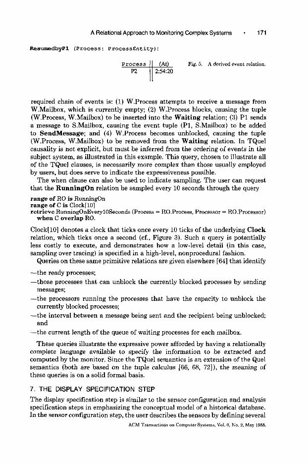
range of S is SendMessage range of W is Waiting retrieve ResumedbyPl (Process = W.Process)

valid at end of W where S.Mailbox = W.Mailbox and S.Process = Pl when S precede end of W

This query determines those processes (Process = W.Process) that were initially blocked on a mailbox (indicated by their presence in the Waiting relation), then resumed (S precede end of W) as a side effect of a message being sent by Pl (SProcess = Pl) to the mailbox (S.Mailbox = W.Mailbox). Since the valid-at clause was used, the resulting relation is an event relation (see Figure 5). The ACM Transactions on Computer Systems, Vol. 6, No. 2, May 1968.


FbsumdbyPl (Process: ProcessEntity):

Fig. 5. A derived event relation.

required chain of events is: (1) W.Process attempts to receive a message from W.Mailbox, which is currently empty; (2) W.Process blocks, causing the tuple (W.Process, W.Mailbox) to be inserted into the Waiting relation; (3) Pl sends a message to SMailbox, causing the event tuple (Pl, SMailbox) to be added to SendMessage; and (4) W.Process becomes unblocked, causing the tuple (W.Process, W.Mailbox) to be removed from the Waiting relation. In TQuel causality is not explicit, but must be inferred from the ordering of events in the subject system, as illustrated in this example. This query, chosen to illustrate all of the TQuel clauses, is necessarily more complex than those usually employed by users, but does serve to indicate the expressiveness possible.

The when clause can also be used to indicate sampling. The user can request that the RunningOn relation be sampled every 10 seconds through the query

range of RO is RunningOn range of C is Clock[ lo] retrieve RunningOnEverylOSeconds (Process = RO.Process, Processor = RO.Processor)

when C overlap RO.

Clock[lO] denotes a clock that ticks once every 10 ticks of the underlying Clock relation, which ticks once a second (cf., Figure 3). Such a query is potentially less costly to execute, and demonstrates how a low-level detail (in this case, sampling over tracing) is specified in a high-level, nonprocedural fashion.

Queries on these same primitive relations are given elsewhere [64] that identify

-the ready processes;

-those processes that can unblock the currently blocked processes by sending messages;

-the processors running the processes that have the capacity to unblock the currently blocked processes;

-the interval between a message being sent and the recipient being unblocked; and

-the current length of the queue of waiting processes for each mailbox.

These queries illustrate the expressive power afforded by having a relationally complete language available to specify the information to be extracted and computed by the monitor. Since the TQuel semantics is an extension of the Quel semantics (both are based on the tuple calculus [66, 68, 72]), the meaning of these queries is on a solid formal basis.

7. THE DISPLAY SPECIFICATION STEP

The display specification step is similar to the sensor configuration and analysis specification steps in emphasizing the conceptual model of a historical database. In the sensor configuration step, the user describes the sensors by defining several



entity and relationship relations. In the analysis specification step, the user describes the processing by defining through a relational query language several derived relations, each containing one or more entity attributes. In the display specification step, we continue to exploit the relational model [60]. Each entity relation is associated with a graphical representation. These representations have fixed aspects and aspects that depend on the values of the attributes. When the tuples of the relation are displayed, each tuple will cause an instance of the representation for the corresponding relation to be computed and displayed. For this example, we associate the Process relation with a circle. The (external equivalent of the) process identifier value will appear as text centered in the circle, and the status will be represented by the intensity of the circle (with closer to Running being darker). The value of the process identifier will also determine the vertical position of every circle (after they have been alphabetically ordered); the horizontal position of every process will be the left-hand side of the screen. The Processor relation is represented with a rectangle whose vertical position will be determined by the processor identifier value (again, in alphabetical order), which will also appear at the top right-hand corner of the rectangle; the horizontal position is again the left-hand side of the screen. Finally, the Mailbox entity relation is represented by an oval, with the value of the mailbox identifier appearing in the center and also determining the vertical position; the horizontal positions of all mailboxes are the right-hand side of the screen. The actual specifications are quite simple: 14 commands suffice for the three entity relations (as with the sensor-description language, the details of the syntax of the display specification language are not relevant, so the actual commands are omitted).

The primitive relationship relations are also associated with representations. The representations for these relations will differ from previous representations in that they will use the representations of the entities participating in the relationship. The RunningOn relation involves two entity types: process and processor. We will represent this relationship using spatial inclusion: If process Pl is running on processor A, then the iconic representation of Pl (a circle) will appear inside the iconic representation of A (a rectangle). The representation of the Waiting relation will be specified as a pointer from the mailbox icon to the process icon. Finally, the representation of the SendMessage relation is a pointer from the process icon to the mailbox icon. The actual specifications for these relationship relations consist of 11 commands.

Finally, we need a representation for time. Of the several available, we choose animationtrace, where the display changes over time as the underlying relations evolve. With animationtrace, full intensity indicates the current state with various decreases in intensity indicating past states. We augment this representation with a digital clock icon. Representations can also be associated with derived relations. In this case, we specify that the display system flash on and off the circles representing those processes that were resumed by process Pl, as stored in the ResumedbyPl relation. If we give the commands to display the Process, Processor, Mailbox, RunningOn, Waiting, and SendMessage relations, the system then displays a movie of the execution of the monitored system.

The display specification step, as just presented, has four important characteristics. First, it is closely coupled to the underlying conceptual model, the entity- ACM Transactions on Computer Systems, Vol. 6, No. 2, May 1988.


relationship model, which is also the basis for the sensor configuration and specification steps. Representations are associated with entities and with relationships. Second, there is variety in the supported representations. The currently available icons are point, line, pointer, curve, polygon, circle, text, user-defined icon, and combinations of these. The aspects that can be coupled to an attribute’s value are intensity, color, rotation, scale, transformation, horizontal position, and vertical position. Time can be represented as animation, animationtrace, four types of icons, color, intensity, blinking, or five types of geometric transla- tions. That time can be displayed in so many ways, separately or in combination, allows different aspects to be emphasized. The representation of animationtrace chosen for the example emphasizes the situation at consecutive instants of time. The alternative of representing time horizontally would emphasize the duration of particular states: The representation of states that existed for a long time would be spread across the screen, while the representation of other, short-lived states would occupy less screen space, and hence would be less noticeable. Third, the user is able to specify the representation, both of the provided relations and of those derived by the user via TQuel queries. These representations may be modified at any time, supporting the incremental development of the display specification. Finally, the commands for specifying the display are simple, allowing the user to concentrate on the task at hand: understanding the behavior of the subject system.

8. THE EXECUTION STEP

Previous sections have discussed how sensors, queries, and the display may be specified in a high-level, declarative fashion. Such simplicity and expressive power have a cost: The monitor must be able to determine which sensors to enable, what calculations to perform, and how to display the results, all with minimal guidance from the user. Fortunately, there has been much work on processing relational query languages. It is important to keep in mind, however, that there is a fundamental difference in the way that a DBMS and the monitor operate. In a DBMS, the data is present on secondary storage, and queries derive new relations, to be displayed or stored. In the monitor, the queries are made on a conceptual database; the actual data is not collected until after the query has been made by the user. Despite this difference, the techniques used in conventional DBMSs may still be profitably applied, with some alterations, to a relational monitor. This section will address enabling the sensors, generating the data, analyzing the data, and displaying the derived relations.

8.1 The Relational Algebra

Tuple calculus queries, such as those formulated in Quel or TQuel, express what derived information is desired, letting the DBMS determine how the information is to be derived. Relational algebra expressions serve the latter purpose. The DBMS converts each tuple calculus query into an algebraic expression. As this expression is often quite inefficient, optimizations are applied that convert the initial expression into a semantically equivalent one that is more efficient.

We assume that the reader is familiar with the common relational operations selection ( uF), projection ( 7rdld,. &, Cartesian product (x), and intersection (n)



[72]. Converting a Quel query into a relational algebra expression is straightforward: first take the Cartesian product of the underlying relations (each associated with a tuple variable used in the query), apply a selection with the formula from the where clause, and then apply a projection, with the attributes from the target list. The algebra may be extended to handle TQuel’s valid and when clauses, involving the extension of the projection and selection operators, respectively [46]. In the remainder of this paper, we give a somewhat simplified version of this algebra, emphasizing the correspondence with the conventional relational algebra. The projection and selection operators remain, but only involve the explicit, nontemporal domains. The valid clause is handled by a temporal variant of the projection operator, denoted by 7rr. This operator will “project out” those intervals designated by expressions in the valid clause. The when clause is handled by a temporal variant of the selection operator, denoted by gT. The subscript for this operator consists of the temporal predicate specified in the when clause. The operator will “select out” those tuples satisfying the predicate. The aT and aT operators are employed in the same manner as the r and c operators. For example, the query for ResumedbyPl has the corresponding temporal relational algebra expression

~W.Process ~LhlofW dprecedeendofW ( (

(: =: (. US Madbox W Madbox CS Process=Pl (Waiting, x SendMessages))))) (E1)

and the query for RunningOnEverylOSeconds has the corresponding expression

d&&erlapRO (RunningOnRo x Clock[lO]c)) UW

Note that the tuple variable associated with a relation is indicated as a subscript on that relation.

A more substantial modification is to make the operators incremental, so that they operate on streams of tuples, one at a time, possibly generating one or more output tuples whenever an input tuple arrives [45]. The selection and projection operators (both conventional and temporal) are straightforward to extend to operating on streams rather than sets. Each such operator would generate at most one output tuple for each input tuple, and no tuples would have to be stored, assuming that the projection operator does not perform duplicate elimination. The Cartesian operator is more complex, for two reasons: it is a binary operator and it requires internal storage. It stores the tuples arriving from the left, and concatenates all of these tuples to tuples arriving from the right, thereby generating multiple output tuples for each input tuple. The brute-force Cartesian operator requires storage for all the input tuples; more space-efficient variants also exist.

In summary, each TQuel query is converted into an algebraic expression consisting of the underlying relations and the incremental temporal operators 7r, 7rT, u, UT, and X. Once these expressions for the TQuel queries have been generated, they can be used to enable sensors and analyze the incoming data.

8.2 Incorporating Primitive Relations in the Algebra

Enabling sensors manually in a complex system is very difficult for the user, due to the potentially large number of sensors. One alternative, the brute-force



enabling of all sensors, is excessively inefficient. Hence, the monitor should handle the task of determining which sensors to enable, and should enable only the necessary sensors, thereby filtering out unnecessary data packets. Filtering should occur early and often, so that scarce communication and processing resources are not expended on data that are later discarded.

The monitor must extract as much information as possible from the query to enable the correct sensors. This information is used to enable the appropriate traced sensors and to trigger the appropriate sampled sensors at the appropriate times on the appropriate entities. The strategy employed here modifies the temporal relational algebra to accommodate primitive relations. In queries involving derived relations, the expression associated with the derived relations is substituted into the expression for the current query. In the following subsections, we first introduce a new operator to take the place of primitive relations. This operator enables a particular sensor as a side effect. The algorithm given above, which translates TQuel statements to algebraic expressions, is extended to specify defaults for which sensors to enable. Transformations then map these expressions into semantically equivalent expressions that enable fewer sensors. These transformations are similar to those used to optimize conventional algebraic expressions generated from static query languages.

These steps are applied to Expressions (El) and (E2), mapping them first into expressions that enable sensors fairly freely. Optimizations are then applied, resulting in expressions that are careful to enable a minimal number of sensors.

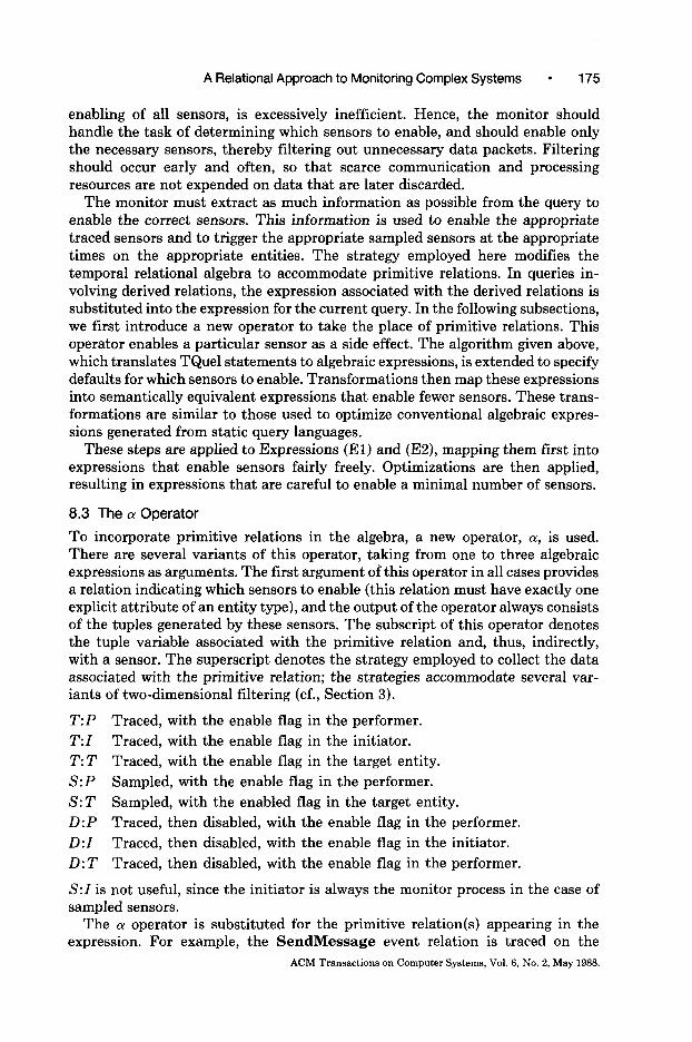
8.3 The CY Operator

To incorporate primitive relations in the algebra, a new operator, CY, is used. There are several variants of this operator, taking from one to three algebraic expressions as arguments. The first argument of this operator in all cases provides a relation indicating which sensors to enable (this relation must have exactly one explicit attribute of an entity type), and the output of the operator always consists of the tuples generated by these sensors. The subscript of this operator denotes the tuple variable associated with the primitive relation and, thus, indirectly, with a sensor. The superscript denotes the strategy employed to collect the data associated with the primitive relation; the strategies accommodate several variants of two-dimensional filtering (cf., Section 3).

T:P Traced, with the enable flag in the performer.

T:I Traced, with the enable flag in the initiator.

T:T Traced, with the enable flag in the target entity.

S:P Sampled, with the enable flag in the performer.

S:T Sampled, with the enabled flag in the target entity.

D:P Traced, then disabled, with the enable flag in the performer.

D:I Traced, then disabled, with the enable flag in the initiator.

D:T Traced, then disabled, with the enable flag in the performer.

S:I is not useful, since the initiator is always the monitor process in the case of sampled sensors.

The (Y operator is substituted for the primitive relation(s) appearing in the expression. For example, the SendMessage event relation is traced on the



initiator. If this relation was referenced in a query through the tuple variable S, it would appear in the algebraic expression as

asT”(?).

The “I” is replaced with an algebraic expression computing the processes for which this sensor is to be enabled. Let us suppose that this expression was simply the constant process entity identifier Pl. Then this operator would cause the enable flag for the SendMessage sensor to be set in the process named by Pl. When the process named by Pl executed a SendMessage operation, the sensor would fire and would generate a data packet containing the entity identifier for the process (i.e., Pl), the entity identifier for the mailbox being sent to, and a time stamp (cf., Figure 4). This data packet would be converted into a tuple, which would be contained in the relation output by the a operator. Like the other operators, the (Y operator is incremental, both in the tuples it accepts from its argument(s) and in the tuples it generates. In this example, each time the SendMessage sensor generates a data packet, the a operator subsequently emits a tuple. For some primitive relations, the LY operator converts the data packets indicating event occurrences into interval tuples, as discussed in Section 4.

The &T:P, &T:Z, &T:T, &D:P, &D:Z, and aD:T operators have one argument, the relation comprised of entities containing the flag to be enabled. The czD operators, termed disable traced, are associated with sensors that immediately disable their enable flag after generating a data packet. The cyszp operator has two arguments: the entity containing the enable flag (the performer), and a specification of when to sample. The explicit attributes of tuples of the second argument are ignored; each entering tuple triggers a request by the monitor to enable the appropriate sensor, causing sampling to occur. Generally the second argument is the Clock relation. The aStT operator has three arguments: what to enable (the target entity), when to sample, and who to request the sampling of (i.e., the performer of the sampling). The third relation must have one explicit attribute, of an entity type. In all cases, the output consists of the tuples in the relevant primitive relation generated as a side effect of tuples entering the a operator.

A few examples will clarify the differences between the types of (Y operators. We have already examined the SendMessage event relation. The RunningOn interval relation is sampled on the-performer, and would appear in the algebraic expression of a query referencing it through the tuple variable RO as

c&f(~ “) ., .

The first “?” would be replaced with an expression computing processes; the second “?” would be replaced with an expression computing events, at which times the request to sample would be conveyed to the processes comprising the first argument. The Waiting interval relation is disable traced on the target mailbox:

When entities arrive from the expression replacing the “T”, the Waiting sensor is enabled. However, it is immediately disabled (by the sensor) once the operation occurs and the sensor generates the data packet.



The CY operator is distinct from the other relational operators in that the output tuples are not simply a function of the input tuples. Instead, the output tuples comprise a subset of the primitive relation associated with the operator, the subset being determined indirectly by the input tuples. Hence, the tuples output by olg’(P1) will be a subset of the tuples conceptually present in the SendMessage primitive relations: exactly those tuples with an initiator of Pl. Equivalently, the output tuples comprise the data packets generated by the associated sensor (e.g., the SendMessage sensor), which was enabled as a side effect of input tuples entering the CY operator. The incremental execution of a temporal relational algebraic expression is coupled with the sensors in the subject system through the LY operator(s) appearing in the expression.

There is one additional connection between the input and output tuples of an (Y operator. As an example, we will use cyst” again. The set of entity identifiers present in the input tuples of this operator (in the case, only Pl) will be a superset of the set of entity identifiers present in the Initiator position of the output tuples, since only those entities were ever enabled. Similar statements can be made of each variant of (Y operator. The (Y operator is similar in this aspect to Horwitz’s selective retrieval function, which generates tuples having particular values for particular attributes [28].

8.4 Entity Sources

The algorithm translating TQuel queries to algebraic expressions must specify defaults for which sensors to enable, that is, the arguments to the CY operators. Here the entity relations (defined in Section 3) for the entity types in the subject system are used. These relations generate tuples naming all existing entities of that type and are termed entity sources. Entity sources are denoted by the entity name: Process denotes the entity relation and hence the associated sensor that generates all existing process entities (recall from Section 3 that this sensor may be found in the process manager).

Entity sources complete the terms replacing the primitive relations. The term replacing SendMessage in (El) is

&‘(T, rOceSS (Process))

Note that a projection operator is necessary for those entity relations that contain more than one attribute. For the second argument of sampled a! operators, which specifies when to sample, one of the primitive clock relations is used as a default. The term for RunningOnRo appearing in (E2) is

&‘(Processor, Clock)

(note that Clock is used as an entity source), and the term replacing Waitingw in (E2) is simply

&T(Mailbox)

The specific (Y operator substituted for each primitive relation appearing in the query can be determined solely from the sensor specification of that relation (cf., Section 3). The default arguments are also easily determined from information in the sensor specification.



The final algebraic expression for the ResumedbyPl query can now be presented (compare with (El)):

*W.Process ~aTtendofW ‘&recedeendofW ~S.Mailbox=W.Mailbox ( ( (

(~s.Process=P1 (&T(Mailbox) x as’:‘(~P,,,,,,(Process))))))) (E3)

as can the expression for RunningOnEverylOSecond query (compare with 032)):

rift ,(a: overla,, Ro(ag:(Processor, Clock) x Clock[lOlc)) (E4)

Entity sources are associated with sensors that are permanently enabled. Note that an entity relation need not be an entity source if it never appears as a default parameter of an (Y operator, but an entity source must be an entity relation (or the Clock relation).

8.5 Data Generation and Analysis

At this point, the TQuel query, which is declarative in nature, has been mapped into an algebraic expression containing the 7r, ?yT, u, aT, X, and a! operators, as well as entity sources. Recall that the temporal relational operators are incremental, in that they take streams of input tuples one at a time and possibly generate one or more output tuples whenever an input tuple arrives. The entity sources are also incremental, generating tuples whenever a new entity is created (a tuple is also generated when an entity is destroyed). The expression is started by having the constants and entity sources (e.g., Mailbox and Process in Expression (E3)) generate initial tuple streams. These streams are comprised of unary tuples, each containing one entity identifier. Expression (E3) is primed with two streams, one containing a tuple for each process and one containing a tuple for each mailbox, acquired from the process communication manager. Similarly, Expression (E4) is primed with three streams: two generated by the clock and one containing a tuple for each processor, acquired from system configuration tables.

The initial tuples flow into the specified operators. In the case of (Y operators, the tuples indicate which entities contain the appropriate enable flags to set. The monitor deduces the entity’s location from the entity identifier (the mechanism presented in Section 2 assumed that this was possible) within the tuple, and sets the enable flag in the entity, thereby enabling the sensor. Once enabled, the sensors generate data packets, which are gathered and sent to the monitor, where they are separated by sensor identifier. The sensor identifier names a particular a! operator (or operators) associated with a tuple variable ranging over the primitive relation associated with a sensor. The data packets containing the correct sensor identifier form the tuples output by the CY operator. Hence, tuples flowing into the cy operator indirectly enable various sensors, which generate data packets that eventually comprise the output of the a! operator. The tuples flowing into a! operators representing intervals specify both when to enable a sensor on a particular entity and when to disable that sensor on that entity. The interpre- tation of the expression continues until all the sensors are disabled in the course of execution. ACM Transactions on Computer Systems, Vol. 6, No. 2, May 1988.


The tuples flowing out of the cy operators flow into

-the r operator, which outputs a tuple each time a tuple flows into it, with fewer attributes;

-the rT operator, which outputs a tuple each time a tuple flows into it, while calculating the time stamp for the output tuple as a function of the time stamp(s) in the input tuple;

-the u operator, which outputs the tuple if it satisfies the given predicate on the explicit attributes;

-the aT operator, which outputs the tuple if it satisfies the given predicate on the implicit time attributes; or

-the x operator, which concatenates tuples flowing in on the left side with tuples flowing in on the right side.

Each expression is a data-flow program [l] in the form of a tree, with entity sources at the leaves and operators at the interior nodes. Tuples flowing out of the root of the tree are displayed to the user or stored for later analysis. Tuples flowing across interior branches exist for only a short amount of time. In particular, intermediate relations, which consist of all tuples flowing over a given branch of the tree, are never fully constituted; at any time, small portions of these relations may be found flowing across a branch or residing in the local storage of an operator.

For each TQuel query, there are potentially many algebraic expressions that are semantically equivalent to the query, yet may vary greatly in efficiency. The steps detailed in Sections 8.1-8.4 result in one of these algebraic expressions. Unfortunately, this expression is usually quite inefficient. Expression (E3) is an example. The Mailbox sensor generates all the mailboxes, and the Process sensor generates all the current processes. The Waiting sensor is enabled for the mailboxes, and the SendMessage sensor is enabled for the processes. As processes send messages, data packets are produced by the SendMessage and Waiting sensors. The Cartesian product generates a tuple for each combination of tuples generated by the LX operators associated with the Waiting and SendMessage sensors; the number of generated tuples grows as the product of the total number of block and send operations by all processes. Almost all the tuples are subsequently discarded by the three selection operators. Finally, one explicit and one implicit attribute are projected out, forming the resulting tuples. As another example, the processing of Expression (E4) results in samples that are taken every second, then concatenated with a tuple for every clock tick, and then discarded if the time the sample was taken does not correspond to the time a particular clock tick occurred. The (in)efficiency of Expressions (E3) and (E4) is a direct result both of the expressive power of the nonprocedural query language TQuel and of the simplicity of the initial translation into a relational algebraic expression. Clearly, this inefficiency is unacceptable and must be ameliorated if the relational approach is to be a viable one.

8.6 Algebraic Optimization Transformations

The term “optimization” is a misnomer; a more accurate term is “improvement,” for an optimal solution almost never results. However, we will continue to use this term, with the understood proviso.



One benefit of using the relational model with monitoring is that traditional optimization techniques may be utilized directly. One example is the transformation

dR1 x Rz) + R1 x dRz) (01)

which applies if the predicate F only involves attributes from Rz. This transformation can dramatically reduce the number of tuples generated by the Cartesian product, since uninteresting tuples are discarded before rather than after the Cartesian product. This optimization can be applied once to the Expression (E3), with the substitutions

S.Process=Pl for F. Waiting for RI. SendMessage for &.

resulting in

TW.Proces~ ~~endofW ( ( ~~~~reeedeendofW ( ~S.mailbox=W.mailbox

GT(Mailbox) X ~s.P~~~~~~=P~(~~‘(~P~~~~~(P~oc~ss))))))) UN

Note how the selection us.Process=P1 was moved to before the Cartesian product operator. A collection of such transformations has been developed for the conventional relational algebra [62]; these transformations apply directly to the temporal relational algebra [46].

A second class of transformations involves the (Y operator. Using entity sources as arguments to (Y corresponds to enabling everything. However, transformations may be applied to map expressions into semantically equivalent expressions by replacing entity sources with more constrained expressions that (a) enable fewer sensors, (b) replace sampling with tracing, or (c) sample less frequently. Approx- imately 10 transformations, each with several variants, have been developed thus far; only a few will be discussed here. The first shares some features with the one just given:

Ut.initiator=K((YtT:I(E)) + aT:‘(Ul=K(E)) (02)

In these transformation schemas, variables to be substituted are in italics. Intuitively, this transformation states that, rather than enabling a sensor on a large number of processes (a(E)) and then discarding (a) many of the data packets so generated, you should enable the sensor on only the relevant processes. The reason that a~‘(~~=&)) appears on the right-hand side rather than simply the constant K is that a:’ should be enabled for process K only if E contains K. Otherwise, no sensors should be enabled.

In this transformation, E is an arbitrary algebraic expression that returns a relation with one attribute of type process; t is a tuple variable associated with a primitive relation traced on an initiator; K is a constant denoting a particular process identifier; and “1” is the name of the first attribute. In the expression before the transformation is applied, the appropriate sensor is enabled for all processes, with most of the resulting data packets (tuples) discarded by the selection operator. In the expression resulting from the transformation, if E contains the process K, then the appropriate sensor in that process is enabled. ACM Transactions on Computer Systems, Vol. 6, No. 2, May 1988.


There is no need to discard any data packets, because all the data packets are guaranteed to have a performer of K. This transformation can be applied to Expression (E5), with the substitutions

S for t.

S.Process for t.initiator.

Pl for K. ~p,,,ess (Process) for E.

resulting in

~W.Process TatendofW OSprecedeendofW tT tT ( ~S.Mailbox=W.Mailbox

(c#‘(Mailbox) x ct~‘(a,=P1(ap,,,,,,(Process))))))) 036)

There is another transformation that is even closer (semantically, not syntac- tically) to the traditional one that moves a selection to before a Cartesian product:

&precedeendoft ~E2.A=t.target ( bfzT(&) x Ed + afrTU% n ~E,.A 0%)) (03)

In the left-hand side of this transformation, the attribute A, which must be in EP, is being used to select tuples generated by a:“. An example may be found in Expression (E6), where S.Mailbox is used to select tuples generated by c&r. In the left-hand side of the optimization, (Y~ generates a stream of tuples, which are concatenated with tuples in Ez, and then most are thrown away, based on a comparison of the target with -an attribute of Ez. However, since the associated sensor is disable traced on the appropriate attribute (the target) anyway, the filtering may occur when enabling the sensor, rather than later, after the unnecessary data packet has been generated. On the right-hand side of the transformation, 0~:‘~ is enabled on only the relevant entities, as indicated by the attribute of Ez (the entity must also be in El, or it would not have been enabled by the original expression). The temporal selector aT on the left-hand side is necessary because Es cannot be used to enable o$’ if t finishes before E,.

There are three restrictions on the application of this transformation:

(1) Only attributes associated with the tuple variable t may be used by operators on the tuples produced by the expression; those found in E2 are not available for further use.

(2) The attribute begin of t is not needed, because (Y~ may not have been enabled when begin of t occurred, even if it was enabled when end of t occurred.

(3) E, is an expression computing an event relation.

This transformation may be used on Expression (E5), using the substitutions

W for t.

W.Mailbox for t.target.

Mailbox for El. asT:l(ul,pl (Pp roce9s (Process) ) ) for EZ .

S.Mailbox for E2.A. “S precede end of W” for “E2 precede end of t”.



resulting in

~W.Process ~Lmio*w ( WT(Mailbox fl ~S,Mailbox(~~‘(fll=~1 (ap,,,,,(Process))))))) (E7)

There are many variants on this transformation, each on a different kind of (Y operator and each having different constraints. Note that, while entity sources are still at the leaves of the parse tree, the cy operators are no longer just above them, as was the case in all the previous expressions. This example shows that (Y operators can appear anywhere within the tree, thereby utilizing the full power of the relational algebra in determining which sensors to enable.

It should be noted that complications arise when multiple (Y operators referring to the same primitive relation are present in a collection of queries. Either this situation must not be allowed, or the monitor must be able to sort out the incoming data packets from the sensors and determine which LY operators to send each packet to, or the (Y operators must perform this selection themselves. The correct filtering is still performed at the sensors, in any case.

A third class of transformations involves entity sources. We give two here:

alaA?)+ K (04)

?flE*E (0%

Both derive from the definition of the entity source ? and elementary set theory, and assume that K and E are of the same entity type as ?. The first states that selecting a particular entity out of an entity set results in that entity (if the entity can be named, it must be in the entity set). The second states that taking the intersection of a subset of entities and an entity set results in that subset. The first transformation can be applied to Expression (E7), substituting “Pl” for “K" and “~Process(Process)” for “?” to get

~W.Process (r LndofW aw ( D’T(Mailbox fl ~S,~,i~b~x((Y~‘(Pl))))) 033)

The second transformation can be applied to this expression substituting “as.Mailbox((YST:‘(Pl))” for "E" and “Mailbox” for “?” to get

~W.Process ~LndofW ffw ( ( D’T(pS.Mailbox((Y~‘(P1))))) (E9)

The fourth class of transformations involves the Clock event relation. This relation can be used to specify sampling rates; several of the transformations allow the monitor to handle this. The transformation

*at CbCToverlapt (afTP(E1, E,) x Clock[i]c)) + afzP(R, Ez r-T Clock[i]c) (06)

modifies the second argument of the (Y operator, which specifies the sampling frequency. The subscript C on Clock[i] indicates the tuple variable associated with this predefined relation. Recall that the postfix “[i]” denotes a clock that ticks once every i ticks of the underlying clock. The right-hand side specifies that the sensor is to be sampled less often.

A second transformation

Clock[n] n Clock[n*i] -+ Clock[n*i] (07) ACM Transactions on Computer Systems, Vol. 6, No. 2, May 1988.


allows longer frequencies to be used (note the similarity with optimization (05)). Both transformations may be applied to Expression (E4). The first transformation results in

&(Processor, Clock rl Clock[lO]c)

and the second in

a%(Processor, Clock[lO]c) WO)

(Clock is shorthand for Clock[l]) with the result that the RunningOn sensor is sampled every 10 seconds, rather than the default sampling frequency.

A final class of transformations selects a more efficient variant of an operator based on the temporal ordering of the input tuples to the operator and the desired temporal ordering of the output. For example, the Cartesian product operator in its most general form must store internally all incoming tuples from the left, so that they can be later concatenated with incoming tuples from the right. If the tuples on both sides were in temporal order, and their overlap was desired, a much more efficient Cartesian product may be used:

where x1 denotes the particular variant of the Cartesian product. This operator would only store those tuples from the left that could possibly overlap with those from the right, discarding the rest from internal storage.

The transformations from the five classes (traditional, involving the (Y operator, involving entity sources, involving the Clock event relation, and involving more efficient variants of an operator) are repeatedly applied in order to the algebraic expression until no more are applicable (the application of one transformation can enable the application of another transformation). A comparison of the processing resulting from the “before” Expression (E3) with the processing resulting from the “after” Expression (E9) for the ResumedbyPl query indicates the increase in efficiency that is possible. The previous examination of Expression (E3) revealed that it was very inefficient. The transformed expression, on the other hand, is quite efficient. First, the Send sensor is enabled only for the Pl process (LYEI(P When Pl actually sends a message, the mailbox identifier is extracted from the data packet (rs.Mailbox), and the Waiting sensor is enabled for this mailbox ((rsT). Since the enable flag is actually an integer (cf., Section 4), multiple send operations by Pl are handled correctly. When a process is unblocked, receiving the message, the Waiting sensor sends a data packet containing the process identifier and the mailbox identifier. This sensor is also disabled by the monitor, awaiting reenabling when Pl sends another message to the mailbox. The process identifier and end time are projected out of the data packet, forming the resulting tuple. Using the sample data from Section 4, Expression (E9) is primed with the single process identifier for Pl; tuples flow out of (YC’ operators (those shown in Figure 2) and into the projection operator, resulting in the tuples (M3, 2:00:05), (M4, 2:00:06), and (M7, 2:51:13). These tuples successively flow into &r, which subsequently generates the tuple (P2, M7, 2:45:29, 2:54:20), which flows into the two projection operators, resulting in



the tuple (P2, 2:54:20) as shown in Figure 5. The number of generated tuples is linear in the number of send operations by Pl.

Expression (ElO) is also much more efficient than the initial attempt (Expres- sion (E4)). The optimized expression specifies that the RunningOn sensor is to be sampled by the scheduler of each processor every 10 clock ticks.

The relative increase in efficiency observed in these two examples is primarily an indication of the gross inefficiency of the unoptimized expression; the absolute efficiency suggests that the optimizations enable the minimal sensors and perform just the computations needed to derive the desired information.

8.7 Display Generation

Once the tuples in the derived relation have been computed by the optimized algebraic expression, they are used to generate the images on the display device. For each tuple, a graphical object (a data structure) is first constructed from the fixed aspects of the representation associated with the derived relation (the possible graphical aspects were reviewed in Section 7). The attribute-dependent aspects are then calculated, based on the values present in the tuple. Temporal modifications dictated by the specified time representations are then made to the graphical object, which is then translated into appropriate calls to the low- level graphic routines to display the object. Incremental display modification over time is possible because the fixed aspects of the graphical representation are differentiated from the attribute-dependent aspects, which are further differentiated from the temporally dependent aspects. Details of the display processing are given elsewhere [60].

9. IMPLEMENTATION

While the analysis in Section 2 demonstrated the many advantages of the relational approach over traditional monitoring techniques, two substantial issues remain: system complexity and performance. The relational approach requires a sophisticated monitor: Can the functions of the monitor be partitioned so that each component is of manageable size and the interaction between components is well defined? Regarding performance, several concerns arise. Can the data- collection mechanism be implemented so that it is extremely efficient when disabled and relatively efficient when enabled? Is distributed data collection on a large multiprocessor feasible? How effective are the algebraic optimizations in practice, both relatively, in terms of increased performance, and absolutely, in terms of data packets per second processed? Can an evolving display specified declaratively be generated in real time ? To address these questions, we have completed one prototype implementation and have made significant progress toward a second implementation. These implementations have been instrumented, and the bottlenecks identified.

The system monitored by the prototype was Cm*, a tightly coupled multiprocessor composed of 50 DEC LSI-11s (each a 0.3 MIP machine) and a substantial amount of memory [17, 20, 691. Two operating systems were available on Cm*: StarOS [19, 32, 331 and Medusa [53]. The Berkeley UNIX 4.2BSD operating system, running on either DEC Vaxes or Sun workstations, is the subject system of the second implementation. While Cm* and its operating systems are highly



decentralized and oriented toward research, the UNIX operating system is centralized and oriented toward providing a flexible program development environment. These differences are reflected in some aspects of their monitors. The two implementations were developed over several years at two institutions, Carnegie-Mellon University and the University of North Carolina; various col- lections of the modules have been integrated at different times.

The monitor consists of two main components: a remote monitor, performing those functions requiring close interaction with the user, and a resident monitor, performing the functions requiring close interaction with the subject system. This separation is necessary when monitoring a distributed system, where a resident monitor exists at each processor, sending collected data to the centralized remote monitor, which may or may not execute on one of the processors being monitored. Functionally, the resident monitor collects the data packets and interacts with the operating system, and the remote monitor analyzes and displays the monitoring data.

In both the prototype and the second implementation, the remote monitor ran on a Vax under UNIX and was itself composed of four modules. The TQuel compiler translated the query into an initial algebraic expression. The parse tree for this expression was termed an update network, referring to the tuples flowing across the arcs. The movement of tuples through this network was handled by the update network interpreter. The remote accountant handled the Ethernet protocol, sending tuples to the interpreter and sending commands to the resident monitor. The remote accountant is merged with the resident accountant in the second implementation, since both execute on the same machine. The display system mapped the derived tuples into graphical images on a Sun workstation.

Three resident monitors were implemented, one on StarOS [63], one on Medusa [25], and one on UNIX [16]. The remote monitor on the Vax communicated with the resident monitor on Cm* over an Ethernet [47], a high bandwidth network.

The implementation carried all aspects sufficiently far to demonstrate feasibility and to investigate efficiency aspects. More specifically, the sensor installation component, the update network interpreter, the three resident monitors (the remote accountant, the TQuel parser and code generator, and the display system) are essentially complete. The TQuel semantic analysis phase was only partially implemented, and the optimization phase was designed but not implemented. The prototype showed that it is possible to partition the monitor into manageable components, interacting through well-defined interfaces. While much work would be required to make the monitor fully general and robust, the implementation was sufficiently complete to indicate that there were no insur- mountable problems in the way of a fully functional system.

Several of the components were instrumented to determine the overall performance of the monitor. The rest of this section will briefly discuss the performance of the sensors, the Ethernet protocol, the update network interpreter, and the display system. Details are given elsewhere [60, 631.

The efficiency of the data-collection mechanism is important, for it determines the monitoring granularity, that is, the level of abstraction at which the monitoring takes place. We will first examine the Cm* data-collection mechanisms, as they have been studied more thoroughly; the UNIX mechanism demonstrates the generality of the model and will be discussed shortly.



The Cm* data-collection mechanisms supported strong type checking, multiple type managers, and a high degree of filtering. Because both StarOS and Medusa are object-oriented operating systems, there was a natural fit between the data- collection model of typed entities and type managers. Space was allocated in each object to be monitored for a reference to an object containing the enable bits and a buffer for the data packets. The data packets were removed asynchronously from these buffers by the resident monitor. Allocating additional space for a 32-bit reference was much easier than allocating space directly in each object for the buffer and allows the buffers to be shared among many objects.

Several StarOS sensors were repeatedly invoked to determine their execution efficiency. Two versions of these sensors were studied. Inline code tested whether the event was enabled, and, if so, called a procedure to construct and store the data packet. The second version consisted totally of inline code. Both versions were implemented using existing microcoded operations for efficiency. As ex- pected, the code in the first version was smaller, requiring from 29 to 44 words, as compared with 41 to 96 words for the second version. However, since the procedure is itself 350 words long, inline expansion requires less space than procedure calls if there are less than about 20 sensors in the process. If no sensors were enabled for a process, the sensors (in both versions) took only 15 microseconds, equivalent to 2 store instructions on an LSI-11, representing the cost of installing sensors in a process and then never using them. If the transformations discussed in Section 8.6 are effective, only a small number of sensors will be enabled; most processes will have all their sensors disabled. If some sensors were enabled in the process, an additional check was required, and a disabled sensor took 165 microseconds, equivalent to 23 store operations. A microcoded version of the sensor would take approximately 90 microseconds in an equivalent situation. An enabled inline sensor requires 600-1400 microseconds per invocation, depending on the amount of data stored in the data packet. This execution time is equivalent to 85-200 store instructions, or 6-14 procedure calls. Permanently enabled sensors are faster by about 150 microseconds. The procedure-call version, when enabled, requires 1850-2330 microseconds, 60-300 percent slower than the inline version. The reason the inline version is superior in both space and time is that the code for each sensor is generated automatically in the sensor installation step, and therefore can be customized to the specification of the sensor. Hence, the monitoring granularity for this implementation of sensors is larger than a procedure call, but perhaps equal to a procedure that does something interesting, in turn calling other procedures. Given this sensor efficiency, with intelligent filtering reducing the monitoring overhead to 1 percent, the 50 processors would generate approximately 500 data packets per second.

The UNIX sensors store the data packets in a single kernel-resident buffer, via a new system call if the sensor is in a user process, or directly if the sensor is in the kernel [ 161. The resident monitor is a user process that invokes a second option of the monitor system call to extract the data packets from the buffer and send them on to the remote monitor. The resident monitor is also responsible for enabling and disabling sensors in both the kernel and in user processes, through yet another option of the system call. ACM Transactions on Computer Systems, Vol. 6, No. 2, May 1968.


UNIX is not object oriented; the only identifiable object supported by UNIX is the file. However, the data-collection model can be applied to UNIX in an abstract fashion. There are several entity types, each corresponding to a data structure in the kernel: file (represented by an inode on disk or in memory), pipe (an entry in the pipe table), socket, device, etc. Each of these data structures must be expanded to include the enable flags. The flags can only be modified by the kernel, via a request from the resident monitor. The type manager, which is the performer for operations on entities of these types, is the kernel, arbitrarily assigned the process id 0. The entity identifier for the object is usually an index into the appropriate table (file identifiers and process identifiers are exceptions- they are stored within the table entry). At this point, only the file system of the kernel has been instrumented; adding new sensors is primarily a task of understanding the code well enough to place the sensors correctly.

Invoking the monitor system call for each data packet is necessary because the value of the clock is maintained in kernel space; lower performance is one result. The round-trip time for a system call varies across versions of UNIX and the hardware, but is currently at least 250 store instructions. Since the UNIX system is a single processor system (we have not yet extended data collection to function across several networked UNIX machines), the data packet generation rate is much lower than for Cm*: approximately 40 data packets per second, again assuming a monitoring overhead of 1 percent.

A second concern is the feasibility of distributed data collection on a large multiprocessor such as Cm*. Data collection is divided between the sensor storing the data packet in a shared buffer, the resident monitor extracting the data packets from the buffer and assembling them into larger packets to be sent to the Vax, and the remote monitor receiving data from Cm* and passing it onto the update network interpreter. The sensor, resident accountant, and remote accountant all execute asynchronously on separate processors. Apart from the performance of the sensor, which was discussed above, the maximum sustainable transmission rate between the resident and remote monitors is another potential bottleneck in data collection.

The Ethernet protocol is a variant of the Ethernet File Transfer Protocol (EFTP) [61], simulating a transmission from the resident monitor (the host) to the remote monitor (the slave). The protocol uses checksums, time-outs, and packet retransmission for reliability. Commands, such as “enable this sensor,” are incorporated into the protocol in acknowledgment packets [26]. Using the actual record and packet sizes and observing the transmission rate for the standard EFTP, a maximum transmission rate of 600 event records per second was calculated. This rate is adequate to handle the data being generated by the sensors.

The execution of an optimized algebraic expression, generated from a declarative, calculus-based TQuel query, is yet another potential bottleneck. The efficacy of the optimizations and the performance of the update network interpreter were measured using a small set of relatively complex TQuel queries. The initial update network, before optimizations were performed, could process approximately 3 input tuples per second (assuming a dedicated Vax 11/760). Two stages of optimization were performed manually to assess their effect. The first



stage applied transformations from two of the five discussed in Section 8.6: traditional algebraic transformations and transformations that substitute a more efficient variant of an operation in the expression. To simulate the effect of the other optimizations, we manually enabled only the relevant sensors. The interpreter was unchanged in the first stage. This stage resulted in a speedup of 5, to 15 input tuples per second. The second stage involved substituting the interpreter and general operator algorithms with a LISP function. Conceptually, the entire algebraic expression was converted into a specialized operator. The LISP function was then compiled by the FranzLISP compiler into Vax assembly language. The resulting code could process approximately 600 input tuples per second, resulting in an improvement of more than two orders of magnitude. This rate is adequate to accommodate the tuples generated by Cm*. In the second implementation, we are reimplementing the TQuel compiler, optimizer, and update network interpreter, and hope to obtain even higher tuple throughput. Initial indications are promising; the processing time per tuple has dropped by another factor of two.

The final concern is that of display generation. As with the other components, the display system prototype emphasized ease of implementation over efficiency. In particular, the current system does not exploit the distinction between fixed, attribute-dependent, and time-dependent aspects; the entire graphical display is recomputed with each change. Nevertheless, measurements of the prototype indicate that it can accept between 17 and 25 tuples per second, for a fairly complex display (i.e., several times more complicated than that discussed in Section 7). This rate is in terms of derived tuples, which will usually be fewer in number than input tuples. On the other hand, the algebraic optimizations attempt to enable only the relevant sensors, so the ratio of output to input tuples is kept fairly high. This ratio is highly dependent on the queries specified by the user; we did not have an adequate collection of representative queries to arrive at a good estimate. If we are conservative and assume an equal number of input and output, then the display system is a factor of 20 too slow when used with Cm*; the performance is already in the ballpark when used with a single-processor UNIX system, due to the greatly reduced tuple generation rate. We have identified many potential optimizations, and feel that a speedup of 20 is relatively straightforward. One other consideration is the speed at which the human visual system can process an evolving screen-perhaps that limitation will be reached first.

The general result of these measurements is that, given the monitoring granularity supported by this implementation, the monitor can indeed contend with the number of event records generated by the 50 processors in Cm*, with the exception of the current display system. Hence, it is possible to implement a monitor supporting the high-level conceptual viewpoint of a dynamic relational database on the system’s behavior, which can be specified using a nonprocedural temporal query language, with sufficient efficiency to monitor a large, complex, distributed system.

10. CONCLUSION

This paper has argued that the relational model provides an effective formalization of the information collected by a monitor. The relational approach presented ACM Transactions on Computer Systems, Vol. 6, No. 2, May 1966.


in this paper consists of the following five steps:

Step 1: Sensor Configuration Sensors are specified in a sensor-description language as a collection of primitive event and interval relations. The user also specifies the way in which each sensor may be enabled, as well as the location of these sensors within the code of the subject system. Sensors and their enable flags are associated with entities based on a simple model of the environment. For many sensors, the enable flag is in the initiator or the target, decoupled from the performer in which the sensor itself resides. This declarative description forms the conceptual view that the dynamic behavior of the subject system is available as the collection of historical relations. The translator for this language automatically handles the details of generating the code for each sensor and communicating needed information to the monitor, thereby greatly reducing the chance for error.

Step 2: Sensor Installation The code for the sensors is generated by the monitor. This step is entirely automatic, resulting in a fully instrumented subject system. Because sensors are generated by the monitor, there is the opportunity for automatically compensating for the monitoring artifact.

Step 3: Analysis Specification TQuel queries are made on this fictional database. This language provides a powerful user interface for querying the monitor concerning the behavior of the system.

Step 4: Display Specification At the same time, the user specifies the graphical representation of the derived relations. In the relational approach, displays are specified in a declarative fashion by associating graphical aspects with entities and relationships, for both primitive and derived relations. The iconic representation of entities and multiple time representations allow the user to visualize the derived relations in different ways.

Step 5: Execution The queries are first converted into relational algebra expressions, which, are optimized through the application of a series of conventional and monitoring- specific transformations. Processing is started by enabling sensors associated with the primitive relations appearing in the expression. Our approach makes use of the CY operator and a collection of optimizations to determine precisely which sensors to enable. The monitor uses information from the sensor specification and the algebraic expression to automatically enable only relevant sensors. The entity identifier is used to locate the entities that contain the enable flags. Special techniques allow temporal ordering of data packets from multiple buffers. As tuples flow through the expressions, other sensors are enabled, thereby creating other tuple streams. The tuples flowing out of the expressions are displayed as directed by the user.

The majority of work in monitoring has concerned the development and application of techniques within the context of the traditional approach [50, 511. In the remainder of this section, we examine other research that also addresses inadequacies of the traditional approach.



The basic idea behind the approach espoused here, using historical databases to formalize dynamic information, has been suggested in various guises by others [15, 18,38-40, 561. Relational databases have also recently been applied to other data managed by a programming environment [29, 30, 40, 411. High-level languages for specifying the analysis to be performed by the monitor have also been proposed. Linton suggested using Quel, Garcia-Molina et al. suggested using Sequel, LeDoux and Parker used Prolog, and DiMaio, Ceri, and Reghizzi used Ada. Quel, Sequel, and Ada, because they have no natural way of expressing time-dependent queries, are inappropriate for this application. Prolog can be used to express time-dependent queries. Interval logic [23], regular expressions augmented with a shuffle operator [5], and path expressions [8] have also been suggested.

There are several differences between these efforts and our approach. First, no one until now has dealt with the issue of sensor specification and automatic filtering. In most systems, only a fixed number of predefined sensors are usually provided (e.g., 14 in [38], 18 in [34], and 24 in [18]), implying that future users of the monitor will need only the information determined at the time the monitor was implemented. Such an approach unnecessarily limits the usability of the tool.

We also feel that powerful filtering techniques, including those that enable and disable sensors based on previously received data, were absolutely vital in minimizing the number of generated data packets. Most systems permanently enable all sensors, or force each sensor to be enabled manually. We disagree with LeBlanc and Robbins, who assert that data on every event must be stored for later analysis for debugging distributed programs [37]. This requirement is unnecessarily restrictive when many (say, hundreds) sensors are present, and is usually impossible to satisfy in terms of computing and storage resources in a complex system.

Second, none of these papers has applied the techniques of generating an initial algebraic expression, and then using transformations, both conventional and monitoring-specific, to increase the efficiency of this expression. As we saw in Section 8.6, these optimizations can be very effective.

Third, no one has approached the display of monitoring information at a fundamental level. The papers that do address this issue (e.g., [23, 501) use ad hoc display algorithms that cannot be tailored by the user. We agree with several authors that a wide variety of different monitoring views and interpretations is needed, and that animated, graphical state displays provide a very effective form of dynamic documentation [34,58].

There are two major drawbacks of the approach proposed here. One problem is that the queries must be specified before the data are collected or processed. Because this constraint is placed on the ordering of the steps, the relevant sensors can be enabled automatically. The user, however, may not know a priori precisely what information is desired. Also, the user may want to replay the display, or vary the display rate, which is impossible if the data is not stored for later analysis. The solution is to couple the monitor with a historical DBMS [3, 41 to store the derived data. Ideally, there should be some way for the user to indicate with arbitrary precision the data to be collected. In this way, the monitor could



support activity at any point along the spectrum between traditional monitoring, where the data are first collected and then analyzed, and relational monitoring, where the query is specified before any data are collected.

A second drawback is the monitor’s complexity. Included as components of the monitor are a TQuel compiler, a sensor-description language translator, a sophisticated query optimizer, an incremental algebraic interpreter, and an incremental display generator. While the relational model provides a coherent basis for all of these tools, we must acknowledge that, rather than reducing complexity, this approach generally shifts complexity from the user to the monitor, where it belongs.

In summary, while other proposals have exhibited a few of the aspects of the approach discussed here, they have not exploited the power of the relational model in a comprehensive fashion, from sensor specification to querying, filtering, optimization, data generation, and graphical display.

11. FUTURE WORK

While the anticipated benefits of a relational approach to monitoring have been demonstrated, there are several areas where further work is needed. On the theoretical side, we are developing a formalization of the incremental temporal algebra discussed in Section 8.1 [45, 461. Such a formalization will be used to

-ensure that the operators are well defined;

-prove that the mapping from TQuel to the relational algebra is correct, using TQuel’s tuple calculus semantics [66];

-prove that the optimizations do not alter the semantics of the expression they are transforming; and

-perhaps suggest further optimizations.

Another area to be investigated is distributing the analysis. In monitoring a distributed system, the analysis generally occurs at a central node, with the data packets sent to this node from buffers in the processors where the sensors were located that generated the packets. However, much of the analysis could occur locally, with only that analysis requiring more global information being performed remotely. One possibility involves the concept from distributed databases of horizontal fragmentation, where a relation is broken into two or more subsets of tuples, the union of which is the original relation [9]. In distributed databases, each subset may be stored on a separate node. In the monitoring domain, each primitive relation can be fragmented on the attribute (i.e., the entity source) that specifies where the data packet is generated. The algebraic equivalents of queries on such relations may be duplicated for execution locally on each processor, with the resulting tuples sent to the central node, thereby reducing the load on the network. Optimizations that are not applicable at the central node may still apply to the expression when executed separately on the nodes producing the fragments. Exactly how and when this should be done is under study.

Extensions to the data-collection mechanism should also be investigated. There remain open issues concerning sensor specification and filtering. It might be desirable to have the monitor play a greater part in sensor specification (e.g.,



allow it to substitute sampling for tracing to lower the data-collection overhead) and sensor installation (e.g., allow it to install the sensors at execution time by using conventional breakpointing mechanisms). How this may be done is an open question. While the (Y operator conceptually could be coupled just as easily to hardware as to software, the actual mechanisms necessary to do so have not been developed. Also, if two or more sensors, with difference-enabling characteristics, have been specified for the same historical relation, the monitor can substitute in turn the respective cy operators for each sensor in the algebraic expression. After applying the optimizations to each expression, the most efficient version may be selected. Reasonable selection criteria need to be developed; the criteria used to choose among alternative processing strategies in conventional DBMSs should provide some guidance. We also want to incorporate data-collection techniques other than sampling and tracing into the (Y operator and its formalization, thereby precisely specifying these data-collection techniques.

Finally, there are implementation issues that should be studied. The implementations described in Section 9 demonstrated the feasibility of the relational approach. There is much work to be done to make the monitor a robust, reliable, efficient system; many of the details need to be worked out. For example, the prototype remote monitor cannot handle multiple LY operators that are associated with the same primitive relation yet given different values for their arguments. Multiple users of the monitor cannot be accommodated, and the interaction between the resident monitor and the user programs is awkward. The display system is slow and not well integrated with the rest of the monitor. It should also be extended to incrementally modify the display. The sensor and display specification languages are ad hoc. The optimization phase should be implemented, and its effectiveness studied. The remote monitor should be extended to permit communication with multiple resident monitors (e.g., by using remote procedure call [35]). Eventually, the relational monitor should be coupled with a suitable programming environment to form an integrated instrumentation environment [59].

ACKNOWLEDGMENTS

I wish to thank William Wulf, Anita Jones, Joseph Newcomer, and Zary Segall for valuable comments and suggestions on all aspects of this research, and Mahadev Satyanarayanan, Karsten Schwan, and one of the referees for detailed comments on this paper. In the prototype implementation at Carnegie-Mellon University, Peter Highnam helped with the design of the EtherNet protocol and implemented Medic, the data-collection mechanism on Medusa, and Ivor Durham implemented the first version of the StarMon sensors, part of the data-collection mechanism on StarOS. In the second implementation, still in progress at the University of North Carolina at Chapel Hill, David Doerner, Stephen Duncan, Frederick Fisher, Earle MacHardy, and Steven Reuman all participated in the implementation of the data-collection mechanism on UNIX. David Ogle at Ohio State University provided valuable feedback on this implementation. Karen Shannon and Tai-sook Han implemented the display system prototype. Santiago Gomez and Edwin McKenzie are implementing the second version of the TQuel compiler and update network interpreter. ACM Transactions on Computer Systems, Vol. 6, No. 2, May 1968.


REFERENCES

1. ACKERMAN, W. B. Data flow languages. Computer 25,2 (Feb. 1982), 15-25. 2. AGAJAMAN, A. H. A bibliography on system performance evaluation. Computer 8, 11 (Nov.

1975), 63-74. 3. AHN, I. Performance modeling and access methods for temporal database management systems.

Ph.D. dissertation, Computer Science Dept., Univ. of North Carolina at Chapel Hill, July 1986. 4. AHN, I., AND SNODGRASS, R. Performance evaluation of a temporal database management

system. In Proceedings of the ACM SZGMOD International Conference on Management of Data (Washington, D.C., May 1986), C. Zaniolo, Ed. ACM, New York, 1986, pp. 96-107.

5. BATES, P., AND WILEDEN, J. C. An approach to high-level debugging of distributed systems. In Proceedings of the ACM SZGSOFT/SZGPLAN Software Engineering Symposium on High- L.euel Debugging (Pacific Grove, Calif., Aug. 1983), M. S. Johnson, Ed. ACM, New York, 1983, pp. 107-111.

6. BIRRELL, A. D., AND NELSON, B. J. Implementing remote procedure calls. ACM Trans. Comput. Syst. 2,1 (Feb. 1984), 39-59.

7. BOWIE, W. S., AND LINDERS, J. G. A software trace facility for OS/MVT. Softw. Pratt. Exper. 9 (1978), 535-545.

8. BRUEGGE, B., AND HIBBARD, P. Generalized path expressions: A high level debugging mechanism. In Proceedings of the ACM SZGSOFTISZGPLAN Software Engineering Symposium on High-Level Debugging (Pacific Grove, Calif., Aug. 1983), M. S. Johnson, Ed. ACM, New York, 1983, pp. 34-44.

9. CERI, S., AND PELAGATTI, G. Distributed Databases, Principles and Systems. McGraw-Hill, New York, 1984.

10. CHEN, P. P.-S. The entity-relationship model-Toward a unified view of data. ACM Trans. Database Syst. 1, 1 (Mar. 1976), 9-36.

11. CODD, E. F. A relational model of data for large shared data banks. Commun. ACM 13, 6 (June 1970), 377-387.

12. COOPERMAN, J. A., LYNCH, H. W., AND TETZLAFF, W. H. SPG: An effective use of performance and usage data. Computer 5,5 (Sept./Ott. 1972), 20-23.

13. DASGUPTA, P. A probe-based monitoring scheme for an object-oriented, distributed operating system. In Proceedings of the Conference on Object-Oriented Programming Systems, Languages, and Applications (Portland, Oreg., Sept. 1986), N. Meyrowitz, Ed. ACM, New York, 1986, pp. 57-66.

14. DIGITAL EQUIPMENT CORPORATION. Observer: Software product description. 1983. Unpub- lished paper.

15. DIMAIO, A., CERI, S., AND REGHIZZI, C. Execution monitoring and debugging tool for Ada using relational algebra. In Proceedings of the Ada International Conference on Ada in Use (Paris, May 1985), J. G. P. Barnes and G. A. Fisher, Jr., Eds. Cambridge University Press, 1985, pp. 109-123.

16. DUNCAN, S. E. An integrated approach to general software monitoring. SoftLab Document 27, Computer Science Dept., Univ. of North Carolina at Chapel Hill, May 1986.

17. FULLER, S. H. Multi-micro processors: An overview and working example. Proc. IEEE 66, 2 (1978), 216-228.

18. GARCIA-M• LINA, H., GERMANO, F., JR., AND KOHLER, W. H. Debugging a distributed computing system. IEEE Trans. Softw. Eng. SE-IO, 2 (Mar. 1984), 210-219.

19. GEHRINGER, E. F., AND CHANSLER, R. J., JR. StarOS user and system structure manual. Tech. Rep., Computer Science Dept., Carnegie-Mellon Univ., Pittsburgh, Pa., July 1982.

20. GEHRINGER, E. F., SIEWIOREK, D. P., AND SEGALL, Z. Parallel Processing: The CM* Experience. Digital Press, Bedford, Mass., 1987.

21. GRAHAM, S. L., KESSLER, P. B., AND MCKUSICK, M. K. gprof: A call graph execution profiler. In Proceedings of the SZGPLAN 82 Symposium on Compiler Construction (Boston, Mass., June 1982). ACM, New York, 1982, pp. 120-126.

22. HABERMANN, A. N. Path expressions. Tech. Rep., Computer Science Dept., Carnegie-Mellon Univ., Pittsburgh, Pa., June 1975.

23. HARTER, P. K., JR., HEIMBIGNER, D. M., AND KING, R. Idd: An interactive distributed debugger. In Proceedings of the Fifth International Conference on Distributed Computing Systems (May 1984). pp. l-9.



24. HELD, G. D., STONEBRAKER, M., AND WONG, E. INGRES-A relational data base management system. In Proceedings of the AFIPS 1975 National Computer Conference 44 (May 1975). AFIPS Press, Arlington, Va., 1975, pp. 409-416.

25. HIGHNAM, P. T. Medic: A resident monitor for Medusa. Multiprocessor Performance Evaluation Group Internal Memo., Computer Science Dept., Carnegie-Mellon Univ., Pittsburgh, Pa., Sept. 1981.

26. HIGHNAM, P. T., AND SNODGRASS, R. The Cm*/Simon protocol. Multiprocessor Performance Evaluation Group Internal Report, Computer Science Dept., Carnegie-Mellon Univ., Pittsburgh, Pa., Aug. 1981.

27. HOARE, C. A. R. Monitors: An operating system structuring concept. Commun. ACM 17, 10 (Oct. 1974), 549-557.

28. HORWITZ, S. Adding relational databases to existing software systems: Implicit relations and a new relational query evaluation method. Tech. Rep. 674, Dept. of Computer Science, Cornell Univ., Ithaca, N.Y., Nov. 1986.

29. HORWITZ, S., AND TEITELBAUM, T. Generating editing environments based on relations and attributes. ACM Trans. Program. Lang. Syst. 8, 4 (Oct. 1986), 577-608.

30. HORWITZ, S. B. Generating language-based editors: A relationally-attributed approach. Ph.D. dissertation, Dept. of Computer Science, Cornell Univ., Ithaca, N.Y., Aug. 1985.

31. HOUGHTON, R. C., JR. Software development tools. Special Publication 500-88, National Bureau of Standards, Washington, D.C., Mar. 1982.

32. JONES, A. K., CHANSLER, R. J., JR., DURHAM, I., SCHWANS, K., AND VEGDAHL, S. R. StarOS, a multiprocess operating system for the support of task forces. In Proceedings of the ACM Symposium on Operating System Principles (Sept. 1979). ACM, New York, 1979, pp. 117-127.

33. JONES, A. K., CHANSLER, R. J., JR., DURHAM, I., FEILER, P., SCELZA, D., SCHWANS, K., AND VECDAHL, S. R. Programming issues raised by a multiprocessor. Proc. IEEE 66, 2 (Feb. 1978), 229-237.

34. JOYCE, J., LOMOW, G., SLIND, K., AND UNGER, B. Monitoring distributed systems. ACM Trans. Comput. Syst. 5,2 (May 1987), 121-150.

35. KUPFER, M. Performance of a remote instrumentation program. PROGRES Rep. 85/223. Computer Science Div., Univ. of California, Berkeley, Feb. 1985.

36. LAMPORT, L. Time, clocks, and the ordering of events in a distributed system. Commun. ACM 21,7 (July 1978), 558-565.

37. LEBLANC, R. J., AND ROBBINS, A. D. Event-driven monitoring of distributed programs. In Proceedings of the Znternutionul Conference on Distributed Computing (Austin, Tex., 1985). IEEE Press, New York, 1985, pp. 515-521.

38. LEDOUX, C. H. A knowledge-based system for debugging concurrent software. Ph.D. dissertation, Computer Science Dept., Univ. of California, Los Angeles, Mar. 1986.

39. LEDOUX, C. H., AND PARKER, D. S., JR. Saving traces for ADA debugging. In Proceedings of the SIC-Ada International Ada Conference (Paris, May 1985). ACM, New York, 1985, pp. 1-12.

40. LINTON, M. Queries and views of programs using a relational database system. Ph.D. dissertation, Computer Science Dept., Univ. of California at Berkeley, Dec. 1983.

41. LINTON, M. A. Implementing relational views of programs. In Proceedings of the ACM SZGSOFT/SZGPLAN Software Engineering Symposium on Practical Software Development Environments (Pittsburgh, Pa., May 1984). P. Henderson, Ed. ACM, New York, 1984, pp. 132-140.

42. MACRANDER, C. M. Development of a control process for the Berkeley UNIX distributed programs monitor. PROGRES Rep. 84.18 UCB-CSD-84-216, Computer Science Div., Univ. of California, Berkeley, Dec. 1984.

43. MALONE, J. R. Implementation of a retrospective tracing facility. Softw. Pratt. Exper. 13 (1983), 791-796.

44. MCDANIEL, G. The Mesa spy: An interactive tool for performance debugging. In Performance Evaluation Review (Seattle, Wash., Aug./Sept. 1982). ACM, New York, 1982, pp. 68-76.

45. MCKENZIE, E. An incremental temporal relational algebraic language. Ph.D. dissertation, Computer Science Dept., Univ. of North Carolina at Chapel Hill, 1988 (in progress).

46. MCKENZIE, E., AND SNODGRASS, R. Supporting valid time: An historical algebra. Tech. Rep. TR87-008, Computer Science Dept., Univ. of North Carolina at Chapel Hill, Aug. 1987.



47. METCALFE, R. M., AND BOGGS, D. R. Ethernet: Distributed packet switching for local computer networks. Tech. Rep. CSL-75-7, Computer Science Laboratory, Xerox Palo Alto Research Center, Palo Alto, Calif., Nov. 1975.

48. MILLER, B. P. Performance characterization of distributed programs. Ph.D. dissertation, Com- puter Science Div., Univ. of California, Berkeley, Aug. 1985.

49. MILLER, B. P., MACRANDER, C. M., AND SECHREST, S. A distributed programs monitor for Berkeley UNIX. PROGRES Rep. 84.14 UCB-CSD-84-206, Computer Science Div., Univ. of California, Berkeley, Oct. 1984.

50. MODEL, M. Monitoring system behavior in a complex computational environment. Ph.D. dissertation, Stanford Univ., Stanford, Calif., Jan. 1978.

51. NUTT, G. J. A survey of remote monitors. Special Publication 500-42, National Bureau of Standards, Washington, D.C., Jan. 1979.

52. OGLE, D., SCHWAN, K., AND SNODGRASS, R. The real-time collection and analysis of dynamic information in a distributed system. Tech. Rep. OSU-CISRC-TR-85-12, Computer and Infor- mation Science Research Center, Ohio State Univ., Columbus, Sept. 1985.

53. OUSTERHOUT, J. K., SCELZA, D. A., AND SINDHU, P. S. Medusa: An experiment in distributed operating system structure. Commun. ACM 23, 2 (Feb. 1980), 92-105.

54. PERLIS, A., SEYWARD, F., AND SHAW, M. Software Metrics. MIT Press, Cambridge, Mass., 1981.

55. RASHID, R. F., AND ROBERTSON, G. G. Accent: A communication oriented network operating system kernel. In Proceedings of the ACM Symposium on Operating System Principles. ACM, New York, 1982, pp. 64-75.

56. RIPLEY, G. D. Program perspectives: A relational representation of measurement data. IEEE Trans. Syst. Eng. SE-3,4 (July 1977), 296-300.

57. RITCHIE, D. M., AND THOMPSON, K. The UNIX time-sharing system. Commun. ACM 17, 7 (July 1974), 365-375.

58. SCHWAN, K., AND MATHEWS, J. Graphical views of parallel programs. Softw. Eng. Notes II, 3 (July 1986), 51-64.

59. SEGALL, Z., SINGH, A., SNODGRASS, R., JONES, A. J., AND SIEWIOREK, D. P. An integrated instrumentation environment for multiprocessors. IEEE Trans. Comput. C-32 (Jan. 1983), 4-14.

60. SHANNON, K. P. The display of temporal information. Master’s thesis, Computer Science Dept., Univ. of North Carolina at Chapel Hill, July 1986.

61. SHOCH, J. EFTP: A Pup-based Ether file transfer protocol. 1979 (unpublished specification).

62. SMITH, J. M., AND CHANG, P. Y.-J. Optimizing the performance of a relational algebra database interface. Commun. ACM 18, 10 (Oct. 1975), 568-579.

63. SNODGRASS, R. Monitoring distributed systems: A relational approach. Ph.D. dissertation, Computer Science Dept., Carnegie-Mellon Univ., Pittsburgh, Pa., Dec. 1982.

64. SNODGRASS, R. A relational approach to monitoring complex systems. Tech. Rep. TR.85-035. Computer Science Dept., Univ. of North Carolina at Chapel Hill, Dec. 1985.

65. SNODGRASS, R., Ed. Research concerning time in databases: Project summaries. SZGMOD Rec. 15,4 (Dec. 1986), 19-39.

66. SNODGRASS, R. The temporal query language TQuel. ACM Trans. Database Syst. 12, 2 (June 1987), 247-298.

67. SNODGRASS, R., AND AHN, I. Temporal databases. IEEE Comput. 19,9 (Sept. 1986), 35-42. 68. SNODGRASS, R., GOMEZ, S., AND MCKENZIE, E. Aggregates in the temporal query language

TQuel. TempIS Tech. Rep. 16, Dept. of Computer Science, Univ. of North Carolina at Chapel Hill, July 1987.

69. SWAN, R. J., BECHTOLSHEM, A., LAI, K. W., AND OUSTERHOUT, J. K. The implementation of the Cm* multi-microprocessor. In Proceedings of the National Computer Conference. AFIPS Press, Arlington, Va., 1977, pp. 645-655.

70. TETZLAFF, W. H. State sampling of interactive VM/370 users. IBM Syst. J. 18, 1 (1979), 164-180.

71. TOLOPKA, S. An event trace monitor for the Vax 111780. In Proceedings of the 1981 ACM Conference. ACM, New York, 1981, pp. 121-128.



72. ULLMAN, J. D. Principles of Database Systems, 2nd ed. Computer Science Press, Rockville, Md., 1982.

73. WULF, W. A., LEVIN, R., AND PIERSON, C. Overview of the Hydra operating system. In Proceedings of the ACM Symposium on Operating System Principles (Nov. 1975). ACM, New York.

74. VM/370 Real Time Monitor, Program Description/Operations Manual. IBM Corp., Cary, N.C., 1984.

Received June 1986; revised July 1987; accepted October 1987


A Relational Approach to Monitoring Complex Systems

Documents

Transcript of A Relational Approach to Monitoring Complex Systems