A regionalized river water quality model calibration ...
20
Tous droits réservés © Revue des sciences de l’eau, 2018 This document is protected by copyright law. Use of the services of Érudit (including reproduction) is subject to its terms and conditions, which can be viewed online. https://apropos.erudit.org/en/users/policy-on-use/ This article is disseminated and preserved by Érudit. Érudit is a non-profit inter-university consortium of the Université de Montréal, Université Laval, and the Université du Québec à Montréal. Its mission is to promote and disseminate research. https://www.erudit.org/en/ Document generated on 10/16/2021 9:54 p.m. Revue des sciences de l’eau Journal of Water Science A regionalized river water quality model calibration method based on watershed physical characteristics: application to the Cau River in Vietnam Proposition d’une méthode de calage régionalisée pour les modèles de simulation de la qualité de l’eau en rivière : application à la rivière Cau au Vietnam Lise Audet, Sophie Duchesne and Nomessi Kokutse Volume 31, Number 3, 2018 URI: https://id.erudit.org/iderudit/1054306ar DOI: https://doi.org/10.7202/1054306ar See table of contents Publisher(s) Université du Québec - INRS-Eau, Terre et Environnement (INRS-ETE) ISSN 1718-8598 (digital) Explore this journal Cite this article Audet, L., Duchesne, S. & Kokutse, N. (2018). A regionalized river water quality model calibration method based on watershed physical characteristics: application to the Cau River in Vietnam. Revue des sciences de l’eau / Journal of Water Science, 31(3), 251–269. https://doi.org/10.7202/1054306ar Article abstract A methodology is proposed for the calibration of river water quality models on large watersheds, in the absence of intensive measurements for water quality and quantity. This methodology is based on: 1) the use of the results from a hydrological model to provide the required hydrological variables to the water quality model; 2) five assumptions for the definition of initial and boundary conditions; 3) a three-step regionalized calibration method, in which the specific characteristics of the different subwatersheds are taken into account and 4) the adjustment of some parameters in order to reproduce processes that are not explicitly represented in the model. The regionalized calibration method relies on a comprehensive study of the land use and characteristics on each subwatershed and the definition of different sets of parameters values in distinct regions. Application to the Cau River, in Vietnam, with QUAL-GIBSI, an adaptation of the QUAL2E model, showed that: i) calibration and validation results were significantly improved by applying regionalized calibration as compared to an initial calibration for which a single set of parameters values was used for the whole simulated river stretch and ii) use of a hydrological model to provide discharge at various points in the watershed allowed to overcome the lack of detailed measurements of discharge at locations other than the watershed outlet.
Transcript of A regionalized river water quality model calibration ...
Tous droits réservés © Revue des sciences de l’eau, 2018 This document is protected by copyright law. Use of the services of Érudit(including reproduction) is subject to its terms and conditions, which can beviewed online.https://apropos.erudit.org/en/users/policy-on-use/
This article is disseminated and preserved by Érudit.Érudit is a non-profit inter-university consortium of the Université de Montréal,Université Laval, and the Université du Québec à Montréal. Its mission is topromote and disseminate research.https://www.erudit.org/en/
Document generated on 10/16/2021 9:54 p.m.
Revue des sciences de l’eauJournal of Water Science
A regionalized river water quality model calibration methodbased on watershed physical characteristics: application to theCau River in VietnamProposition d’une méthode de calage régionalisée pour lesmodèles de simulation de la qualité de l’eau en rivière :application à la rivière Cau au VietnamLise Audet, Sophie Duchesne and Nomessi Kokutse
Volume 31, Number 3, 2018
URI: https://id.erudit.org/iderudit/1054306arDOI: https://doi.org/10.7202/1054306ar
See table of contents
Publisher(s)Université du Québec - INRS-Eau, Terre et Environnement (INRS-ETE)
ISSN1718-8598 (digital)
Explore this journal
Cite this articleAudet, L., Duchesne, S. & Kokutse, N. (2018). A regionalized river water qualitymodel calibration method based on watershed physical characteristics:application to the Cau River in Vietnam. Revue des sciences de l’eau / Journal ofWater Science, 31(3), 251–269. https://doi.org/10.7202/1054306ar
Article abstractA methodology is proposed for the calibration of river water quality models onlarge watersheds, in the absence of intensive measurements for water qualityand quantity. This methodology is based on: 1) the use of the results from ahydrological model to provide the required hydrological variables to the waterquality model; 2) five assumptions for the definition of initial and boundaryconditions; 3) a three-step regionalized calibration method, in which thespecific characteristics of the different subwatersheds are taken into accountand 4) the adjustment of some parameters in order to reproduce processes thatare not explicitly represented in the model. The regionalized calibrationmethod relies on a comprehensive study of the land use and characteristics oneach subwatershed and the definition of different sets of parameters values indistinct regions. Application to the Cau River, in Vietnam, with QUAL-GIBSI, anadaptation of the QUAL2E model, showed that: i) calibration and validationresults were significantly improved by applying regionalized calibration ascompared to an initial calibration for which a single set of parameters valueswas used for the whole simulated river stretch and ii) use of a hydrologicalmodel to provide discharge at various points in the watershed allowed toovercome the lack of detailed measurements of discharge at locations otherthan the watershed outlet.

A REGIONALIZED RIVER WATER QUALITY MODEL CALIBRATION METHOD BASED ON WATERSHED PHYSICAL
CHARACTERISTICS: APPLICATION TO THE CAU RIVER IN VIETNAM
Proposition d’une méthode de calage régionalisée pour les modèles de simulation de la qualité de l’eau en rivière : application à la rivière Cau au Vietnam
Lise AUDET, sophie DUCHESNE*, Nomessi KOKUTSE
Centre Eau Terre Environnement, Institut national de la recherche scientifique (INRS), 490 de la Couronne, Québec (Quebec) G1K 9A9, Canada
Received 24 February 2017, accepted 21 March 2018
Revue des Sciences de l’Eau 31(3) (2018) 251-269ISSN : 1718-8598
*Corresponding author:Phone: +1 418 654-3776Email: [email protected]
ABSTRACT
A methodology is proposed for the calibration of river water quality models on large watersheds, in the absence of intensive measurements for water quality and quantity. This methodology is based on: 1) the use of the results from a hydrological model to provide the required hydrological variables to the water quality model; 2) five assumptions for the definition of initial and boundary conditions; 3) a three-step regionalized calibration method, in which the specific characteristics of the different subwatersheds are taken into account and 4) the adjustment of some parameters in order to reproduce processes that are not explicitly represented in the model. The regionalized calibration method relies on a comprehensive study of the land use and characteristics on each subwatershed and the definition of different sets of parameters values in distinct regions. Application to the Cau River, in Vietnam, with QUAL-GIBSI, an adaptation of the QUAL2E model, showed that: i) calibration and validation results were
significantly improved by applying regionalized calibration as compared to an initial calibration for which a single set of parameters values was used for the whole simulated river stretch and ii) use of a hydrological model to provide discharge at various points in the watershed allowed to overcome the lack of detailed measurements of discharge at locations other than the watershed outlet.
Key words: QUAL2E, sensitivity analysis, parameter estimation, dissolved oxygen, phosphorus, nitrogen.
RÉSUMÉ
Une méthodologie est proposée pour le calage de modèles de qualité de l’eau sur des bassins versants de grande taille où les mesures de qualité et de quantité d’eau sont rares. Cette
Regionalized water quality model calibration252
méthodologie est basée sur : 1) l’utilisation des résultats de simulation d’un modèle hydrologique pour fournir les valeurs de variables de nature hydrologique requises par le modèle de qualité de l’eau; 2) cinq hypothèses pour la définition des conditions initiales et aux limites; 3) une méthode de calage en trois étapes, prenant en compte les caractéristiques spécifiques des différents sous-bassins versants et 4) l’ajustement de la valeur de certains paramètres de façon à reproduire les processus qui ne sont pas explicitement représentés dans le modèle. La méthode de calage régionalisée se base sur une étude exhaustive de l’occupation du sol et des caractéristiques de chaque sous-bassin versant ainsi que sur la définition de différents jeux de valeurs de paramètres dans chaque région particulière. L’application de la méthode proposée sur la rivière Cau, au Vietnam, avec QUAL-GIBSI, une adaptation du modèle QUAL2E, a montré que : i) les résultats de calage et de validation sont améliorés grâce à la méthode de calage régionalisée par rapport à un calage initial, pour lequel un seul jeu de valeurs de paramètres a été utilisé pour tout le tronçon de rivière modélisé et ii) l’utilisation d’un modèle hydrologique pour fournir des valeurs de débits en différents points du bassin versant permet de surmonter le manque de données de débits mesurées ailleurs qu’à l’exutoire du bassin versant.
Mots-clés : QUAL2E, analyse de sensibilité, estimation des paramètres, oxygène dissous, phosphore, azote.
1. INTRODUCTION
River water quality models are useful in many contexts to predict or analyze the dynamic behaviour of rivers submitted to various external stressors, among which multiple point and nonpoint pollution sources, climate variability and so on. From the pioneer Streeter-Phelps model (STREETER and PHELPS, 1925) to more complex models including detailed description of biological processes related to sediment (e.g. RWQM1, REICHERT et al., 2001), a multitude of river water quality models exist. From these models, the EPA QUAL2E model (BROWN and BARNWELL, 1987) would be the most widely used according to COX (2003) and KARADURMUS and BERBER (2004). Within the framework of integrated water resources management at the watershed scale, more specifically, river water quality models play an important role, mostly since they can provide assessments of the impact on water quality of various management options and/or intervention scenarios, before they are implemented in the field. To be used in such applications, river water quality models however require proper calibration and validation, based on sound observation data, for each watershed where they are meant to be applied. Calibration of river water quality models can be performed manually, by iteratively modifying the values of some parameters until a
satisfactory match is attained between simulated and observed values, or automatically, by optimizing one or more objective functions by using a numerical solver. Most applications of automatic calibration for river water quality models were performed on relatively small watersheds or river stretches. As for example, BERBER et al. (2009) calibrated the QUAL2E model on a 500 m stretch of the Yesilirmak River, Turkey, while YANG et al. (2000) calibrated the same model on a 9.3 km of the Ta-Chia River, Taiwan. When applied on larger areas, automatic calibration of river water quality models require intensive monitoring data, as for examples in CHO and HA (2010), for the QUAL2K model (CHAPRA et al., 2007) on the Gangneung Namdaecheon River, South Korea, or in NG and PERERA (2003), for the QUAL2E model on the Yarra River, Australia.
Indeed, when simulating river water quality on a watershed covering many thousands square kilometers, it becomes difficult to finely adjust all parameters of the models when observation data are scarce. This is especially true since the value of many parameters can vary significantly through the watershed/river due to heterogeneous characteristics. In this case, manual calibration allows adapting the calibration strategy to the specific features of the river along its length. Lack of observation data and difficulties to acquire new data, required for the calibration of river water quality models, are particularly common in developing countries in South East Asia, Sub Saharan Africa, and Latin America. On one hand, this difficulty may be due to different factors, among which we find the lack of monetary or technical resources, and the lack of proper transportation facilities to reach strategic water quality monitoring locations. On the other hand, many existing river water quality problems in developing countries are expected to increase in the future due to the rapid demographic and economic growth (see HA et al., 2017). Use of properly calibrated water quality models would therefore be more than useful to generate and test solutions to these problems at different spatial scales.
The first objective of this paper is to propose a methodology for proper calibration of river water quality models on large watersheds in the absence of intensive measurements for water quality and quantity. This methodology includes a regional calibration method to estimate the values of the model parameters and a method to define the model’s boundary and initial conditions. This methodology is applied to the Cau River in Vietnam as a case study within the framework of an Integrated Watershed Management's project. The second objective is to show how hydrological modelling, at the watershed scale, can help to overcome the lack of monitoring data when calibrating river water quality models, since this situation is common in many developing countries.
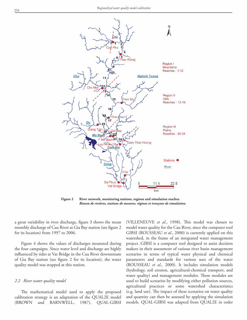
L. AUDET et al. / Revue des Sciences de l’Eau 31(3) (2018) 251-269 253
2. METHODOLOGY
2.1 Study area
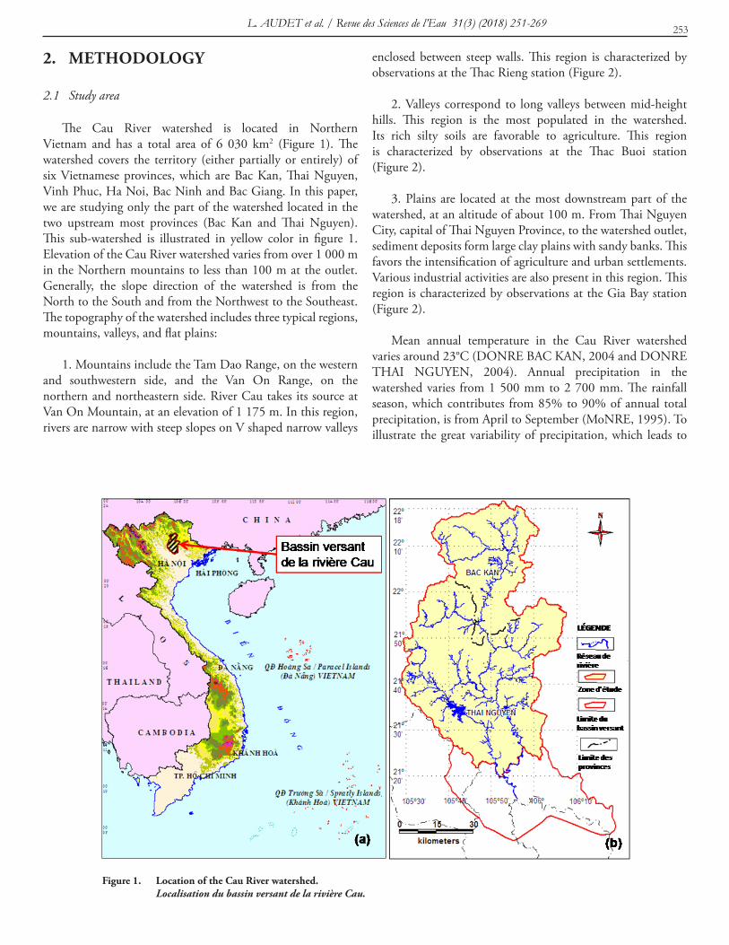
The Cau River watershed is located in Northern Vietnam and has a total area of 6 030 km2 (Figure 1). The watershed covers the territory (either partially or entirely) of six Vietnamese provinces, which are Bac Kan, Thai Nguyen, Vinh Phuc, Ha Noi, Bac Ninh and Bac Giang. In this paper, we are studying only the part of the watershed located in the two upstream most provinces (Bac Kan and Thai Nguyen). This sub-watershed is illustrated in yellow color in figure 1. Elevation of the Cau River watershed varies from over 1 000 m in the Northern mountains to less than 100 m at the outlet. Generally, the slope direction of the watershed is from the North to the South and from the Northwest to the Southeast. The topography of the watershed includes three typical regions, mountains, valleys, and flat plains:
1. Mountains include the Tam Dao Range, on the western and southwestern side, and the Van On Range, on the northern and northeastern side. River Cau takes its source at Van On Mountain, at an elevation of 1 175 m. In this region, rivers are narrow with steep slopes on V shaped narrow valleys
enclosed between steep walls. This region is characterized by observations at the Thac Rieng station (Figure 2).
2. Valleys correspond to long valleys between mid-height hills. This region is the most populated in the watershed. Its rich silty soils are favorable to agriculture. This region is characterized by observations at the Thac Buoi station (Figure 2).
3. Plains are located at the most downstream part of the watershed, at an altitude of about 100 m. From Thai Nguyen City, capital of Thai Nguyen Province, to the watershed outlet, sediment deposits form large clay plains with sandy banks. This favors the intensification of agriculture and urban settlements. Various industrial activities are also present in this region. This region is characterized by observations at the Gia Bay station (Figure 2).
Mean annual temperature in the Cau River watershed varies around 23°C (DONRE BAC KAN, 2004 and DONRE THAI NGUYEN, 2004). Annual precipitation in the watershed varies from 1 500 mm to 2 700 mm. The rainfall season, which contributes from 85% to 90% of annual total precipitation, is from April to September (MoNRE, 1995). To illustrate the great variability of precipitation, which leads to
Figure 1. Location of the Cau River watershed. Localisation du bassin versant de la rivière Cau.
Regionalized water quality model calibration254
Figure 2 River network, monitoring stations, regions and simulation reaches. Réseau de rivières, stations de mesures, régions et tronçons de simulation.
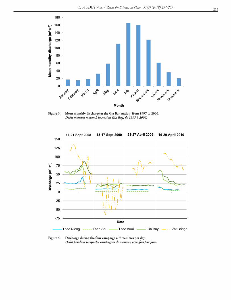
a great variability in river discharge, figure 3 shows the mean monthly discharge of Cau River at Gia Bay station (see figure 2 for its location) from 1997 to 2006.
Figure 4 shows the values of discharges measured during the four campaigns. Since water level and discharge are highly influenced by tides at Vat Bridge in the Cau River downstream of Gia Bay station (see figure 2 for its location), the water quality model was stopped at this station.
2.2 River water quality model
The mathematical model used to apply the proposed calibration strategy is an adaptation of the QUAL2E model (BROWN and BARNWELL, 1987), QUAL-GIBSI
(VILLENEUVE et al., 1998). This model was chosen to model water quality for the Cau River, since the computer tool GIBSI (ROUSSEAU et al., 2000) is currently applied on this watershed, in the frame of an integrated water management project. GIBSI is a computer tool designed to assist decision makers in their assessment of various river basin management scenarios in terms of typical water physical and chemical parameters and standards for various uses of the water (ROUSSEAU et al., 2000). It includes simulation models (hydrology, soil erosion, agricultural-chemical transport, and water quality) and management modules. These modules are used to build scenarios by modifying either pollution sources, agricultural practices or some watershed characteristics (e.g. land use). The impact of these scenarios on water quality and quantity can then be assessed by applying the simulation models. QUAL-GIBSI was adapted from QUAL2E in order
L. AUDET et al. / Revue des Sciences de l’Eau 31(3) (2018) 251-269 255
0
20
40
60
80
100
120
140
160
180
Mea
n m
ontlh
y di
scha
rge
(m3 ∙s
-1)
Month
-75
-50
-25
0
25
50
75
100
125
150
Dis
char
ge (m
3 ∙s-1
)
Date
Thac Rieng Than Sa Thac Buoi Gia Bay Vat Bridge
17-21 Sept 2008 13-17 Sept 2009 23-27 April 2009 16-20 April 2010
Figure 3. Mean monthly discharge at the Gia Bay station, from 1997 to 2006. Débit mensuel moyen à la station Gia Bay, de 1997 à 2006.
Figure 4. Discharge during the four campaigns, three times per day. Débit pendant les quatre campagnes de mesures, trois fois par jour.
Regionalized water quality model calibration256
to be compatible with the other simulation models in GIBSI and also to fulfill the requirements of integrated watershed management. The adaptations were to: 1) increase the maximal number of river reaches; 2) use the water flow variables (velocity, discharge, water height) simulated by the hydrological Hydrotel model (FORTIN et al., 2001), included in GIBSI; 3) add a dilution term in the advection-dispersion equation to allow the simulation of successive permanent states with varying discharge values (simulated with the Hydrotel model); 4) read new data concerning diffuse and point pollution sources at each time step; 5) modify the heat exchange module in order to take into account the exchanges between water and the river bed; 6) add the ROTO model (ARNOLD et al., 1995) to simulate stream deposition, bed erosion and sediment transport; 7) add the maximal number of non-conservative substances. Details concerning the equations of QUAL2E and QUAL-GIBSI can be found in BROWN and BARNWELL (1987) and VILLENEUVE et al. (1998) respectively.
2.3 Water quality data
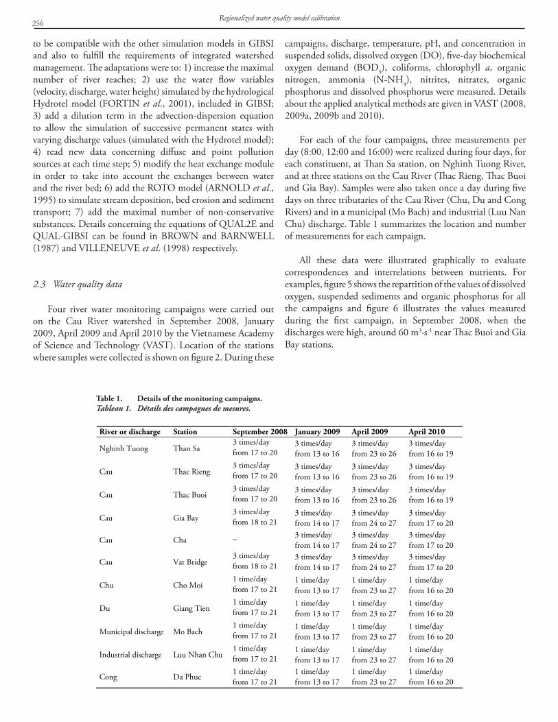
Four river water monitoring campaigns were carried out on the Cau River watershed in September 2008, January 2009, April 2009 and April 2010 by the Vietnamese Academy of Science and Technology (VAST). Location of the stations where samples were collected is shown on figure 2. During these
campaigns, discharge, temperature, pH, and concentration in suspended solids, dissolved oxygen (DO), five-day biochemical oxygen demand (BOD5), coliforms, chlorophyll a, organic nitrogen, ammonia (N-NH4), nitrites, nitrates, organic phosphorus and dissolved phosphorus were measured. Details about the applied analytical methods are given in VAST (2008, 2009a, 2009b and 2010).
For each of the four campaigns, three measurements per day (8:00, 12:00 and 16:00) were realized during four days, for each constituent, at Than Sa station, on Nghinh Tuong River, and at three stations on the Cau River (Thac Rieng, Thac Buoi and Gia Bay). Samples were also taken once a day during five days on three tributaries of the Cau River (Chu, Du and Cong Rivers) and in a municipal (Mo Bach) and industrial (Luu Nan Chu) discharge. Table 1 summarizes the location and number of measurements for each campaign.
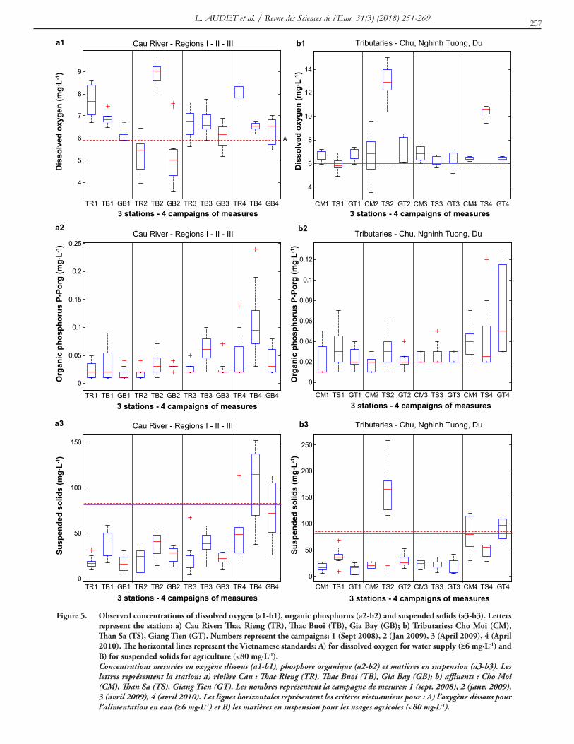
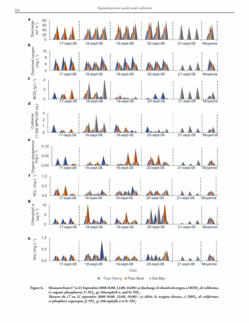
All these data were illustrated graphically to evaluate correspondences and interrelations between nutrients. For examples, figure 5 shows the repartition of the values of dissolved oxygen, suspended sediments and organic phosphorus for all the campaigns and figure 6 illustrates the values measured during the first campaign, in September 2008, when the discharges were high, around 60 m3∙s-1 near Thac Buoi and Gia Bay stations.
Table 1. Details of the monitoring campaigns.Tableau 1. Détails des campagnes de mesures.
River or discharge Station September 2008 January 2009 April 2009 April 2010
Nghinh Tuong Than Sa 3 times/day from 17 to 20
3 times/day from 13 to 16
3 times/day from 23 to 26
3 times/day from 16 to 19
Cau Thac Rieng 3 times/day from 17 to 20
3 times/day from 13 to 16
3 times/day from 23 to 26
3 times/day from 16 to 19
Cau Thac Buoi 3 times/day from 17 to 20
3 times/day from 13 to 16
3 times/day from 23 to 26
3 times/day from 16 to 19
Cau Gia Bay 3 times/day from 18 to 21
3 times/day from 14 to 17
3 times/day from 24 to 27
3 times/day from 17 to 20
Cau Cha –
3 times/day from 14 to 17
3 times/day from 24 to 27
3 times/day from 17 to 20
Cau Vat Bridge 3 times/day from 18 to 21
3 times/day from 14 to 17
3 times/day from 24 to 27
3 times/day from 17 to 20
Chu Cho Moi 1 time/day from 17 to 21
1 time/day from 13 to 17
1 time/day from 23 to 27
1 time/day from 16 to 20
Du Giang Tien 1 time/day from 17 to 21
1 time/day from 13 to 17
1 time/day from 23 to 27
1 time/day from 16 to 20
Municipal discharge Mo Bach 1 time/day from 17 to 21
1 time/day from 13 to 17
1 time/day from 23 to 27
1 time/day from 16 to 20
Industrial discharge Luu Nhan Chu 1 time/day from 17 to 21
1 time/day from 13 to 17
1 time/day from 23 to 27
1 time/day from 16 to 20
Cong Da Phuc 1 time/day from 17 to 21
1 time/day from 13 to 17
1 time/day from 23 to 27
1 time/day from 16 to 20
L. AUDET et al. / Revue des Sciences de l’Eau 31(3) (2018) 251-269 257
0
50
100
150
TR1 TB1 GB1 TR2 TB2 GB2 TR3 TB3 GB3 TR4 TB4 GB43 stations: 4 campagnes de mesure
Rivière Cau - Régions I - II - III
0
0.05
0.1
0.15
0.2
0.25
TR1 TB1 GB1 TR2 TB2 GB2 TR3 TB3 GB3 TR4 TB4 GB43 stations: 4 campagnes de mesure
4
5
6
7
8
9
TR1 TB1 GB1 TR2 TB2 GB2 TR3 TB3 GB3 TR4 TB4 GB4
A
4
6
8
10
12
14
CM1 TS1 GT1 CM2 TS2 GT2 CM3 TS3 GT3 CM4 TS4 GT43 stations: 4 campagnes de mesure
0
0.02
0.04
0.06
0.08
0.1
0.12
CM1 TS1 GT1 CM2 TS2 GT2 CM3 TS3 GT3 CM4 TS4 GT43 stations: 4 campagnes de mesure
Affluents - Chu, Nghinh Tuong, Du
0
50
100
150
200
250
CM1 TS1 GT1 CM2 TS2 GT2 CM3 TS3 GT3 CM4 TS4 GT43 stations: 4 campagnes de mesure
Affluents - Chu, Nghinh Tuong, Du
Dis
solv
ed o
xyge
n (m
g∙L-1
)O
rgan
ic p
hosp
horu
s P-
Porg
(mg∙
L-1)
Susp
ende
d so
lids
(mg∙
L-1)
Cau River - Regions I - II - III
Cau River - Regions I - II - III
3 stations - 4 campaigns of measures
3 stations - 4 campaigns of measures
Cau River - Regions I - II - III
3 stations - 4 campaigns of measures
3 stations - 4 campaigns of measures
3 stations - 4 campaigns of measures
3 stations - 4 campaigns of measures
Tributaries - Chu, Nghinh Tuong, Du
Tributaries - Chu, Nghinh Tuong, Du
Tributaries - Chu, Nghinh Tuong, Du
Dis
solv
ed o
xyge
n (m
g∙L-1
)O
rgan
ic p
hosp
horu
s P-
Porg
(mg∙
L-1)
Susp
ende
d so
lids
(mg∙
L-1)
b1
b2
b3a3
a2
a1
Figure 5. Observed concentrations of dissolved oxygen (a1-b1), organic phosphorus (a2-b2) and suspended solids (a3-b3). Letters represent the station: a) Cau River: Thac Rieng (TR), Thac Buoi (TB), Gia Bay (GB); b) Tributaries: Cho Moi (CM), Than Sa (TS), Giang Tien (GT). Numbers represent the campaigns: 1 (Sept 2008), 2 (Jan 2009), 3 (April 2009), 4 (April 2010). The horizontal lines represent the Vietnamese standards: A) for dissolved oxygen for water supply (≥6 mg∙L-1) and B) for suspended solids for agriculture (<80 mg∙L-1). Concentrations mesurées en oxygène dissous (a1-b1), phosphore organique (a2-b2) et matières en suspension (a3-b3). Les lettres représentent la station: a) rivière Cau : Thac Rieng (TR), Thac Buoi (TB), Gia Bay (GB); b) affluents : Cho Moi (CM), Than Sa (TS), Giang Tien (GT). Les nombres représentent la campagne de mesures: 1 (sept. 2008), 2 (janv. 2009), 3 (avril 2009), 4 (avril 2010). Les lignes horizontales représentent les critères vietnamiens pour : A) l’oxygène dissous pour l’alimentation en eau (≥6 mg∙L-1) et B) les matières en suspension pour les usages agricoles (<80 mg∙L-1).
Regionalized water quality model calibration258
4
6
8
10
Dis
solv
ed o
xyge
n(m
g·L-
1 )
17-sept-08 18-sept-08 19-sept-08 20-sept-08 21-sept-08 Moyenne
0
2
4
BOD
5 (g·
L-1 )
17-sept-08 18-sept-08 19-sept-08 20-sept-08 21-sept-08 Moyenne
0
1
2
3
Col
iform
s(1
000
MPN
/100
mL)
17-sept-08 18-sept-08 19-sept-08 20-sept-08 21-sept-08 Moyenne
0,00
0,05
0,10
Org
anic
pho
spho
rus
(mg·
L-1 )
17-sept-08 18-sept-08 19-sept-08 20-sept-08 21-sept-08 Moyenne
0,0
0,5
1,0
NO
3-(m
g·L-
1 )
17-sept-08 18-sept-08 19-sept-08 20-sept-08 21-sept-08 Moyenne
020406080
Dis
char
ge(m
3 ·s-
1 )
17-sept-08 18-sept-08 19-sept-08 20-sept-08 21-sept-08 Moyenne
0
5
10
Chl
orop
hyll
a (μ
g·L-
1 )
17-sept-08 18-sept-08 19-sept-08 20-sept-08 21-sept-08 Moyenne
0,0
0,5
1,0
NH
4+ (m
g ·L-1
)
19-sept-08
Thac Buoi Gia Bay
17-sept-08 18-sept-08 20-sept-08 21-sept-08 Moyenne
Thac Rieng
Date
Figure 6. Measures from 17 to 21 September 2008 (8:00, 12:00, 16:00): a) discharge, b) dissolved oxygen, c) BOD5, d) coliforms, e) organic phosphorus, f ) NO3, g) chlorophyll a, and h) NH4. Mesures du 17 au 21 septembre 2008 (8:00, 12:00, 16:00) : a) débit, b) oxygène dissous, c) DBO5, d) coliformes, e) phosphore organique, f) NO3, g) chlorophylle a et h) NH4.
a
b
c
d
e
f
g
h

L. AUDET et al. / Revue des Sciences de l’Eau 31(3) (2018) 251-269 259
2.4 Model implementation
Only the Cau River was included in the QUAL-GIBSI model for this application; the tributaries of the Cau River were considered as point loads in the model. The river was divided in 24 reaches, for a total of 125 km river length, as illustrated in figure 2. Water quality was simulated for 12 different days (18, 19 and 20 September 2008; 14, 15 and 16 January 2009; 24, 25 and 26 April 2009; 17, 18 and 19 April 2010). For each simulation day, river discharge must be given as input to the QUAL-GIBSI model, for each of the 24 river reaches. Since river discharge was measured at only a few monitoring stations during the monitoring campaigns, river discharges simulated by the Hydrotel model (FORTIN et al., 2001; calibrated for the Cau River watershed by NGUYEN (2012) were used as input for the 24 river reaches. Initial and limit conditions were determined based on five main assumptions listed below.
Assumption 1 concerns the spatial transposition of initial
concentrations. For reaches where the concentration of water quality constituents was measured three times per day, their daily means were applied as initial conditions. For reaches where no measurement was taken, the initial concentrations were set to the mean values measured at the stations located in the same region, where regions are defined as detailed in section 2.5. Assumption 2 concerns the weighting of initial concentrations at the confluence with important tributaries. For reaches located at the confluence with the Chu River, the Nghinh Tuong River and the Du River, the initial concentrations were estimated as the mean weighted value between concentrations in the tributary and in the Cau River, where the weights corresponded to the mean discharge in each river. Assumption 3 relates to the spatial transposition of loads coming from ungaged tributaries. Hydrological variables (discharge, water level and velocity) for the 23 tributaries included in the model were simulated with the Hydrotel model. For water quality however, concentrations are measured on only three tributaries (Chu, Nghinh Tuong and Du rivers). For the other 20 tributaries, the initial conditions for concentrations were set to the mean values measured in the gaged tributary located in the same region, where regions are defined as detailed in section 2.5. Assumption 4 deals with the computation of diffuse discharge along the river reaches. Those were computed from the Hydrotel model’s results, as the difference, for each reach, between the upstream and downstream discharge (from which, when applicable, the discharge of the tributary on this reach was subtracted). Finally, assumption 5 relates to diffuse loads. For these loads, concentrations were assumed to be equal to the mean daily observed concentrations in the Cau River.
2.5 Calibration and validation method
The applied calibration method consists of three main steps which are: 1) initial calibration; 2) sensitivity analysis; and 3) regional calibration. The simulated water variables are DO, BOD5, coliforms, chlorophyll a, organic nitrogen, N-NH4, nitrites, nitrates, organic phosphorus and dissolved phosphorus. The initial calibration was undertaken to provide parameter values to be used for sensitivity analysis. For both initial calibration and sensitivity analysis, parameters of the QUAL-GIBSI model were kept constant for all of the river reaches, while they varied between regions for the regional (final) calibration.
Three efficiency criteria were used to quantify the model performance for each day simulated during calibration and validation:
1. An objective function, Objv,i, that quantifies the relative difference between the observed and simulated values for each simulated water quality variable at each monitoring station, computed with:
ObjCs CmCmv iv i v i
v i,
, ,
,
=−
100 (1)
where i = 1, 2, or 3 respectively for the Thac Rieng, Thac Buoi and Gia Bay monitoring stations; Csv,i = mean simulated value per day and Cmv,i = mean measured value per day for 3 days of a monitoring campaign at station i for water quality variable v;
2. An objective function, Objv, that quantifies the relative difference between the observed and simulated values, averaged in absolute value over all 3 monitoring stations for each simulated water quality variable, computed with:
Obj
Cs CmCm
nv
v i v i
v ii
n
=
−
=∑ 1001
, ,
, (2)
where n = 3, number of monitoring station for a water quality variable v;
3. An objective function, Obj, that quantifies the overall performance per day of the model for the 3 monitoring station and the 10 simulated water quality variables, computed with:
Obj
Cs CmCm
nT
v i v i
v ii
n
v
T
=
−
=
=
∑∑
1001
1
, ,
, (3)
where T = 10, number of simulated water quality variables.

Regionalized water quality model calibration260
Finally, the results were compiled for three days during each campaign and their mean and standard deviation were calculated. Only the mean results for the two last criteria will be presented in this paper. One should note that a total of 270 measured data were used for the calibration process (3 stations * 3 monitoring campaigns * 3 days per campaign * 10 measured variables). Indeed, the ten water quality variables that are simulated are all connected in the equations of the model, so calibration cannot be performed in a sequential manner for each of the ten variables.
Initial calibration was based on the simulations and observations for September 2008, January 2009 and April 2009 monitoring campaigns. Some values of the parameters listed in table 2 were varied manually from their default values (taken from BROWN and BARNWELL, 1987) or from their mean value when a range is suggested in BROWN and BARNWELL (1987). All kinds of settling and decay rates, except BOD and nitrite decay rates (K1, β3), were set to zero during the initial calibration to minimize the impact of sedimentation; these parameters were adjusted further during the regional calibration. For F (fraction of algal nitrogen uptake from ammonium pool), initial value was set to 0.5 instead of 0.9. For the initial calibration, the O’CONNOR and DOBBINS (1958) equation was used to compute the reaeration rate K2 (option 3 in QUAL2E). The calibration was stopped when a better value of Obj could not be achieved.
Sensitivity analysis was performed by varying the parameter values by ±50% around a “mean” value which was either: 1) the value issued from initial calibration, for the parameters for which this value is different than zero (μ, ρ, α0, F); 2) for the parameters for which the value issued from initial calibration was equal to zero and for which BROWN and BARNWELL (1987) propose a range in the positive numbers domain, either the central value of this range (for σ1, σ4 and σ5) or a value chosen in such a way that all the parameter values used during the sensitivity analysis remained in this range (for K1, K5, β1, β2, β3 and β4); and 3) for the parameters for which the value issued from initial calibration was equal to zero and for which BROWN and BARNWELL (1987) propose a default value equal to zero (K4, σ2 and σ3), a value chosen to get a range of variation similar to those of the parameters representing similar processes. For the only parameter for which the range proposed by BROWN and BARNWELL (1987) covers negative and positive values (K3), only positive values were considered during sensitivity analysis. Finally, option 1 (values entered by the user) was used for the reaeration rate (K2) because it is the only option that allows manual variation of K2. Since the range of values proposed by BROWN and BARNWELL (1987) for K2 led to simulated DO values that were too far from the observed value, a mean value of 2 d-1 was used instead.
The relative variation of each water quality state variable was computed as a function of each of the 18 parameters listed in table 2 as follows:
∆v
v v
v
m
v v
v
Cs CsCs Cs Cs
Cs,% %
θ θ θθ
=
−
−=
−+ −
+ −
+ −
50 50 (4)
where ∆v ,θ = relative variation of water quality variable v as a function parameter θ; Csv+ = simulated value of water quality variable v with θ increased by 50% (all other parameters keeping their mean values); Csv- = simulated value of water quality variable v with θ decreased by 50% (all other parameters keeping their mean values); Csv = simulated value of water quality variable v with mean values for all parameters; θ+50% = mean value of parameter θ increased by 50%; θ-50% = mean value of parameter θ decreased by 50%; θm= mean value of parameter θ.
Results of the sensitivity analysis provided guidance for the final step of calibration, the regional calibration. This means that the parameters to which the results of the models were shown to be the most sensitive were those that were first varied during the calibration process. During this final calibration, three different set of parameters’ values were defined. Once again, the calibration was performed based on the Obj value (see equation 3) and was stopped when a better value for Obj could not be achieved. Each of the three sets of parameters was used in a specific region. Regions were delimited based on topography and land use. The three monitoring stations are representative of each region, since they reflect the diversity in land use and topography encountered throughout the watershed. The three regions are identified as I, II and III in figure 2 and their main characteristics are given in table 3.
As for the initial calibration, the regional calibration was based on the simulations and observations for the September 2008, January 2009 and April 2009 monitoring campaigns (Figures 5 and 6). Finally, validation of the calibrated model was performed based on the simulations and observations for April 2010 monitoring campaigns, with simulated values obtained using the parameters’ values issued from the regional calibration.
For the regional calibration and the validation, the reaeration rate, K2, was computed using the equation developed by CHURCHILL et al. (1962) (option 2 in QUAL2E). Indeed, it was found that this equation allowed a better representation of the spatial variations in DO concentration. Consequently, for initial calibration, the value of 17 parameters had to be estimated, while for regional calibration, 51 parameter values (17 parameters * 3 stations) were estimated.
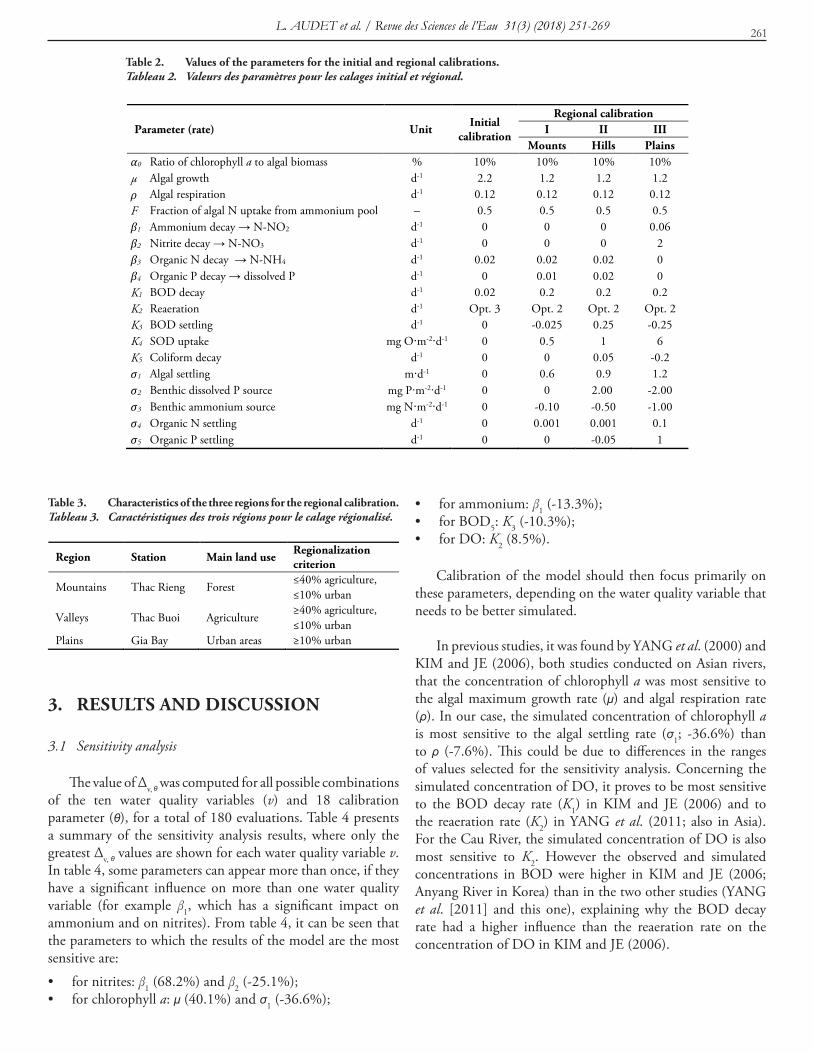
L. AUDET et al. / Revue des Sciences de l’Eau 31(3) (2018) 251-269 261
Parameter (rate) Unit Initial calibration
Regional calibration I II III
Mounts Hills Plains α0 Ratio of chlorophyll a to algal biomass % 10% 10% 10% 10% µ Algal growth d-1 2.2 1.2 1.2 1.2 ρ Algal respiration d-1 0.12 0.12 0.12 0.12 F Fraction of algal N uptake from ammonium pool – 0.5 0.5 0.5 0.5 β1 Ammonium decay → N-NO2 d-1 0 0 0 0.06 β2 Nitrite decay → N-NO3 d-1 0 0 0 2 β3 Organic N decay → N-NH4 d-1 0.02 0.02 0.02 0 β4 Organic P decay → dissolved P d-1 0 0.01 0.02 0 K1 BOD decay d-1 0.02 0.2 0.2 0.2 K2 Reaeration d-1 Opt. 3 Opt. 2 Opt. 2 Opt. 2 K3 BOD settling d-1 0 -0.025 0.25 -0.25 K4 SOD uptake mg O∙m-2∙d-1 0 0.5 1 6 K5 Coliform decay d-1 0 0 0.05 -0.2 σ1 Algal settling m∙d-1 0 0.6 0.9 1.2 σ2 Benthic dissolved P source mg P∙m-2∙d-1 0 0 2.00 -2.00 σ3 Benthic ammonium source mg N∙m-2∙d-1 0 -0.10 -0.50 -1.00 σ4 Organic N settling d-1 0 0.001 0.001 0.1 σ5 Organic P settling d-1 0 0 -0.05 1
Table 2. Values of the parameters for the initial and regional calibrations.Tableau 2. Valeurs des paramètres pour les calages initial et régional.
Table 3. Characteristics of the three regions for the regional calibration.Tableau 3. Caractéristiques des trois régions pour le calage régionalisé.
3. RESULTS AND DISCUSSION
3.1 Sensitivity analysis
The value of Δv, θ was computed for all possible combinations of the ten water quality variables (v) and 18 calibration parameter (θ), for a total of 180 evaluations. Table 4 presents a summary of the sensitivity analysis results, where only the greatest Δv, θ values are shown for each water quality variable v. In table 4, some parameters can appear more than once, if they have a significant influence on more than one water quality variable (for example β1, which has a significant impact on ammonium and on nitrites). From table 4, it can be seen that the parameters to which the results of the model are the most sensitive are:
• for nitrites: β1 (68.2%) and β2 (-25.1%);• for chlorophyll a: μ (40.1%) and σ1 (-36.6%);
• for ammonium: β1 (-13.3%);• for BOD5: K3 (-10.3%);• for DO: K2 (8.5%).
Calibration of the model should then focus primarily on these parameters, depending on the water quality variable that needs to be better simulated.
In previous studies, it was found by YANG et al. (2000) and KIM and JE (2006), both studies conducted on Asian rivers, that the concentration of chlorophyll a was most sensitive to the algal maximum growth rate (μ) and algal respiration rate (ρ). In our case, the simulated concentration of chlorophyll a is most sensitive to the algal settling rate (σ1; -36.6%) than to ρ (-7.6%). This could be due to differences in the ranges of values selected for the sensitivity analysis. Concerning the simulated concentration of DO, it proves to be most sensitive to the BOD decay rate (K1) in KIM and JE (2006) and to the reaeration rate (K2) in YANG et al. (2011; also in Asia). For the Cau River, the simulated concentration of DO is also most sensitive to K2. However the observed and simulated concentrations in BOD were higher in KIM and JE (2006; Anyang River in Korea) than in the two other studies (YANG et al. [2011] and this one), explaining why the BOD decay rate had a higher influence than the reaeration rate on the concentration of DO in KIM and JE (2006).
Region Station Main land use Regionalization criterion
Mountains Thac Rieng Forest ≤40% agriculture, ≤10% urban
Valleys Thac Buoi Agriculture ≥40% agriculture, ≤10% urban
Plains Gia Bay Urban areas ≥10% urban
Regionalized water quality model calibration262
State variable Parameter (rate) Unit Minimum value
Mean value
Maximum value
Δv, 2 (%)
DO K2 Reaeration d-1 1 2 3 8.5 K4 SOD uptake mg O∙m-2∙d-1 1 2 3 -3.4
BOD5 K3 BOD settling d-1 0.1 0.2 0.3 -10.3 K1 BOD decay d-1 0.02 0.04 0.06 -2.3
Coliforms K5 Coliform decay d-1 0.05 0.1 0.15 -5.8 Chlorophyll a µ Algal growth d-1 1.1 2.2 3.3 40.1
σ1 Algal settling m∙d-1 1 2 3 -36.6 ρ Algal respiration d-1 0.06 0.12 0.18 -7.6 α0 Ratio of chlorophyll a to algal biomass % 5% 10% 15% 0.8
Organic N σ4 Organic N settling d-1 0.025 0.05 0.075 -2.6 β3 Organic N decay → N-NH4 d-1 0.02 0.04 0.06 -2.3
Ammonium N-NH4
β3 Organic N decay → N-NH4 d-1 0.02 0.04 0.06 3.3 β1 Ammonium decay → N-NO2 d-1 0.1 0.2 0.3 -13.3 σ3 Benthic ammonium source mg N∙m-2∙d-1 0.025 0.05 0.075 0.01
Nitrites N-NO2
β1 Ammonium decay → N-NO2 d-1 0.1 0.2 0.3 68.2 β2 Nitrite decay → N-NO3 d-1 0.2 0.4 0.6 -25.1
Nitrates N-NO3
β2 Nitrite decay → N-NO3 d-1 0.2 0.4 0.6 1.0 F Fraction of algal nitrogen uptake from
ammonium pool N-NH4 / (N-NH4 + N-NO3)
– 0.25 0.5 0.75 1.0
Organic P σ5 Organic P settling d-1 0.025 0.05 0.075 -2.7 β4 Organic P decay → dissolved P d-1 0.01 0.02 0.03 -1.2
Dissolved P β4 Organic P decay → dissolved P d-1 0.01 0.02 0.03 2.8 σ2 Benthic dissolved P source mg P∙m-2∙d-1 0.025 0.05 0.075 1.1
Table 4. Data and results of the sensitivity analysis.Tableau 4. Données et résultats de l’analyse de sensibilité.
3.2 Calibration and validation
Table 2 presented before gives the values of the parameters issued from the initial and regional calibrations, while table 5 presents the results of both calibrations as well as of validation. As mentioned before, the state variables were simulated for nine different days during both calibrations (18, 19 and 20 September 2008; 14, 15 and 16 January 2009; 24, 25 and 26 April 2009) and for three days during validation (17, 18 and 19 April 2010). The values in table 5 are the mean values of the objective function averaged over these days and over the three monitoring stations, while the errors presented (following the symbol “±”) are the standard deviations between these values. Good values are those for which both the mean value of Obj (or Objv) and its standard deviation are low. Figures 7 and 8 show some simulation results for chlorophyll a, N-NO2, organic P and dissolved P. Complete results for all simulated state variables are given in AUDET (2013).
Results in table 5 (as well as in figures 7 and 8) show that the calibration results are significantly improved by applying regionalization as compared to the initial calibration for all simulated state variables, except for BOD5 and coliforms for which the calibration are similar between the initial and regional
State variable Initial calibration
Regional calibration Validation
Objective value averaged over the three monitoring stations (Objv) DO 11 ± 7 7 ± 5 9 ± 2 BOD5 12 ± 12 14 ± 8 13 ± 2 Coliforms 21 ± 15 21 ± 14 39 ± 27 Chlorophyll a 49 ± 27 15 ± 11 9 ± 4 Organic N 8 ± 5 7 ± 4 6 ± 1 Ammonium N-NH4
12 ± 7 11 ± 6 13 ± 2
Nitrites N-NO2 86 ± 245 27 ± 58 16 ± 4 Nitrates N-NO3 6 ± 3 5 ± 3 9 ± 2 Organic P 23 ± 18 9 ± 8 10 ± 1 Dissolved P 19 ± 12 10 ± 8 5 ± 0
Mean objective averaged over the three monitoring stations (Obj)
25 ± 25 13 ± 6 13 ± 2
Table 5. Calibration and validation results.Tableau 5. Résultats de calage et de validation.

L. AUDET et al. / Revue des Sciences de l’Eau 31(3) (2018) 251-269 263
0123456
0 4 8 12 16 20 24
Chl
orop
hyll
a(μ
g·L-
1 )19 September 2008
0123456
0 4 8 12 16 20 24
Chl
orop
hyll
a(μ
g·L-
1 )
15 January 2009
0123456
0 4 8 12 16 20 24
Chl
orop
hyll
a(μ
g·L-
1 )
25 April 2009
0123456
0 4 8 16 20 24
Chl
orop
hyll
a(μ
g·L-
1 )
18 April 2010
Regionalised calibration
12
ReachObservationsIniatial calibration
0,0
0,5
1,0
0 4 8 12 16 20 24
N-N
O2
(mg·
L-1 ) 19 September 2008
0,0
0,5
1,0
0 4 8 12 16 20 24
N-N
O2
(mg·
L-1 ) 15 January 2009
0,00,20,40,60,81,0
0 4 8 12 16 20 24N
-NO
2(m
g·L-
1 ) 25 April 2009
0,0
0,5
1,0
0 4 8 12 16 20 24
N-N
O2
(mg·
L-1 ) 18 April 2010
Regionalised calibration
Reach
ObservationsInitial calibration
Figure 7. Examples of simulation results for chlorophyll a and N-NO2. Exemples de résultats de simulation pour la chlorophylle a et le N-NO2.
calibrations. Overall, the mean objective function (averaged over all state variables) is significantly better in regional that in initial calibration. Use of the parameters obtained from the regional calibration also leads to good results during the validation period. Improvements of the results from the initial to the regional calibration are mainly due to the variation of the parameters between the three regions, which allows taking into account the differences between the regions in terms of topography and land use.
The variations of the parameter values among the three regions, in the regional calibration, are dictated by differences in land use and physiographic characteristics. For each region, some parameters can also be adjusted in order to reproduce processes that are not explicitly modeled in QUAL2E. As for example, the concentration of coliforms in QUAL2E is modeled as a simple first order decay reaction, without any interaction with the other water quality variables. However, it is well known that high concentrations of coliforms can lead to
reductions in dissolved oxygen concentrations (see for example DAVIES-COLLEY et al., 1999, or figure 6). To take this into account, variations in the value of K4, the sediment oxygen demand (SOD) uptake rate, can represent real variations in SOD, but also the variations of oxygen demand for the degradation of coliforms, or for any other oxygen demanding process. This is why the value of K4 for the final calibration is higher in Region III that in the two other regions, to reproduce the oxygen demand from coliforms in this urbanized area.
All other calibration parameters can be similarly adjusted as a function of land use and topographical characteristics in each region. Thus σ1, the algal settling rate, was given increasing values from Region I to Region III, due to decreasing water velocity (decreasing river slopes) from upstream to downstream. For the same reason, coliforms travel rapidly in Region I, leading to rapid variations in coliforms concentrations in this area. The variation of these concentrations in Region I can thus be modeled based only on water transport, without taking
Regionalized water quality model calibration264
0,000,020,040,060,080,10
0 4 8 12 16 20 24
P org
(mg·
L-1 ) 19 September 2008
0,00
0,05
0,10
0 4 8 12 16 20 24
P org
(mg·
L-1 ) 15 January 2009
0,000,020,040,060,080,10
0 4 8 12 16 20 24
P org
(mg·
L-1 ) 25 April 2009
0,00
0,05
0,10
0 4 8 12 16 20 24
P org
(mg·
L-1 )
Reach
18 April 2010
Regionalised calibration Initial calibration Observations
0,00
0,02
0,04
0,06
0 4 8 12 16 20 24
P dis
s(m
g·L-
1 ) 19 September 2008
0,00
0,02
0,04
0,06
0 4 8 12 16 20 24
P dis
s(m
g·L-
1 ) 15 January 2009
0,00
0,02
0,04
0,06
0 4 8 12 16 20 24P d
iss
(mg·
L-1 ) 25 April 2009
0,000,010,020,030,040,050,06
0 4 8 12 16 20 24
P dis
s(m
g·L-
1 )
Reach
18 April 2010
Regionalised calibration Initial calibration Observations
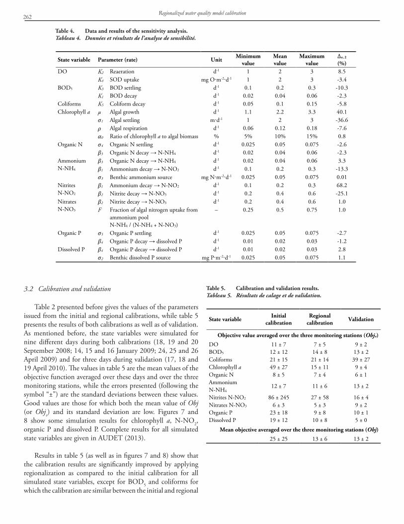
Figure 8. Examples of simulation results for organic and dissolved phosphorus. Exemples de résultats de simulation pour le phosphore organique et dissous.
into account a mortality rate (hence a value of 0 d-1 for K5, the coliform decay rate, in Region I). In Region II, water velocities are lower and a decay rate is required to reproduce the self-purification capacity of the river (K5 = 0.05 d-1). In Region III, massive coliform inputs are brought by the Du River and by untreated municipal wastewater discharges. These inputs most often exceed the self-purification capacity of the river, hence a negative rate of -0.2 d-1 for K5 in the urbanized region (Region III).
As for dissolved phosphorus, the benthic source was set to 0 mg P∙m-2 d-1 in Region I, due to the low sedimentation rate in the mountainous area, while in Region II, mostly agricultural, the bio-dynamism could foster a higher P contribution from benthos (σ2 = 2 mg P∙m-2∙d-1). In Region III, benthos is largely affected by industrial and municipal wastewater discharges, which could lead to decrease in the benthic contribution to dissolved phosphorus. Moreover, the high dissolved P contribution from untreated wastewater discharges in this
region combined with low river flow velocities cause a net loss from dissolved P from the water column to the sediments, hence a negative value for σ2 in Region III (-2 mg P∙m-2∙d-1).
Concerning σ5, the settling rate of organic P, it was set to 0 d-1 in the upstream region since sedimentation is very low, if not absent, in this part of the river, and in order to favor the transport of organic matter to the agricultural valleys. At Thac Buoi, organic phosphorus concentrations are very high, often from two to four times higher than the concentrations upstream and downstream (see figure 8). This can be observed in all seasons and could be due to the release of organic phosphorus from the agricultural lands, either from rice fields or directly from the sedimentary deposits that are highly biologically active. This is why a negative value was given to σ5 in the central region (σ5 = -0.05 d-1), reflecting a benthic contribution in organic phosphorus in this agricultural area. Some studies have shown that organic phosphorus can be transported with suspended sediments (e.g. SHEN et al., 2008)
L. AUDET et al. / Revue des Sciences de l’Eau 31(3) (2018) 251-269 265
and this is what was observed for the Cau River in January (see figure 5). Observations at Thac Buoi show the importance of the organic phosphorus availability in this agricultural region rich in alluvium. At Gia Bay, the concentrations of organic phosphorus are generally lower. It can be presumed that the settling rate of organic P is very high in this region (a value of σ5 = 1 d-1 was chosen) due to the deposition of suspended sediments in this region where the river flow velocity is reduced.
Many local reports mention ammonia odors along the riverbank near Gia Bay. Moreover, denitrification, and thus production of nitrogen gas N2, could occur in this area when concentrations in dissolved oxygen are low. This means that there could be a net loss of nitrogen to the atmosphere, which is not taken into account in the model. Indeed, in QUAL2E and QUAL-GIBSI, the denitrification process is not simulated, but the nitrification module is stopped when concentrations in dissolved oxygen are low. To take this into account, negative values were given to σ3, the benthic ammonium source rate in the three regions (-0.1 mg N∙m-2∙d-1 in Region I, -0.5 mg N∙m-2∙d-1 in Region II, and 1 mg N∙m-2∙d-1 in Region III). Negative values of σ3 allow to reproduce nitrogen losses in the model, losses that could occur either by deposition of suspended solids or by ammonia or N2 losses to the atmosphere.
Finally, for the calibration of σ4, the settling rate of organic N, it was assumed to be minimal upstream (σ4 = 0.001 d-1 in Region I) and maximal downstream (σ4 = 0.1 d-1 in Region III) according to the physical characteristics of each environment. However, in Region II, input loads from agriculture could counterbalance the deposition rate and thus a minimal value for σ4 was retained (σ4 = 0.001 d-1 in Region II).
All these considerations show how a comprehensive study of land use and land physical characteristics, in conjunction with observed data, can help to estimate the regional values of the model’s parameters. This approach could be beneficial for river water quality modelling on any type of watershed, and especially on those where observed data are too scarce to describe all the dynamics related to water quality, like often encountered in developing countries. It also shows how a judicious definition of the value of some parameters allows reproducing processes that are not explicitly represented in the model (e.g. oxygen demand for the degradation of coliforms, denitrification and production of nitrogen gas).
4. CONCLUSION
A novel methodology for the calibration of water quality simulation models, which applies to large watersheds where intensive measurements for water quality and quantity are
lacking, was proposed in this paper. The methodology is based on: 1) the use of the results from a hydrological model to provide the required hydrological variables (discharge, water level and velocity) to the water quality model; 2) five assumptions for the definition of initial and boundary conditions; 3) a three-step regionalized calibration method, in which the specific characteristics of the different subwatersheds are taken into account and 4) the adjustment of some parameters in order to reproduce processes that are not explicitly represented in the model. The methodology was applied, as a test case study, to the Cau River in Vietnam. As compared to most of the calibration studies that were previously conducted on river water quality models with optimization algorithms, the proposed procedure relies on a comprehensive study of the land use and characteristics on each subwatershed and the definition of different sets of parameters values in distinct regions. For the specific case of the Cau River, the sensitivity analysis, that is part of the calibration method, showed that the parameters to which the model’s results are the most sensitive are: β1 and β2 for nitrites; μ and σ1 for chlorophyll a; β1 for ammonium; K3 for BOD5; and K2 for DO. These results could guide future calibration work for river water quality models in the South East Asia Region, or in any other watershed experiencing a tropical monsoon climate. Application of the methodology to the Cau River also showed that calibration and validation results were significantly improved by applying regionalization as compared to an initial calibration for which a single set of parameters values was used for the whole simulated river stretch. Furthermore, use of the results from a hydrological model to provide the required hydrological variables to the water quality model demonstrates how integrated modeling systems at the watershed scale, by combining different simulation models, can be beneficially applied on watersheds where observed data are scarce. When integrated in such an integrated modeling system, the river water quality model, once calibrated, can be used in conjunction with other simulation models at the watershed scale (as for example, pollutant and/or sediment production and transport models) to assess the impacts of various potential future interventions on the river water quality.
ACKNOWLEDGMENTS
This work was conducted within the context of the cooperative research project ‘‘Cau River basin integrated management’’ between Institut national de la recherche scientifique (INRS, Canada) and Vietnam Academy of Science and Technology (VAST), funded by the Canadian International Development Agency (CIDA; project 612-T203-05). The authors would like to thank the support from this project and from the VAST project 07.02/13-14. The authors also wish to thank the project’s staff for supporting data collection and sharing information.
Regionalized water quality model calibration266
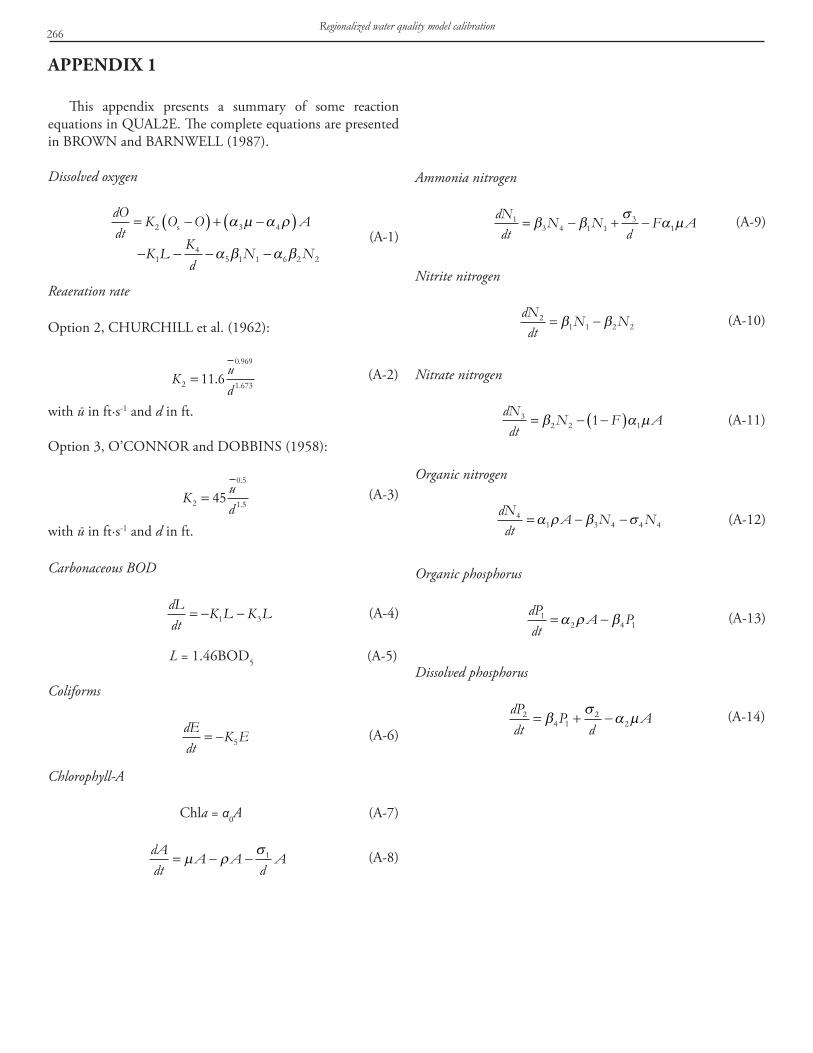
APPENDIX 1
This appendix presents a summary of some reaction equations in QUAL2E. The complete equations are presented in BROWN and BARNWELL (1987).
Dissolved oxygen
dOdt
K O O A
K L Kd
N N
= −( ) + −( )
− − − −
2 3 4
14
5 1 1 6 2 2
s α µ α ρ
α β α β (A-1)
Reaeration rate
Option 2, CHURCHILL et al. (1962):
K ud2
0 969
1 67311 6= ..
. (A-2)
with ū in ft∙s-1 and d in ft.
Option 3, O’CONNOR and DOBBINS (1958):
K ud2
0 5
1 545=.
. (A-3)
with ū in ft∙s-1 and d in ft.
Carbonaceous BOD
dLdt
K L K L= − −1 3 (A-4)
L = 1.46BOD5 (A-5)
Coliforms
dEdt
K E= − 5 (A-6)
Chlorophyll-A
Chla = α0A (A-7)
dAdt
A AdA= − −µ ρ
σ1 (A-8)
Ammonia nitrogen
dNdt
N Nd
F A13 4 1 1
31= − + −β β
σα µ (A-9)
Nitrite nitrogen
dNdt
N N21 1 2 2= −β β (A-10)
Nitrate nitrogen
dNdt
N F A32 2 11= − −( )β α µ (A-11)
Organic nitrogen
dNdt
A N N41 3 4 4 4= − −α ρ β σ (A-12)
Organic phosphorus
dPdt
A P12 4 1= −α ρ β (A-13)
Dissolved phosphorus
dPdt
Pd
A24 1
22= + −β
σα µ (A-14)
L. AUDET et al. / Revue des Sciences de l’Eau 31(3) (2018) 251-269 267
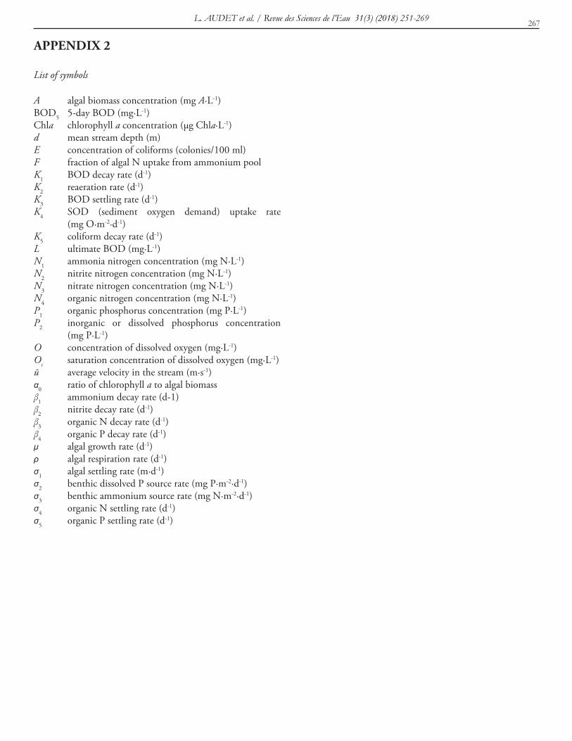
APPENDIX 2
List of symbols
A algal biomass concentration (mg A∙L-1)BOD5 5-day BOD (mg∙L-1)Chla chlorophyll a concentration (µg Chla∙L-1)d mean stream depth (m)E concentration of coliforms (colonies/100 ml)F fraction of algal N uptake from ammonium pool K1 BOD decay rate (d-1)K2 reaeration rate (d-1)K3 BOD settling rate (d-1)K4 SOD (sediment oxygen demand) uptake rate
(mg O∙m-2∙d-1)K5 coliform decay rate (d-1)L ultimate BOD (mg∙L-1)N1 ammonia nitrogen concentration (mg N∙L-1)N2 nitrite nitrogen concentration (mg N∙L-1)N3 nitrate nitrogen concentration (mg N∙L-1)N4 organic nitrogen concentration (mg N∙L-1)P1 organic phosphorus concentration (mg P∙L-1)P2 inorganic or dissolved phosphorus concentration
(mg P∙L-1)O concentration of dissolved oxygen (mg∙L-1)Os saturation concentration of dissolved oxygen (mg∙L-1)ū average velocity in the stream (m∙s-1)α0 ratio of chlorophyll a to algal biomassβ1 ammonium decay rate (d-1)β2 nitrite decay rate (d-1)β3 organic N decay rate (d-1)β4 organic P decay rate (d-1)μ algal growth rate (d-1)ρ algal respiration rate (d-1)σ1 algal settling rate (m∙d-1)σ2 benthic dissolved P source rate (mg P∙m-2∙d-1)σ3 benthic ammonium source rate (mg N∙m-2∙d-1)σ4 organic N settling rate (d-1)σ5 organic P settling rate (d-1)

Regionalized water quality model calibration268
REFERENCES
ARNOLD J.G., J.R. WILLIAMS and D.R. MAIDMENT (1995). Continuous-time water and sediment-routing model for large basins. J. Hydraul. Eng., 121, 171-183.
AUDET L. (2013). Modélisation de la qualité de l’eau de la rivière Cau au Vietnam. Master's thesis. Univ. Québec, INRS, Canada, 176 p.
BERBER R., M. YUCEER and E. KARADURMUS (2009). A parameter identifiability and estimation study in Yesilirmak River. Water Sci. Tech., 59, 515-521.
BROWN L.C. and T.O. BARNWELL JR. (1987). The enhanced stream water quality models QUAL2E and QUAL2E-UNCAS: Documentation and user manual. US Environmental Protection Agency, EPA-600/3-87/007, Athens (GA), USA, 189 p.
CHAPRA S.C., G.J. PELLETIER and H. TAO (2007). QUAL2K: A Modeling framework for simulating river and stream water quality, version 2.07, Documentation and user’s manual. Civil and Environmental Engineering Department, Tufts University, Medford (MA), USA, 97 p.
CHO H.C. and S.R. HA (2010). Parameter optimization of the QUAL2K model for a multiple-reach river using an influence coefficient algorithm. Sci. Total Environ., 408, 1985-1991.
CHURCHILL M.A., H.L ELMORE and R.A. BUCKINGHAM (1962). The prediction of stream reaeration rates. Int. J. Air Water Pollut., 6, 467-504.
COX B.A. (2003). A review of currently available in-stream water-quality models and their applicability for simulating dissolved oxygen in lowland rivers. Sci. Total Environ., 314-316, 335-377.
DAVIES-COLLEY R.J., A.M. DONNISON, D.J. SPEED, C.M. ROSS and J.W. NAGELS (1999). Inactivation of faecal indicator microorganisms in waste stabilisation ponds: interactions of environmental factors with sunlight. Water Res., 33, 1220-1230.
DEPARTMENT OF NATURAL RESOURCES AND ENVIRONMENT (DONRE BAC KAN) (2004). Annual report on environmental status of the Bac Kan Province. Bac Kan, Vietnam.
DEPARTMENT OF NATURAL RESOURCES AND ENVIRONMENT (DONRE THAI NGUYEN) (2004). Annual report on environmental status of the Thai Nguyen Province. Thai Nguyen, Vietnam.
FORTIN J.P., R. TURCOTTE, S. MASSICOTTE, R. MOUSSA, J. FITZBACK and J.P. VILLENEUVE (2001). Distributed watershed model compatible with remote sensing and GIS data. I: Description of model. J. Hydrol. Eng., 6, 91-99.
HA P.T.T., N. KOKUTSE, S. DUCHESNE, J.P. VILLENEUVE, A. BÉLANGER, H.N. HIEN, B. TOUMBOU and D.N. BACH (2017). Assessing and selecting interventions for river water quality improvement within the context of population growth and urbanization: A case study of the Cau River Basin in Vietnam. Environ. Dev. Sustain., 19, 1701-1729.
KARADURMUS E. and R. BERBER (2004). Dynamic simulation and parameter estimation in river streams. Environ. Technol., 25, 471-479.
KIM K.S. and C.H. JE (2006). Development of a framework of automated water quality parameter optimization and its application. Environ. Geol., 49, 405-412.
MINISTRY OF NATURAL RESOURCES AND ENVIRONMENT (MONRE) (1995). Át lát khí tượng thủy văn quốc gia (National Hydro-Meteorological Atlas, in Vietnamese). Hanoi, Vietnam, 76 p.
NG A.W.N. and B.J.C. PERERA (2003). Selection of genetic algorithm operators for river water quality model calibration. Eng. Appl. Artif. Intell., 16, 529-541.
NGUYEN H.T. (2012). Apport de la modélisation hydrologique distribuée à la gestion intégrée par bassin versant des ressources en eau. Ph.D. thesis, Univ. Québec, INRS, Canada, 180 p.
O’CONNOR D.J., and W.E. DOBBINS (1958). Mechanism of reaeration in natural stream. Transactions ASCE, 123, 641-684.
REICHERT P., D. BORCHARDT, M. HENZE, W. RAUCH, P. SHANAHAN, L. SOMLYÓDY and P. VANROLLEGHEM (2001). River Water Quality Model no. 1 (RWQM1). II. Biochemical process equations. Water Sci. Technol., 43, 11-30.
L. AUDET et al. / Revue des Sciences de l’Eau 31(3) (2018) 251-269 269
ROUSSEAU A.N., A. MAILHOT, R. TURCOTTE, M. DUCHEMIN, C. BLANCHETTE, M. ROUX, N. ETONG, J. DUPONT and J.P. VILLENEUVE (2000). GIBSI - An integrated modelling system prototype for river basin management. Hydrobiologia, 422/423, 465-475.
SHEN Z., Q. HONG, H. YU and R. LIU (2008). Parameter uncertainty analysis of the non-point source pollution in the Daning River watershed of the Three Gorges Reservoir Region, China. Sci. Total Environ., 405, 195-205.
STREETER A.W. and E.B. PHELPS (1925). A study of the pollution and natural purification of the Ohio River, III. Factors concerned in the phenomena of oxidation and reaeration. US Public Health Bulletin 146, US Public Health Service, Washington (DC), USA, 75 p.
VIETNAMESE ACADEMY OF SCIENCE AND TECHNOLOGY (VAST) (2008). Report on water quality monitoring for Cau River - Project on integrated Cau River basin management, Hanoi, Vietnam: First time - from 17 to 21 September, 2008. Institute of Environmental Technology, Hanoi, Vietnam, 18 p.
VIETNAMESE ACADEMY OF SCIENCE AND TECHNOLOGY (VAST) (2009a). Report on water quality monitoring for Cau River - Project on integrated Cau River basin management, Hanoi, Vietnam: Second time - from 14 to 17 January, 2009. Institute of Environmental Technology, Hanoi, Vietnam, 19 p.
VIETNAMESE ACADEMY OF SCIENCE AND TECHNOLOGY (VAST) (2009b). Report on water quality monitoring for Cau River - Project on integrated Cau River basin management, Hanoi, Vietnam - From 23 April to 27 April, 2009. Institute of Environmental Technology, Hanoi, Vietnam, 19 p.
VIETNAMESE ACADEMY OF SCIENCE AND TECHNOLOGY (VAST) (2010). Report on water quality monitoring for Cau River - Project on integrated Cau River basin management, Hanoi, Vietnam - From 16 April to 20 April, 2010. Institute of Environmental Technology, Hanoi, Vietnam, 19 p.
VILLENEUVE J.P., C. BLANCHETTE, M. DUCHEMIN, J.F. GAGNON, A. MAILHOT, A.N. ROUSSEAU, M. ROUX, J.F. TREMBLAY et R. TURCOTTE (1998). Rapport final du projet GIBSI : gestion de l’eau des bassins versants à l’aide d’un système informatisé - Tome 1. Research report R-462, INRS, Centre Eau Terre Environnement, Québec (QC), Canada, 371 p.
YANG C.C., C.S. CHEN and C.S. LEE (2011). Comprehensive river water quality management by simulation and optimization models. Environ. Model. Assess., 16, 283-294.
YANG M.D., R.M. SYKES and C.J. MERRY (2000). Estimation of algal biological parameters using water quality modeling and SPOT satellite data. Ecol. Modell., 125, 1-13.