HAL Id: hal-02081485https://hal.archives-ouvertes.fr/hal-02081485v3

Submitted on 24 Sep 2019

HAL is a multi-disciplinary open accessarchive for the deposit and dissemination of sci-entific research documents, whether they are pub-lished or not. The documents may come fromteaching and research institutions in France orabroad, or from public or private research centers.

L’archive ouverte pluridisciplinaire HAL, estdestinée au dépôt et à la diffusion de documentsscientifiques de niveau recherche, publiés ou non,émanant des établissements d’enseignement et derecherche français ou étrangers, des laboratoirespublics ou privés.

A reduced basis method for parametrized variationalinequalities applied to contact mechanics

Amina Benaceur, Alexandre Ern, Virginie Ehrlacher

To cite this version:Amina Benaceur, Alexandre Ern, Virginie Ehrlacher. A reduced basis method for parametrized vari-ational inequalities applied to contact mechanics. International Journal for Numerical Methods inEngineering, Wiley, 2019, 10.1002/nme.6261. hal-02081485v3

A reduced basis method for parametrized variationalinequalities applied to contact mechanics∗

Amina Benaceur†‡, Alexandre Ern†, Virginie Ehrlacher†

Abstract

We investigate new developments of the Reduced-Basis (RB) method for parametrized opti-mization problems with nonlinear constraints. We propose a reduced-basis scheme in a saddle-point form combined with the Empirical Interpolation Method to deal with the nonlinear con-straint. In this setting, a primal reduced-basis is needed for the primal solution and a dualone is needed for the Lagrange multipliers. We suggest to construct the latter using a cone-projected greedy algorithm that conserves the non-negativity of the dual basis vectors. Thereduction strategy is applied to elastic frictionless contact problems including the possibility ofusing non-matching meshes. The numerical examples confirm the efficiency of the reductionstrategy.

1 Introduction

The Reduced-Basis (RB) method [1, 2] is a computationally effective approach to approximate thesolution of parametrized Partial Differential Equations (PDEs) in multi-query and real-time contexts,where the problem has to be solved repeatedly for a large number of parameter values or needs to besolved very quickly under limited computational resources. For standard PDEs in variational form,RB methods provide efficient tools for complexity reduction. Instead of the High-Fidelity (HF)problem, which is high-dimensional after a finite element discretization, a low-dimensional model isgenerated. This low-dimensional problem can then be solved significantly faster for a wide range ofparameters.

The focus here is on parametrized optimization problems with nonlinear constraints. These prob-lems are of great importance in numerous engineering applications. Owing to the nonlinearity of theconstraints, the algorithms designed for solving these problems often suffer from slow convergence,thereby entailing subsequent computational costs. Therefore, there is a strong motivation for devisingRB methods for nonlinear constrained optimization problems. The literature on RB methods for vari-ational inequalities with linear constraints is already relatively abundant. In [3], the authors extendthe standard RB method to linear variational inequalities solved through a mixed formulation. Theprimal basis (for the primal solution) and the dual one (for the Lagrange multipliers) are constructedusing well-chosen snapshots, and no additional compression phase is considered. In the so-called

∗This work is partially supported by Electricite De France (EDF) and a CIFRE PhD fellowship from ANRT.†University Paris-Est, CERMICS (ENPC), 77455 Marne la Vallee Cedex 2 and INRIA Paris, 75589 Paris, France.‡EDF Lab Les Renardieres, 77250 Ecuelles Cedex, France.The authors are thankful to M. Abbas, S. Meunier and J.-F. Rit (EDF Lab) for stimulating discussions, and to

the reviewers for their comments.

1

Projection-Based method of [4], which has been specifically introduced to address time-dependentcontact problems with linear constraints, the primal and the dual spaces are built differently: theprimal RB space is obtained using Proper Orthogonal Decomposition (POD), whereas the dual one isbuilt by applying the Non-negative Matrix Factorization (NMF) algorithm [5] to the set of Lagrangemultiplier snapshots. The NMF guarantees non-negative basis vectors and a user-prescribed RB di-mension, but the resulting dual RB space can be (far) less accurate than the primal one. As a matterof fact, the user does not specify a required error tolerance as an input but a number of dominantbasis vectors to retain. The work in [6] extends hyper-reduction methods to contact problems withlinear constraints. The proposed extension consists in conserving a few vectors of the High-Fidelity(HF) dual basis because the number of contact nodes is limited to a reduced integration domain.Hence, only the contact nodes in this domain are treated but with a local high fidelity. Furtherrelevant work for RB methods and variational inequalities with linear constraints comprises [7, 8],which address time-space formulations and corresponding analysis. Also, [9] treats the inequal-ity constraints using the primal-dual strategy, and [10, 11] develop related empirical interpolationfor a penalty formulation and subsequent error estimation. We finally mention [12, 13, 14] whichare related to [3] and have dealt with RB methods for stationary variational inequalities treatingnon-stationary problems and providing a posteriori error estimations for financial applications. Anangle-greedy algorithm which is used for the construction of the dual basis is also introduced therein.So far, all the existing results using the RB method deal with linear constraints. Yet, we mentionthat another class of model order reduction methods, namely the Proper Generalized Decomposition(PGD), is used in [15] to address nonlinear contact problems.

In this paper, we propose to extend model reduction to the framework of variational inequalitieswith nonlinear constraints. An important application we have in mind is elastic frictionless contactin a generic framework. Importantly, we want to circumvent two simplifying assumptions often madein the literature: the small displacement assumption (that allows one to consider the same normalvector on both contact boundaries) and the use of non-matching meshes (which is not realistic inmany engineering scenarios). As a result, we are dealing with nonlinear constraints. We express theproblem of interest in a saddle-point form using Lagrange multipliers, and we apply the EmpiricalInterpolation Method (EIM) [16, 17] to allow for an offline/online decomposition of the nonlinearconstraints. The primal RB space is constructed using POD (alternative options based, e.g., ona greedy algorithm can also be considered), whereas we devise a Cone-Projected Greedy (CPG)algorithm that builds nested dual RB spaces while preserving the non-negativity of the Lagrangemultipliers. More precisely, the CPG algorithm enriches the dual cone at each iteration using theLagrange multiplier that maximizes the positive projection on the previously selected cone. TheCPG algorithm is closely related to the angle-greedy algorithm from [14]. The selection criterionremains somewhat different since the former is based on positive cone projections and the latter onlinear projections. A more detailed comparison is presented in Section 5.

This paper is organized as follows. In Section 2, we introduce the abstract model problem. InSection 3, we consider more specifically elastic frictionless contact problems. Since we do not makethe simplifying hypotheses discussed above, we briefly describe the formulation of the nonlinearnon-interpenetration condition. In Section 4, we return to the abstract setting and we apply the RBmethod to derive the reduced-order problem. In Section 5, we discuss the offline stage in some detail,we present the EIM procedure for the nonlinear constraint, and we describe the construction of theprimal and dual RB spaces. In Section 6, we present numerical results illustrating the performanceof the method in the framework of elastic frictionless contact. We consider two test cases. First,the contact problem between two disks introduced by Hertz [18] with a parametrization either on

2

the prescribed displacement of the disks or on the radius of the lower disk. Then, the case of a ringwith a parameter-dependent radius in contact with a rectangular block [19]. Finally, Section 7 drawssome conclusions.

2 Model problem

Let V be a separable Hilbert space composed of functions defined on a spatial domain (open, bounded,connected subset) Ω Rd, d ¥ 1, with a Lipschitz boundary BΩ. Let Ω denote the closure of Ωand let P denote a parameter set. We define a continuous, symmetric and coercive bilinear forma : P V V Ñ R (the attributes of a are with respect to its second and third arguments), and acontinuous linear form f : P V Ñ R (the attributes of f are with respect to its second argument).We also define the nonlinear continuous mappings k : P V V Ñ L2pΓcq and g : P V Ñ L2pΓcq,for a subset Γc BΩ. For simplicity, we consider at this stage that the domain Ω and the subset Γc

are parameter-independent. A more general setting with parameter-dependent Ωpµq and Γcpµq willbe considered from Section 3 onwards.

For all µ P P , we want to solve the following nonlinear minimization problem: Find upµq P Vsuch that $&%upµq argmin

vPV

1

2apµ; v, vq fpµ; vq

kpµ, upµq;upµqq ¤ gpµ, upµqq a.e. on Γc.

(1)

In (1), the dependency is nonlinear with respect to the arguments before the semicolon and linearwith respect to the arguments after it.

Remark 1 (Nonlinear constraint). The nonlinear constraint in (1) can be formulated more compactlyas ζpµ, upµqq ¤ 0 for the nonlinear continuous mapping ζpµ, vq : P V Ñ L2pΓcq defined as

ζpµ, vq : kpµ, v; vq gpµ, vq. (2)

The adopted decomposition of ζpµ, vq in (2) is natural in the context of elastic frictionless contactproblems. Note that this decomposition is not unique since one can write ζpµ, vq kpµ, v; vq gpµ, vqwith kpµ, v; vq : kpµ, v; vq δpµ, v; vq, gpµ, vq : gpµ, vq δpµ, v; vq, and an arbitrary mappingδpµ, v; vq : P V V Ñ L2pΓcq.

The present setting is motivated by elastic frictionless contact problems that will be described inmore detail in Section 3. We make three assumptions. First, we assume that the inequality constraintin (1) is quasi-linear, i.e., that k is linear with respect to its third argument. This assumption, whichis not fundamental, will be exploited below in setting up an iterative solver for the discrete versionof (1). Second, we assume that g satisfies gpµ, 0q ¥ 0. Hence, the set of admissible states

K tv P V | kpµ, v; vq ¤ gpµ, vqu (3)

is non-empty since 0 P K. Third, we assume that the problem (1) is well-posed. Note that thefunctional minimized in (1) is strongly convex and continuous, and the set K is closed owing to thecontinuity of k and g. Therefore, the existence of a minimizer is guaranteed. Our third assumptionthen means that we assume the uniqueness of the searched minimizer in K. The well-posednessassumption is extended to all the formulations derived from (1) in the remainder of the paper, namely,the assumption applies to the saddle-point formulation (5), its finite element approximation (9), itslinearized version (9), and its RB approximation (43).

3

We consider the non-empty closed convex cone W : L2pΓc;Rq, with R : r0,8q. Usingthe test cone W, the weak form of the inequality constraint in (1) reads as follows:»

Γc

kpµ, upµq;upµqqη ¤

»Γc

gpµ, upµqqη, @η PW. (4)

Using a Lagrangian formulation, the constrained minimization problem (1) is rewritten as a saddle-point problem: Find pupµq, λpµqq P V W such that

pupµq, λpµqq arg minmaxvPV,ηPW

Lpµqpv, ηq, (5)

where the Lagrangian Lpµq : V W Ñ R is defined as

Lpµqpv, ηq :1

2apµ; v, vq fpµ; vq

»Γc

kpµ, v; vqη

»Γc

gpµ, vqη

, (6)

and upµq and λpµq are respectively called the primal and the dual solutions of the saddle-pointproblem (5).

To discretize (5) in space, one typically uses a conforming Finite Element Method (FEM) [20]for the primal variable and discontinuous functions for the dual variable. Both variables are definedusing the same background mesh, but in some cases the basis functions for the dual variable can havea slightly larger support than those for the primal variable. The FEM is based on a finite elementsubspace VN : spantφ1, . . . , φN u V defined using a mesh based on a discrete nodal subset Ωtr Ω,where CardpΩtrq N . Besides, one introduces the subcone W

R : spantψ1, . . . , ψRu W definedusing a discrete nodal subset Γc,tr Γc, where CardpΓc,trq R. The notation span means thatlinear combinations are restricted to non-negative coefficients. The discrete saddle-point problemreads: Find puN pµq, λRpµqq P VN W

R such that

puN pµq, λRpµqq arg minmaxvPVN ,ηPW

R

Lpµqpv, ηq, (7)

with the Lagrangian defined in (6). Note that the discrete inequality constraint amounts to»Γc

kpµ, uN pµq;uN pµqqψr ¤

»Γc

gpµ, uN pµqqψr, @r P t1, . . . ,Ru. (8)

As is customary with the RB method, we assume henceforth that the mesh-size is small enoughso that the above space discretization method delivers HF primal and dual solutions within thedesired level of accuracy. Introducing the component vectors upµq : punpµqq1¤n¤N P RN andλpµq : pλrpµqq1¤r¤R P RR

of uN pµq and λN pµq respectively, the algebraic formulation of (7) reads:Find pupµq,λpµqq P RN RR

satisfying

pupµq,λpµqq arg minmaxvPRN ,ηPRR

1

2vTApµqv vT fpµq ηT

Kpµ,vqv gpµ,vq

, (9)

with the matrices Apµq P RNN and Kpµ,wq P RRN such that$&%Apµqij : apµ;φj, φiq,

Kpµ,wqrj :

»Γc

kpµ,w;φjqψr,(10)

4

and the vectors fpµq P RN and gpµ,wq P RR such that$&%fpµqj : fpµ;φjq,

gpµ,wqr :

»Γc

gpµ,wqψr.(11)

In the sequel, we will solve (9) using an iterative algorithm, where the terms Kpµ,vq and gpµ,vqare treated explicitly. This amounts to a so-called secant method or Kacanov iterative method [21].The Kacanov method consists in solving the following problems : For all k ¥ 1,

pukpµq,λkpµqq arg minmaxvPRN ,ηPRR

1

2vTApµqv vT fpµq

ηTKpµ,uk1pµqqv gpµ,uk1pµqq

.

(12)

For a user-defined tolerance εka ¡ 0, the stopping criterion of the Kacanov method reads

ukpµq uk1pµqRN

uk1pµqRN¤ εka. (13)

Depending on the problem and output of interest, an additional check on the dual increment λkpµqλk1pµqRRλk1pµqRR can be performed. The advantage of the Kacanov method is its simplicity.Indeed, unlike the standard Newton method, the Kacanov method does not require any computationof Jacobian preconditioners, thereby achieving significant computational savings when solving (9).However, if the Newton method converges, it is (much) faster than the Kacanov method. In Section 4,the reduced problem will be solved using the Kacanov method as well. Therein, we will shortly discussthe influence of the solver on the reduction scheme (cf. Remark 5).

3 Prototypical example: elastic frictionless contact

The model reduction of mechanical problems involving contact remains an important issue in com-putational solid mechanics. In this section, we consider the case of elastic frictionless contact, andwe detail how this problem can be recast in the form (1). Let us mention that the domains occupiedby the solids are allowed to be parameter-dependent.

3.1 Linear elasticity

For all µ P P , the domain Ωpµq Rd, d P t2, 3u, represents the initial configuration of a deformablemedium initially at equilibrium and to which an external load `pµq : Ωpµq Ñ Rd is applied. We usetildes to denote fields defined on this configuration. We define the functional space Vpµq such that

Vpµq : H1pΩpµq;Rdq. (14)

For all rv P Vpµq, let εprvq P Rdd be the linearized strain tensor defined as

εprvq :1

2p∇rv ∇rvT q. (15)

5

In the framework of linear isotropic elasticity, the stress tensor σprvq P Rdd is related to the linearizedstrain tensor by the formula

σprvq Eν

p1 νqp1 2νqtrpεprvqqI E

p1 νqεprvq, (16)

where E is the Young modulus, ν is the Poisson coefficient and I is the identity tensor in Rdd. Forsimplicity, we have supposed that E and ν are parameter-independent. The standard linear elasticityproblem consists in finding the displacement field rupµq : Ωpµq Ñ Rd induced by the externally appliedforce field `pµq : Ωpµq Ñ Rd once the system has reached equilibrium:

∇ σprupµqq `pµq in Ωpµq. (17)

This leads to the parameter-dependent bilinear form ra : P Vpµq Vpµq Ñ R such that

rapµ; rv, rwq :

»Ωpµq

σprvq : εp rwq, (18)

and the parameter-dependent linear form rf : P Vpµq Ñ R such that

rfpµ; rwq :

»Ωpµq

`pµq rw. (19)

3.2 Non-interpenetration condition

We formulate the non-interpenetration condition in a general framework without restricting ourselvesto the small displacement assumption. For simplicity, we consider two elastic bodies. Thus, thedomain Ωpµq can be partitioned as

Ωpµq Ω1pµq Y Ω2pµq with Ω1pµq X Ω2pµq H,

where Ω1pµq and Ω2pµq represent the initial configuration of the two disjoint deformable solids. Forall µ P P , let Γc1pµq and Γc2pµq be the potential contact boundaries of Ω1pµq and Ω2pµq respectively.For all rv P Vpµq and all i P t1, 2u, we introduce the functions rvi : Ωipµq Ñ Rd such that

rvi : rv|Ωipµq P H1pΩipµq;Rdq. (20)

In order to formulate the non-interpenetration condition, we introduce some auxiliary geometricmappings. An illustration is given in Figure 1. For all µ P P , all rv P Vpµq and all i P t1, 2u, we definethe geometric mappings

ψipµ, rviq : Γcipµq Ñ Υcipµ, rviq

z ÞÑ z rvipzq, (21)

where Υcipµ, rviq : ψipµ, rviqΓcipµq. As is often the case in the context of solid mechanics, we assume

that auto-contact and auto-penetration are excluded, i.e., two different points of the same body arebound to occupy two disjoint points in space, so that the mapping ψipµ, rviq is injective. Therefore,pψipµ, rviqq1 : Υc

ipµ, rviq Ñ Γcipµq is well defined. We further assume that the contact mapping

ϑpµ, rvq : Υc1pµ, rv1q Ñ Υc

2pµ, rv2q

z1 ÞÑ argminz2PΥc

2pµ,rv2q

z1 z2, (22)

6

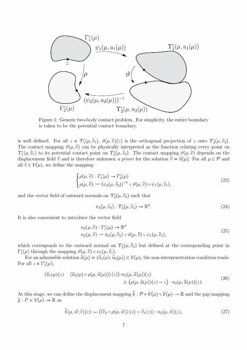
Figure 1: Generic two-body contact problem. For simplicity, the entire boundaryis taken to be the potential contact boundary.

is well defined. For all z P Υc1pµ, rv1q, ϑpµ, rvqpzq is the orthogonal projection of z onto Υc

2pµ, rv2q.The contact mapping ϑpµ, rvq can be physically interpreted as the function relating every point onΥc

1pµ, rv1q to its potential contact point on Υc2pµ, rv2q. The contact mapping ϑpµ, rvq depends on the

displacement field rv and is therefore unknown a priori for the solution rv rupµq. For all µ P P andall rv P Vpµq, we define the mapping#

ρpµ, rvq : Γc1pµq Ñ Γc2pµq

ρpµ, rvq : pψ2pµ, rv2qq1 ϑpµ, rvq ψ1pµ, rv1q,

(23)

and the vector field of outward normals on Υc2pµ, rv2q such that

n2pµ, rv2q : Υc2pµ, rv2q Ñ Rd. (24)

It is also convenient to introduce the vector field

n2pµ, rvq : Γc1pµq Ñ Rd

n2pµ, rvq : n2pµ, rv2q ϑpµ, rvq ψ1pµ, rv1q,(25)

which corresponds to the outward normal on Υc2pµ, rv2q but defined at the corresponding point in

Γc1pµq through the mapping ϑpµ, rvq ψ1pµ, rv1q.For an admissible solution rupµq pru1pµq, ru2pµqq P Vpµq, the non-interpenetration condition reads:

For all z P Γc1pµq,

pru1pµqpzq pru2pµq ρpµ, rupµqqq pzqq n2pµ, rupµqqpzq¥ρpµ, rupµqqpzq z

n2pµ, rupµqqpzq. (26)

At this stage, we can define the displacement mapping rk : PVpµqVpµq Ñ R and the gap mappingrg : P Vpµq Ñ R as

rkpµ, rw; rvqpzq : pprv2 ρpµ, rwqq pzq rv1pzqq n2pµ, rwqpzq, (27)

7

and rgpµ, rwqpzq : pz ρpµ, rwqpzqq n2pµ, rwqpzq, (28)

for all z P Γc1pµq. The distinction between the arguments rv and rw in (27) is introduced so that rk is

linear with respect to rv. Hence, (26) can be recast as rkpµ, rupµq; rupµqq ¤ rgpµ, rupµqq, leading to theinequality constraint considered in (1). For all µ P P , the admissible displacement rupµq P Vpµq isthen solution to $'&'%

rupµq argminrvPVpµq

1

2rapµ; rv, rvq rfpµ; rvq

rkpµ, rupµq; rupµqq ¤ rgpµ, rupµqq a.e. on Γc1pµq.

(29)

Remark 2 (Geometric interpretation). As proven in [22], Section 3.7.3, the constraint (26) isequivalent to

Ω1pµ, ru1pµqq X Ω2pµ, ru2pµqq Υc1pµ, ru1pµqq XΥc

2pµ, ru2pµqq, (30)

whereΩipµ, ruipµqq : pId ruipµqqpΩipµqq, @i P t1, 2u, (31)

i.e. the intersection of the two deformed solids Ω1pµ, ru1pµqq and Ω2pµ, ru2pµqq is necessarily a subsetof their contact boundaries. Note that the indices 1 and 2 play symmetric roles in (30).

3.3 Reference domain

Let us now detail how the frictionless contact problem introduced in Sections 3.1-3.2 can be recastinto the form (1) using a parameter-independent geometry. We assume that there exists a bi-Lipschitzdiffeomorphism called geometric mapping hpµq defined on a parameter-independent reference domainΩ such that

hpµq : Ω Ñ Ωpµq

x ÞÑI

i1

hipµqpxq1Ωipxq,

(32)

where tΩiuIi1 is a partition of Ω. Using this geometric mapping, we introduce the reference Hilbert

spaceV : H1pΩ;Rdq, (33)

composed of functions defined on Ω such that Vpµq : V hpµq1 : tv hpµq1 | v P Vu. For alli P t1, . . . , Iu, we set

Ωipµq : hipµqpΩiq. (34)

In what follows, we assume for simplicity that I 2, which corresponds to the situation fromSection 3 where there are two disjoint solids Ω1pµq and Ω2pµq that can come into contact. We fixthe contact boundaries Γci , i P t1, 2u, on the parameter-independent configuration Ω, and we definethe parametric contact boundaries Γcipµq, i P t1, 2u, as

Γcipµq : hipµqpΓciq, @i P t1, 2u. (35)

Note that hipµq|Γci

defines a diffeomorphism from Γci to Γcipµq for all i P t1, 2u.

8

Let us now define the forms a : PVV Ñ R, f : PV Ñ R, and the mappings k : PVV Ñ Rand g : P V Ñ R such that, for all µ P P and v, w P V ,

apµ; v, wq : ra µ; v hpµq1, w hpµq1, (36)

fpµ;wq : rf µ;w hpµq1, (37)

kpµ,w; vq : rk µ,w hpµq1; v hpµq1 det

Jacph1pµq|Γc

1q , (38)

gpµ,wq : rg µ,w hpµq1 det

Jacph1pµq|Γc

1q , (39)

where detJacph1pµq|Γc

1pµqq

refers to the determinant of the Jacobian matrix of h1pµq|Γc1pµq

. It is clearthat for all µ P P , finding rupµq P Vpµq solution to (29) is equivalent to finding upµq P V solution to$&%upµq argmin

vPV

1

2apµ; v, vq fpµ; vq

kpµ, upµq;upµqq ¤ gpµ, upµqq a.e. on Γc1,

(40)

via the identity rupµq upµqhpµq1. Problem (40) is of the same form as Problem (1) with Γc : Γc1;moreover, the forms a, f and the mappings k, g satisfy the assumptions described in Section 2. Thedual formulation of (40) is (5) with the Lagrangian defined in (6) on VW withW : L2pΓc;Rq.Note that in the context of contact mechanics, the constraint is expressed using the normals in thedeformed configuration and not on the reference one.

Remark 3 (Use of Jacobian). The factor involving the Jacobian is not needed in (38)-(39) since theconstraint is enforced pointwise in (40). One also sees that the operation of mapping from Ω to Ωpµqcommutes with the devising of the dual formulation. Indeed, letting Wpµq : L2pΓc1pµq;Rq, the

dual formulation on the parameter-dependent domain Ωpµq is to find prupµq, rλpµqq P Vpµq Wpµqsuch that

prupµq, rλpµqq arg minmaxrvPVpµq,rηPWpµq

rLpµqprv, rηq,where the Lagrangian rLpµq : Vpµq Wpµq Ñ R is defined as

rLpµqprv, rηq :1

2rapµ; rv, rvq rfpµ; rvq »

Γc1pµq

rkpµ, rv; rvqrη »Γc1pµq

rgpµ, rvqrη .Then the solutions to the dual formulations posed on Ω and on Ωpµq are linked by the relationsrupµq upµq hpµq1 and rλpµq λpµq h1pµq

1|Γc

1pµq.

4 The reduced-basis model

In this section, we return to the abstract setting of Section 2 and we derive a general RB formulationfor the nonlinear minimization problem (1), and more precisely its algebraic saddle-point formula-tion (9).

4.1 Reduced basis spaces

Recall that VN and WR are the FEM discretizations of the Hilbert space V and the cone W,

respectively. In view of an accurate approximation of the solution manifold, we introduce the primal

9

RB subspace pVN and the dual RB subcone xWR that satisfy

pVN VN V and xWR W

R W, (41)

where the subscripts refer to the dimensions and are typically such that N ! N and R ! R.Let pθnq1¤n¤N be a (orthonormal) basis of pVN and let pξrq1¤r¤R be generating vectors of the conexW

R , i.e., xWR spantξ1, . . . , ξRu. For all µ P P , the primal RB solution pupµq P pVN and the dual

RB solution (Lagrange multipliers) pλpµq P xWR that approximate the HF solution puN pµq, λRpµqq P

VN WR are decomposed as

pupµq N

n1

punpµqθn and pλpµq R

r1

pλrpµqξr, (42)

with real numbers punpµq for all n P t1, . . . , Nu and non-negative real numbers pλrpµq for all r P

t1, . . . , Ru. Introducing the component vectors pupµq : ppunpµqq1¤n¤N and pλpµq : ppλrpµqq1¤r¤R, for

all µ P P , the RB formulation of (9) reads: Find ppupµq, pλpµqq P RN RR such that

ppupµq, pλpµqq P arg minmaxpvPRN ,pηPRR

1

2pvT pApµqpv pvTpfpµq pηT pKpµ, pvqpv pgpµ, pvq, (43)

with the matrices pApµq P RNN and pKpµ, pvq P RRN such that

pApµqpn apµ; θn, θpq, (44a)

pKpµ, pvqrn »Γc

k

µ,

N

i1

pviθi; θnξr, (44b)

and the vectors pfpµq P RN and pgpµ, pvq P RR such that

pfpµqp fpµ; θpq, (45a)

pgpµ, pvqr »Γc

g

µ,

N

i1

pviθi ξr. (45b)

4.2 Separation of the elastic energy

We assume the existence of two integers Ja and Jf and of continuous bilinear forms aj : V V Ñ R,with 1 ¤ j ¤ Ja, and continuous linear forms fj : V Ñ R, with 1 ¤ j ¤ Jf , such that the bilinearform apµ; , q and the linear form fpµ; q can be affinely decomposed as follows: For all v, w P V ,

apµ; v, wq Ja¸j1

αaj pµqajpv, wq, and fpµ;wq Jf¸j1

αfj pµqfjpwq, (46)

for some functions αaj : P Ñ R, for all 1 ¤ j ¤ Ja, and αfj : P Ñ R, for all 1 ¤ j ¤ Jf .The separated representations in (46) hold true in the setting of contact mechanics considered in

Section 3 under some reasonable assumptions. Let us exemplify the case of the load fpµ;wq. For all

10

w P V , using the definition of the geometric mapping hpµq in (32), we have

fpµ;wq

»Ωpµq

`pµq w hpµq1 2

i1

»Ωipµq

`pµq w hipµq1

2

i1

»Ωi

`pµqphipµqpxqq wpxq |det pJacphipµqqpxqq| dx,

(47)

where the notation det pJacphipµqqq refers to the determinant of the Jacobian matrix of the geometricmapping hipµq. Let us assume that the load function `pµq is space-independent and that the geometricmappings hipµq, i P t1, 2u, are affine, i.e. that there exists Mipµq P Rdd and bipµq P Rd such that forall x P Ωi, hipµqpxq Mipµqx bipµq, for all µ P P . These assumptions are satisfied in the numericalcases presented in Section 6. Then, we obtain, for all v P V ,

fpµ;wq 2

i1

»Ωi

`pµq wpxq |detMipµq| dx 2

i1

|detMipµq| `pµq

»Ωi

wpxq dx. (48)

Let pekq1¤k¤d be the canonical basis of Rd, and let `kpµq : ek `pµq for all 1 ¤ k ¤ d. Consequently,in (46), we have Jf 2d, and for all 1 ¤ j ¤ 2d, αfj pµq : hipµq`kpµq and fjpwq :

³Ωiek wpxq dx,

where k : tpj 1q2u 1 and i : j 2pk 1q (the notation tu standing for the integer part).Similarly, under the same assumption on hpµq, a separated representation of apµ; , q is available.

In the general case where the dependencies on µ are non-affine, one typically resorts to theEIM [16, 17] in order to build approximate separated representations of apµ; , q and fpµ; q.

The separated expressions (46) imply that the matrix pApµq defined in (44a) and the vector pfpµqdefined in (45a) can be affinely decomposed under the form

pApµqnp

Ja¸j1

αaj pµqpAj,np and

pfpµqp

Jf¸j1

αfj pµqpfj,p, @1 ¤ n, p ¤ N, (49)

where pAj,np : ajpθp, θnq and pfj,p : fjpθpq. The key point is that the dependencies on µ and n, p are

separated in (49). Therefore, the matrix pAj,np and the vector pfj,p are offline-computable, and all that

remains to be performed during the online stage is the assembly of the matrix pApµq and the vectorpfpµq using (49) for each new parameter value µ P P .

4.3 Separation of the constraint

The remaining bottleneck is the computation of the matrix pKpµ, pvq and the vector pgpµ, pvq in (44b)and (45b) respectively. Indeed, these computations require parameter-dependent reconstructionsusing the FEM basis functions pθnq1¤n¤N in order to compute the integrals over Γc. The key idea isto search for approximations κMk and γMg of the nonlinear mappings κ : P t1, . . . ,N u Γc Ñ Rand γ : P Γc Ñ R defined such that

κpµ, n, xq : kpµ, upµq;φnqpxq and γpµ, xq : gpµ, upµqqpxq. (50)

Our goal in building these approximations is to separate the dependence on µ from the dependenceon the other variables. More precisely, for some integers Mk,M g ¥ 1, we look for (accurate) ap-proximations κMk : P t1, . . . ,N u Γc Ñ R of κ and γMg : P Γc Ñ R of γ in the separated

11

form

κMkpµ, n, xq :Mk¸j1

ϕκj pµqqκj pn, xq, γMgpµ, xq :

Mg¸j1

ϕγj pµqqγj pxq, (51)

where Mk (resp. M g) is called the rank of the approximation and ϕκj (resp. ϕγj ) are real-valuedfunctions of the parameter µ that are found by interpolation. For κMk , we interpolate over a setof Mk pairs tpnκ1 , x

κ1q, . . . , pn

κMk , x

κMkqu in t1, . . . ,N u Γc, whereas for γMg , we interpolate over a

set of M g points txγ1 , . . . , xγMgu in Γc. The interpolation is performed using the EIM [16] and leads

to the vector pκpµ, pvq P RMk, the matrix Bκ P RMkMk

, the vector pγpµ, pvq P RMgand the matrix

Bγ P RMgMgdefined as follows: $'''&'''%

pκpµ, pvqi : kpµ, pv;φκniqpxκi q,

Bκij qκj pn

κi , x

κi q,pγpµ, pvqi : gpµ, pvqpxγi q,

Bγij qγj px

γi q.

(52)

Note that the EIM guarantees the invertibility of the matrices Bκ and Bγ. After the approximationresulting from the separation of the constraint, the problem (43) becomes (we keep the same notationfor its solution)

ppupµq, pλpµqq P arg minmaxpvPRN ,pηPRR

!1

2pvT pApµqpv pvTpfpµq pηT Dκpµ, pvqpv Dγppvqpγpµ, pvq), (53)

with the matrices

Dκpµ, pvq :Mk¸j1

Cκj ppB

κq1pκpµ; pvqqj and Dγ : CγpBγq1, (54)

where Cκj P RRN and Cγ P RRMg

are given by

Cκj :

N

i1

»Γc

θn,iqκj pi, qξr

rn

and Cγ :

»Γc

qγj1ξr

pj1, (55)

for all j P t1, . . . ,Mκu, all r P t1, . . . , Ru, all n P t1, . . . , Nu, and all j1 P t1, . . . ,Mγu.The overall computational procedure can now be split into two stages:

(i) An offline stage where one precomputes on the one hand the RB subspace pVN and the RB

subcone xWR leading to the vectors tpfru1¤r¤Jf in RN and the matrices tpAru1¤r¤Ja in RNN ,

and on the other hand the EIM pairs tpnκi , xκi qu1¤i¤Mk , the EIM points txγi u1¤i¤Mg , the EIM

functions tqκj u1¤j¤Mk , and the EIM functions tqγj u1¤j¤Mg , leading to the matrices Bκ P RMkMk,

Bγ P RMgMg, tCκ

j u1¤j¤Mk RRN , and Cγ P RRMg. The offline stage is discussed in more

detail in Section 5.

(ii) An online stage to be performed each time one wishes to compute a new solution for a parameter

µ P P . All that remains to be performed is to assemble the vector pfpµq P RN and the matrixpApµq P RNN using (49), to compute the vectors pκpµ, pvq P RMkand pγpµ, pvq P RMg

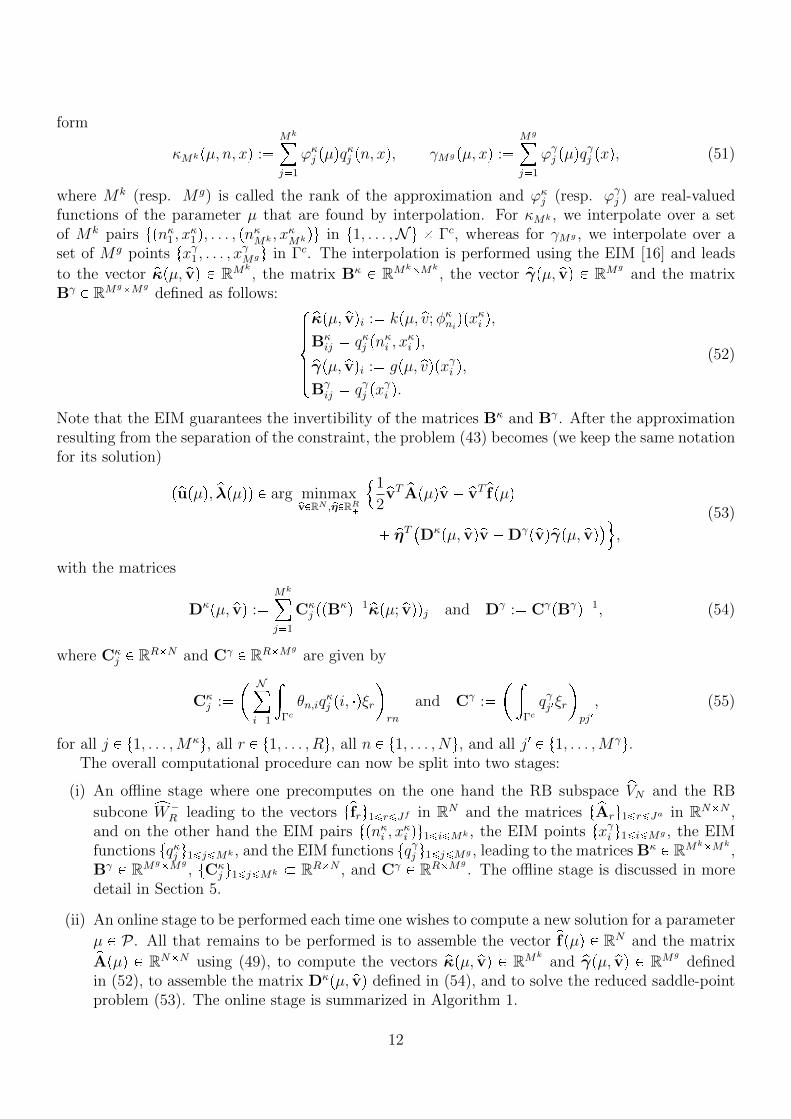
definedin (52), to assemble the matrix Dκpµ, pvq defined in (54), and to solve the reduced saddle-pointproblem (53). The online stage is summarized in Algorithm 1.

12

Algorithm 1 Online stage

Input : µ, tpfju1¤j¤Jf , tpAju1¤j¤Ja , tpnκi , xκi qu1¤i¤Mk , txγi u1¤i¤Mg , tqκj u1¤j¤Mk , tqγj u1¤j¤Mg , Bκ,

tCκj u1¤j¤Mk and Dγ.

1: Assemble the vector pfpµq and the matrix pApµq using (49)2: Compute pκpµ, pvq and pγpµ, pvq using (52)3: Compute Dκpµq using pκpµ, pvq and (54)

4: Solve the reduced saddle-point problem (53) to obtain pupµq and pλpµqOutput : pupµq and pλpµq

Remark 4 (EIM matrices). The computations in Algorithm 1 only require the knowledge of thematrix pBκq1. In order to optimize the computational costs, Bκ is inverted during the offline stage.The matrix Bγ is also inverted when computing the matrix Dγ during the offline stage (see (54)).Since these matrices may be ill-conditioned, whenever an inversion is required, a linear system solveis recommended, along with the storage of the LU decomposition to be used whenever a vector multi-plication by the EIM matrix is needed during the online stage.

Remark 5 (EIMs on k and g). Owing to the quasi-linear structure of the inequality constraint, thereduced problem (53) can be solved using the Kacanov method. At first glance, the influence of thissolution choice is that we have to perform the EIM twice since the mappings k and g are separated oneat a time. Were we to use a Newton method by considering the one-term constraint ζpµ, upµqq ¤ 0(see (2)), we would only perform a single EIM. However, an additional EIM would be needed inthe Newton method in order to compute the Jacobian preconditioning matrix. Thus, both methods(Kacanov or Newton) lead to two distinct EIMs and the storage cost is essentially the same.

5 The offline stage

There are two main tasks to be performed during the offline stage:

(T1) Build the rank-Mk and the rank-M g EIM approximations in (51);

(T2) Explore the solution manifold in order to construct the linear subspace pVN VN of dimension

N and the subcone xWR W

R of dimension R.

Tasks (T1) and (T2) can be performed independently and in whatever order. Since Task (T1) canbe considered to be standard, we only discuss Task (T2), i.e., the construction of the sets of primaland dual RB functions with cardinalities N and R respectively. First, as usual in RB methods, thesolution manifold is explored by considering a training set for the parameter values. For simplicity,one can consider the same training set Ptr as for the EIM approximations. This way, one onlyexplores the collection of snapshots Spri tupµquµPPtr and Sdu tλpµquµPPtr in the primal and dualsolution manifolds respectively. For this exploration to be informative, the training set Ptr has tobe chosen large enough. In the present setting where HF solutions are to be computed for all theparameters in Ptr when constructing the EIM approximations, the present choice is to compressthese computations by means of a Proper Orthogonal Decomposition (POD) [23, 24, 25] to define

the primal RB subspace pVN . One can also resort to the strong greedy algorithm using the true

13

projection error. Choosing between the POD and the strong greedy depends on whether one aimsat an L2-error or H1-error (POD) or an L8-error (strong greedy) over the parameter domain.

Bearing in mind that the dual RB cone xWR is meant to represent the set of Lagrange multipliers,

its spanning vectors should all have non-negative components. Consequently, the POD is not appro-priate to build xW

R . If the training set has a moderate size, one could keep all the Lagrange multipliersnapshots, especially if they have been computed via a posteriori error estimation. In [4], it is sug-gested to use the Non-negative Matrix Factorization (NMF) algorithm [5] whenever the number oftraining snapshots is relatively large, for instance in the case of a time-dependent problem. For a setof snapshots Sdu and an integer R, the procedure NMFpSdu, Rq returns R vectors pw1, . . . , wRq withnon-negative components (the procedure is briefly recalled in Section A). ////////////////Nonetheless,/////the////////////resulting/////dual//////RB//////cone//////can////be/////less///////////accurate///////than/////the/////////primal//////RB////////space. Moreover, the user does not specifyan error tolerance but only the cardinality of the family of vectors generating the dual RB cone. Inpractice, it is often difficult to anticipate how well the dual RB cone approximates the HF cone onlyfrom its cardinality (see the numerical results in Section 6 for illustrations).

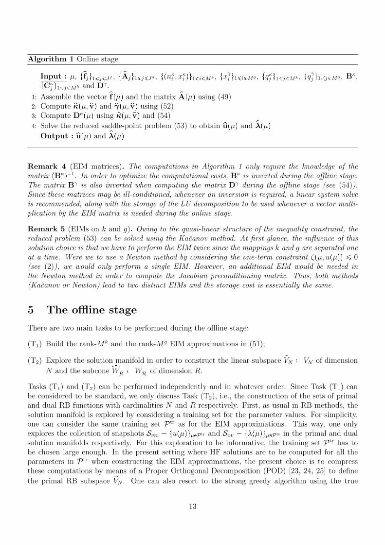
Here, we suggest to build a dual hierarchical RB cone from the Lagrange multiplier snapshotscomputed offline by means of a so-called the Cone-Projected Greedy (CPG) algorithm. In the spiritof weak greedy algorithms, the idea is to order the snapshots depending on their relevance to representthe entire set of snapshots. The algorithm reads as follows: First, we choose µ1 P Ptr such that

µ1 P argmaxµPPtr

λpµqΛ. (56)

The most natural choice for the norm on the Lagrange multipliers is Λ L2pΓcq. However, atthe discrete level, one can also consider the choice Λ `8pΓc,trq, where Γc,tr Γc is a discretesubset of Γc.

Afterwards, at each iteration n ¥ 2, we define the convex cone pKn1 spantλpµ1q, . . . , λpµn1qu

and select a new parameter value µn P Ptr using the criterion

µn P argmaxµPPtr

λpµq ΠpK

n1pλpµqqΛ, (57)

where ΠpK

n1is the L2-orthogonal projector onto the convex cone pK

n1. At each iteration, we check

whether or not the stopping criterion

maxµPPtr

λpµq ΠpK

n1pλpµqqΛ ¤ εdu, (58)

is fulfilled. One can also consider a relative error criterion instead of an absolute one by dividingthe left-hand side of (58) by λpµqΛ. The CPG algorithm is summarized in Algorithm 2. Themain difference between the CPG and the angle-greedy algorithm from [13] is that the latter selectsthe parameter that maximizes the error of a linear projection. In other words, in the angle-greedyalgorithm, line 5 of Algorithm 2 is replaced by µn P argmaxµPPtr λpµq Π

xWn1pλpµqqΛ, wherexWn1 spantλ1pµq, . . . , λn1pµqu is a linear space. Hence, the stopping criterion in the angle-greedy

algorithm does not necessarily reflect the accuracy obtained for the training set, whereas the stoppingcriterion for the CPG represents an accuracy that is effectively satisfied for the training set whenapproximating its elements by positive projections on the RB dual cone. Differences between thetwo algorithms are expected to appear when some Lagrange multipliers are (or are close to being)collinear. An elementary illustration is presented in Remark 6. However, in practice, the angle-greedy algorithm turns out to be efficient for the test cases considered in [13], and it is also the

14

case for the test cases considered herein. When it comes to computational cost, the angle-greedyalgorithm is somewhat faster than the CPG algorithm since the former performs linear projectionswhereas the latter requires positive projections. The availability of an efficient, off-the-shelf libraryto perform positive projections (see [26]) is a further motivation for using the CPG. For instance, forthe test case discussed in Section 6.3 below, the execution time of the CPG is about ten times thatof the angle-greedy algorithm, but it represents less than 1% of the total cost, the constrained HFcomputations being the most expensive part of the offline stage.

Remark 6 (Comparison in a simplified setting). Consider an angle ζ P s0, π6s and the training setof Lagrange multipliers L te1, e2, e3, e4u composed of the following column vectors in R3:

e1

cospζqsinpζq

0

, e2 2

cosp2ζqsinp2ζq

0

, e3 3

2

cosp3ζqsinp3ζq

0

, e4

cosp2ζqsinp2ζqsinpζ2q

. (59)

Consider the cone pK2 spante2, e3u. Then the CPG selects e1 as the next vector since it is the

most distant to the cone, whereas the angle-greedy criterion selects e4 which is the most distant to theplane spante2, e3u. The difference in the selection between the CPG and the angle-greedy algorithmshas been triggered here by the fact that e1 is in spante2, e3u.

Algorithm 2 Cone-Projected Greedy (CPG) algorithm

Input : Ptr and εdu ¡ 01: Compute Sdu : tλpµquµPPtr # HF solutions

2: Set pK0 : t0u

3: Set n : 1 and r1 : 2εdu4: while (rn ¡ εdu) do5: Search µn P argmax

µPPtr

λpµq ΠpK

n1pλpµqqΛ

6: Set pKn : spantλpµ1q, . . . , λpµnqu

7: Set n : n 18: Set rn : max

µPPtrλpµq Π

pK

n1pλpµqqΛ

9: end while10: Set R : n 1

Output : xWR : pK

R .

Remark 7 (Elementary compression). Additional computational savings can be achieved by sup-pressing the constraints that are never saturated for any of the parameters in the training set Ptr

but were initially introduced in the HF model. In practice, one can reduce the dimensions of thematrix Kpµ,upµqq and the vector gpµ,upµqq appearing in (9) by removing the lines and columns ofKpµ,upµqq and the components of gpµ,upµqq that always vanish no matter the value of the parameterµ P Ptr.

6 Numerical results

In this section, we illustrate the above developments by two numerical examples related to elasticfrictionless contact in a two-dimensional framework. The goal is to illustrate the computational

15

performance of the proposed method. We first present two different methodologies to address thediscretization of the constraint. Hence, Section 6.1 does not deal with model reduction and thereader familiar with the material can skip it. The first example is the contact problem between twohalf-disks introduced by Hertz in [18], whereas the second investigates a contact problem between aring and a block as described in [19]. The HF computations use a combination of Freefem++ [27]and Python, whereas the reduced-order modeling algorithms have been developed in Python usingthe convex optimization package cvxopt [26].

6.1 Discretization of the HF problem

Continuous piecewise affine finite elements are used to discretize the displacement field on trian-gular meshes of Ω1 and Ω2. We consider two different strategies for discretizing the constraint inthe HF saddle-point problem (9); namely, a collocation method and the so-called Local AverageContact method (LAC) introduced in [28]. The collocation method amounts to node-to-segmentnon-interpenetration constraints in 2D (or to the equivalent node-to-face constraints in 3D). How-ever, in many contexts, this method can produce dual solutions with oscillations thereby degradingthe accuracy of the computations. The LAC method was designed to overcome the oscillation phe-nomenon. The price to pay is that the constraint is expressed in a somewhat less local form.

6.1.1 The collocation method

The collocation method expresses the non-interpenetration constraints at given collocation nodes.We choose these nodes, say tzru1¤r¤R, to be the boundary vertices of the mesh from Ω1 located onΓc Γc1 (other choices are possible). Thus, the non-interpenetration constraints read

kpµ, uN pµq;uN pµqqpzrq ¤ gpµ, uN pµqqpzrq, @r P t1, . . . ,Ru. (60)

The conditions in (60) can be interpreted as»Γc

kpµ, uN pµq;uN pµqqψr ¤

»Γc

gpµ, uN pµqqψr, @r P t1, . . . ,Ru, (61)

where tψru1¤r¤R are P0 basis functions with support centered on the collocation nodes, provided aone-node quadrature at the collocation nodes is used to approximate the integrals in (61).

6.1.2 The LAC method

In the LAC method, the admissible displacements satisfy the average non-interpenetration conditions»Γc

kpµ, uN pµq;uN pµqqψr ¤

»Γc

gpµ, uN pµqqψr, @r P t1, . . . ,Ru, (62)

where tψru1¤r¤R are P0 basis functions defined on Γc and supported on non-overlapping macro-segments Ir Γc. The sole requirement on the macro-segments Ir is that each one contains at leastone internal degree of freedom for the displacement. For instance, for a polynomial degree k 1 ofthe primal HF space, the macro-segments comprise two adjacent segments that are boundary sideson Γc of the mesh from Ω1. In other words, on a fixed mesh, there are two times more basis functionsto enforce the constraints in the collocation method than in the LAC method. The integrals in (62)are approximated using Simpson’s rule on Ir. Since the midpoint of a macro-segment Ir is also aboundary vertex of the mesh from Ω1, this means that the integrals in (62) are evaluated only atthese boundary vertices.

16

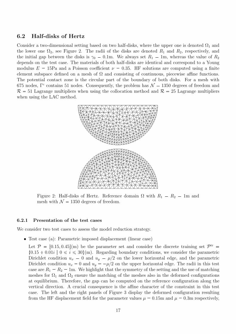
6.2 Half-disks of Hertz

Consider a two-dimensional setting based on two half-disks, where the upper one is denoted Ω1 andthe lower one Ω2, see Figure 2. The radii of the disks are denoted R1 and R2, respectively, andthe initial gap between the disks is γ0 0.1m. We always set R1 1m, whereas the value of R2

depends on the test case. The materials of both half-disks are identical and correspond to a Youngmodulus E 15Pa and a Poisson coefficient ν 0.35. HF solutions are computed using a finiteelement subspace defined on a mesh of Ω and consisting of continuous, piecewise affine functions.The potential contact zone is the circular part of the boundary of both disks. For a mesh with675 nodes, Γc contains 51 nodes. Consequently, the problem has N 1350 degrees of freedom andR 51 Lagrange multipliers when using the collocation method and R 25 Lagrange multiplierswhen using the LAC method.

Figure 2: Half-disks of Hertz. Reference domain Ω with R1 R2 1m andmesh with N 1350 degrees of freedom.

6.2.1 Presentation of the test cases

We consider two test cases to assess the model reduction strategy.

• Test case (a): Parametric imposed displacement (linear case)

Let P r0.15, 0.45s(m) be the parameter set and consider the discrete training set Ptr t0.15 0.01i | 0 ¤ i ¤ 30u(m). Regarding boundary conditions, we consider the parametricDirichlet condition ux 0 and uy µ2 on the lower horizontal edge, and the parametricDirichlet condition ux 0 and uy µ2 on the upper horizontal edge. The radii in this testcase are R1 R2 1m. We highlight that the symmetry of the setting and the use of matchingmeshes for Ω1 and Ω2 ensure the matching of the meshes also in the deformed configurationsat equilibrium. Therefore, the gap can be computed on the reference configuration along thevertical direction. A crucial consequence is the affine character of the constraint in this testcase. The left and the right panels of Figure 3 display the deformed configuration resultingfrom the HF displacement field for the parameter values µ 0.15m and µ 0.3m respectively,

17

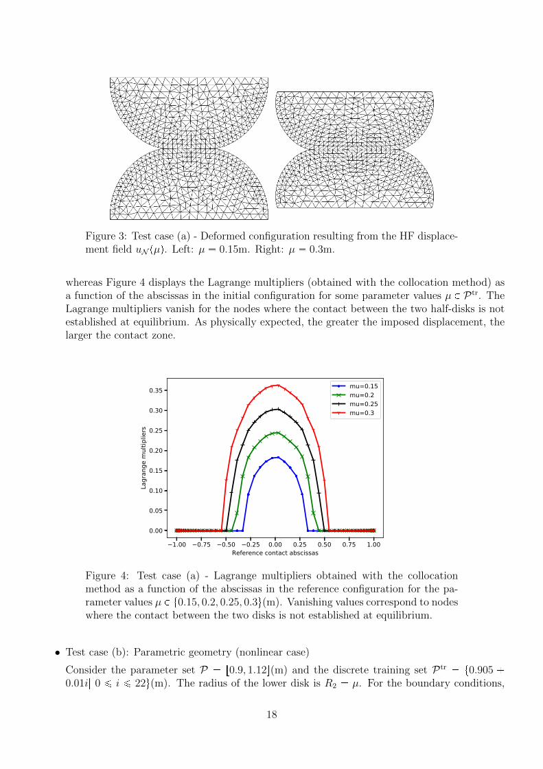
Figure 3: Test case (a) - Deformed configuration resulting from the HF displace-ment field uN pµq. Left: µ 0.15m. Right: µ 0.3m.

whereas Figure 4 displays the Lagrange multipliers (obtained with the collocation method) asa function of the abscissas in the initial configuration for some parameter values µ P Ptr. TheLagrange multipliers vanish for the nodes where the contact between the two half-disks is notestablished at equilibrium. As physically expected, the greater the imposed displacement, thelarger the contact zone.

1.00 0.75 0.50 0.25 0.00 0.25 0.50 0.75 1.00Reference contact abscissas

0.00

0.05

0.10

0.15

0.20

0.25

0.30

0.35

Lagr

ange

mul

tiplie

rs

mu=0.15mu=0.2mu=0.25mu=0.3

Figure 4: Test case (a) - Lagrange multipliers obtained with the collocationmethod as a function of the abscissas in the reference configuration for the pa-rameter values µ P t0.15, 0.2, 0.25, 0.3u(m). Vanishing values correspond to nodeswhere the contact between the two disks is not established at equilibrium.

• Test case (b): Parametric geometry (nonlinear case)

Consider the parameter set P r0.9, 1.12s(m) and the discrete training set Ptr t0.905 0.01i| 0 ¤ i ¤ 22u(m). The radius of the lower disk is R2 µ. For the boundary conditions,

18

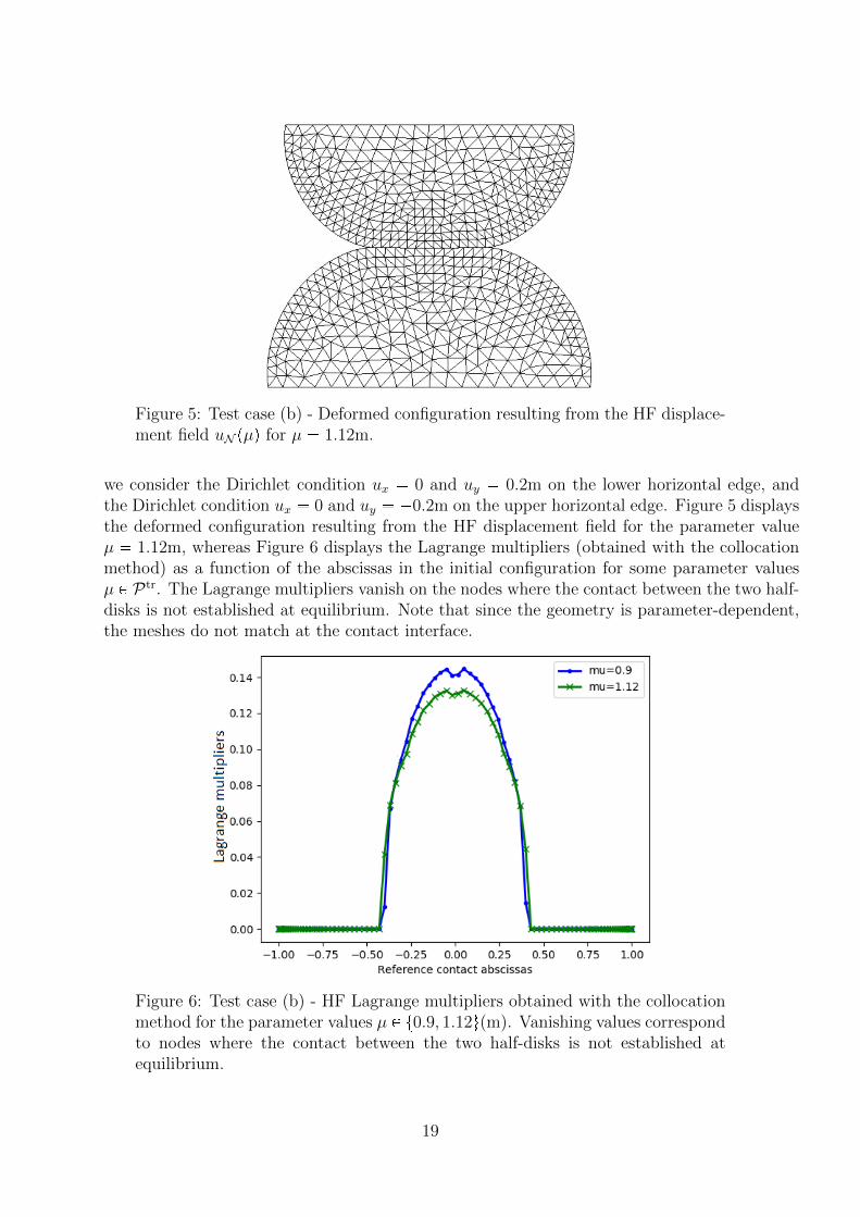
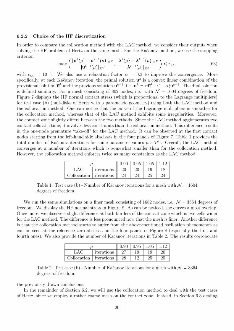
Figure 5: Test case (b) - Deformed configuration resulting from the HF displace-ment field uN pµq for µ 1.12m.

we consider the Dirichlet condition ux 0 and uy 0.2m on the lower horizontal edge, andthe Dirichlet condition ux 0 and uy 0.2m on the upper horizontal edge. Figure 5 displaysthe deformed configuration resulting from the HF displacement field for the parameter valueµ 1.12m, whereas Figure 6 displays the Lagrange multipliers (obtained with the collocationmethod) as a function of the abscissas in the initial configuration for some parameter valuesµ P Ptr. The Lagrange multipliers vanish on the nodes where the contact between the two half-disks is not established at equilibrium. Note that since the geometry is parameter-dependent,the meshes do not match at the contact interface.

Figure 6: Test case (b) - HF Lagrange multipliers obtained with the collocationmethod for the parameter values µ P t0.9, 1.12u(m). Vanishing values correspondto nodes where the contact between the two half-disks is not established atequilibrium.

19

6.2.2 Choice of the HF discretization

In order to compare the collocation method with the LAC method, we consider their outputs whensolving the HF problem of Hertz on the same mesh. For the Kacanov method, we use the stoppingcriterion

max

ukpµq uk1pµqRN

uk1pµqRN,λkpµq λk1pµqRR

λk1pµqRR

¤ εka, (63)

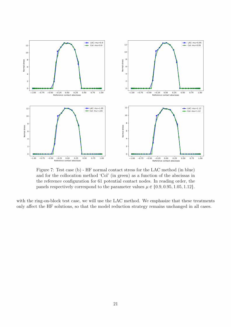
with εka 103. We also use a relaxation factor α 0.3 to improve the convergence. Morespecifically, at each Kacanov iteration, the primal solution uk is a convex linear combination of theprovisional solution uk and the previous solution uk1, i.e. uk αukp1αquk1. The dual solutionis defined similarly. For a mesh consisting of 802 nodes, i.e. with N 1604 degrees of freedom,Figure 7 displays the HF normal contact stress (which is proportional to the Lagrange multipliers)for test case (b) (half-disks of Hertz with a parametric geometry) using both the LAC method andthe collocation method. One can notice that the curve of the Lagrange multipliers is smoother forthe collocation method, whereas that of the LAC method exhibits some irregularities. Moreover,the contact zone slightly differs between the two methods. Since the LAC method agglomerates twocontact cells at a time, it involves less constraints than the collocation method. This difference resultsin the one-node premature ‘take-off’ for the LAC method. It can be observed at the first contactnodes starting from the left-hand side abscissas in the four panels of Figure 7. Table 1 provides thetotal number of Kacanov iterations for some parameter values µ P Ptr. Overall, the LAC methodconverges at a number of iterations which is somewhat smaller than for the collocation method.However, the collocation method enforces twice as many constraints as the LAC method.

µ 0.90 0.95 1.05 1.12LAC iterations 20 20 19 18

Collocation iterations 24 24 25 24

Table 1: Test case (b) - Number of Kacanov iterations for a mesh with N 1604degrees of freedom.

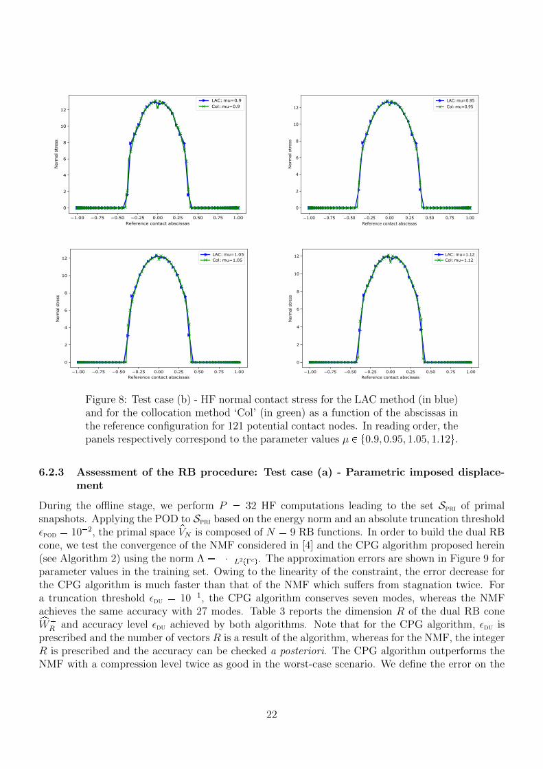
We run the same simulations on a finer mesh consisting of 1682 nodes, i.e., N 3364 degrees offreedom. We display the HF normal stress in Figure 8. As can be noticed, the curves almost overlap.Once more, we observe a slight difference at both borders of the contact zone which is two cells widerfor the LAC method. The difference is less pronounced now that the mesh is finer. Another differenceis that the collocation method starts to suffer from the above-mentioned oscillation phenomenon ascan be seen at the reference zero abscissa on the four panels of Figure 8 (especially the first andfourth ones). We also provide the number of Kacanov iterations in Table 2. The results corroborate

µ 0.90 0.95 1.05 1.12LAC iterations 27 19 19 20

Collocation iterations 28 12 25 25

Table 2: Test case (b) - Number of Kacanov iterations for a mesh with N 3364degrees of freedom.

the previously drawn conclusions.In the remainder of Section 6.2, we will use the collocation method to deal with the test cases

of Hertz, since we employ a rather coarse mesh on the contact zone. Instead, in Section 6.3 dealing

20

1.00 0.75 0.50 0.25 0.00 0.25 0.50 0.75 1.00Reference contact abscissas

0

2

4

6

8

10

12

Nor

mal

str

ess

LAC: mu=0.9Col: mu=0.9

1.00 0.75 0.50 0.25 0.00 0.25 0.50 0.75 1.00Reference contact abscissas

0

2

4

6

8

10

12

Nor

mal

str

ess

LAC: mu=0.95Col: mu=0.95

1.00 0.75 0.50 0.25 0.00 0.25 0.50 0.75 1.00Reference contact abscissas

0

2

4

6

8

10

12

Nor

mal

str

ess

LAC: mu=1.05Col: mu=1.05

1.00 0.75 0.50 0.25 0.00 0.25 0.50 0.75 1.00Reference contact abscissas

0

2

4

6

8

10

12

Nor

mal

str

ess

LAC: mu=1.12Col: mu=1.12

Figure 7: Test case (b) - HF normal contact stress for the LAC method (in blue)and for the collocation method ‘Col’ (in green) as a function of the abscissas inthe reference configuration for 61 potential contact nodes. In reading order, thepanels respectively correspond to the parameter values µ P t0.9, 0.95, 1.05, 1.12u.

with the ring-on-block test case, we will use the LAC method. We emphasize that these treatmentsonly affect the HF solutions, so that the model reduction strategy remains unchanged in all cases.

21

1.00 0.75 0.50 0.25 0.00 0.25 0.50 0.75 1.00Reference contact abscissas

0

2

4

6

8

10

12

Nor

mal

str

ess

LAC: mu=0.9Col: mu=0.9

1.00 0.75 0.50 0.25 0.00 0.25 0.50 0.75 1.00Reference contact abscissas

0

2

4

6

8

10

12

Norm

al st

ress

LAC: mu=0.95Col: mu=0.95

1.00 0.75 0.50 0.25 0.00 0.25 0.50 0.75 1.00Reference contact abscissas

0

2

4

6

8

10

12

Nor

mal

str

ess

LAC: mu=1.05Col: mu=1.05

1.00 0.75 0.50 0.25 0.00 0.25 0.50 0.75 1.00Reference contact abscissas

0

2

4

6

8

10

12

Nor

mal

str

ess

LAC: mu=1.12Col: mu=1.12

Figure 8: Test case (b) - HF normal contact stress for the LAC method (in blue)and for the collocation method ‘Col’ (in green) as a function of the abscissas inthe reference configuration for 121 potential contact nodes. In reading order, thepanels respectively correspond to the parameter values µ P t0.9, 0.95, 1.05, 1.12u.

6.2.3 Assessment of the RB procedure: Test case (a) - Parametric imposed displace-ment

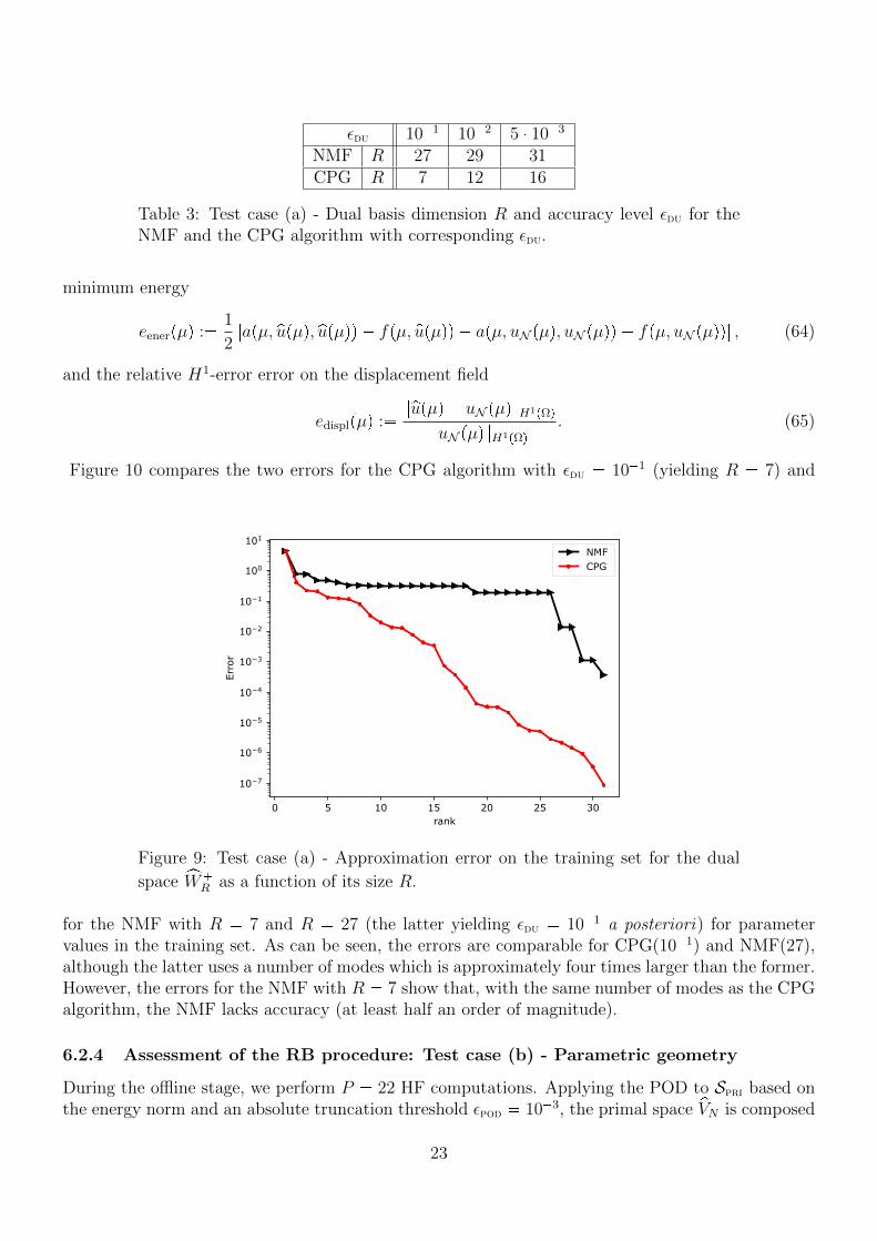
During the offline stage, we perform P 32 HF computations leading to the set Spri of primalsnapshots. Applying the POD to Spri based on the energy norm and an absolute truncation thresholdεpod 102, the primal space pVN is composed of N 9 RB functions. In order to build the dual RBcone, we test the convergence of the NMF considered in [4] and the CPG algorithm proposed herein(see Algorithm 2) using the norm Λ L2pΓcq. The approximation errors are shown in Figure 9 forparameter values in the training set. Owing to the linearity of the constraint, the error decrease forthe CPG algorithm is much faster than that of the NMF which suffers from stagnation twice. Fora truncation threshold εdu 101, the CPG algorithm conserves seven modes, whereas the NMFachieves the same accuracy with 27 modes. Table 3 reports the dimension R of the dual RB conexWR and accuracy level εdu achieved by both algorithms. Note that for the CPG algorithm, εdu is

prescribed and the number of vectors R is a result of the algorithm, whereas for the NMF, the integerR is prescribed and the accuracy can be checked a posteriori. The CPG algorithm outperforms theNMF with a compression level twice as good in the worst-case scenario. We define the error on the

22

εdu 101 102 5 103

NMF R 27 29 31CPG R 7 12 16

Table 3: Test case (a) - Dual basis dimension R and accuracy level εdu for theNMF and the CPG algorithm with corresponding εdu.

minimum energy

eenerpµq :1

2|apµ, pupµq, pupµqq fpµ, pupµqq apµ, uN pµq, uN pµqq fpµ, uN pµqq| , (64)

and the relative H1-error error on the displacement field

edisplpµq :pupµq uN pµqH1pΩq

uN pµqH1pΩq

. (65)

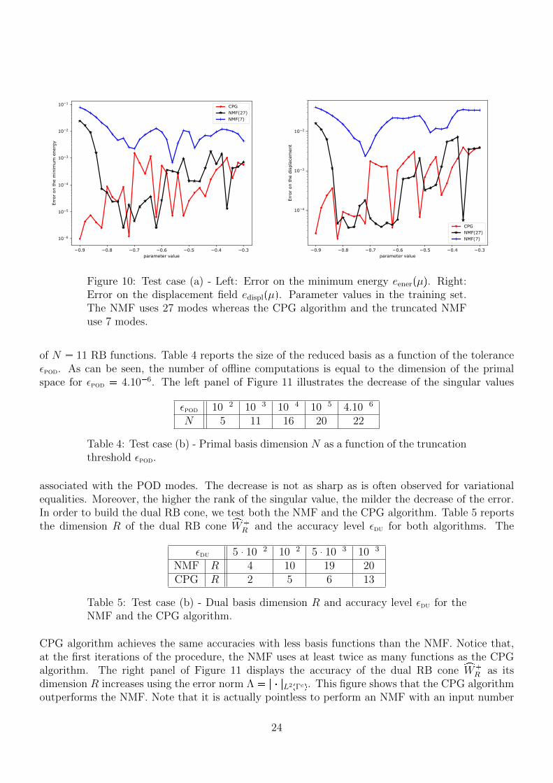
Figure 10 compares the two errors for the CPG algorithm with εdu 101 (yielding R 7) and

0 5 10 15 20 25 30rank

10 7

10 6

10 5

10 4

10 3

10 2

10 1

100

101

Error

NMFCPG

Figure 9: Test case (a) - Approximation error on the training set for the dual

space xWR as a function of its size R.

for the NMF with R 7 and R 27 (the latter yielding εdu 101 a posteriori) for parametervalues in the training set. As can be seen, the errors are comparable for CPG(101) and NMF(27),although the latter uses a number of modes which is approximately four times larger than the former.However, the errors for the NMF with R 7 show that, with the same number of modes as the CPGalgorithm, the NMF lacks accuracy (at least half an order of magnitude).

6.2.4 Assessment of the RB procedure: Test case (b) - Parametric geometry

During the offline stage, we perform P 22 HF computations. Applying the POD to Spri based onthe energy norm and an absolute truncation threshold εpod 103, the primal space pVN is composed

23

0.9 0.8 0.7 0.6 0.5 0.4 0.3parameter value

10 6

10 5

10 4

10 3

10 2

10 1

Err

or

on t

he m

inim

um

energ

y

CPGNMF(27)NMF(7)

0.9 0.8 0.7 0.6 0.5 0.4 0.3parameter value

10 4

10 3

10 2

Err

or

on t

he d

ispla

cem

ent

CPGNMF(27)NMF(7)

Figure 10: Test case (a) - Left: Error on the minimum energy eenerpµq. Right:Error on the displacement field edisplpµq. Parameter values in the training set.The NMF uses 27 modes whereas the CPG algorithm and the truncated NMFuse 7 modes.

of N 11 RB functions. Table 4 reports the size of the reduced basis as a function of the toleranceεpod. As can be seen, the number of offline computations is equal to the dimension of the primalspace for εpod 4.106. The left panel of Figure 11 illustrates the decrease of the singular values

εpod 102 103 104 105 4.106

N 5 11 16 20 22

Table 4: Test case (b) - Primal basis dimension N as a function of the truncationthreshold εpod.

associated with the POD modes. The decrease is not as sharp as is often observed for variationalequalities. Moreover, the higher the rank of the singular value, the milder the decrease of the error.In order to build the dual RB cone, we test both the NMF and the CPG algorithm. Table 5 reportsthe dimension R of the dual RB cone xW

R and the accuracy level εdu for both algorithms. The

εdu 5 102 102 5 103 103

NMF R 4 10 19 20CPG R 2 5 6 13

Table 5: Test case (b) - Dual basis dimension R and accuracy level εdu for theNMF and the CPG algorithm.

CPG algorithm achieves the same accuracies with less basis functions than the NMF. Notice that,at the first iterations of the procedure, the NMF uses at least twice as many functions as the CPGalgorithm. The right panel of Figure 11 displays the accuracy of the dual RB cone xW

R as itsdimension R increases using the error norm Λ L2pΓcq. This figure shows that the CPG algorithmoutperforms the NMF. Note that it is actually pointless to perform an NMF with an input number

24

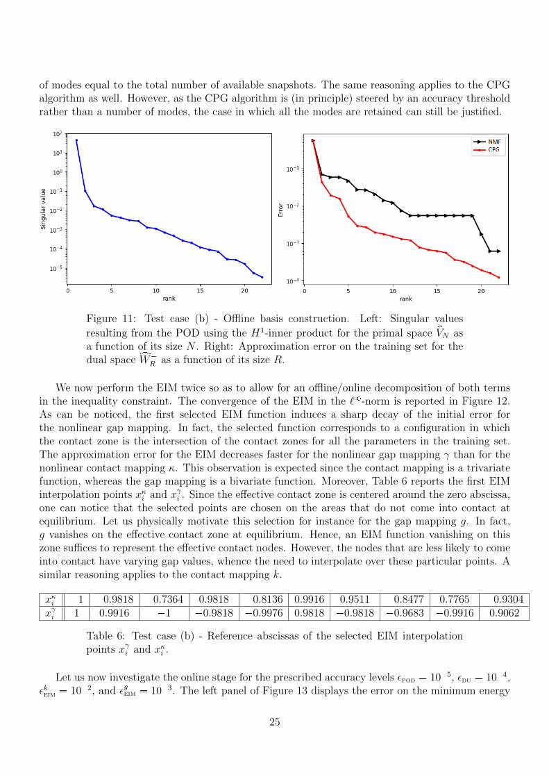
of modes equal to the total number of available snapshots. The same reasoning applies to the CPGalgorithm as well. However, as the CPG algorithm is (in principle) steered by an accuracy thresholdrather than a number of modes, the case in which all the modes are retained can still be justified.

Figure 11: Test case (b) - Offline basis construction. Left: Singular values

resulting from the POD using the H1-inner product for the primal space pVN asa function of its size N . Right: Approximation error on the training set for thedual space xW

R as a function of its size R.

We now perform the EIM twice so as to allow for an offline/online decomposition of both termsin the inequality constraint. The convergence of the EIM in the `8-norm is reported in Figure 12.As can be noticed, the first selected EIM function induces a sharp decay of the initial error forthe nonlinear gap mapping. In fact, the selected function corresponds to a configuration in whichthe contact zone is the intersection of the contact zones for all the parameters in the training set.The approximation error for the EIM decreases faster for the nonlinear gap mapping γ than for thenonlinear contact mapping κ. This observation is expected since the contact mapping is a trivariatefunction, whereas the gap mapping is a bivariate function. Moreover, Table 6 reports the first EIMinterpolation points xκi and xγi . Since the effective contact zone is centered around the zero abscissa,one can notice that the selected points are chosen on the areas that do not come into contact atequilibrium. Let us physically motivate this selection for instance for the gap mapping g. In fact,g vanishes on the effective contact zone at equilibrium. Hence, an EIM function vanishing on thiszone suffices to represent the effective contact nodes. However, the nodes that are less likely to comeinto contact have varying gap values, whence the need to interpolate over these particular points. Asimilar reasoning applies to the contact mapping k.

xκi 1 0.9818 0.7364 0.9818 0.8136 0.9916 0.9511 0.8477 0.7765 0.9304xγi 1 0.9916 1 0.9818 0.9976 0.9818 0.9818 0.9683 0.9916 0.9062

Table 6: Test case (b) - Reference abscissas of the selected EIM interpolationpoints xγi and xκi .

Let us now investigate the online stage for the prescribed accuracy levels εpod 105, εdu 104,εkeim 102, and εgeim 103. The left panel of Figure 13 displays the error on the minimum energy

25

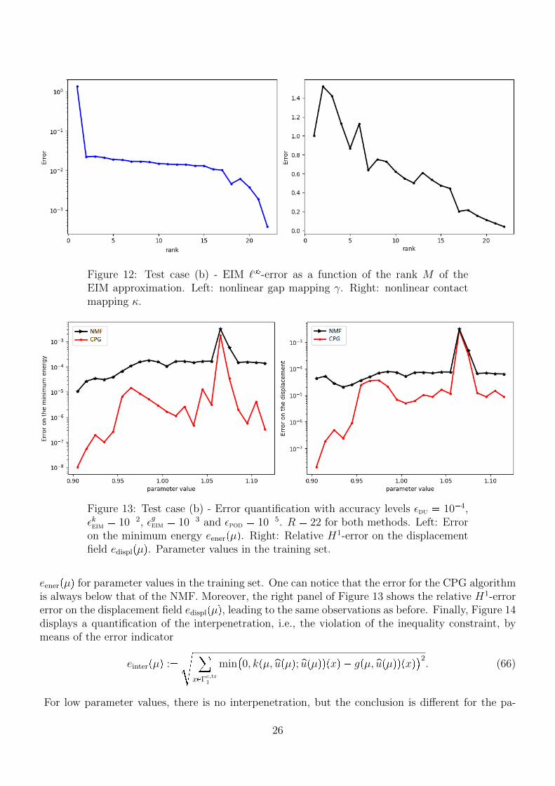
Figure 12: Test case (b) - EIM `8-error as a function of the rank M of theEIM approximation. Left: nonlinear gap mapping γ. Right: nonlinear contactmapping κ.

Figure 13: Test case (b) - Error quantification with accuracy levels εdu 104,εkeim 102, εgeim 103 and εpod 105. R 22 for both methods. Left: Erroron the minimum energy eenerpµq. Right: Relative H1-error on the displacementfield edisplpµq. Parameter values in the training set.

eenerpµq for parameter values in the training set. One can notice that the error for the CPG algorithmis always below that of the NMF. Moreover, the right panel of Figure 13 shows the relative H1-errorerror on the displacement field edisplpµq, leading to the same observations as before. Finally, Figure 14displays a quantification of the interpenetration, i.e., the violation of the inequality constraint, bymeans of the error indicator

einterpµq :

d ¸xPΓc,tr

1

min0, kpµ, pupµq; pupµqqpxq gpµ, pupµqqpxq2

. (66)

For low parameter values, there is no interpenetration, but the conclusion is different for the pa-

26

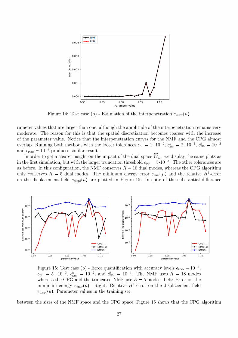
Figure 14: Test case (b) - Estimation of the interpenetration einterpµq.

rameter values that are larger than one, although the amplitude of the interpenetration remains verymoderate. The reason for this is that the spatial discretization becomes coarser with the increaseof the parameter value. Notice that the interpenetration curves for the NMF and the CPG almostoverlap. Running both methods with the looser tolerances εdu 1 102, εkeim 2 101, εgeim 102

and εpod 102 produces similar results.In order to get a clearer insight on the impact of the dual space xW

R , we display the same plots asin the first simulation, but with the larger truncation threshold εdu 5103. The other tolerances areas before. In this configuration, the NMF conserves R 18 dual modes, whereas the CPG algorithmonly conserves R 5 dual modes. The minimum energy error eenerpµq and the relative H1-erroron the displacement field edisplpµq are plotted in Figure 15. In spite of the substantial difference

0.90 0.95 1.00 1.05 1.10parameter value

10 7

10 6

10 5

10 4

10 3

Err

or

on t

he m

inim

um

energ

y

CPGNMF(18)NMF(5)

0.90 0.95 1.00 1.05 1.10parameter value

10 6

10 5

10 4

10 3

Err

or

on t

he d

ispla

cem

ent

CPGNMF(18)NMF(5)

Figure 15: Test case (b) - Error quantification with accuracy levels εpod 104,εdu 5 103, εkeim 102, and εgeim 104. The NMF uses R 18 modeswhereas the CPG and the truncated NMF use R 5 modes. Left: Error on theminimum energy eenerpµq. Right: Relative H1-error on the displacement fieldedisplpµq. Parameter values in the training set.

between the sizes of the NMF space and the CPG space, Figure 15 shows that the CPG algorithm

27

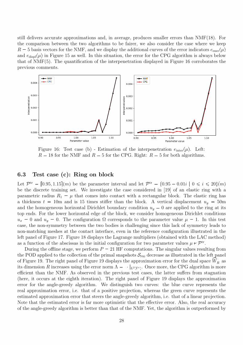
still delivers accurate approximations and, in average, produces smaller errors than NMF(18). Forthe comparison between the two algorithms to be fairer, we also consider the case where we keepR 5 basis vectors for the NMF, and we display the additional curves of the error indicators eenerpµqand edisplpµq in Figure 15 as well. In this situation, the error for the CPG algorithm is always belowthat of NMF(5). The quantification of the interpenetration displayed in Figure 16 corroborates theprevious comments.

Figure 16: Test case (b) - Estimation of the interpenetration einterpµq. Left:R 18 for the NMF and R 5 for the CPG. Right: R 5 for both algorithms.

6.3 Test case (c): Ring on block

Let Ptr r0.95, 1.15spmq be the parameter interval and let Ptr t0.95 0.01i | 0 ¤ i ¤ 20upmqbe the discrete training set. We investigate the case considered in [19] of an elastic ring with aparametric radius R1 µ that comes into contact with a rectangular block. The elastic ring hasa thickness t 10m and is 15 times stiffer than the block. A vertical displacement uy 50mand the homogeneous horizontal Dirichlet boundary condition uy 0 are applied to the ring at itstop ends. For the lower horizontal edge of the block, we consider homogeneous Dirichlet conditionsux 0 and uy 0. The configuration Ω corresponds to the parameter value µ 1. In this testcase, the non-symmetry between the two bodies is challenging since this lack of symmetry leads tonon-matching meshes at the contact interface, even in the reference configuration illustrated in theleft panel of Figure 17. Figure 18 displays the Lagrange multipliers (obtained with the LAC method)as a function of the abscissas in the initial configuration for two parameter values µ P Ptr.

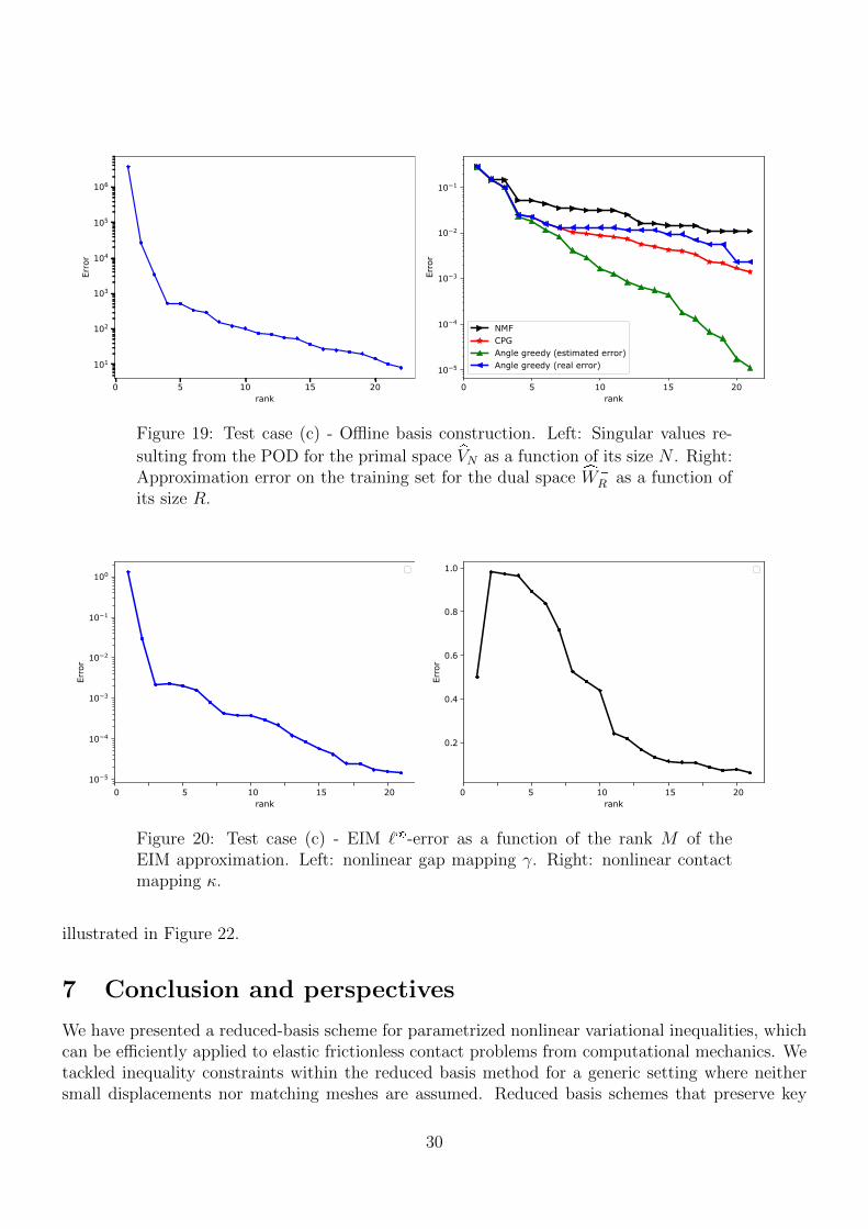
During the offline stage, we perform P 21 HF computations. The singular values resulting fromthe POD applied to the collection of the primal snapshots Spri decrease as illustrated in the left panelof Figure 19. The right panel of Figure 19 displays the approximation error for the dual space xW

R asits dimension R increases using the error norm Λ L2pΓcq. Once more, the CPG algorithm is moreefficient than the NMF. As observed in the previous test cases, the latter suffers from stagnation(here, it occurs at the eighth iteration). The right panel of Figure 19 displays the approximationerror for the angle-greedy algorithm. We distinguish two curves: the blue curve represents thereal approximation error, i.e. that of a positive projection, whereas the green curve represents theestimated approximation error that steers the angle-greedy algorithm, i.e. that of a linear projection.Note that the estimated error is far more optimistic that the effective error. Also, the real accuracyof the angle-greedy algorithm is better than that of the NMF. Yet, the algorithm is outperformed by

28

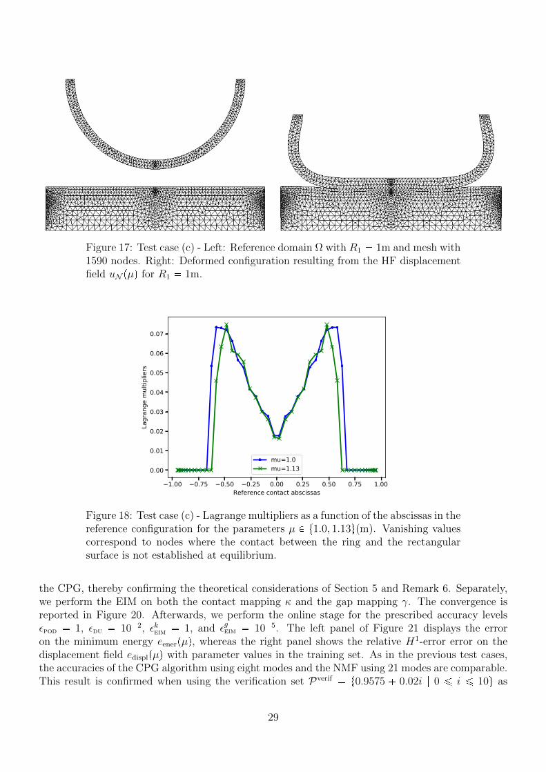
Figure 17: Test case (c) - Left: Reference domain Ω with R1 1m and mesh with1590 nodes. Right: Deformed configuration resulting from the HF displacementfield uN pµq for R1 1m.

1.00 0.75 0.50 0.25 0.00 0.25 0.50 0.75 1.00Reference contact abscissas

0.00

0.01

0.02

0.03

0.04

0.05

0.06

0.07

Lagr

ange

mul

tiplie

rs

mu=1.0mu=1.13

Figure 18: Test case (c) - Lagrange multipliers as a function of the abscissas in thereference configuration for the parameters µ P t1.0, 1.13u(m). Vanishing valuescorrespond to nodes where the contact between the ring and the rectangularsurface is not established at equilibrium.

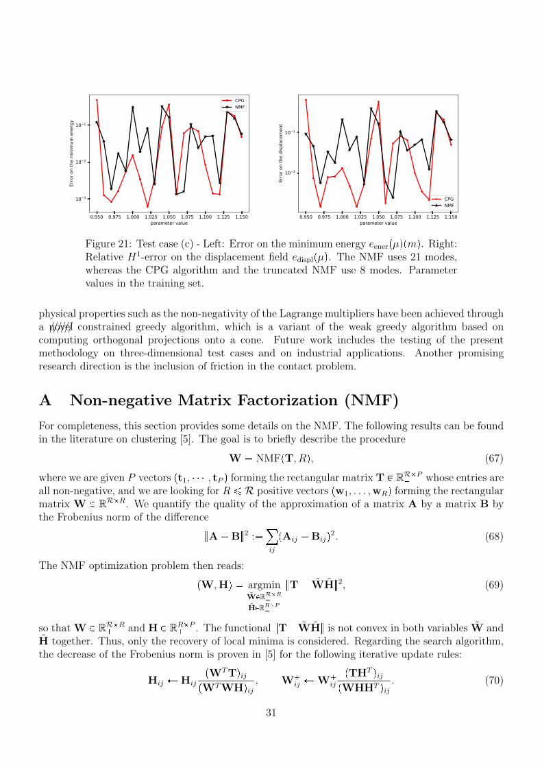
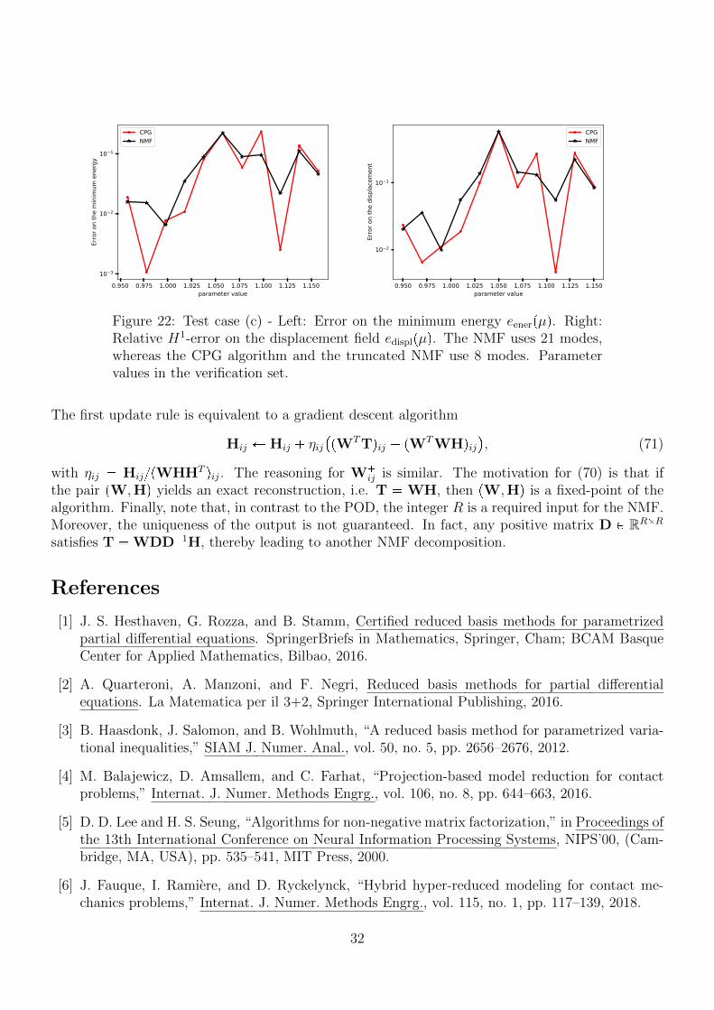
the CPG, thereby confirming the theoretical considerations of Section 5 and Remark 6. Separately,we perform the EIM on both the contact mapping κ and the gap mapping γ. The convergence isreported in Figure 20. Afterwards, we perform the online stage for the prescribed accuracy levelsεpod 1, εdu 102, εkeim 1, and εgeim 105. The left panel of Figure 21 displays the erroron the minimum energy eenerpµq, whereas the right panel shows the relative H1-error error on thedisplacement field edisplpµq with parameter values in the training set. As in the previous test cases,the accuracies of the CPG algorithm using eight modes and the NMF using 21 modes are comparable.This result is confirmed when using the verification set Pverif t0.9575 0.02i | 0 ¤ i ¤ 10u as

29

0 5 10 15 20rank

101

102

103

104

105

106

Erro

r

0 5 10 15 20rank

10 5

10 4

10 3

10 2

10 1

Err

or

NMFCPGAngle greedy (estimated error)Angle greedy (real error)

Figure 19: Test case (c) - Offline basis construction. Left: Singular values re-

sulting from the POD for the primal space pVN as a function of its size N . Right:Approximation error on the training set for the dual space xW

R as a function ofits size R.

0 5 10 15 20rank

10 5

10 4

10 3

10 2

10 1

100

Err

or

0 5 10 15 20rank

0.2

0.4

0.6

0.8

1.0

Err

or

Figure 20: Test case (c) - EIM `8-error as a function of the rank M of theEIM approximation. Left: nonlinear gap mapping γ. Right: nonlinear contactmapping κ.

illustrated in Figure 22.

7 Conclusion and perspectives

We have presented a reduced-basis scheme for parametrized nonlinear variational inequalities, whichcan be efficiently applied to elastic frictionless contact problems from computational mechanics. Wetackled inequality constraints within the reduced basis method for a generic setting where neithersmall displacements nor matching meshes are assumed. Reduced basis schemes that preserve key

30

0.950 0.975 1.000 1.025 1.050 1.075 1.100 1.125 1.150parameter value

10 3

10 2

10 1

Erro

r on

the

min

imum

ene

rgy

CPGNMF

0.950 0.975 1.000 1.025 1.050 1.075 1.100 1.125 1.150parameter value

10 2

10 1

Erro

r on

the

disp

lace

men

t

CPGNMF

Figure 21: Test case (c) - Left: Error on the minimum energy eenerpµqpmq. Right:Relative H1-error on the displacement field edisplpµq. The NMF uses 21 modes,whereas the CPG algorithm and the truncated NMF use 8 modes. Parametervalues in the training set.

physical properties such as the non-negativity of the Lagrange multipliers have been achieved througha //////novel constrained greedy algorithm, which is a variant of the weak greedy algorithm based oncomputing orthogonal projections onto a cone. Future work includes the testing of the presentmethodology on three-dimensional test cases and on industrial applications. Another promisingresearch direction is the inclusion of friction in the contact problem.

A Non-negative Matrix Factorization (NMF)

For completeness, this section provides some details on the NMF. The following results can be foundin the literature on clustering [5]. The goal is to briefly describe the procedure

W NMFpT, Rq, (67)

where we are given P vectors pt1, , tP q forming the rectangular matrix T P RRP whose entries are

all non-negative, and we are looking for R ¤ R positive vectors pw1, . . . ,wRq forming the rectangularmatrix W P RRR

. We quantify the quality of the approximation of a matrix A by a matrix B bythe Frobenius norm of the difference

AB2 :¸ij

pAij Bijq2. (68)

The NMF optimization problem then reads:

pW,Hq argminWPRRR

HPRRP

T WH2, (69)

so that W P RRR and H P RRP

. The functional TWH is not convex in both variables W andH together. Thus, only the recovery of local minima is considered. Regarding the search algorithm,the decrease of the Frobenius norm is proven in [5] for the following iterative update rules:

Hij Ð HijpWTTqij

pWTWHqij, W

ij Ð Wij

pTHT qijpWHHT qij

. (70)

31

0.950 0.975 1.000 1.025 1.050 1.075 1.100 1.125 1.150parameter value

10 3

10 2

10 1

Erro

r on

the

min

imum

ene

rgy

CPGNMF

0.950 0.975 1.000 1.025 1.050 1.075 1.100 1.125 1.150parameter value

10 2

10 1

Erro

r on

the

disp

lace

men

t

CPGNMF

Figure 22: Test case (c) - Left: Error on the minimum energy eenerpµq. Right:Relative H1-error on the displacement field edisplpµq. The NMF uses 21 modes,whereas the CPG algorithm and the truncated NMF use 8 modes. Parametervalues in the verification set.

The first update rule is equivalent to a gradient descent algorithm

Hij Ð Hij ηijpWTTqij pWTWHqij

, (71)

with ηij HijpWHHT qij. The reasoning for Wij is similar. The motivation for (70) is that if

the pair pW,Hq yields an exact reconstruction, i.e. T WH, then pW,Hq is a fixed-point of thealgorithm. Finally, note that, in contrast to the POD, the integer R is a required input for the NMF.Moreover, the uniqueness of the output is not guaranteed. In fact, any positive matrix D P RRR

satisfies T WDD1H, thereby leading to another NMF decomposition.

References

[1] J. S. Hesthaven, G. Rozza, and B. Stamm, Certified reduced basis methods for parametrizedpartial differential equations. SpringerBriefs in Mathematics, Springer, Cham; BCAM BasqueCenter for Applied Mathematics, Bilbao, 2016.

[2] A. Quarteroni, A. Manzoni, and F. Negri, Reduced basis methods for partial differentialequations. La Matematica per il 3+2, Springer International Publishing, 2016.

[3] B. Haasdonk, J. Salomon, and B. Wohlmuth, “A reduced basis method for parametrized varia-tional inequalities,” SIAM J. Numer. Anal., vol. 50, no. 5, pp. 2656–2676, 2012.

[4] M. Balajewicz, D. Amsallem, and C. Farhat, “Projection-based model reduction for contactproblems,” Internat. J. Numer. Methods Engrg., vol. 106, no. 8, pp. 644–663, 2016.

[5] D. D. Lee and H. S. Seung, “Algorithms for non-negative matrix factorization,” in Proceedings ofthe 13th International Conference on Neural Information Processing Systems, NIPS’00, (Cam-bridge, MA, USA), pp. 535–541, MIT Press, 2000.

[6] J. Fauque, I. Ramiere, and D. Ryckelynck, “Hybrid hyper-reduced modeling for contact me-chanics problems,” Internat. J. Numer. Methods Engrg., vol. 115, no. 1, pp. 117–139, 2018.

32

[7] S. Glas and K. Urban, “On noncoercive variational inequalities,” SIAM Journal on NumericalAnalysis, vol. 52, pp. 2250–2271, 01 2014.

[8] S. Glas and K. Urban, “Numerical investigations of an error bound for reduced basis approxi-mations of noncoercice variational inequalities,” IFAC-PapersOnLine, vol. 48, pp. 721–726, 122015.

[9] Z. Zhang, E. Bader, and K. Veroy, “A Duality Approach to Error Estimation for VariationalInequalities,” arXiv, 2014.

[10] E. Bader, Z. Zhang, and K. Veroy, “An empirical interpolation approach to reduced basis ap-proximations for variational inequalities,” Math. Comput. Model. Dyn. Syst., vol. 22, no. 4,pp. 345–361, 2016.

[11] Z. Zhang, E. Bader, and K. Veroy, “A slack approach to reduced-basis approximation and errorestimation for variational inequalities,” C. R. Math. Acad. Sci. Paris, vol. 354, no. 3, pp. 283–289,2016.

[12] O. Burkovska, Reduced Basis Methods for Option Pricing and Calibration. PhD thesis, Tech-nische Universitat Munchen, 2016.

[13] O. Burkovska, B. Haasdonk, J. Salomon, and B. Wohlmuth, “Reduced basis methods for pricingoptions with the Black–Scholes and Heston models,” SIAM Journal on Financial Mathematics,vol. 6, 08 2014.

[14] B. Haasdonk, J. Salomon, and B. Wohlmuth, “A reduced basis method for the simulation ofamerican options,” Numerical Mathematics and Advanced Applications, 01 2012.

[15] A. Giacoma, D. Dureisseix, A. Gravouil, and M. Rochette, “Vers une approchePGD quasi-optimale pour les problemes nonlineaires de contact frottant,” in12e Colloque national en calcul des structures, (Giens, France), CSMA, May 2015.

[16] M. Barrault, Y. Maday, N. C. Nguyen, and A. T. Patera, “An ‘empirical interpolation’ method:application to efficient reduced-basis discretization of partial differential equations,” C. R. Math.Acad. Sci. Paris, vol. 339, no. 9, pp. 667–672, 2004.

[17] Y. Maday, N. C. Nguyen, A. T. Patera, and G. S. H. Pau, “A general multipurpose interpolationprocedure: the magic points,” Commun. Pure Appl. Anal., vol. 8, no. 1, pp. 383–404, 2009.

[18] H. Hertz, “Uber die Beruhrung fester elastischer Korper,” Journal fur die reine und angewandteMathematik, vol. 1882, no. 92, pp. 156–171, 1882.

[19] P. Wriggers, Computational Contact Mechanics. Wiley, 2002.

[20] A. Ern and J.-L. Guermond, Theory and practice of finite elements, vol. 159 of AppliedMathematical Sciences. Springer-Verlag, New York, 2004.

[21] S. Fucık, A. Kratochvıl, and J. Necas, “Kacanov-Galerkin method and its application,” ActaUniversitatis Carolinae. Mathematica et Physica, vol. 15, no. 1, pp. 31–33, 1974.

[22] A. Benaceur, Model reduction for nonlinear thermics and mechanics. Phd thesis, UniversityParis-Est Marne la Vallee, Dec. 2018.

33

[23] B. Haasdonk, “Convergence rates of the POD-greedy method,” ESAIM Math. Model. Numer.Anal., vol. 47, no. 3, pp. 859–873, 2013.

[24] M. Hinze and S. Volkwein, “Proper orthogonal decomposition surrogate models for nonlinear dy-namical systems: error estimates and suboptimal control,” in Dimension reduction of large-scalesystems, vol. 45 of Lect. Notes Comput. Sci. Eng., pp. 261–306, Springer, Berlin, 2005.

[25] K. Kunisch and S. Volkwein, “Galerkin proper orthogonal decomposition methods for parabolicproblems,” Numer. Math., vol. 90, no. 1, pp. 117–148, 2001.

[26] M. S. Andersen, J. Dahl, and L. Vandenberghe, “Cvxopt: A python package for convex opti-mization.” Open source on http://www.abel.ee.ucla.edu/cvxopt, 2008.

[27] F. Hecht, “New developments in freefem++.” Open source on http://www.freefem.org, 2012.

[28] G. Drouet and P. Hild, “An accurate local average contact method for nonmatching meshes,”Numer. Math., vol. 136, no. 2, pp. 467–502, 2017.

34