University of IowaIowa Research Online

Theses and Dissertations

Summer 2012

A redesigned instrument and new data analysismethod used to measure the size and velocity ofhydrometeorsBryson Evan WinskyUniversity of Iowa

Copyright 2012 Bryson Evan Winsky

This thesis is available at Iowa Research Online: https://ir.uiowa.edu/etd/3406

Follow this and additional works at: https://ir.uiowa.edu/etd

Part of the Civil and Environmental Engineering Commons

Recommended CitationWinsky, Bryson Evan. "A redesigned instrument and new data analysis method used to measure the size and velocity of hydrometeors."MS (Master of Science) thesis, University of Iowa, 2012.https://ir.uiowa.edu/etd/3406.

1

A REDESIGNED INSTRUMENT AND NEW DATA ANALYSIS METHOD USED

TO MEASURE THE SIZE AND VELOCITY OF HYDROMETEORS

by

Bryson Evan Winsky

A thesis submitted in partial fulfillment of the requirements for the Master of

Science degree in Civil and Environmental Engineering in the Graduate College of

The University of Iowa

July 2012

Thesis Supervisor: Professor William E. Eichinger

2

Copyright by

BRYSON EVAN WINSKY

2012

All Rights Reserved

Graduate College The University of Iowa

Iowa City, Iowa

CERTIFICATE OF APPROVAL

_______________________

MASTER'S THESIS

_______________

This is to certify that the Master's thesis of

Bryson Evan Winsky

has been approved by the Examining Committee for the thesis requirement for the Master of Science degree in Civil and Environmental Engineering at the July 2012 graduation.

Thesis Committee: ___________________________________ William E. Eichinger, Thesis Supervisor

___________________________________ Allen Bradley

___________________________________ Anton Kruger

ii

2

To My Family and Friends

iii

3

Strive for perfection in everything you do. Take the best that exists and make it better. When it does not exist, design it.

Sir Henry Royce British Engineer (1863-1933)

iv

4

ACKNOWLEDGMENTS

First, I would like to thank my family and friends for their support and patience

during this project. Also, I would like to thank Bill for his support during the duration of

this project. He offered many ideas and solutions to problems that made this project

possible.

v

5

TABLE OF CONTENTS

LIST OF TABLES ............................................................................................................. iv

LIST OF FIGURES .............................................................................................................v

CHAPTER 1 INTRODUCTION .........................................................................................1

CHAPTER 2 AVAILABLE TECHNOLOGY ....................................................................3

Impact Disdrometer ..........................................................................................3 Issues .........................................................................................................4

Two-Dimensional Video Disdrometer .............................................................4 Issues .........................................................................................................6

Light Sheet Disdrometer ...................................................................................6 Issues .........................................................................................................7

CHAPTER 3 INSTRUMENT DESIGN ..............................................................................9

Introduction .......................................................................................................9 Instrument Housing ........................................................................................10 Internal Components .......................................................................................11 Cost of Instrument ..........................................................................................12

CHAPTER 4 DATA ANALYSIS .....................................................................................14

Introduction .....................................................................................................14 Raw Data Acquisition .....................................................................................14 Data Analysis ..................................................................................................18

Velocity Calculation ................................................................................19 Theoretical Diameter Calculation ............................................................19 Half-Max Diameter Calculation ..............................................................21 Limitation of Half-Max Diameter Calculations ......................................24

CHAPTER 5 INSTRUMENT VALIDATION ..................................................................28

Introduction .....................................................................................................28 Steel Sphere Experiment .................................................................................28

Steel Sphere Experiment Results .............................................................29 Steel Sphere Experiment Discussion .......................................................31

Drip Experiment .............................................................................................33 Drip Experiment Results .........................................................................33 Drip Experiment Discussion ....................................................................35

Conclusions of Lab Experiments ....................................................................36

CHAPTER 6 OUTDOOR TESTING ................................................................................38

Instrument Location ........................................................................................38 Data Sets .........................................................................................................39 Instrument Comparison ..................................................................................41 Velocity ...........................................................................................................43 Discussion .......................................................................................................45

vi

6

Outdoor Testing Conclusions .........................................................................48

CHAPTER 7 CONCLUSION............................................................................................50

Issues to Be Addressed ...................................................................................52

BIBLIOGRAPHY ..............................................................................................................54

vii

7

LIST OF TABLES

Table 1 - The itemized prices of the materials and components used to construct the instrument. .........................................................................................................13

Table 2 -The resulting velocities for each diameter tested. ...............................................29

Table 3 - The resulting diameters for each diameter tested. ..............................................30

Table 4 - Average results from Drip Experiment. .............................................................35

Table 5 - The number of triggers and errors associated with each rain event. ..................46

Table 6 - A table breaking down the number of simultaneous drops in the sample area and the number of drops smaller than 0.90 mm not included in the DSD. ..................................................................................................................47

viii

8

LIST OF FIGURES

Figure 1 - Joss - Waldvogel Impact Disdrometer RD 80.....................................................3

Figure 2 - The three main components of the Two Dimensional Video Disdrometer ........5

Figure 3 - Conceptual Drawing of 2DVD ............................................................................5

Figure 4 - A Thies Disdrometer ...........................................................................................7

Figure 5 - A typical pulsed signals as raindrops pass though the light sheet of an optical disdrometer ..............................................................................................8

Figure 6 - The improved prototype. .....................................................................................9

Figure 7 - The design of the housing constructed from copper. The laser head and detector head are made out of 2 ½ inch copper tubing. The frame is constructed from ½ inch copper tubing. The base is constructed from solid stock of 1 inch thick copper. .....................................................................10

Figure 8 - The layout of the electrical and optical components located inside the laser head and detector head. .............................................................................11

Figure 9 - A sample of raw data as a steel sphere passes through the sample area. The two pulsed signals correspond to the raindrop passing through and blocking the first laser sheet and second laser sheet, respectively. ...................14

Figure 10 - Cosine functions fitted to the pulsed signals generated by a steel sphere. If the sheet lasers were infinitely thin the pulsed signals would fit the cosine curves. ....................................................................................................15

Figure 11 - An example of a pulsed signal produced by a sphere with a diameter smaller than the thickness of a laser sheet. ........................................................16

Figure 12 - An example of a pulsed signal produced by a spherical hydrometeor larger than the thickness of the laser sheet. .......................................................17

Figure 13 - An example of the tails produced by a spherical hydrometeor passing through a laser sheet that has a thickness. The red portions of the signals are the tails. ........................................................................................................17

Figure 14 - An inverted and normalized data sample showing the parameters obtained from the raw data. The lag time (tlag) is the time it takes the hydrometeor to travel from the center of one laser sheet to the center of the other. The time of attenuation (tatt) is the cumulative time it takes a hydrometeor to pass through one laser sheet. The time of attenuation can be measured twice from the two pulsed signalls. tatt1 corresponds to the first pulsed signal, and tatt2 corresponds to the second pulsed signal. ...............18

ix

9

Figure 15 - An inverted and normalized data sample showing the parameters obtained from the raw data. The lag time (tlag) is the time it takes the hydrometeor to travel past the two sheet lasers. The half max time of attenuation (t1/2att) is the time between the half maximum of the signal. The half max time of attenuation can be measured two times from each pulsed signal. t1/2att1 corresponds to the first pulsed signal, and t1/2att2 corresponds to the second pulsed signal. ...........................................................21

Figure 16 - 1st pulsed signal data reduction curve. The drop diameter is obtained by calculating the half-max diameter using the hydrometeors velocity and the half-max time of attenuation from the first pulsed signal t1/2att1. .................22

Figure 17 - 2nd pulsed signal data reduction curve. The drop diameter is obtained by calculating the half- max diameter using the hydrometeors velocity and the half-max time of attenuation from the second pulsed signal t1/2att2. .....23

Figure 18 - Schematic of a drop with a radius smaller than or equal to the laser sheet thickness exiting the laser sheet. The amount of light being attenuated corresponds to the projected area remaining in the laser sheet. .......24

Figure 19 - A model fitted to the two pulsed signals used to estimate the radius produced by a hydrometeor with a radius equal to or smaller than the laser sheet thicknesses. ......................................................................................26

Figure 20 - An example of a stair step signal produced by a small hydrometeor. .............27

Figure 21 - Steel Sphere Experimental Setup. The steal spheres were dropped from a height of 0.396 meters. ...................................................................................29

Figure 22 - The average fractional errors associated with each diameter tested. The average fractional error decreases with increasing diameters. ..........................30

Figure 23 - Drip Experiment Setup ....................................................................................34

Figure 24 - Results of the 22 trials recorded during the drip experiment. .........................35

Figure 25 - A map showing the location where the new prototype was placed outside to record precipitation events. ...............................................................38

Figure 26 - The drop size distribution recorded during a thunderstorm on February 29th. ...................................................................................................................39

Figure 27 - A snow event captured on February 29th (14:00 - 17:00hrs). The size of the snowflakes has not been studied and therefore should not be valued with any confidence. ..........................................................................................40

Figure 28 - The DSD from a light rain on March 12th. .....................................................40

Figure 29 - A comparison of Precipitation Rates between a tipping bucket and the new prototype. It thunder stormed between 0:00 and 2:00 hours and it snowed between 14:00 and 17:00 hours. ...........................................................41

Figure 30 - The rain rates measured by the new prototype and tipping bucket on March 12

th, 2012. The rain event was categorized as light rain. .......................42

x

10

Figure 31 - A comparison of the measured rain rates captured by the prototype and tipping bucket during the rain event on February 29

th, 2012. The

instruments are in better agreement at lower rain rates. ....................................42

Figure 32 - A comparison of the measured velocities during a thunderstorm captured on February 29th, 2012 against the theoretical Gunn and Kinzer Relationship. The scatter of the measured data is mostly likely due to the dynamic environment in which the measurements were taken. ........................43

Figure 33 - The velocities of snowflakes compared against the Gunn & Kinzer Relationship. ......................................................................................................44

Figure 34 - The velocities measured during the March 12th rain event compared against the Gunn & Kinzer Relationship. ..........................................................44

Figure 35 - An example of another drop entering the sample area during the same window of time a measurement takes place. .....................................................46

1

CHAPTER 1

INTRODUCTION

Precipitation measurements have a broad range of applications in meteorology,

hydrology, agriculture, and other sciences. More specifically, accurate precipitation

measurements lead to better predictions of floods, droughts, erosion, and crop yields.

Precipitation measurements are made at a wide range of temporal and spatial scales. The spatial

scale ranges from hundreds of kilometers to single hydrometeors, and the temporal scales range

from minutes to years. Therefore, it is not surprising that much time, money, and effort has been

put forth to increase our ability to measure precipitation.

Precipitation is measured with several different instruments. The simplest of the

instruments is the typical house-hold rain gauge. These gauges are usually constructed from a

cylindrical tube that has a length scale on it. The instrument gives a point measurement of the

total accumulation of a storm event. On the other end of the spectrum, the rainfall radar is a

technological advanced method that measures areal precipitation with temporal resolutions on

the order of minutes. Conceptually, radars transmit pulses of microwave energy that scatter from

targets, which in this case are rain drops. Some of the energy that is scattered from the raindrops

is scattered back to the receiver. The receiver measures the power of the return signal also known

as the reflectivity (Z). The reflectivity can be used to estimate the amount of rainfall (R). The

relationship between the reflectivity and estimated rainfall is known as the Z-R relationship. The

reflectivity depends strongly on the drop size distributions (DSD) of the rainfall events, a

parameter that can have significant variability. In order to obtain better estimates from radar

measurements, the DSD during precipitation events needs to be accurately measured. In

particular, multiple reliable measurements are needed to study the spatial and temporal variations

of the DSD.

Additionally, accurate measurements of the DSD and drop velocities would potentially

benefit erosion research. The momentum of individual raindrops is the product of the

2

mass(volume) and velocity of the raindrops and is responsible for dislodging soil particles.

Dislodgement of soil particles from a compacted surface is the beginning of the erosion process.

Disdrometers are commonly used to measure the DSD during precipitation events. A

disdrometer is an instrument that measures the size of individual hydrometeors. Some

disdrometers have the capability to measure not only the size of hydrometeors, but also, the

velocity and shape of hydrometeors. Joss and Waldvogel invented the first impact disdrometer in

1967 (Tokay et al., 2002). Since the invention of the first impact disdrometer, the 2-Dimensional

Video Disdrometers (2DVD) and optical disdrometers have been built. Studies by (Tokay, et al,

2001) and (Frasson et al, 2011) have evaluated the uncertainties of the impact, 2DVD, and

optical disdrometers. They have found that there are many uncertainties associated with

collecting and analyzing data with each of these instruments. The instruments will be discussed

more in the Chapter 2.

The spatial and temporal variations of the DSD during a rainstorm can be measured with

a network of disdrometers distributed throughout an area. However, due to the high cost, and

lack of consistency of the current disdrometers, DSD measurements suffer. Thus, there is still a

need to for an instrument that is durable, reliable in harsh weather environments, calibration free,

inexpensive and able to accurately measure drop sizes.

The primary goal of this project is to redesign and build an instrument previously

designed by Michael Cloos to fit the criteria described previously. The following chapters will

discuss the commercially available disdrometers, the new instrument design, a new data analysis

method, and the performance of the new instrument.

3

CHAPTER 2

AVAILABLE TECHNOLOGY

Impact, video, and light sheet (optical) disdrometers are the three primary types of

disdrometers. In this chapter, a brief description of each type will be discussed.

Impact Disdrometer

The Joss-Waldvogel Disdrometer (JWD) RD 80 will be used as an example of an impact

disdrometer in this section. The JWD has two main components, the sensor and the processor as

shown in Figure 1. The sensor is an electrical mechanical unit that measures the vertical

momentum of raindrops as they impact the sensor. The sensor transforms the momentum into a

pulsed signal that is measured by the processor. At the processor, the amplitude of pulsed signal

is measured. The amplitude of the pulsed signal is related to the size of the drop that impacted

the sensor. The processor sorts the drop diameters into 127 channels, each representing the

number of drops in a size interval, and further compresses the data into 20 classes. The 20

Figure 1 - Joss - Waldvogel Impact Disdrometer RD 80 (www.distromet.com).

4

classes are then averaged every minute and stored. The DSDs are output in the form of a table,

graph, or plot using DISDRODATA, the JWD software.

According to the Disdrometer RD 80 manufacture specifications the area of the sensor is

50 cm2. The specifications also report that the RD 80 is able to measure drop diameters within a

range of 0.3 to 5 millimeters within 5 % of the raindrop’s true diameter.

Issues

Wind and splatter from other raindrops impacting the instrument produce small

disturbances in the JWD sensor which signal false raindrops that are processed and included in

the measured DSD. Additionally, if the sensor is continuously vibrating, it increases the smallest

diameter at which drop sizes can be detected. Therefore, small raindrops are under sampled, and

the DSD is skewed toward larger drop sizes (List, 1988). The continuous vibrations occur during

heavy rain from splashing drops and windy conditions. Furthermore, the upper limit, 5 to 5.5

millimeters diameters, was recognized to be another source of error during rain events that have

large rain drops (Kruger et al. 2002). Errors are also acquired when processing the data since the

measured drop diameters are sorted into 20 classes.

Two-Dimensional Video Disdrometer

The Two–Dimension Video Disdrometer (2DVD) has three main components as shown

in Figure 2. The first component is the sensor which houses the cameras, light sources and

optics. The second is the outdoor electronics unit which houses the computer that operates the

components in the sensor. The third component is the indoor personal computer where the raw

data is transferred.

5

The 2DVD operates by projecting two light sheets onto two line scan cameras. The

cameras take images of raindrops at 34.1 kHz as they fall through to two light sheets separated

by a vertical distance of 6.2 millimeters as shown in Figure 3 (Kruger and Krajewski, 2001).

From the images, the velocity, diameter, and shape of the raindrops can be measured. The

Figure 2 - The three main components of the Two Dimensional Video Disdrometer (Kruger & Krajewski, 2001).

Figure 3 - Conceptual Drawing of 2DVD (Kruger & Krajewski, 2001).

6

smallest drop the 2DVD can reliably measure is 0.2mm with a measured drop sizes accuracy of

± 0.2mm (Tokay et al, 2002).

Issues

The main shortcoming of the 2DVD is the size of the instrument. First, the size of the

instrument creates uncertainties during the data collection process. Drops impacting the structure

of the sensor break up into small drops and fall through the sample area. Splatter from the broken

drops cause the 2DVD to overestimate the number of small to medium size drops being

measured during a rain event (Kruger and Krajewski, 2001). Also, since the profile of the

instrument is large, the air flow around the instrument is altered. Consequently, the alterations in

the air flow change the trajectories of hydrometeors. The trajectories of small drops can be

altered to the point that the small drops do not enter the sampling area (Nespor, Krajewski, &

Kruger, 2000). Secondly, the large size of the sensor, outdoor electronics unit and computer

make it make it difficult to transport.

The cost of the 2DVD is another shortcoming of this instrument. The 2DVD is 3 to 5

times more expensive than other disdrometers. Due to the high cost, multiple instruments are

seldom deployed simultaneously, which limits the ability of researchers trying to study the

spatial distribution of precipitation events.

Light Sheet Disdrometer

Many new single light sheet disdrometers can be found in the literature. Light sheet

disdrometers are the newest technology available. Light sheet disdrometers have two

components, a light source and a light detector. A commercially available light sheet disdrometer

known as the Thies Disdrometer is shown in Figure 4. The light source is commonly a laser

beam that is transformed into a single laser sheet. The laser sheet then travels to the light detector

located in the electrical box where voltage measurements are taken. Blockage of laser light as a

hydrometeor passes through the sampling area produces a decrease in voltage readings. The

decrease in voltage forms a pulsed signal. A sample voltage reading is shown in Figure 5. The

7

velocity of the hydrometeor is calculated by dividing the thickness of the laser sheet by the time

interval for one drop. The maximum amplitude of the signal is used to measure the size of

hydrometeor. The amplitude of the signal is related to the amount of light blocked by the

raindrop.

Issues

The non-uniform energy density of the light sheet is a major source of error. Since the

energy density is non-uniform, the amplitude and duration of the signals are different depending

on the location the drop passes through the light sheet. (Fransson et al., 2011) found that drops

are overestimated when drops fall directly through the center of the sheet laser and

underestimated drop diameters at the edge of the sheet lasers. Additionally, if the lenses of the

instrument become dirty, or scratched, the sheet laser light will become non-uniform producing

more error in the diameter and velocity measurements. As the instrument ages, the intensity of

the laser will change, as will the sensitivity of the detector, necessitating frequent recalibration.

Figure 4 - A Thies Disdrometer (http://www.thiesclima.com/disdrometer.html)

8

Also, for instruments of this type, drops splashing off of the instrument into the sample area and

disturbances in the air flow surrounding the instrument produce errors when measuring the drop

size distribution.

Figure 5 - A typical pulsed signals as raindrops pass though the light sheet of an optical disdrometer (Loffler-Mang, 1998).

9

CHAPTER 3

INSTRUMENT DESIGN

Introduction

The goal of this project was to construct a low cost, calibration free, and durable

instrument that records reliable rain drop measurements. Previous designs have suffered from

corrosion due to operation in harsh weather conditions. The corrosion would eventually damage

an internal component that could not be repaired due to a design flaw that limited access to

internal components. To address this issue, as well as others related to cost and reliability, a new

prototype was built. The prototype of this instrument, shown in Figure 6, is an improved design

of that originally designed by Michael Peter Cloos (Cloos, 2007). In the following chapter, the

improved design, as well as the selection of materials and components used to construct the

upgraded prototype, will be presented.

Figure 6 - The improved prototype.

10

Instrument Housing

One of the main criteria for the choice of materials for the instrument was that it must be

able to endure harsh environments. The selection of materials used for the housing, which is the

outer shell that protects the internal components, was as an important aspect of the design. Other

criteria for the material included that it had to be easy to work, durable, and readily available.

Additionally, the material had to have the capability of being constructed with water tight joints.

Consequently, copper piping and Polyvinyl Chloride (PVC) piping were both tested as possible

materials. The primary reason PVC was considered as an alternative material to copper was

because it is less expensive and easy to work with. PVC was not rigid enough. Previous work

had indicated that the flexing of the framework due to wind gusts would move the lasers in and

out of optimal alignment, causing changes in the background signal levels. Therefore, copper

was selected in order to prevent the instrument from vibrating or bending in the wind.

The laser head and detector head of the instrument were constructed out of 2 ½ inch

Figure 7 - The design of the housing constructed from copper. The laser head and detector head are made out of 2 ½ inch copper tubing. The frame is constructed from ½ inch copper tubing. The base is constructed from solid stock of 1 inch thick copper.

11

copper piping as shown in Figure 7. The outside ends of the heads are capped with Polystyrene

caps machined to fit snugly and provide a watertight seal. The frame of the instrument was

constructed out of ½ inch copper tubing. Lastly, the base was constructed from 1 inch solid stock

copper. All of the copper joints were soldered together to prevent water from entering the interior

of the instrument and to provide a rigid connection.

One improvement of the prototype compared to previous prototypes is the Polystyrene

caps. Previous prototypes had copper caps soldered on the ends of the heads. The soldered on

caps prohibited any adjustments or repairs that the electrical components or lenses may have

needed inside the heads. In order to mitigate this problem, Polystyrene caps were machined to fit

the ends of the copper tubing as shown in Figure 8. A thin coat of silicone is placed between the

cap and copper tubing to ensure a water tight joint. The caps can be removed by breaking the

silicone seal, allowing access to the internal components for adjustments and repairs.

Internal Components

Inside the laser head, two, 5 volt, 650 nm diode lasers are mounted vertically, separated

by 1.187 cm as shown in Figure 8. The two laser beams pass through a cylindrical lens to expand

Figure 8 - The layout of the electrical and optical components located inside the laser head and detector head.

12

the beams in the lateral direction and a collimating lens that transforms the beams into two and

half centimeter wide sheets. The cylindrical lens spreads the laser beams into laser sheets, while

the collimating lens, in this case a Fresnel lens, redirects the two laser light sheets into a uniform

laser sheet. This creates the sample area of the instrument.

Inside the detector head, each of the two laser sheets pass through an ambient light shield,

a red filter, and a parabolic lens as shown in Figure 8. The ambient light shield is a cover with

two slots for the lasers to pass through. Its purpose is to prevent ambient light from reaching the

photo detector. Additionally, to help prevent ambient light from reaching the photo detector, a

dichroic red filter was installed. The red filter blocks all ambient light except light with

wavelengths of approximately 630 nm to 740 nm. The parabolic lens focuses both laser sheets to

a single point on a high-speed silicon photo detector. The photo detector sends an analog signal

to the computer, where voltage measurements are digitized at 66.6 kHz.

Cost of Instrument

One of the main design criterions for the instrument was cost. The total cost of the

instrument excluding the computer and labor costs is $ 873.48. Table 1 presents the individual

costs associated with each component. Potential construction improvements to lower the cost

even further such as selecting a less expensive material for the housing, or redesigning the

structure of the frame to better accommodate the rigidity of PVC could be investigated.

13

Table 1- The itemized prices of the materials and components used to construct the instrument.

Quantity Cost/item Total Cost

Housing 2.5 inch Copper Tubing 2 feet $ 49.77 $ 49.77

0.5 inch Copper Tubing 10 feet $ 18.05 $ 18.05

1 inch Copper Plate 6 X 6 1 $ 141.43 $ 141.43

Polystyrene Rod 1 $ 18.48 $ 18.48

Optical Components Fresnel Lens 1 $ 45.50 $ 45.50

Cylindrical Lens Rod 1 $ 45.00 $ 45.00

Parabolic Lens 1 $ 50.00 $ 50.00

Dichroic Red Filter 1 $ 37.50 $ 37.50

Electrical Components 650 nm Diode Lasers 2 $ 108.00 $ 216.00

High Speed Photo Detector 1 $ 130.00 $ 130.00

Power Supply 1 $ 121.75 $ 121.75

Total Cost = $ 873.48

14

CHAPTER 4

DATA ANALYSIS

Introduction

As mentioned in Chapter 3, the ideal instrument should require no recalibration. Other

disdrometers require frequent calibrations. The time it takes to calibrate instruments increases the

operational cost associated with an instrument. Furthermore, if multiple instruments are used

simultaneously to capture the spatial variability of a rainstorm the operational cost increases

proportionately to the number of instruments. This new prototype requires no recalibration due to

the design of the instrument and data analysis method. The following chapter will demonstrate

how the velocity and diameter data is extracted from raw data using a new data analysis method.

Raw Data Acquisition

The measurement technique utilized to measure raindrops is an advantage of the

instrument because it removes the need for recalibration. As a raindrop passes through the

sampling area, it attenuates a portion of the laser light from reaching the photo detector. Two

pulsed signals are produced as the droplet passes through the two laser sheets, as shown in

Figure 9 - A sample of raw data as a steel sphere passes through the sample area. The two pulsed signals correspond to the raindrop passing through and blocking the first laser sheet and second laser sheet, respectively.

15

Figure 9. The two pulsed signals correspond to the raindrop passing through and blocking the

first laser sheet and second laser sheet, respectively.

If the hydrometeor is spherical and the laser sheet infinitely thin, the shape of the

attenuated signal should be a cosine curve. However, it can be observed from Figure 10 that the

individual pulsed signals do not fit a cosine function exactly as a steel sphere passes through the

sample area. The primary reason the signal deviates from a cosine function is because the laser

sheets have a finite thicknesses.

Figure 10 - Cosine functions fitted to the pulsed signals generated by a steel sphere. If the sheet lasers were infinitely thin the pulsed signals would fit the cosine curves.

16

The finite thickness of each laser sheet has two effects on the pulsed signal. The first

effect is the peaks are flattened out as shown in Figure 11. The flat peaks are more distinct for

hydrometeors smaller than the thickness of the laser sheets. The small hydrometeors block the

maximum amount of laser light (i.e. they are completely illuminated) for a period of time as the

hydrometeor is traveling, completely immersed, through the laser sheet. In contrast, for a large

hydrometeor, the amount of light being blocked is changing with time continuously because the

hydrometeor is larger than the thickness of the laser sheet as shown in Figure 12.

Figure 11 – An example of a pulsed signal produced by a sphere with a diameter smaller than the thickness of a laser sheet.

17

Figure 12 - An example of a pulsed signal produced by a spherical hydrometeor larger than the thickness of the laser sheet.

Figure 13 - An example of the tails produced by a spherical hydrometeor passing through a laser sheet that has a thickness. The red portions of the signals are the tails.

18

The second effect is that the finite sheet thickness creates tails at the beginning and

ending of each pulsed signal. These tails occur because it takes time for the hydrometeor to enter

and exit the discrete thickness of the laser sheets as shown in Figure 13. The tails make it

difficult to accurately estimate the beginning and ending of the pulsed signal.

Data Analysis

The lag time (tlag) and time of attenuation (tatt) are two parameters obtained from the raw

data shown in Figure 14. The lag time is the time between the peaks of the two pulsed signals.

The lag time corresponds to the time it takes a hydrometeor to pass from the center of the top

laser sheet to the center of the bottom laser sheet. The time of attenuation is the cumulative time

it takes for a hydrometeor to pass through one laser sheet.

tlag

tatt1 tatt2

Figure 14 - An inverted and normalized data sample showing the parameters obtained from the raw data. The lag time (tlag) is the time it takes the hydrometeor to travel from the center of one laser sheet to the center of the other. The time of attenuation (tatt) is the cumulative time it takes a hydrometeor to pass through one laser sheet. The time of attenuation can be measured twice from the two pulsed signalls. tatt1 corresponds to the first pulsed signal, and tatt2 corresponds to the second pulsed signal.

19

Velocity Calculation

The velocity of the hydrometeors (Vz) is calculated by dividing the vertical distance

between laser sheets by the lag time (tlag) as seen in Equation 4.1.

(4.1)

The distance between the sheet lasers (dL) is a physical characteristic of the instrument and is

constant throughout the sample area as long as the laser sheets are parallel. The distance between

the laser sheets is 1.187 centimeters.

The flat peaks of the pulsed signals make determining the precise time at which a

hydrometeor passes through the center of each laser sheet difficult. In order to estimate the time

at which the peaks occur, a cosine function is fitted to each pulsed signal.

Theoretical Diameter Calculation

If the sheet lasers were infinitely thin, the diameter of the hydrometeor theoretically could

be calculated using Equation 4.2, where Vz is the velocity of the hydrometeor obtained from

Equation 4.1, and tatt is the time of attenuation extracted from the raw data.

(4.2)

Since the laser sheets have a discrete thickness, the time of attenuation has to be corrected. The

time of attenuation (tatt) is estimated twice for each hydrometeor from the two pulsed signals. tatt1

corresponds to the first pulsed signal and tatt2 corresponds to the second pulsed signal. tatt1 and tatt2

are both overestimated because of the tails created from the sheet lasers having a thickness. If the

sheet lasers were infinitely thin, the tails would not exist. To mitigate this overestimation, the tail

time (ttail) is subtracted from the time of attenuation (tatt). The tail time is the period of time it

takes for the hydrometeor to travel the distance of the thickness of the laser as shown in Figure

13. The tail time is a function of the thickness of the sheet laser and the velocity of the

hydrometeor. Therefore, the tail time is calculated using Equation 4.3 where hL is the thickness

of the sheet lasers, and Vz is the velocity of the hydrometeor.

20

(4.3)

Then Equation 4.4 is obtained by substituting Equation 4.1 for the velocity into Equation 4.3.

(4.4)

Then the corrected time of attenuation (tcorrected) is calculated, as shown in Equation 4.5.

From the corrected time of attenuation (tcorrected) and the calculated velocity (Vz), the

diameter (D) can be calculated using Equation 4.6.

(4.6)

Equation 4.7 is obtained by substituting Equation 4.1 into Equation 4.6.

(4.7)

Substituting Equation 4.5 into Equation 4.7, Equation 4.8 is obtained.

(4.8)

Equation 4.9 is obtained by substituting Equation 4.4 into Equation 4.8 for ttail.

(4.9)

Equation 4.10, the diameter data reduction equation, is obtained by simplifying Equation 4.9.

(4.10)

The diameter of each hydrometeor could be calculated twice using parameters that

correspond to the first and second pulsed signals. However, accurately determining the time of

attenuation for each pulsed signal is difficult because there is not a distinct beginning and ending

edge due to the background noise and the tails caused by the laser sheets having a thickness. In

order to overcome this problem, a new method to calculate the diameter was used.

(4.5)

21

Half-Max Diameter Calculation

Two data reduction curves were developed for calculating the diameter from each pulsed

signal. The data reduction curves are functions of the velocity and the time of attenuation at half

the maximum of each pulsed. The half-max time of attenuation (t1/2att) corresponds to the time

duration for which the signal is greater than that at which half of the maximum attenuation

occurs as shown in Figure 15. The time of attenuation at the half maximum was used because

there is less uncertainty in determining the time of attenuation at half the max of the signal

compared to the full time of attenuation.

tlag

t1/2att1

t1/2att2

Figure 15 - An inverted and normalized data sample showing the parameters obtained from the raw data. The lag time (tlag) is the time it takes the hydrometeor to travel past the two sheet lasers. The half max time of attenuation (t1/2att) is the time between the half maximum of the signal. The half max time of attenuation can be measured two times from each pulsed signal. t1/2att1 corresponds to the first pulsed signal, and t1/2att2 corresponds to the second pulsed signal.

22

Two data reduction curves were developed. One curve from the first laser sheet and a

second curve for the bottom laser sheet. The data reduction curves were developed by dropping

fifty steel spheres of each diameter (0.98mm, 1.98mm, 2.98mm, 3.98mm, 4.98mm, and 5.98mm)

through the sample area. The ½ max diameters were calculated using Equations 4.11 and 4.12.

(4.11)

(4.12)

D11/2max is the diameter calculated using the half max time of attenuation (t1/2att1) from the first

pulsed signal. D21/2max is the diameter calculated using the half max time of attenuation (t1/2att2)

from the second pulsed signal. The half-max diameters were plotted against the actual size of the

diameters in order to develop a data reduction curve. Using a second order polynomial and

regression analysis the data reduction curve for each laser sheet was developed. Equations 4.13

Figure 16 - 1st pulsed signal data reduction curve. The drop diameter is obtained by calculating the half-max diameter using the hydrometeors velocity and the half-max time of attenuation from the first pulsed signal t1/2att1.

23

and 4.14 are the two data reduction equations obtained from Figure 16 and Figure 17 where

D11/2max corresponds to first pulsed signal and D21/2max corresponds to the second pulsed signal.

The data reduction curves are then used to determine the diameters of hydrometeors

sampled by the instrument. D1corrected and D2corrected are averaged together to determine the final

diameter (DF) as shown in Equation 4.15.

(4.15)

-0.2011

(4.13)

-0.7995

(4.14)

Figure 17 - 2nd pulsed signal data reduction curve. The drop diameter is obtained by calculating the half- max diameter using the hydrometeors velocity and the half-max time of attenuation from the second pulsed signal t1/2att2.

24

Limitation of Half-Max Diameter Calculations

The half-max data reduction method has a lower limit at which hydrometeors can be

measured. A hydrometeor that has a radius equal to or less than the thickness of the laser sheets

cannot be estimated using the half-max diameter method. For a drop radius equal to or less than

the thickness of the laser sheets this method returns the same D1/2max. The same D1/2max is

returned because the half-max time of attenuation is the time between when the leading half of

the hydrometeor is immersed in the laser sheet, and the time when the trailing half is immersed

in the laser sheet. This corresponds to the time it takes the center of the hydrometeor to travel the

thickness of the laser sheet. Therefore, Equation 4.11 and 4.12 return the thickness of the laser

sheets for this case. The thicknesses of the top and bottom laser sheets are approximately 0.45

Figure 18 - Schematic of a drop with a radius smaller than or equal to the laser sheet thickness exiting the laser sheet. The amount of light being attenuated corresponds to the projected area remaining in the laser sheet.

25

mm and 0.65mm, respectively. Therefore the smallest diameters that can be estimated are 0.90

mm and 1.3 mm using the first and second pulsed signals.

In an attempt to estimate the small hydrometeors that are equal to or smaller than 0.90

mm a relationship was developed to model amount of laser light being attenuated by these

hydrometeors. The relationship models a hydrometeor from the time the center of the

hydrometeor exits the laser sheet to the time the trailing edge exits the laser sheet. At the time

when the trailing half of the hydrometeor is immersed in laser light, the pulsed signal is at half-

max. Using this as a reference point, the amount of laser light being attenuated (K) can be

calculated for any time thereafter using Equation 4.16 where y is the distance from the center of

the hydrometeor to the bottom edge of the laser sheet as shown in Figure 18. The amount of laser

light being attenuated is the sector of the projected area remaining in the laser sheet. y can be

calculated using Equation 4.17.

(4.17)

R is the radius of the hydrometeor. Δt is the change in time from the time after the center

has exited the laser sheet. a is a coefficient that is found by solving Equation 4.16 using the

reference point at the half-max. Equation 4.18 was calculated by substituting Equation 4.17 into

4.16.

[ (

) √ ] (4.18)

The model does not account for the variation of energy density across the thickness of

the laser sheets. The energy density in the center of the thickness of the laser sheet will be the

greatest, and the edges of the laser sheet will be the smallest. The variations in the energy

densities would also influence the amount of laser light energy being attenuated.

[ (

) √ ] (4.16)

26

To calculate hydrometeors with radii smaller than the thickness of the laser sheets,

Equation 4.18 was fitted to the ending edges of each pulsed signal by varying the radius in order

to minimize the sum of the differences squared between Equation 4.18 and the pulsed signals as

shown in Figure 19. As mentioned previously, the half maximum was used as the reference.

While analyzing these small drops using this method, it was discovered that signals produced

from spheres less than 1 mm took the shape of stair steps as shown in Figure 20. The pulsed

signals become stair steps because the instrument has a finite number of digitizing channels and

the small changes from small drops entering and exiting the laser sheet are not large enough to

be detected. Therefore, fitting Equation 4.18 produced inaccurate results because of the stair step

shape and the small number of data points to fit the data to. In order to use this analysis method

effectively, the resolution of the instrument must be increased.

Figure 19 - A model fitted to the two pulsed signals used to estimate the radius produced by a hydrometeor with a radius equal to or smaller than the laser sheet thicknesses.

27

Figure 20 - An example of a stair step signal produced by a small hydrometeor.

28

CHAPTER 5

INSTRUMENT VALIDATION

Introduction

After the instrument was built, two lab experiments were performed to test the accuracy

and precision of the instrument. The first experiment consisted of dropping steel spheres with a

range of diameters through the sample area. The second experiment consisted passing a known

volume of water through the sample area in the form of droplets. This chapter will describe the

experiments in detail.

Steel Sphere Experiment

The purpose of the Steel Sphere Experiment was to assess the accuracy and precision of

the measured velocity and diameter made by the prototype. Steel spheres were used to simulate

hydrometeors falling through the sample area. Steel spheres were selected because their shape

was well defined, and their diameters were accurately known. Steel spheres with diameters of

0.98mm, 1.98 mm, 2.98mm, 3.98 mm, 4.98 mm and 5.98 mm were each dropped through the

sampling area one hundred and fifty times using a mechanical device developed by Renato

Frasson to test disdrometers. The device drops spheres from a fixed height, with no initial

vertical velocity in a repeatable manner. The experimental setup is shown in Figure 21.

The measured diameters were compared against the diameters measured using calipers

with a 0.01mm resolution. The velocities measured by the prototype were compared against the

kinematic equation for an object falling from a known height as shown in Equation 5.1.

√ = 0m/s + √ (

) (5.1)

Vf is the velocity at height h. Vi, the initial velocity, is zero since the steel spheres are starting

from rest. g is acceleration due to gravity. h is the height from which the steel spheres were

dropped. h was 0.396 meters in this experiment. The drag force acting on the spheres was

assumed zero due to the short drop height and small frontal areas of the spheres.

29

Steel Sphere Experiment Results

The resulting velocities for each diameter size tested are shown in Table 2 and the

resulting diameters are shown in Table 3.

Table 2 -The resulting velocities for each diameter tested.

Sphere Diameter

Averaged Measured Velocity

Standard Deviation

Average Fractional Error

Average Error

mm m/s m/s % %

0.98 2.697 0.018 0.66 -3.33

1.98 2.756 0.018 0.64 -1.24

2.98 2.768 0.018 0.66 -0.79

3.98 2.773 0.016 0.58 -0.60

4.98 2.782 0.020 0.74 -0.27

5.98 2.761 0.023 0.84 -1.03

Figure 21 – Steel Sphere Experimental Setup. The steal spheres were dropped from a height of 0.396 meters.

30

Table 3 - The resulting diameters for each diameter tested.

Sphere Diameter

Average Measured Diameter

Standard Deviation

Average Error

Average Fractional Error

mm mm mm mm %

0.98 1.044 0.124 0.06 12.63

1.98 1.987 0.091 0.01 4.62

2.98 2.969 0.081 -0.01 2.73

3.98 3.976 0.098 0.00 2.47

4.98 4.993 0.113 0.01 2.28

5.98 5.933 0.113 -0.05 1.89

A comparison of the average fractional errors corresponding to each diameter size tested

is shown in Figure 22.

Figure 22 - The average fractional errors associated with each diameter tested. The average fractional error decreases with increasing diameters.

31

Steel Sphere Experiment Discussion

The average estimated velocity of the 150 trials for each sphere diameter tested was

smaller than the calculated theoretical velocity of 2.79 meters per second. The largest average

bias error, -3.33 percent, was associated with the 0.98 mm sphere trials. The 0.98mm sphere

trials had the largest average bias error because the spheres were dropped by hand from a lower

height of 0.371 meters. The device used to drop the spheres did not work for the 0.98 mm

spheres because the spheres would get jammed in the device. The average estimated velocities

from the other diameters tested had average bias errors between -1.24 percent and zero. Not

accounting for the drag force acting on the spheres is one reason why all the average velocities

are slightly lower than the calculated theoretical velocity. Also, the accuracy of determining the

distance between the laser sheets, dL, is another reason that could contribute to the consistent

uncertainty of the average measured velocities. The brightness of the laser sheet and thickness of

the laser sheet make it difficult to determine the exact centers of the laser sheets. dL was

measured to be 11.87 millimeters ± 0.05 millimeters. Lastly, any error in measuring the height

from which the spheres were dropped could contribute to a consistent difference between the

measured and theoretical velocities.

The standard deviation of the measured velocities for each diameter size tested was equal

to or less than 0.023 meters per second. The average fractional error of the averaged measured

velocities ranged from 0.58 to 0.84 percent for each diameter tested. As a comparison the

theoretical average fractional error was estimated to be 0.005 or 0.5 percent using Equation 5.2.

(5.2)

dL was 11.87mm. The estimated precision of the distance between the laser sheets, δdL, was 0.05

millimeters. A typical tlag of 0.0043 seconds from this experiment was used. δtlag is the precision

with which the time when the center of the steel sphere passes through each laser sheet (i.e. the

time between the peaks of the pulsed signals) can be determined. The theoretical precision of tlag

was determined to be ± 1.06*10-5

seconds using Equation 5.3, where δt1 and δt2 describe the

32

precision of determining the times when the two peaks from the pulsed signals occur. δt1 and δt2

are estimated to be 7.5*10-6

seconds, half the temporal resolution of the new prototype.

The theoretical estimated fractional error of a velocity measurement is slightly lower

than the measured fractional errors of the velocities. One reason for this is because the flat peaks

of the pulsed signals make it difficult to determine the exact time at which the center of the steel

sphere passes through the center of each laser sheet. To increase the precision of determining the

time when the peaks occur, a cosine curve was fit to each signal.

The measured average fractional error of the measured diameters decreases with

increasing diameter size as shown in Figure 22. This makes sense since the error, estimated by

the standard deviations of the diameters tested, were all approximately 0.1 mm. Thus, the

standard deviation is a larger fraction of the diameters for smaller spheres compared to larger

spheres.

The measurements of the diameter depend on the velocity and the half-max time of

attenuation (tatt1/2max) of the pulsed signals. The theoretical fractional error of the diameter

measurements associated with a 0.98mm sphere and 5.98 mm sphere was estimated using

Equation 5.4.

(5.4)

The previous estimated theoretical fractional error of a velocity measurement, 0.005, was

used in this analysis. δtatt1/2max was assumed to have the same precision as the lag time, 1.06*10-5

seconds, since both parameters are functions of the difference of two times measured by the

same computer timer. The fractional error associated with the data reduction curves was not

included when determining the theoretical fractional error of the diameter measurements. The

theoretical fractional error for a 0.98mm sphere was estimated to be 0.03 or 3 percent and for a

5.98mm sphere, 0.0079 or 0.79 percent. The measured diameter fractional errors are much

√ (5.3)

33

greater than the estimated theoretical fractional errors. One reason for this is that determining the

exact half-max time of attenuation is made more difficult by the signal to noise ratio.

Additionally the signal to noise ratio increases for smaller drops further increasing the error of

determining the half-max.

Drip Experiment

To further study the performance of the instrument, a drip experiment was performed in

the lab. This experiment was developed to simulate hydrometeors more realistically. The drip

experiment consisted of dropping water droplets through the sample area of the new prototype.

The water droplets were dropped using an apparatus similar to those used during titrations of

chemicals. One trial consisted of dropping 25 mL of water, in the form of water droplets, through

the sample area. The water droplets were dropped from 0.91 meters above the sample area of the

instrument. 22 trials were performed. The Drip Experiment setup is shown in Figure 23.

The cumulative volume of water (V) that passed through the sampling area of the

instrument for each trial was calculated using Equation 5.5, where D is the diameter of the water

droplet.

∑

(5.5)

The cumulative volume calculated for each trial was compared against the 25 mL

released from the pipet.

Drip Experiment Results

The individual results for each of the 22 trials recorded during the Drip Experiment are

shown in Figure 24. The average measured volumes recorded during the Drip Experiment are

shown in Table 4.

34

Figure 23 - Drip Experiment Setup

35

Table 4 - Average results from Drip Experiment.

Drip Experiment Discussion

All of the trials underestimated the actual volume of water released through the sample

area. The average measured volume of the twenty two trials was 22.30 mL with a standard

deviation of 1.18 mL. Errors acquired while measuring the diameter are magnified by a factor of

three times when calculating the volume of a water droplet. Furthermore, errors associated with

individual drops accumulate when summing up the total volume of the drops that passed through

Measured Volume (mL) Error (mL) % Error # Drops Analyzed

Average 22.30 -2.70 10.79 476

Standard Deviation

1.18 1.18 4.74 35

Figure 24 - Results of the 22 trials recorded during the drip experiment.

36

the sample area for each trial. However, even with the volume estimates being sensitive to errors,

the average percent error was only 10.79 percent. Therefore, it was estimated that the average

percent error per drop is 2.3 percent using Equation 5.6.

(5.6)

Conclusions of Lab Experiments

Two lab experiments were performed to assess the accuracy and precision of the new

prototype. The first experiment consisted of dropping 150 steel spheres with the same diameter

through the sample area from the same height. The diameters tested were 0.98 mm, 1.98m,

2.98mm, 3.98mm, 4.98mm, and 5.98mm. The average measured fractional percent errors of the

velocity measurements were all less than 1 percent. The average bias errors of the velocities

compared to the theoretical velocity ranged from -3.3 to -0.27 percent for the diameters tested.

The 0.98mm had the largest average error of -3.3 percent because the device used to release the

spheres did not work for this size sphere. Thus the spheres were dropped by hand from a slightly

lower height. The consistent underestimation of the average velocities compared to the

theoretical velocity was expected since the drag force was not accounted for when calculating the

theoretical velocity.

The average measured fractional percent error of the diameter measurements decreased

with increasing diameter size. This trend was consistent with what was expected since the

standard deviation for each diameter tested was approximately 0.1 mm. The magnitude of the

fractional errors ranged from 12.4 percent for the 0.98 mm diameters to 1.79 percent for the

5.98mm diameters. The majority of the fractional error occurs when determining the half-max

time of attenuation because of the signal to noise ratio. Also, for smaller drops, the signal to

noise ratio increases which increases the error in determining half-max time of attenuation.

The second experiment performed was the Drip Experiment. The Drip Experiment

consisted of dropping 25 mL of water through the sample area in the form of droplets. The

37

average volume measured was 22.30 mL with a standard deviation of 1.18 mL. The average

error was 10.79 percent. The average error was accumulated over an average of 476 drops per

trial. Considering the errors associated with the diameter estimates are magnified and

accumulated over the total number of drops analyzed, the average error is reasonable.

38

CHAPTER 6

OUTDOOR TESTING

Instrument Location

The new prototype was placed outside on the roof of The University of Iowa Hydraulics

East Annex in Iowa City as shown in Figure 25 from February 20th

to March 13th

, 2012. This

location was secure and provided easy access to the instrument in case the instrument needed to

be adjusted or repaired.

Additionally, an Iowa Flood Center Tipping Bucket was located on the roof of The

University of Iowa Hydraulics Annex. The data collected from the tipping bucket was compared

against the data collected by the new prototype.

Instrument Location

Burlington Street

Sou

th M

ad

ison

Street

N

Figure 25 – A map showing the location where the new prototype was placed outside to record precipitation events.

39

Data Sets

During the time the new prototype was placed outside, three precipitation events were

recorded. The first precipitation event was in the form of rain, and it occurred from 0:00 to 2:00

hours on February 29th

, 2012. According to www.weatherunderground.com the rain event was

characterized as a thunderstorm with heavy rain. The drop size distribution DSD is shown in

Figure 26.

Later on February 29th

, 2012, between the hours of 14:00 and 17:00 the instrument

recorded a snow event. It should be noted that the relationship between the snowflakes and their

size has not been investigated. Therefore the reported sizes should be valued with zero

confidence. However, it is worthy to note that the instrument is capable of measuring snowflakes

as shown in Figure 27.

Figure 26 - The drop size distribution recorded during a thunderstorm on February 29th.

40

Lastly, on March 12th

, 2012, the instrument recorded a rain event from 8:00 to 10:45. The

rain event was characterized as light rain according to www.weatherunderground.com. The DSD

for this time period is shown in Figure 28

Figure 27 - A snow event captured on February 29th (14:00 - 17:00hrs). The size of the snowflakes has not been studied and therefore should not be valued with any confidence.

Figure 28 - The DSD from a light rain on March 12th.

41

Instrument Comparison

The rain rate (RR) captured by the new prototype and the tipping bucket were compared

against each other. The rain rate determined from the DSD captured by the new prototype was

calculated using Equation 6.1.

∑

(6.1)

ΔT is the averaging time which was ten minutes in this analysis. SA is the sample area,

which was measured to be 88 centimeters squared. n is the number of drops which were

measured during the averaging time and Di is the diameter of the ith drop.

The tipping bucket measures the volume of water by counting the number of times the

bucket tips. One bucket tip corresponds to one-one hundredth of an inch or 0.254 millimeters of

water. Therefore, the rain rate is calculated by summing the number of bucket tips over the

averaging time. The rain rates for February 29th

and March 12th

are shown in Figure 29 and

Figure 30. Another comparison of the instruments is shown in Figure 31.

Figure 29 - A comparison of Precipitation Rates between a tipping bucket and the new prototype. It thunder stormed between 0:00 and 2:00 hours and it snowed between 14:00 and 17:00 hours.

42

Figure 30 – The rain rates measured by the new prototype and tipping bucket on March 12th

, 2012. The rain event was categorized as light rain.

Figure 31 - A comparison of the measured rain rates captured by the prototype and tipping bucket during the rain event on February 29

th, 2012. The instruments are in better

agreement at lower rain rates.

43

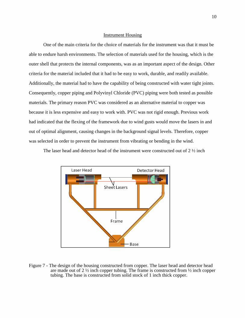
Velocity

The new prototype measures the velocity and diameter of hydrometeors. Gunn and

Kinzer performed lab experiments to obtain benchmark data for the relationship between drop

diameter and terminal velocity (Gunn & Kinzer, 1949). The measured data for each precipitation

event was compared against the Gunn and Kinzer Relationship as shown in Figure 32, Figure 33,

and Figure 34.

Figure 32 - A comparison of the measured velocities during a thunderstorm captured on February 29th, 2012 against the theoretical Gunn and Kinzer Relationship. The scatter of the measured data is mostly likely due to the dynamic environment in which the measurements were taken.

44

Figure 33 - The velocities of snowflakes compared against the Gunn & Kinzer Relationship.

Figure 34 - The velocities measured during the March 12th rain event compared against the Gunn & Kinzer Relationship.

45

Discussion

Figure 29 and Figure 30 show that the new prototype detects rain at the same time as the

tipping bucket, but the prototype does not signal snow at the same time as the tipping bucket.

The tipping bucket was not designed to measure precipitation in the form of snow. The tipping

bucket does signal precipitation during hour 20:00 on February 29th

. The signal is due to the

snow being trapped in the tipping bucket and melting which caused the tipping bucket to tip

once.

The prototype consistently underestimates the magnitude of the rain rates compared to

the rain rates captured by the tipping bucket. The two largest sources of errors leading to the

underestimation is multiple drops in the sample area while another drop is being measured, and

the limitation of not being able to estimate hydrometeors less than or equal to 0.9 millimeters.

Another factor that may lead to consistent underestimation of rain rates is over estimation of the

sample area. The sample area used is based upon the size the area between the detector head and

lasers head. Because the laser diverges slightly, light in some areas is headed out of the sample

area and is never detected by the detector. Similarly, light near the edges is not focused on the

detector. Thus the sample is somewhat smaller than our estimate.

In order to capture small drops with slower velocities the prototype’s settings were set to

record 1500 measurements at a frequency of 66.6 kHz. Therefore, every time the prototype

sensed a hydrometeor, there is a 0.0225 second window of time that another drop can enter the

sampling area. An example of two drops being measured during one window of time can be seen

in Figure 35. If more than one drop is recorded during this window of time, both of the drops

were eliminated as errors. Errors of this type are referred to as simultaneous drops. Therefore, for

every error due to simultaneous drops, two or more drops are not being included in the drop size

distribution. The probability of this happening increases with increased rain intensity, which

explains the larger differences between the rain rates measured by the prototype and tipping

bucket during higher rain rates.

46

The number of drops analyzed as errors during the February 29th

and March 12th

rain

events are shown in Table 5. Table 6 shows the number errors associated with simultaneous

drops in the sample area and errors due to drops equal to or smaller than 0.90 mm.

Table 5 - The number of triggers and errors associated with each rain event.

Rain Event Number of Total Number Total Number of % of Triggers

Day Hours Triggers of Errors Drops Analyzed as Errors

February 29th 0-2 10252 3269 6983 32

March 12th 8:00 - 10:45 5094 1378 3716 27

Figure 35 - An example of another drop entering the sample area during the same window of time a measurement takes place.

47

Table 6 - A table breaking down the number of simultaneous drops in the sample area and the number of drops smaller than 0.90 mm not included in the DSD.

Assuming that the number of simultaneous drops entering the sample area counts for two

drops, the number of drops not included in the drop size distribution during the February 29th

rain event is 5753. Therefore, the corrected number of drops that fell through the sample area is

12736. This means 45 percent of the drops recorded were eliminated as errors during the

February 29th

rain storm. This is a conservative estimate since it is assumed that only two drops

were in the sample area when simultaneous drops were recorded. Using the same logic it was

estimated that 37 percent of the drops during the March 12th

rainstorm were not analyzed. This is

consistent with the observation that the new prototype underestimates rain rates by just over a

factor of 2.

The percentage of the total errors from drops with diameters less than 0.90 mm was 32

percent and 77 percent for the February 29th

and March 12th

rain events respectively. A possible

reason for this difference is due to the type of rain event that occurred. The March 12th

rain event

was a light stratiform rain while the rain event on February 29th

was a thunderstorm. Light

stratiform precipitation is characterized by smaller drops while thunderstorms or convective

storms have larger rain drops.

Another source of uncertainty is the assumption that the shapes of all rain drops are

perfect spheres. Raindrops smaller than 1 millimeter are usually perfect spheres since

intermolecular forces are strong enough to hold the drop in the shape of a sphere. As the size of

raindrops increases, the drag force acting on the raindrops increases because of the larger frontal

area. Thus the shapes of raindrops are deformed. The bottom edge of the raindrop becomes flat

Rain Event Errors Due to Errors Due to Drops

Day Hours Simultaneous Drops Smaller than 0.90 mm

February 29th 0:00 - 2:00 2484 785

March 12th 8:00 - 10:45 778 600

48

while the lateral length of the raindrop elongates. The top of the drop remains rounded. The

shape resembles a mushroom with no stem. The new prototype measures the longitudinal

(vertical) length of raindrops which becomes shorter when rain drops are deformed. Using the

longitudinal length and assuming the rain drop is a sphere leads to the underestimation of the true

rain drop volume. A study by (Jones, 1959) showed that the average ratio between the

longitudinal length and lateral length of a 2 mm drop was 0.99; a 3 mm drop was 0.92; and a 4

mm drop was 0.85. Assuming a 3 mm drop diameter is underestimated by 4 percent, half the

difference of the ratio (longitudinal to lateral length) from one for a 3mm drop found by Jones

would lead to a 12 percent underestimation of the volume for a drop.

The velocities of the hydrometeors measured by the new prototype fell closely to the

theoretical Gunn and Kinzer relationship for the February 29th

and March 12th

rain events. The

Gunn and Kinzer Relationship was determined in a laboratory in stagnant air whereas the

velocity measurements recorded by the prototype were taken outdoors in an dynamic enviroment

where updrafts, and downdrafts occur. An updraft would decrease the measured velocity while a

downdraft would increase the velocity. Therefore, the scatter in the velocity measurements was

expected. The velocities measured during the snow event were much lower than the Gunn and

Kinzer Relationship. This was expected since snow flakes are less areodynamic and less dense

than water droplets .

Outdoor Testing Conclusions

The prototype was placed outdoors on the roof of the Wind Tunnel Annex from February

20th

to March 13th

. Two rain events and one snow event were captured by the prototype. The new

prototype underestimated the rain rates compared to the rain rates measured by the tipping

bucket by a factor of just over two. Furthermore the prototype’s underestimation of the measured

rain rates increased with increased rain rates. Rain drops smaller than 0.90 mm and drops

occupying the sample area simultaneously were the two main errors contributing to the

underestimation of the rain rates. It was estimated that 45 percent of the drops were not analyzed

49

during the February 29th

rain event, and 37 percent of the drops were not analyzed during the

March 12th

rain event.

The velocities measured by the new prototype compared well with the relationship

developed by Gunn and Kinzer. The scatter in the measured data was expected due to the

dynamic environment in which the measurements were taken.

50

CHAPTER 7

CONCLUSION

A new instrument that measures the diameter and velocity of hydrometeors was

redesigned, constructed, and tested. The redesigned instrument was based off of previous

prototypes built by Michael Cloos. The new prototype has the advantage of being able to be

repaired or adjusted if an internal component fails or becomes misaligned. Additionally a new

data analysis method was developed during this project. The instrument and data analysis

method were tested after the instrument was constructed.

Two controlled lab experiments were performed to assess the accuracy and precision of

velocity and diameter estimates made by the new prototype. The first experiment consisted of

dropping one hundred and fifty steel spheres with diameters of 0.98 mm, 1.98 mm, 2.98 mm,

3.98 mm, 4.98 mm, and 5.98 mm through the sample area of the new prototype. The 0.98 mm

diameter spheres had a 12.4 percent average fractional error, the largest of the diameters tested.

The 5.98 mm diameter spheres had the lowest average fractional error, 1.89 percent. The average

fractional error decreased with increasing diameter size.

The average error of the velocity measurements compared to the calculated theoretical

velocity ranged from -3.3 to -0.27 percent. The primary reason the measured velocities are

slightly lower than the theoretical velocities was because the drag force was assumed zero in the

theoretical calculations. The 0.98 mm trials had the largest average error of -3.3 percent. The

0.98 mm spheres were dropped by hand from a lower height since the mechanical device did not

work for the 0.98 mm spheres. The fractional percent errors of the velocity measurements for

each diameter tested ranged from 0.58 to 0.84 percent which was in good agreement with the

estimated fractional error of 0.5 percent.

The second lab experiment performed was the Drip Experiment. The Drip Experiment

consisted of dropping 25 milliliters of water through the sample area in the form of water

droplets. The estimated volumes from all 22 trials underestimated the actual volume of water by

51

an average of 2.7 mL ±1.18 mL. The average error was 10.79 percent which was reasonable

considering that any errors in estimating the diameters are magnified to the power of three and

summed over an average of 476 drops per trial.

Lastly, the instrument was placed outside to test the durability of the instrument, and to

assess the accuracy of the instrument during precipitation events. The instrument was placed on

the roof the University of Iowa Wind Tunnel Annex from February 20th

, 2012 to March 14th

,

2012 approximately 30 feet from an Iowa Flood Center Tipping Bucket. The new prototype

never failed mechanically because of the elements while being outdoors. Two rain events and

one snow event were captured during the outdoor campaign. The new prototype signaled

precipitation at the same times as the tipping bucket but underestimated the magnitude of the

rain rates compared to the tipping bucket by a factor just over 2. The primary reasons for the

underestimation were due to errors from multiple drops occupying the sample area

simultaneously and the data analysis limitation of not being able to estimate diameters smaller

than or equal to 0.90 mm. The new prototype did signal precipitation during the snow event

while the tipping bucket did not. The tipping bucket was not designed to measure snow. The

diameters of the hydrometeors measured during the snow event had no meaning since the

relationship between the size of a snowflake and the pulsed signals has not been investigated.

The velocities from the two rain events and the snow events were compared against Gunn

and Kinzer Relationship which relates the terminal velocity of droplets to their diameter. The

two rain events agreed well with the theoretical relationship while the majority of the velocities

estimated during the snow event were smaller than the theoretical Gunn and Kinzer curve. This

was expected since snowflakes are less aerodynamic and less dense than water droplets. The

scatter of the data most likely occurred from the measurements being measured in a dynamic

environment where downdrafts and updrafts happen. The upward or downward movement of air

affects the velocities of hydrometeors.

The lab experiments and outdoor testing periods are evidence that the new prototype is

capable of measuring the velocities and diameters of hydrometeors. However, over the duration

52

of this project, additional issues with the data collection, data analysis, and instrument were

identified. To further improve the instrument the following issues should be addressed.

Issues to Be Addressed

The first issue that should be addressed is increasing the signal to noise ratio. This could

be done by performing a DC offset on the signal to remove the background noise and then

amplifying the signal. This would enhance the processing of the raw data by removing the

ambiguity when determining the time of attenuation or the half-max time of attenuation. In

particular, increasing the signal to noise ratio would enhance the ability to process drops equal to

or smaller than 0.90 mm. The small pulsed signals should not be stair stepped shaped and could

be analyzed by fitting Equation 4.18 to the end of the pulsed signals as described in Chapter 4.

Furthermore, by increasing the signal to noise ratio, the accuracy of determining the time of

attenuation, tatt, from the raw data could possibly be increased. Then the theoretical diameter

calculation method described in Chapter 4 could be used to estimate the diameters. The

advantage of the theoretical diameter calculation method is that a data reduction curve would not

have to be developed.

The next issue that needs to be resolved is the errors associated with two or more rain

drops occupying the sample area simultaneously. Currently, when the instrument detects a

hydrometeor in the sample area, the data collection algorithm takes 1500 measurements at a

frequency of 66.6 kHz. This creates dead time of 0.0225 seconds after each hydrometeor enters

the sampling area. Previous work by Cloos indicated that taking 500 measurements was too short

because, for very small drops, the second pulsed signal corresponding to a hydrometeor passing

through the second laser sheet was not recorded by the instrument. This error was more prevalent

for small hydrometeors because small hydrometeors tend to have slower velocities, which in turn

take more time to pass by both laser sheets. In order to decrease the number of these errors, an

improved data collection algorithm needs to be developed. One idea is to have the data collection

algorithm quit taking samples after the second pulsed signal is fully captured. This would reduce

53

the dead time which would reduce the probability of multiple drops being measured during the

same window of time. Another idea is to include a dead time analysis as Knoll describes in his

book Radiation Detection & Measurement in order to account for the hydrometeors not being

measured during the dead time.

Lastly, a detailed map of the actual sample area of laser light the photo detector sees

should be developed. As of now the sample area was taken as the area between the detector head

and laser head. It is hypothesized that the sample area could be smaller than the sample area used

during this project. The divergence of some of the laser light near the edges is headed out of the

sample area and is never detected by the photo detector. Similarly, light near the edge of the

sample area is not focused on the detector. Understanding the actual sample area seen by the

photo detector will remove one more of the uncertainties.

In conclusion, a new instrument that measures precipitation was designed, constructed,

and tested. The instrument was capable of measuring the diameter and velocity of individual

raindrops during precipitation events. The prototype has the potential to become a useful

meteorological instrument by resolving the issues discovered over the duration of this project.

54

BIBLIOGRAPHY

Cloos, M. P. (2007). Measuring Hydrometeor Size, Shape, and Vlocity Using A New Non-Video,

Two - Dimensional Disdrometer. Iowa City.

Frasson, R., Cunha, L., & Krajewski, W. (2011). Assessment of the Thies optical disdrometer

performance. Atmospheric Research, 237-255.

Gunn, R., & Kinzer, G. (1949). The Terminal Velocity for Water Droples in Stagnant Air.

Journal of Meteorology, 243-248.

History for Iowa City, IA. (2012, February 29). Retrieved March 5, 2012, from

http://www.wunderground.com/history/airport/KIOW/2012/2/29/DailyHistory.html?req_

city=NA&req_state=NA&req_statename=NA

History for Iowa City, IA. (2012, March 12). Retrieved March 14, 2012, from

http://www.wunderground.com/history/airport/KIOW/2012/3/12/DailyHistory.html?req_

city=NA&req_state=NA&req_statename=NA

Jones, D. M. (1959). The Shape of Raindrops. Journal of Meteorology, 504-510.

Knoll, F. G. (1989). Radiation Detection and Measurement. New York: John Wiley and Sons.

Kruger, A., & Krajewski, W. (2001). Two-Dimensional Video Disdrometer: A Discription.

Atmospheric and Oceanic Technology, 602 - 617.

Kruger, A., Krajewski, W. F., & Kucera, P. A. (2002). Measurements of drop size distribution in

the southwestern Amazon Basin. Journal of Geophysical Research, 19.1-19.15.

List, R. (1988). A linear radar reflectivity -rainrate relationship for steady tropical rain. Journal

of Atmospheric Science, 3564-3572.

Loffler-Mang, M. (1998). An Optical Disdrometer for Measuring Size and Velocity of

Hydrometeors. Atmospheric and Oceanic Technology, 130 - 139.

Nespor, V., Krajewski, W., & Kruger, A. (2000). Wind-Induced Error of Raindrop Size

Disdribution Measurements Using a Two-Dimensional Video Disdrometer. Atmospheric

and Oceanic Technology, 1483 - 1492.

Thies Clima, Laser Precipitation Monitor (Disdrometer). (n.d.). Retrieved February 2012, from

http://www.thiesclima.com/disdrometer.html

Tokay, A., Kruger, A., & Krajewski, W. F. (2001). Comparison of Drop Size Distribution

Measurements by Impact and Optical Disdrometers. Journal of Applied Meteorology,

2083-2097.

55

Tokay, T., Kruger, A., Kucera, P., Krajewski, W., & Pereira Filho, A. (2002). Measurements of

drop size distribution in the southwestern Amazon Basin. Geophysical Research, 19.5 -

19.15.