A reconstruction of radiocarbon production and total solar ... · bon and carbon isotopes. The...
31
Clim. Past, 9, 1879–1909, 2013 www.clim-past.net/9/1879/2013/ doi:10.5194/cp-9-1879-2013 © Author(s) 2013. CC Attribution 3.0 License. Climate of the Past Open Access A reconstruction of radiocarbon production and total solar irradiance from the Holocene 14 C and CO 2 records: implications of data and model uncertainties R. Roth and F. Joos Climate and Environmental Physics, Physics Institute, University of Bern, Bern, Switzerland Oeschger Centre for Climate Change Research, University of Bern, Bern, Switzerland Correspondence to: R. Roth ([email protected]) Received: 7 February 2013 – Published in Clim. Past Discuss.: 1 March 2013 Revised: 5 June 2013 – Accepted: 7 June 2013 – Published: 9 August 2013 Abstract. Radiocarbon production, solar activity, total solar irradiance (TSI) and solar-induced climate change are re- constructed for the Holocene (10 to 0 kyr BP), and TSI is predicted for the next centuries. The IntCal09/SHCal04 ra- diocarbon and ice core CO 2 records, reconstructions of the geomagnetic dipole, and instrumental data of solar activity are applied in the Bern3D-LPJ, a fully featured Earth system model of intermediate complexity including a 3-D dynamic ocean, ocean sediments, and a dynamic vegetation model, and in formulations linking radiocarbon production, the solar modulation potential, and TSI. Uncertainties are assessed us- ing Monte Carlo simulations and bounding scenarios. Tran- sient climate simulations span the past 21 thousand years, thereby considering the time lags and uncertainties associ- ated with the last glacial termination. Our carbon-cycle-based modern estimate of radiocarbon production of 1.7 atoms cm -2 s -1 is lower than previously reported for the cosmogenic nuclide production model by Masarik and Beer (2009) and is more in-line with Kovaltsov et al. (2012). In contrast to earlier studies, periods of high solar activity were quite common not only in recent millen- nia, but throughout the Holocene. Notable deviations com- pared to earlier reconstructions are also found on decadal to centennial timescales. We show that earlier Holocene recon- structions, not accounting for the interhemispheric gradients in radiocarbon, are biased low. Solar activity is during 28% of the time higher than the modern average (650 MeV), but the absolute values remain weakly constrained due to un- certainties in the normalisation of the solar modulation to instrumental data. A recently published solar activity–TSI relationship yields small changes in Holocene TSI of the or- der of 1 W m -2 with a Maunder Minimum irradiance reduc- tion of 0.85 ± 0.16 W m -2 . Related solar-induced variations in global mean surface air temperature are simulated to be within 0.1 K. Autoregressive modelling suggests a declining trend of solar activity in the 21st century towards average Holocene conditions. 1 Introduction Solar insolation is the driver of the climate system of the earth (e.g. Gray et al., 2010; Lockwood, 2012). Variations in total solar irradiance (TSI) have the potential to signif- icantly modify the energy balance of the earth (Crowley, 2000; Ammann et al., 2007; Jungclaus et al., 2010). How- ever, the magnitude of variations in TSI (Schmidt et al., 2011, 2012; Shapiro et al., 2011; Lockwood, 2012) and its tempo- ral evolution (Solanki et al., 2004; Muscheler et al., 2005b; Schmidt et al., 2011) remain uncertain and are debated. Solar activity and TSI were reconstructed from the Holocene radio- carbon record. These reconstructions relied on box models of the ocean and land carbon cycle or on a 2-D representation of the ocean (Solanki et al., 2004; Marchal, 2005; Usoskin and Kromer, 2005; Vieira et al., 2011; Steinhilber et al., 2012). However, a quantification of how past changes in climate and the carbon cycle affect reconstructions of radiocarbon production and solar activity is yet missing. Aspects ne- glected in earlier studies include (i) changes in the climate– carbon-cycle system over the last glacial termination (∼ 18 to Published by Copernicus Publications on behalf of the European Geosciences Union.
Transcript of A reconstruction of radiocarbon production and total solar ... · bon and carbon isotopes. The...
Clim. Past, 9, 1879–1909, 2013www.clim-past.net/9/1879/2013/doi:10.5194/cp-9-1879-2013© Author(s) 2013. CC Attribution 3.0 License.
EGU Journal Logos (RGB)
Advances in Geosciences
Open A
ccess
Natural Hazards and Earth System
Sciences
Open A
ccess
Annales Geophysicae
Open A
ccess
Nonlinear Processes in Geophysics
Open A
ccess
Atmospheric Chemistry
and Physics
Open A
ccess
Atmospheric Chemistry
and PhysicsO
pen Access
Discussions
Atmospheric Measurement
Techniques
Open A
ccess
Atmospheric Measurement
Techniques
Open A
ccess
Discussions
Biogeosciences
Open A
ccess
Open A
ccess
BiogeosciencesDiscussions
Climate of the Past
Open A
ccess
Open A
ccess
Climate of the Past
Discussions
Earth System Dynamics
Open A
ccess
Open A
ccess
Earth System Dynamics
Discussions
GeoscientificInstrumentation
Methods andData Systems
Open A
ccess
GeoscientificInstrumentation
Methods andData Systems
Open A
ccess
Discussions
GeoscientificModel Development
Open A
ccess
Open A
ccess
GeoscientificModel Development
Discussions
Hydrology and Earth System
Sciences
Open A
ccess
Hydrology and Earth System
Sciences
Open A
ccess
Discussions
Ocean Science
Open A
ccess
Open A
ccess
Ocean ScienceDiscussions
Solid Earth
Open A
ccess
Open A
ccess
Solid EarthDiscussions
The Cryosphere
Open A
ccess
Open A
ccess
The CryosphereDiscussions
Natural Hazards and Earth System
Sciences
Open A
ccess
Discussions
A reconstruction of radiocarbon production and total solarirradiance from the Holocene14C and CO2 records: implications ofdata and model uncertainties
R. Roth and F. Joos
Climate and Environmental Physics, Physics Institute, University of Bern, Bern, Switzerland
Oeschger Centre for Climate Change Research, University of Bern, Bern, Switzerland
Correspondence to:R. Roth ([email protected])
Received: 7 February 2013 – Published in Clim. Past Discuss.: 1 March 2013Revised: 5 June 2013 – Accepted: 7 June 2013 – Published: 9 August 2013
Abstract. Radiocarbon production, solar activity, total solarirradiance (TSI) and solar-induced climate change are re-constructed for the Holocene (10 to 0 kyr BP), and TSI ispredicted for the next centuries. The IntCal09/SHCal04 ra-diocarbon and ice core CO2 records, reconstructions of thegeomagnetic dipole, and instrumental data of solar activityare applied in the Bern3D-LPJ, a fully featured Earth systemmodel of intermediate complexity including a 3-D dynamicocean, ocean sediments, and a dynamic vegetation model,and in formulations linking radiocarbon production, the solarmodulation potential, and TSI. Uncertainties are assessed us-ing Monte Carlo simulations and bounding scenarios. Tran-sient climate simulations span the past 21 thousand years,thereby considering the time lags and uncertainties associ-ated with the last glacial termination.
Our carbon-cycle-based modern estimate of radiocarbonproduction of 1.7 atoms cm−2 s−1 is lower than previouslyreported for the cosmogenic nuclide production model byMasarik and Beer(2009) and is more in-line withKovaltsovet al. (2012). In contrast to earlier studies, periods of highsolar activity were quite common not only in recent millen-nia, but throughout the Holocene. Notable deviations com-pared to earlier reconstructions are also found on decadal tocentennial timescales. We show that earlier Holocene recon-structions, not accounting for the interhemispheric gradientsin radiocarbon, are biased low. Solar activity is during 28 %of the time higher than the modern average (650 MeV), butthe absolute values remain weakly constrained due to un-certainties in the normalisation of the solar modulation toinstrumental data. A recently published solar activity–TSI
relationship yields small changes in Holocene TSI of the or-der of 1 W m−2 with a Maunder Minimum irradiance reduc-tion of 0.85± 0.16 W m−2. Related solar-induced variationsin global mean surface air temperature are simulated to bewithin 0.1 K. Autoregressive modelling suggests a decliningtrend of solar activity in the 21st century towards averageHolocene conditions.
1 Introduction
Solar insolation is the driver of the climate system of theearth (e.g.Gray et al., 2010; Lockwood, 2012). Variationsin total solar irradiance (TSI) have the potential to signif-icantly modify the energy balance of the earth (Crowley,2000; Ammann et al., 2007; Jungclaus et al., 2010). How-ever, the magnitude of variations in TSI (Schmidt et al., 2011,2012; Shapiro et al., 2011; Lockwood, 2012) and its tempo-ral evolution (Solanki et al., 2004; Muscheler et al., 2005b;Schmidt et al., 2011) remain uncertain and are debated. Solaractivity and TSI were reconstructed from the Holocene radio-carbon record. These reconstructions relied on box models ofthe ocean and land carbon cycle or on a 2-D representation ofthe ocean (Solanki et al., 2004; Marchal, 2005; Usoskin andKromer, 2005; Vieira et al., 2011; Steinhilber et al., 2012).
However, a quantification of how past changes in climateand the carbon cycle affect reconstructions of radiocarbonproduction and solar activity is yet missing. Aspects ne-glected in earlier studies include (i) changes in the climate–carbon-cycle system over the last glacial termination (∼ 18 to
Published by Copernicus Publications on behalf of the European Geosciences Union.

1880 R. Roth and F. Joos: A reconstruction of radiocarbon production and total solar irradiance
11 kyr BP), (ii) variations in Holocene and last millenniumclimate, (iii) changes in ocean sediments, and (iv) changes invegetation dynamics and in anthropogenic land use.
The goal of this study is to reconstruct Holocene radio-carbon production, solar modulation potential to characterisethe open solar magnetic field, TSI, and the influence of TSIchanges on Holocene climate from the proxy records of at-mospheric114C (McCormac et al., 2004; Reimer et al.,2009) and CO2 and a recent reconstruction of the geomag-netic field (Korte et al., 2011). The TSI reconstruction is ex-tended into the future to year 2300 based on its spectral prop-erties. We apply the Bern3D-LPJ Earth system model of in-termediate complexity that features a 3-D dynamic ocean, re-active ocean sediments, a dynamic global vegetation model,an energy–moisture balance atmosphere, and cycling of car-bon and carbon isotopes. The model is forced by changes inorbital parameters, explosive volcanic eruptions, well-mixedgreenhouse gases (CO2, CH4, N2O), aerosols, ice cover andland-use area changes. Bounding scenarios for deglacial ra-diocarbon changes and Monte Carlo techniques are appliedto comprehensively quantify uncertainties.
TSI reconstructions that extend beyond the satellite recordmust rely on proxy information.14C and 10Be are twoproxies that are particularly well suited (Beer et al., 1983;Muscheler et al., 2008; Steinhilber et al., 2012); their produc-tion by cosmic particles is directly modulated by the strengthof the solar magnetic field and they are conserved in ice cores(10Be) and tree rings (14C). The redistributions of10Be and14C within the climate system follow very different path-ways, and thus the two isotopes can provide independentinformation. The10Be and14C proxy records yield in gen-eral consistent reconstructions of isotope production and so-lar activity with correlations exceeding 0.8 (Bard et al., 1997;Lockwood and Owens, 2011). Important caveats, however,and differences in detail remain. After production,10Be isattached to aerosols, and variations in atmospheric transportand dry and wet deposition of10Be and incorporation intothe ice archive lead to noise and uncertainties. This is high-lighted by the opposite, and not yet understood, 20th cen-tury trends in10Be in Greenland versus Antarctic ice cores(Muscheler et al., 2007; Steinhilber et al., 2012). Thus, takenat face value, Greenland and Antarctic10Be records suggestopposite trends in solar activity in the second half of the20th century.
14C is oxidised after production and becomes as14CO2part of the global carbon cycle. It enters the ocean, sedi-ments, and the land biosphere and is removed from the cli-mate system by radioactive decay, with an average lifetime of5730 yr/ln(2) = 8267 yr, and to a minor part by seafloor sedi-ment burial. Atmospheric14C is influenced not only by short-term production variations, but also by variations of the cou-pled carbon-cycle–climate system, and their evolutions dueto the long timescales governing radioactive decay and car-bon overturning in the land and ocean.
The conversion of the radiocarbon proxy record(McCormac et al., 2004; Reimer et al., 2009) to TSIinvolves several steps. First a carbon cycle model is appliedto infer radiocarbon production by deconvolving the atmo-spheric radiocarbon budget. Radiocarbon production is equalto the prescribed changes in the atmospheric radiocarboninventory and decay in the atmosphere plus the modelled netair-to-sea and net air-to-land14C fluxes. The radiocarbonsignature of a flux or a reservoir is commonly reported inthe114C notation, i.e. as the fractionation-corrected per mildeviation of 14R = 14C/12C from a given standard definedas 14Rstd= 1.176× 10⁻¹² (Stuiver and Polach, 1977). 14Cproduction depends on the magnitude of the shielding ofthe earth’s atmosphere by the geomagnetic and the opensolar magnetic fields. Reconstructions of the geomagneticfield can thus be combined with a physical cosmogenicisotope production model (Masarik and Beer, 1999, 2009;Kovaltsov et al., 2012) to infer the strength of the magneticfield enclosed in solar winds as expressed by the so-calledsolar modulation potential,8. Finally, 8 is translated intovariations in TSI.
Each of these steps has distinct uncertainties and chal-lenges. Deglacial carbon cycle changes are large, and at-mospheric CO2 increased from 180 ppm at the Last GlacialMaximum (LGM) to 265 ppm 11 kyr BP. These variations arethought to be driven by physical and biogeochemical reor-ganisations of the ocean (e.g.Brovkin et al., 2012; Menvielet al., 2012). They may influence the14C evolution in theHolocene and the deconvolution for the14C production, butwere not considered in previous studies. Many earlier stud-ies (Marchal, 2005; Muscheler et al., 2005a; Usoskin andKromer, 2005; Vonmoos et al., 2006; Steinhilber et al., 2012)deconvolving the14C record relied on simplified box mod-els using a perturbation approach (Oeschger et al., 1975;Siegenthaler, 1983) where the natural marine carbon cycleis not simulated and climate and ocean circulations as wellas land carbon turnover are kept constant. In the perturba-tion approach, the ocean carbon and radiocarbon inventory isunderestimated by design as the concentration of dissolvedinorganic carbon is set to its surface concentration.12C and14C are not transported as separate tracers but combined intoa single tracer, the14C/12C ratio. These shortcomings, how-ever, can be overcome by applying a spatially resolved cou-pled carbon-cycle–climate model that includes the naturalcarbon cycle and its anthropogenic perturbation, and where12C and14C are distinguished.
A key target dataset is the data of the Global Ocean DataAnalysis Project (GLODAP) that includes station data andgridded data of dissolved inorganic carbon and its14C signa-ture (Key et al., 2004). This permits the quantification of theoceanic radiocarbon inventory, by far the largest radiocarboninventory on earth. Together with data-based estimates of thecarbon inventory on land, in the atmosphere, and in reactivesediment and their signatures, the global radiocarbon inven-tory and thus the long-term average14C production can be
Clim. Past, 9, 1879–1909, 2013 www.clim-past.net/9/1879/2013/

R. Roth and F. Joos: A reconstruction of radiocarbon production and total solar irradiance 1881
reliably estimated. Further, the spatial carbon and14C dis-tribution within the oceans is a yard stick to gauge the per-formance of any ocean circulation and carbon cycle model.14C permits the quantification of the overturning timescaleswithin the ocean (e.g.Muller et al., 2006) and of the mag-nitude of the air–sea carbon exchange rate (e.g.Naegler andLevin, 2006; Sweeney et al., 2007; Muller et al., 2008).
The conversion of the radiocarbon production record into8 requires knowledge on the strength of the geomagneticfield, which together with the open solar magnetic field con-tributes to the shielding of the earth’s atmosphere from thecosmic ray flux. Recently, updated reconstructions of theearth magnetic field have become available (Knudsen et al.,2008; Korte et al., 2011). The palaeo-proxy record of8should be consistent with instrumental observations. The de-convolution of the atmospheric14C history for natural pro-duction variations is only possible up to about 1950 AD. Af-terwards, the atmospheric14C content almost doubled dueto atomic bomb tests in the fifties and early sixties of the20th century and uncertainties in this artificial14C produc-tion are larger than natural production variations. This lim-its the overlap of the14C-derived palaeo-proxy record of8 with reconstructions of8 based on balloon-borne mea-surements and adds uncertainty to the normalisation of thepalaeo-proxy record to recent data. How variations in cosmo-genic isotope production and in8 are related to TSI is un-clear and there is a lack of understanding of the mechanisms.This is also reflected in the large spread in past and recentreconstructions of TSI variability on multi-decadal to cen-tennial timescales (e.g.Bard et al., 2000; Lean, 2000; Wanget al., 2005; Steinhilber et al., 2009; Steinhilber et al., 2012;Shapiro et al., 2011; Schrijver et al., 2011). Recent recon-structions based on the decadal-scale trend found in the TSIsatellite record reveal small amplitude variations in TSI ofthe order of 1 W m−2 over past millennia (Steinhilber et al.,2009), whereas others based on observations of the mostquiet area on the present sun suggest that TSI variations areof the order of 6 W m−2 or even more (Shapiro et al., 2011).
The outline of this study is as follows. Next, we will de-scribe the carbon cycle model and methods applied. In theresults Sect. 3, we apply sinusoidal variations in atmospheric14C with frequencies between 1/(5 yr) to 1/(1000 yr). The re-sults characterise the model response to a given radiocarbontime series as any time series can be described by its powerspectrum using Fourier transformation.
In Sect. 3.2, we discuss the radiocarbon and carbon in-ventory and distribution in the model in comparison withobservations (Sect. 3.1), before turning to the time evolu-tion of the carbon fluxes, the atmospheric carbon budget, andradiocarbon production in Sect. 3.2. In Sects. 3.3 to 3.5 re-sults are presented for the solar activity, TSI, and simulated,solar-driven changes in global mean surface air temperatureover the Holocene and extrapolated TSI variations up to year2300. Discussion and conclusions follow in Sect. 4 and the
Appendix presents error calculations for14C production, so-lar modulation, and TSI in greater detail.
2 Methodology
2.1 Carbon cycle model description
The Bern3D-LPJ climate–carbon-cycle model is an Earthsystem model of intermediate complexity and includes anenergy and moisture balance atmosphere and sea ice model(Ritz et al., 2011), a 3-D dynamic ocean (Muller et al., 2006),a marine biogeochemical cycle (Tschumi et al., 2008; Parekhet al., 2008), an ocean sediment model (Tschumi et al., 2011),and a dynamic global vegetation model (Sitch et al., 2003)(Fig. 1). Total carbon and the stable isotope13C and the ra-dioactive isotope14C are transported individually as tracersin the atmosphere–ocean-sediment–land biosphere system.
The geostrophic-frictional balance 3-D ocean componentis based onEdwards and Marsh(2005) and as further im-proved byMuller et al.(2006). It includes an isopycnal diffu-sion scheme and Gent-McWilliams parametrisation for eddy-induced transport (Griffies, 1998). Here, a horizontal reso-lution of 36× 36 grid boxes and 32 layers in the verticalis used. Wind stress is prescribed according to the monthlyclimatology from NCEP/NCAR (Kalnay et al., 1996). Thus,changes in ocean circulation in response to changes in windstress under varying climate are not simulated.
The atmosphere is represented by a 2-D energy and mois-ture balance model with the same horizontal resolution asthe ocean (Ritz et al., 2011). FollowingWeaver et al.(2001),outgoing long-wave radiative fluxes are parametrised afterThompson and Warren(1982) with additional radiative forc-ings due to CO2, other greenhouse gases, volcanic aerosols,and a feedback parameter, chosen to produce an equilibriumclimate sensitivity of 3◦C for a nominal doubling of CO2.The past extent of Northern Hemisphere ice sheets is pre-scribed following the ICE4G model (Peltier, 1994) as de-scribed inRitz et al.(2011).
The marine biogeochemical cycling of carbon, alkalinity,phosphate, oxygen, silica, and of the carbon isotopes is de-tailed by Parekh et al.(2008) and Tschumi et al.(2011).Remineralisation of organic matter in the water column aswell as air–sea gas exchange is implemented according tothe OCMIP-2 protocol (Orr and Najjar, 1999; Najjar et al.,1999). However, the piston velocity now scales linear (in-stead of a quadratic dependence) with wind speed follow-ing Krakauer et al.(2006). The global mean air–sea trans-fer rate is reduced by 17 % compared to OCMIP-2 to matchobservation-based estimates of natural and bomb-producedradiocarbon (Muller et al., 2008), and is in agreement withother studies (Sweeney et al., 2007; Krakauer et al., 2006;Naegler and Levin, 2006). As fractionation of14CO2 is nottaken into account during air–sea gas exchange, the air–seafluxes are corrected in postprocessing using13C, for which
www.clim-past.net/9/1879/2013/ Clim. Past, 9, 1879–1909, 2013

1882 R. Roth and F. Joos: A reconstruction of radiocarbon production and total solar irradiance
GHGs radiative forcingSO4 aerosols forcingice-sheet extent/albedoorbital parameters
energy & moisture balance model
0° 60°E120°E 180° 120°W 60°W 0°
temperatureprecipitationirradiance
atmosphere (12C,14C)radiocarbon production
radiocarbon decay
14Fas12Fab
14Fab
radiocarbon decay & burial radiocarbon
decay
land
0.0 1.8 3.6
carbon cycle model0° 60°E 120°E 180°120°W 60°W 0°
ice core CO2
Q
ocean
0.0 5.0 10.0
12Fas
carbon burial
IntCal/SHCal Δ14C
Fig. 1. Setup of the Bern3D-LPJ carbon-cycle–climate model. Grey arrows denote externally applied forcings resulting from variations ingreenhouse gas concentrations and aerosol loading, orbital parameters, ice sheet extent, sea level and atmospheric CO2 and114C. Theatmospheric energy and moisture balance model (blue box and arrows) communicates interactively the calculated temperature, precipitationand irradiance to the carbon cycle model (light brown box). The production and exchange fluxes of radiocarbon (red) and carbon (green)within the carbon cycle model are sketched by arrows, where the width of the arrows indicates the magnitude of the corresponding fluxesin a preindustrial steady state. The two maps show the depth-integrated inventories of the preindustrial14C content in the ocean and landmodules in units of 103 mol14C m−2/14Rstd.
the fractionation is explicitly calculated in the model. Prog-nostic formulations link marine productivity and export pro-duction of particulate and dissolved organic matter (POM,DOM) to available nutrients (P, Fe, Si), temperature, andlight in the euphotic zone. Carbon is represented as trac-ers of dissolved inorganic carbon (DIC), DIC-13 and DIC-14, and labile dissolved organic carbon (DOC), DOC-13 andDOC-14. Particulate matter (POM and CaCO3) is reminer-alised/dissolved in the water column applying a Martin-typepower-law curve.
A 10-layer sediment diagenesis model (Heinze et al.,1999; Gehlen et al., 2006) is coupled to the oceanfloor, dynamically calculating the advection, remineralisa-tion/redissolution and bioturbation of solid material in thetop 10 cm (CaCO3, POM, opal and clay), as well as pore-water chemistry and diffusion as described in detail inTschumi et al.(2011). In contrast to the setup inTschumiet al. (2011), the initial alkalinity inventory in the ocean isincreased from 2350 to 2460 µmol kg−1 in order to get a re-alistic present-day DIC inventory (Key et al., 2004).
The land biosphere model is based on the Lund–Potsdam–Jena (LPJ) dynamic global vegetation model with a res-olution of 3.75◦ × 2.5◦ as used inJoos et al. (2001),Gerber et al.(2003), Joos et al.(2004) and described in de-tail in Sitch et al.(2003). The fertilisation of plants by CO2
is calculated according to the modified Farquhar scheme(Farquhar et al., 1980). A land-use conversion module hasbeen added to take into account anthropogenic land coverchange (Strassmann et al., 2008; Stocker et al., 2011). 14C isimplemented following the implementation of13C (Scholzeet al., 2003) and taking into account radioactive decay usinga mean lifetime of 8267 yr. Fractionation is twice as largefor 14C than for13C. Fractionation during assimilation de-pends on the photosynthesis pathways (C3 versus C4) andon stomatal conductance. No fractionation is associated withthe transfer of carbon between the different pools in vegeta-tion and soils.
2.2 Experimental protocol
The transient simulations are started at 21 kyr BP well beforethe analysis period for the production (10 to 0 kyr BP) to ac-count for memory effects associated with the long lifetime ofradiocarbon (8267 yr) and the millennial timescales of oceansediment interactions.
The model is initialised as follows. (i) The ocean–atmosphere system is brought into preindustrial (PI) steadystate (Ritz et al., 2011). (ii) The ocean’s biogeochemical andsediment component is spun up over 50 kyr. During this spin-up phase, the loss of tracers due to solid material seafloorburial is compensated by spatially uniform weathering fluxes
Clim. Past, 9, 1879–1909, 2013 www.clim-past.net/9/1879/2013/
R. Roth and F. Joos: A reconstruction of radiocarbon production and total solar irradiance 1883
IntCal09
IntCal09
SHCal04
a
b
catm
osphericΔ
14C
of C
O2
[perm
il]
atm
osp
he
ric
14C
inve
nto
ry [
10
3m
ols
]
-100.0
0.0
100.0
200.0
300.0
400.0
50.0
55.0
60.0
65.0
70.0
σΔ
14C
[pe
rmil]
time [year B.P.]
5.0
15.0
25.0
05000100001500020000
70.0
80.0
90.0
100.0
110.0
120.0
130.0
95009700990010100
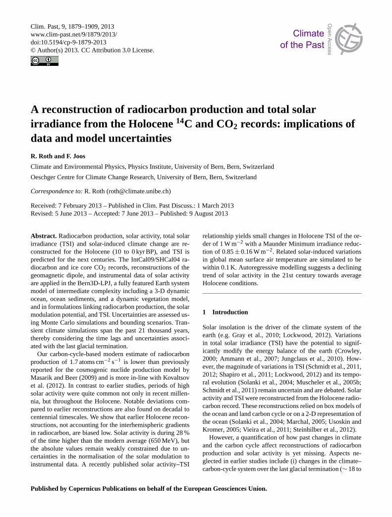
Fig. 2. (a) Reconstructed atmospheric114C of CO2 (black, left axis) and the atmospheric radiocarbon inventory (blue, right axis) overthe past 21 kyr. From 21 to 11 kyr BP, radiocarbon data are from IntCal09 (Reimer et al., 2009). Afterward, we use IntCal09 data for theNorthern Hemisphere and SHCal04 (McCormac et al., 2004) for the Southern Hemisphere, thereby taking into account the interhemisphericgradient of approximately 8 ‰ and hemisphere-specific anthropogenic depletion of14C during the industrial period. The two records are notdistinguishable in this figure because of their proximity – see(c) for a zoom-in. The atmospheric radiocarbon inventory is computed fromthe114C records and the CO2 record fromMonnin et al.(2004). (b) The 1σ error assigned to the114C record and used as input for theMonte Carlo uncertainty analysis.
to the surface ocean. These weathering input fluxes arediagnosed at the end of the sediment spin-up and kept con-stant thereafter. (iii) The coupled model is forced into a LGMstate by applying corresponding orbital settings, GHG ra-diative forcing, freshwater relocation from the ocean to theice sheets and a LGM dust influx field. Atmospheric tracegases CO2 (185 ppm),δ13C (−6.4 ‰) and114C (432 ‰) areprescribed. The model is then allowed to re-equilibrate for50 kyr.
Next, the model is integrated forward in time from21 kyr BP until 1950 AD using the following natural and an-thropogenic external forcings (Figs.2, 3 and4): atmosphericCO2 as compiled byJoos and Spahni(2008), 13CO2 (Franceyet al., 1999; Elsig et al., 2009; Schmitt et al., 2012), 114C ofCO2 (McCormac et al., 2004; Reimer et al., 2009), orbital pa-rameters (Berger, 1978), radiative forcing due to GHGs CO2,CH4 and N2O (Joos and Spahni, 2008). Iron fertilisation istaken into account by interpolating LGM (Mahowald et al.,2006) and modern dust forcing (Luo et al., 2003) following aspline-fit to the EPICA Dome C (EDC) dust record (Lambertet al., 2008). Shallow water carbonate deposition history istaken fromVecsei and Berger(2004). The ice sheet extent(including freshwater relocation and albedo changes) duringthe deglaciation is scaled between LGM and modern fieldsof Peltier (1994) using the benthicδ18O stack ofLisiecki
and Raymo(2005) which was low-pass filtered with a cutoffperiod of 10 kyr. From 850 to 1950 AD, volcanic aerosols(based onCrowley, 2000, prepared by UVic), sulfate aerosolforcing applying the method byReader and Boer(1998) de-tailed by Steinacher(2011), total solar irradiance forcingfrom PMIP3/CMIP5 (Wang et al., 2005; Delaygue and Bard,2011) and carbon emissions from fossil fuel and cement pro-duction are taken into account (Andres et al., 1999).
The land module is forced by a 31 yr monthly ClimaticResearch Unit (CRU) climatology for temperature, precipita-tion and cloud cover. On this CRU-baseline climatology, wesuperpose interpolated anomalies from snapshot simulationsperformed with the HadCM3 model (Singarayer and Valdes,2010). In addition, global mean temperature deviations withrespect to 850 AD are used to scale climate anomaly fieldsobtained from global warming simulations with the NCARAOGCM from 850 to 1950 AD applying a linear pattern scal-ing approach (Joos et al., 2001). Changes in sea level andice sheet extent influence the number and locations of gridcells available for plant growth and carbon storage; we ap-ply interpolated land masks from the ICE5G-VM2 model(Peltier, 2004). Anthropogenic land cover change duringthe Holocene is prescribed following the HYDE 3.1 dataset(Klein Goldewijk, 2001; Klein Goldewijk and van Drecht,2006).
www.clim-past.net/9/1879/2013/ Clim. Past, 9, 1879–1909, 2013

1884 R. Roth and F. Joos: A reconstruction of radiocarbon production and total solar irradiance
atmospheric CO2 [ppm] and [W/m2]
180.0200.0220.0240.0260.0280.0300.0320.0
-1.78
-0.81
0.02
0.73
N2O and CH4 radiative forcing [W/m2]
-0.4
-0.2
0.0
0.2
sea level [m]
-120.0-100.0-80.0-60.0-40.0-20.0
0.0
Coral reef build-up [MtC/yr]
0.010.020.030.040.050.0
dust deposition [0=LGM,1=modern]
0.00.20.40.60.81.0
time [yr B.P.]
idealised forcings: wind stress & α
05000100001500020000
glacial
modern
a
b
c
d
e
f
Fig. 3. Main forcings affecting the (preindustrial) Holocene carbon cycle. For completeness, the time series are shown starting from theLGM, i.e. the starting point of our transient simulations.(a) Atmospheric CO2 used both for the radiative forcing as well as for the biogeo-chemical code,(b) radiative forcing of CH4 and N2O reported as deviation from preindustrial values,(c) sea level record,(d) shallow watercarbonate deposition,(e) (smoothed and normalised) EDC dust record to interpolate between LGM and modern dust deposition fields, and(f) hypothetical wind stress/remineralisation depth exponent (α) forcings used for experiments CIRC/BIO. The reader is referred to the maintext for details and references to the individual forcing components.
In all transient simulations, the model’s atmosphereis forced with the IntCal09 (21 kyr BP to 1950 AD,Reimer et al., 2009) and SHCal04 (11 kyr BP to 1950 AD,McCormac et al., 2004) records for the Northern and South-ern Hemisphere, respectively (Fig.2a). For the equatorial re-gion (20◦ N to 20◦ S), we use the arithmetic mean of thesetwo records. Since SHCal04 does not reach as far back intime as the IntCal09 record, we use IntCal09 data for bothhemispheres before 11 kyr BP. Between the 5 yr spaced data-points given by these records, cubic interpolation is applied.
The Earth system underwent a major reorganisation dur-ing the last glacial termination as evidenced by warming,ice sheet retreat, sea level rise and an increase in CO2 andother GHGs (Shackleton, 2001; Clark et al., 2012). Mem-ory effects associated with the long lifetime of radiocarbon(8267 yr) and the long timescales involved in ocean sedi-ment interactions imply that processes during the last glacialtermination (ca. 18 to 11 kyr BP) influence the evolution ofcarbon and radiocarbon during the Holocene (Menviel andJoos, 2012). Although many hypotheses are discussed in theliterature on the mechanism governing the deglacial CO2 rise(e.g. Kohler et al., 2005; Brovkin et al., 2007; Tagliabue
et al., 2009; Bouttes et al., 2011; Menviel et al., 2012), it re-mains unclear how individual processes have quantitativelycontributed to the reconstructed changes in CO2 and14CO2over the termination. The identified processes may be distin-guished into three classes: (i) relatively well-known mech-anisms such as changes in temperature, salinity, an expan-sion of North Atlantic Deep Water, sea ice retreat, a reduc-tion in iron input and carbon accumulation on land as alsorepresented in our standard model setup; (ii) an increase indeep ocean ventilation over the termination as suggested bya range of proxy data (e.g.Franois et al., 1997; Adkins et al.,2002; Hodell et al., 2003; Galbraith et al., 2007; Andersonet al., 2009; Schmitt et al., 2012; Burke and Robinson, 2012)and modelling work (e.g.Tschumi et al., 2011); (iii) a rangeof mechanisms associated with changes in the marine biolog-ical cycling of organic carbon, calcium carbonate, and opalin addition to those included in (i).
The relatively well-known forcings implemented in ourstandard setup explain only about half of the reconstructedCO2 increase over the termination (Menviel et al., 2012).This indicates that the model misses important processes orfeedbacks concerning the cycling of carbon in the ocean. To
Clim. Past, 9, 1879–1909, 2013 www.clim-past.net/9/1879/2013/

R. Roth and F. Joos: A reconstruction of radiocarbon production and total solar irradiance 1885
atmospheric CO2 [ppm] and [W/m2]
280290300310
0.000.190.370.54
N2O and CH4 rad. forcing [W/m2]
0.00
0.10
0.20
volcanic forcing [W/m2]
-10.0-8.0-6.0-4.0-2.00.02.0
TSI [W/m2]
1364.51365.01365.51366.01366.51367.0
SO4 radiative forcing [W/m2]
-0.40-0.30-0.20-0.100.00
land-use area [1012 m2]
0.0
10.0
20.0
30.0
40.0
fossil fuel emissions [GtC/yr]
time [yr A.D.]
0.0
0.5
1.0
1.5
2.0
1000 1100 1200 1300 1400 1500 1600 1700 1800 1900
a
b
c
d
e
f
g
Fig. 4. Forcings for the last millennium including the industrial period:(a) atmospheric CO2 used both for the radiative forcing as well asfor the biogeochemical code,(b) radiative forcing of CH4 and N2O reported as deviation from preindustrial values,(c) volcanic forcing,(d) solar forcing,(e) SO4 radiative forcing,(f) anthropogenic land-use area and(g) carbon emissions from fossil fuel use (including cementproduction). The reader is referred to the main text for details and references to the individual forcing components.
this end, we apply two idealised scenarios for this missingmechanism, regarded as bounding cases in terms of theirimpacts on atmospheric114C. In the first scenario, termedCIRC, the atmospheric carbon budget over the terminationis approximately closed by forcing changes in deep oceanventilation. In the second, termed BIO, the carbon budgetis closed by imposing changes in the biological cycling ofcarbon.
14C in the atmosphere and the deep ocean is sensitive tothe surface-to-deep transport of14C. This 14C transport isdominated by physical transport (advection, diffusion, con-vection), whereas biological fluxes play a small role. Con-sequently, processes reducing the thermohaline circulation(THC), the surface-to-deep transport rate, and deep oceanventilation tend to increase114C of atmospheric CO2 andto decrease114C of DIC in the deep. Recently, a range ofobservational studies addressed deglacial changes in radio-carbon and deep ocean ventilation. Some authors report ex-tremely high ventilation ages up to 5000 yr (Marchitto et al.,2007; Bryan et al., 2010; Skinner et al., 2010; Thornalleyet al., 2011), while others find no evidence for such an oldabyssal water mass (De Pol-Holz et al., 2010). In contrast,changes in processes related to the biologic cycle of carbon
such as changes in export production or the remineralisa-tion of organic carbon hardly affect114C of DIC and CO2,despite their potentially strong impact on atmospheric CO2(e.g.Tschumi et al., 2011).
Technically, these two bounding cases are realised as fol-lows. In the experiment BIO, we imply (in addition to allother forcings) a change in the depth where exported par-ticulate organic matter is remineralised; the exponent (α) inthe power law describing the vertical POM flux profile (Mar-tin curve) is increased during the termination from a lowglacial value (Fig.3f). A decrease in the average remineral-isation depth over the termination leads to an increase in at-mospheric CO2 (Matsumoto, 2007; Kwon et al., 2009; Men-viel et al., 2012), but does not substantially affect114C. α
is increased from 0.8 to 1.0 during the termination in BIO,while in the other experimentsα is set to 0.9. In the ex-periment CIRC, ocean circulation is strongly reduced at theLGM by reducing the wind stress globally by 50 % relativeto modern values. The wind stress is then linearly relaxed tomodern values over the termination (18 to 11 kyr BP, Fig.3f).This leads to a transfer of old carbon from the deep oceanto the atmosphere, raising atmospheric CO2 and lowering114C of CO2 (Tschumi et al., 2011). We stress that changes
www.clim-past.net/9/1879/2013/ Clim. Past, 9, 1879–1909, 2013

1886 R. Roth and F. Joos: A reconstruction of radiocarbon production and total solar irradiance
in wind stress and remineralisation depth are used here astuning knobs and not considered as realistic.
To further assess the sensitivity of the diagnosed radio-carbon production on the cycling of carbon and climate, weperform a control simulation (CTL) where all forcings ex-cept atmospheric CO2 (and isotopes) are kept constant at PIvalues. This setup corresponds to earlier box model studieswhere the Holocene climate was assumed to be constant.
As noted, the transient evolution of atmospheric CO2 and114C over the glacial termination is prescribed in all threesetups (CTL, CIRC, BIO). Thus, the influence of changingconditions over the last glacial termination on Holocene14Cdynamics is taken into account, at least to a first order, ineach of the three setups.
2.3 The production rate of radiocarbon,Q
The14C production rateQ is diagnosed by solving the atmo-spheric14C budget equation in the model. The model calcu-lates the net fluxes from the atmosphere to the land biosphere(14Fab) and to the ocean (14Fas) under prescribed14CO2 fora given carbon-cycle/climate state. Equivalently, the changesin 14C inventory and14C decay of individual land and oceancarbon reservoirs are computed. Data-based estimates for theocean and land inventory are used to match preindustrial ra-diocarbon inventories as closely as possible. The productionrate is then given at any timet by:
Q(t) =Iatm,data(t)
τ+
dIatm,data(t)
dt+
14Fbudget(t)
+Iocn,model(t)
τ+
dIocn,model(t)
dt+
1Iocn,data-model(t = t0)
τ
+Ised,model(t)
τ+
dIsed,model(t)
dt+
14Fburial(t)
}=
14Fas
+Ilnd,model(t)
τ+
dIlnd,model(t)
dt+
1Ilnd,data-model(t = t0)
τ=
14Fab. (1)
Here, I and F denote14C inventories and fluxes, andτ(8267 yr) is the mean14C lifetime with respect to radioac-tive decay. Subscripts atm, ocn, sed, and lnd refer to the at-mosphere, the ocean, reactive ocean sediments, and the landbiosphere, respectively. Subscript data indicates that termsare prescribed from reconstructions and subscript modelthat values are calculated with the model.14Fburial is thenet loss of14C associated with the weathering/burial car-bon fluxes.1Iocn,data-model(t = t0) represents a (constant)correction, defined as the difference between the modelledand observation-based inventory of DI14C in the oceanplus an estimate of the14C inventory associated with re-fractory DOM not represented in our model. In analogue,1Ilnd,data-model(t = t0) denotes a constant14C decay rate as-sociated with terrestrial carbon pools not simulated in ourmodel.14Fbudget is a correction associated with the carbonflux diagnosed to close remaining imbalances in the atmo-spheric CO2 budget.
2.3.1 Observation-based versus simulated oceanradiocarbon inventory
The global ocean inorganic radiocarbon inventory is esti-mated using the gridded data provided by GLODAP for thepreindustrial state (Key et al., 2004) and in situ density cal-culated from World Ocean Atlas 2009 (WOA09) temper-ature and salinity fields (Antonov et al., 2010; Locarniniet al., 2010). Since the entire ocean is not covered by theGLODAP data, we fill these gaps by assuming the globalmean14C concentration in these regions (e.g. in the Arc-tic Ocean). The result of this exercise is 3.27× 10⁶ molof DI14C. Hansell et al.(2009) estimated a global refrac-tory DOC inventory of 624 Gt C.114C of DOC measure-ments are rare, but data in the central North Pacific (Baueret al., 1992) suggest high radiocarbon ages of∼ 6000 yr,corresponding to a114C value of∼ −530 ‰. Taking thisvalue as representative yields an additional 2.9× 10⁴ mol14C. The preindustrial14C inventory associated with labileDOM is estimated from our model results to be 1.3× 10³ mol14C. This yields a data-based radiocarbon inventory asso-ciated with DIC and labile and refractory DOM in theocean of 3.30× 10⁶ mol. The corresponding preindustrialmodelled ocean inventory yields 3.05× 10⁶ mol for BIO,3.32× 106 mol for CIRC and 3.10× 10⁶ mol for CTL. Thus,the correction1Iocn,data-model(t = t0) is less than 8 % in thecase of BIO and less than 1 % for CIRC and CTL.
2.3.2 Observation-based versus simulated terrestrialradiocarbon inventory
As our model for the terrestrial biosphere does not includecarbon stored as peatlands and permafrost soils. We estimatethis pool to contain approximately 1000 Gt C of old carbonwith a isotopic signature of−400 ‰ (thus roughly one half-life old). Although small compared to the uncertainty in theoceanic inventory, we include these 5.9× 10⁴ mol of 14C inour budget as a constant correction1Ilnd,data-model(t = t0).
2.3.3 Closing the atmospheric CO2 budget
The atmospheric carbon budget is closed in the transient sim-ulations by diagnosing an additional carbon fluxFbudget:
Fbudget= −dNatm,data
dt− E + Fas + Fab (2)
where the change in the atmospheric carbon inventory(dNatm/dt) is prescribed from ice core data,E are fossil fuelcarbon emissions, andFas andFab the net carbon fluxes intothe ocean and the land biosphere. The magnitude of this in-ferred emission indicates the discrepancy between modelledand ice core CO2 and provides a measure of how well themodel is able to simulate the reconstructed CO2 evolution.We assign to this flux (of unknown origin) a114C equal thecontemporary atmosphere and an associated uncertainty in
Clim. Past, 9, 1879–1909, 2013 www.clim-past.net/9/1879/2013/

R. Roth and F. Joos: A reconstruction of radiocarbon production and total solar irradiance 1887
114C of ±200 ‰. This is not critical asFbudgetand associ-ated uncertainties in the14C budget are generally small overthe Holocene for simulations CIRC and BIO (see AppendixFig. A1e).
The production rate is either reported as mol yr−1 or al-ternatively atoms cm−2 s−1. The atmospheric area is set to5.10× 1014 m2 in our model, therefore the two quantities arerelated as 1 atom cm−2 s−1 = 267.0 mol yr−1.
2.4 Solar activity
Radiocarbon, as other cosmogenic radionuclides, are primar-ily produced at high latitudes of earth’s upper atmospheredue to nuclear reactions induced by high-energy galactic cos-mic rays (GCR). Far away from the solar system, this flux isto a good approximation constant in time, but the intensityreaching the earth is modulated by two mechanism: (i) theshielding effect of the geomagnetic dipole field and (ii) themodulation due to the magnetic field enclosed in the so-lar wind. By knowing the past history of the geomagneticdipole moment and the production rate of radionuclides, the“strength” of solar activity can therefore be calculated.
The sun’s activity is parametrised by a scalar parameter inthe force field approximation, the so-called solar modulationpotential8 (Gleeson and Axford, 1968). This parameter de-scribes the modulation of the local interstellar spectrum (LIS)at 1 AU. A high solar activity (i.e. a high value of8) leadsto a stronger magnetic shielding of GCR and thus lowers theproduction rate of cosmogenic radionuclides. Similarly, theproduction rate decreases with a higher geomagnetic shield-ing, expressed as the virtual axis dipole moment (VADM).
The calculation of the normalised (relative to modern)Q
for a given VADM and8 is based on particle simulationsperformed byMasarik and Beer(1999). This is the stan-dard approach to convert cosmogenic radionuclide produc-tion rates into solar activity as applied byMuscheler et al.(2007), Steinhilber et al.(2008) andSteinhilber et al.(2012),but differs from the model to reconstruct TSI recently usedby Vieira et al.(2011).
The GCR flux entering the solar system is assumed toremain constant within this approach, even thoughMiyakeet al. (2012) found recently evidence for a short-term spikein annual114C. The cause of this spike (Hambaryan andNeuhauser, 2013; Usoskin et al., 2013) is currently debatedin the literature.
At the time of writing, three reconstructions of the pastgeomagnetic field are available to us spanning the past10 kyr (Yang et al., 2000; Knudsen et al., 2008; Korte et al.,2011), shown in Fig.11 together with the VADM value of8.22× 1022 Am−2 for the period 1840–1990 estimated byJackson et al.(2000). The reconstructions byYang et al.(2000) andKnudsen et al.(2008), relying both on the samedatabase (GEOMAGIA 50), were extensively used in thepast for solar activity reconstructions (Muscheler et al., 2007;Steinhilber et al., 2008; Vieira et al., 2011; Steinhilber et al.,
2012). We use the most recently published reconstruction byKorte et al.(2011) for our calculations.
For conversion from8 into TSI, we follow the procedureoutlined inSteinhilber et al.(2009); Steinhilber et al.(2010)which consists of two individual steps. First, the radial com-ponent of the interplanetary magnetic field,Br, is expressedas a function of8:
|Br(t)| = 0.56BIMF,0 ×
(8(t)vSW,0
80vSW(t)
)1/α
×
[1 +
(RSEω cos9
vSW(t)
)2]−
12
, (3)
where vSW is the (time-dependent) solar wind speed(Steinhilber et al., 2010); BIMF,0, 80, vSW,0are normalisationfactors;RSE is the mean Sun–Earth distance;ω the angularsolar rotation rate; and9 the heliographic latitude. The fac-tor 0.56 has been introduced to adjust the field obtained fromthe Parker theory with observations. The exponent is set tobe in the rangeα = 1.7± 0.3 as inSteinhilber et al.(2009).
Second, theBr–TSI relationship derived byFrohlich(2009) is used to calculate the total solar irradiance:
TSI = (1364.64 ± 0.40)Wm−2+ Br · (0.38 ± 0.17)Wm−2nT−1. (4)
This model of convertingBr (here in units of nanotesla) intoTSI is not physically based, but results from a fit to observa-tions for the relatively short epoch where high-quality obser-vational data is available. Note that theBr–TSI relationshipis only valid for solar cycle minima, therefore an artificial si-nusoidal solar cycle (with zero mean) has to be added to the(solar-cycle averaged)8 before applying Eqs. (3) and (4). Inthe results section, we show for simplicity solar cycle aver-ages (i.e. without the artificial 11 yr solar cycle).
A point to stress is that the amplitude of low-frequencyTSI variations is limited by Eq. (4) and small. This is a con-sequence of the assumption underlying Eq. (4) that recentsatellite data, which show a limited decadal-scale variabil-ity in TSI, can be extrapolated to past centuries and millen-nia. Small long-term variations in TSI are in agreement witha range of recent reconstructions (Schmidt et al., 2011), butin conflict withShapiro et al.(2011), who report much largerTSI variations.
3 Results
3.1 Sensitivity experiments
We start the discussion by analysing the response of theBern3D-LPJ model to regular sinusoidal changes in the at-mospheric radiocarbon ratio. The theoretical background isthat any time series can be translated into its power spec-trum using Fourier transformation. Thus, the response ofthe model to perturbations with different frequencies char-acterises the model for a given state (climate, CO2, land-use
www.clim-past.net/9/1879/2013/ Clim. Past, 9, 1879–1909, 2013

1888 R. Roth and F. Joos: A reconstruction of radiocarbon production and total solar irradiance
area, etc.). The experimental setup for this sensitivity sim-ulation is as follows.114C is varied according to a sinewave with an amplitude of 10 ‰ and distinct period. Thesine wave is repeated until the model response is at equi-librium. Periods between 5 and 1000 yr are selected. Atmo-spheric CO2 (278 ppm), climate and all other boundary con-ditions are kept fixed at preindustrial values. The natural car-bon cycle acts like a smoothing filter and changes in atmo-spheric114C arising from variations inQ are attenuated anddelayed (Fig.5a). That is the relative variations in114C aresmaller than the relative variations inQ. Here, we are in-terested in inverting this natural process and diagnosingQ
from reconstructed variations in radiocarbon. Consequently,we analyse not the attenuation of the radiocarbon signal, butthe amplification ofQ for a given variation in atmosphericradiocarbon. Figure5a shows the amplification inQ, definedas the relative change inQ divided by the relative change inthe radiocarbon to carbon ratio,14R. For example, an am-plification of 10 means that if14R oscillates by 1 %, thenQoscillates by 10 % around its mean value. The amplificationis largest for high-frequency variations and decreases fromabove 100 for a period of 5 yr to around 10 for a period of1000 yr and to 2 for a period of 10 000 yr. High-frequencyvariations in the14C reconstruction arising from uncertain-ties in the radiocarbon measurements may thus translate intosignificant uncertainties inQ. We will address this problemin the following sections by applying a Monte Carlo proce-dure to vary114C measurements within their uncertainties(see Appendix A1).
The atmospheric radiocarbon anomaly induced by varia-tion in production is partly mitigated through radiocarbonuptake by the ocean and the land. The relative importanceof land versus ocean uptake of the perturbation dependsstrongly on the timescale of the perturbation (Fig.5b). Forannual- to decadal-scale perturbations, the ocean and the landuptake are roughly of equal importance. This can be under-stood by considering that the net primary productivity onland (60 Gt C per year) is of similar magnitude as the grossair-to-sea flux of CO2 (57 Gt C per year) into the ocean. Thus,these fluxes carry approximately the same amount of radio-carbon away from the atmosphere. On the other hand, if theperturbation in production is varying slower than the typ-ical overturning timescales of the ocean and the land bio-sphere, then the radiocarbon perturbation in the ratio is dis-tributed roughly proportional to the carbon inventory of thedifferent reservoirs (or to the steady-state radiocarbon flux tothe ocean and the land, i.e. 430 vs. 29.1 mol yr−1). Conse-quently, the ratio between the14C flux anomalies into oceanand land,1Fas: 1Fab (with respect to an unperturbed state),is the higher the lower frequency of the applied perturbation(Fig. 5b). Note that these results are largely independent ofthe magnitude in the applied114C variations; we run theseexperiments with amplitudes of±10 and±100 ‰. Assum-ing a constant carbon cycle and climate,Q can be calculated
a
period [years]
Δ14
Fas/Δ14
Fab
0
1
2
3
4
5
6
7
10 100 1000 10000
(ΔQ
/Q0)
/ (Δ
14R
/14R
0)
ph
ase
[d
eg
]
10
100
-80
-70
-60
-50
-40
-30
10 100 1000 10000
b
Fig. 5. Response of the Bern3D-LPJ model to periodic sinusoidalvariations in the atmospheric radiocarbon ratio (14R) with an ampli-tude of 10 ‰ (in units of114C). (a) Relative change in productionrate,Q, divided by the relative change in14R (with respect to a PIsteady state; black) and the phase shift betweenQ and14R (red, leftaxis); Q is always leading atmospheric14R. (b) Relative changesin the net atmosphere-to-sea (Fas) and the net atmosphere-to-landbiosphere (Fab) fluxes of14C for the same simulations.
by replacing the carbon-cycle–climate model by the model-derived Fourier filter (Fig.5a) (Usoskin and Kromer, 2005).
Preindustrial carbon and radiocarbon inventories
The loss of14C is driven by the radioactive decay flux in thedifferent reservoirs. The base level of this flux is proportionalto the14C inventory and a reasonable representation of theseinventories is thus a prerequisite to estimate14C productionrates. In the following, modelled and observation-based car-bon and radiocarbon inventories before the onset of industri-alisation are compared (Table1) and briefly discussed.
The atmospheric14C inventory is given by the CO2 and114C input data and therefore fully determined by the forc-ing and their uncertainty. The ocean model represents theobservation-based estimate of the global ocean14C inven-tory within 1 % for the setup CIRC and within 8 % for thesetup BIO. These deviations are within the uncertainty of theobservational data. Nevertheless, this offset is corrected forwhenQ is calculated (see Eq. 1).
The model is also able to represent the observation-basedspatial distribution of14C in the ocean (Fig.7). Both observa-tion and model results show the highest14C concentrations inthe thermocline of the Atlantic Ocean and the lowest concen-trations in the deep North Pacific. Deviations between mod-elled and reconstructed concentrations are less than 5 % andtypically less than 2 %. The model shows in general too-high
Clim. Past, 9, 1879–1909, 2013 www.clim-past.net/9/1879/2013/

R. Roth and F. Joos: A reconstruction of radiocarbon production and total solar irradiance 1889
Table 1.Preindustrial model versus data-based carbon and14C in-ventory estimates. The model-based oceanic inventories are calcu-lated as the average of the experiments BIO and CIRC.
Bern3D-LPJ Data
Carbon 14C Carbon 14C[Gt C] [105 mol] [Gt C] [105 mol]
ATM 593 0.591 593a 0.591b
LND 1930 1.79 2500–3500c
OCN 38 070 32.0 38 200d 33.00d
Carbon 14C Carbon 14C[Gt C yr−1
] [mol yr−1] [Gt C yr−1
] [mol yr−1]
SED 0.501 52 0.22–0.4e
a MacFarling Meure et al.(2006); b McCormac et al.(2004); Reimer et al.(2009); c Watson(2000); Tarnocai et al.(2009); Yu et al.(2010); d Key et al.(2004); Hansell et al.(2009); e Sarmiento and Gruber(2006); Feely et al.(2004).
radiocarbon concentrations in the upper 1000 m, while theconcentration is lower than indicated by the GLODAP dataat depth.
Modelled loss of radiocarbon by sedimentary processes,namely burial of POM and CaCO3 into the diageneticallyconsolidated zone and particle and dissolution fluxes from/tothe ocean, accounts for 52 mol yr−1 (or roughly 11 % of thetotal 14C sink). This model estimate may be on the high sideas the ocean-to-sediment net flux in the Bern3D-LPJ modelof 0.5 Gt C yr−1 is slightly higher than independent estimatesin the range of 0.2 to 0.4 Gt C yr−1.
The total simulated carbon stored in living biomassand soils is 1930 Gt C. As discussed above, this is order1000 Gt C lower than best estimates, mainly because peat andpermafrost dynamics (Yu et al., 2010; Spahni et al., 2012)are not explicitly simulated in the LPJ version applied here.The model–data discrepancy in carbon is less than 3 % ofthe total carbon inventory in ocean, land, and atmosphere. Ittranslates into 5.9× 10⁵ mol of 14C when assuming a114Cof −400 ‰ for this old biomass. This is well within the un-certainty range of the total14C inventory.
3.2 Transient results for the carbon budget and deepocean ventilation
Next, we discuss how global mean temperature, deep oceanventilation, and the carbon budget evolved over the past21 kyr in our two bounding simulations (CIRC and BIO).Global average surface air temperature (SAT, Fig.6a) andsea surface temperature (SST, not shown) are simulated to in-crease by∼ 0.8◦C over the Holocene. In experiment CIRC,the global energy balance over the termination is strongly in-fluenced by the enforced change in wind stress and the sim-ulated deglacial increase in SAT is almost twice as large inexperiment CIRC than in BIO. This is a consequence of a
much larger sea ice cover and a higher planetary albedo atLGM in experiment CIRC than BIO. Circulation is slow un-der the prescribed low glacial wind stress and less heat istransported to high latitudes and less ice is exported fromthe Southern Ocean to lower latitudes in CIRC than BIO. Inother words, the sea-ice–albedo feedback is much larger inCIRC than BIO.
Deep ocean ventilation evolves very differently in CIRCthan in BIO (Fig.6b). Here, we analyse the global aver-age 14C age difference of the deep ocean (i.e. waters be-low 2000 m depth) relative to the overlying surface ocean.The surface-to-deep age difference is recorded in ocean sedi-ments as14C age offset between shells of benthic and plank-tonic (B-P) species. Results from the CTL experiment withtime-invariant ocean ventilation show that this “proxy” is notan ideal age tracer; the B-P age difference is additionally in-fluenced by transient atmospheric114C changes and variesbetween 600 and 1100 yr in CTL.
The wind-stress forcing applied in experiment CIRC leadsto an almost complete shutdown of the THC during the LGMand a recovery to Holocene values over the termination. Sim-ulated B-P age increases from 2000 yr at LGM to peak at2900 yr by 16.5 kyr BP. A slight and after 12 kyr BP a morepronounced decrease follows to the late Holocene B-P age ofabout 1000 yr. B-P variations are much smaller in simulationBIO, as no changes in wind stress are applied; B-P age variesbetween 1000 and 1700 yr.
1114C, i.e. the global mean difference in114C betweenthe deep ocean and the atmosphere is−500 ‰ in CIRC un-til Heinrich Stadial 1 (HS1) (−350 ‰ in BIO), followed bya sharp increase of approximately 150–200 ‰ and a slowrelaxation to late-Holocene values (∼ −170 ‰). This be-haviour is also present in recently analysed sediment cores,see e.g.Burke and Robinson(2012) and references therein.The sharp increase in1114C following HS1 is mainlydriven by the prescribed fast atmospheric drop (Broecker andBarker, 2007).
The forcings prescribed in our bounding experimentsCIRC and BIO are broadly sufficient to reproduce the re-constructed deglacial CO2 increase. This is evidenced by ananalysis of the atmospheric carbon budget (Fig.6d and f).In the control simulation (CTL) an addition of 1700 Gt C isrequired to close the budget. In contrast, the mismatch inthe budget is close to zero for BIO and about−100 Gt C forCIRC at the end of the simulation. In other words, only smallemissions from unknown origin have to be applied on aver-age to close the budget. Both experiments need a CO2 sinkin the early Holocene as indicated by the negative missingemissions. Such a sink could have been the carbon uptake ofNorthern Hemisphere peatlands (Yu et al., 2010), as peatlanddynamics are not included in this model version. In summary,simulation CIRC corresponds to the picture of a slowly ven-tilated ocean during the LGM, whereas deep ocean ventila-tion changes remain small in BIO and are absent in the CTLsimulation. The atmospheric carbon budget is approximately
www.clim-past.net/9/1879/2013/ Clim. Past, 9, 1879–1909, 2013
1890 R. Roth and F. Joos: A reconstruction of radiocarbon production and total solar irradiance
13.3
13.9
14.5
missing CO2-flux [GtC/yr]
1000 1100 1200 1300 1400 1500 1600 1700 1800 1900
-1.0
0.0
1.0
time [yr B.P.]
time [yr A.D.]
BIOCIRC
CTL
3.06.09.0
12.015.0
0.51.01.52.02.53.0
-1.0-0.50.00.51.0
05000100001500020000050010001500
initialisation
deep ocean B-Pventilation age [kyr]
missing CO2-flux [GtC/yr]
cumulative missingCO2 flux [GtC]
SAT [oC]
SAT [oC]
a
b
c
d
e
f
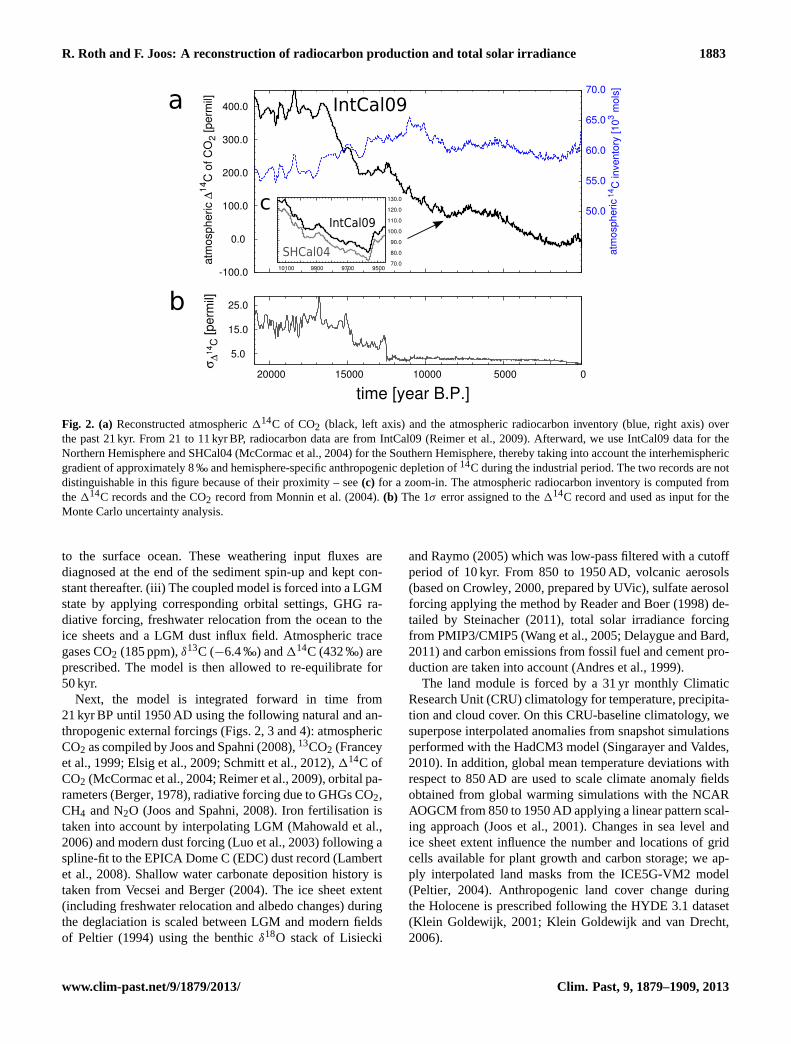
Fig. 6. Transient model response during the past 21 kyr of(a) global mean surface air temperature (SAT),(b) globally averaged benthic-planktonic (surface-deep) reservoir age calculated as14C age offset from the global ocean below 2000 m relative to the surface ocean,(c) implied carbon flux to solve the atmospheric budget (Fbudget) and(d) cumulative sum thereof for the experiments BIO, CIRC and thecontrol run CTL. For the last millennium, SAT andFbudgetis shown in detail in the lower two panels(e, f). The grey shaded area indicatesthe period used to initialise the model. The radiocarbon production rate is diagnosed only for the last 10 kyr.
closed in simulations CIRC and BIO, whereas a substantialexternal carbon input is required in simulation CTL. Thesethree simulations provide thus three radically different evo-lutions of the carbon cycle over the past 21 kyr and will serveus to assess uncertainties in inferred radiocarbon productionrates due to our incomplete understanding of the past carboncycle.
3.2.1 Time evolution of the radiocarbon production rate
Total inferred radiocarbon production,Q, varies between350 and 650 mol yr−1 during the Holocene (Fig.8d). Vari-ations on multi-decadal to centennial timescales are typi-cally within 100 mol yr−1. The differences inQ in the earlyHolocene between the model setups CIRC, BIO, and CTLare mainly explained by offsets in the absolute value ofQ,while the timing and magnitude of multi-decadal to centen-nial variations are very similar for the three setups. The ab-solute value ofQ is about 40 mol yr−1 higher in CIRC thanin BIO and about 60 mol yr−1 higher in CIRC than in CTL
at 10 kyr BP. This difference becomes very small in the lateHolocene and results are almost identical for CIRC and BIOafter 4 kyr BP. Note that the absolute (preindustrial) value ofthe production rate is equal in all three setups per definition(see Eq. 1).
The inferredQ is assigned according to Eq. (1) to individ-ual contributions from a net14C flux from the atmosphere tothe ocean (14Fas), a net flux to the land (14Fab), and atmo-spheric loss terms (Fig.8). Variations in these three termscontribute about equally to variations inQ on decadal tocentennial timescales, whereas millennial-scale variations inQ are almost entirely attributed to changes in14Fas. This isin agreement with the results from the Fourier analysis pre-sented in Sect. 3.1. Holocene and preindustrial mean fluxesand their temporal variance are listed in Table2.
The oceanic component entering the calculation ofQ isthreefold (Fig.9): (i) the compensation of the DI14C (and asmall contribution of DO14C) decay proportional to its in-ventory, (ii) changes in the inventory of14C itself mainlydriven byFas and (iii) the export, rain and subsequent burial
Clim. Past, 9, 1879–1909, 2013 www.clim-past.net/9/1879/2013/

R. Roth and F. Joos: A reconstruction of radiocarbon production and total solar irradiance 1891
model
data
model -data
DI14C [μmol/l/14RSTD]
N
N
Fig. 7.Comparison of modern modelled and data-based (GLODAP,WOA09) oceanic distribution of14C in its dominant form of dissolved in-organic carbon (DI14C) along a transect through the Atlantic, Southern Ocean and Pacific. The lowest panel shows the model–data difference.
Table 2. The atmospheric radiocarbon budget (positive numbers:loss of 14C) averaged over the last 10 kyr and for preindustrialtimes (1750–1900 AD). The statistical uncertainty becomes negli-gible due to the averaging over hundreds of datapoints and is notgiven here. Instead, we report
√VAR (where VAR is the variance
in time) to quantify the temporal variability of the correspondingfluxes. The bulk uncertainty in the time-averaged fluxes can be es-timated by the uncertainty in the corresponding radiocarbon reser-voirs and is of the order of 15 % (1σ ), except for the atmosphericcomponent which is tightly constrained by data.
Holocene (10–0 kyr BP) Preindustrial (1750–1900 AD)
14C loss Best guess√
VAR Best guess√
VAR[mol yr−1
]
14Fas 436 27 451 3314Fab 25 25 −6.9 47ATM 11 23 24 44
Total 472 57 468 35
of Ca14CO3 and PO14C. Thus, the mentioned offset in14Fasbetween CIRC and BIO at the early Holocene are the resultof differences in the dynamical evolution of the whole-oceanDIC inventories and its114C signature. During LGM condi-tions, the oceanic14C inventory is larger for BIO than CIRCas the deep ocean is more depleted in the slowly overturn-ing ocean of setup CIRC. Accordingly the decay of14C and14Fas is higher in simulation BIO than in CIRC (Fig.9). Thesimulated oceanic14C inventory decreases both in CIRC andBIO as the (prescribed) atmospheric114C decreases. How-ever, this decrease is smaller in CIRC than in BIO as the en-forced increase in the THC and in ocean ventilation in CIRCleads to an additional14C flux into the ocean. In addition,the strengthened ventilation leads to a peak in organic matterexport and burial while the reduced remineralisation depthin BIO leads to the opposite effect (as less POM is reach-ing the seafloor). In total, the higher oceanic radiocarbon de-cay in BIO is overcompensated by the (negative) change ofthe oceanic inventory. Enhanced sedimentary loss of14C inCIRC further increases the offset, finally leading to a higherQ at 10 kyr BP of∼ 40 mol yr−1 in CIRC than in BIO. This
www.clim-past.net/9/1879/2013/ Clim. Past, 9, 1879–1909, 2013

1892 R. Roth and F. Joos: A reconstruction of radiocarbon production and total solar irradiance
aCTLCIRC BIO
-100.0
-50.0
0.0
50.0
100.0
-100.0
-50.0
0.0
50.0
100.0
time [year B.P.]0200040006000800010000
400.0450.0500.0550.0600.0650.0
time [year A.D.]
INT09
CTL CIRC BIO350.0
400.0
450.0
500.0
550.0
600.0
1000 1100 1200 1300 1400 1500 1600 1700 1800 1900
atmosphere
total
units: [mol/yr]
360.0390.0420.0450.0480.0510.0540.0
14abF
F14as
total
b
c
d
e
Fig. 8. Holocene14C fluxes in mol14C yr−1 for the different experiments:(a) changes and decay of the atmospheric inventory (includingFbudget), (b) air–biosphere flux (Fab), (c) air–sea flux (Fas) and (d) the sum of these contributions yielding the total production rateQ.(e)shows the last 1000 yr in greater detail together with an experiment (INT09) where the entire globe is forced with the Northern Hemispheredataset IntCal09 (dashed line), thereby neglecting the interhemispheric gradient in114C. Note that the time series shown in(a) and(b) havebeen smoothed with a cutoff of 40 yr (only for the visualisation) while(c)–(e)show 20 yr smoothed data as described in the main text.
offset has vanished almost completely at 7 kyr BP, apart froma small contribution from sedimentary processes.
In general, the influence of climate induced carbon cyclechanges is modest in the Holocene. This is indicated by thevery similarQ in the CTL experiment. The biggest discrep-ancy between results from CTL versus those from CIRC andBIO emerge during the industrial period.Q drops rapidlyin CTL as the combustion of the radiocarbon-depleted fos-sil fuel is not explicitly included.
In a further sensitivity run, the influence of the interhemi-spheric114C gradient onQ is explored (Fig.8e; dashedline). In simulation INT09 the Northern Hemisphere datasetIntCal09 is applied globally and all other forcings are as in
BIO. Differences inQ between CIRC/BIO and INT09 aregenerally smaller than 20 mol yr−1, but grow to 50 mol yr−1
from 1900 to 1950 AD. The reason is the different slopes inthe last decades of the Northern and Southern Hemisphererecords. This mid-20th century difference has important con-sequences for the reconstruction of solar modulation as de-scribed in Sect. 3.3. This sensitivity experiment demonstratesthat spatial gradients in atmospheric114C and in resultingradiocarbon fluxes should be taken into account, at least forthe industrial period.
In conclusion, inferred Holocene values ofQ and in par-ticular decadal to centennial variation inQ are only weaklysensitive to the details of the carbon cycle evolution over the
Clim. Past, 9, 1879–1909, 2013 www.clim-past.net/9/1879/2013/

R. Roth and F. Joos: A reconstruction of radiocarbon production and total solar irradiance 1893
BIO
420.0
440.0
460.0
480.0
-150.0-100.0-50.0
0.050.0
100.0
50.0
60.0
70.0
80.0
40005000600070008000900010000110001200013000350.0400.0450.0500.0550.0600.0650.0
units: [mol/yr]initialisation
change in 14C inventory
sedimentary processes
time [year B.P.]
total
14C decay
CIRCa
b
c
d
Fig. 9.The oceanic14C budget for the experiments BIO and CIRC for the period 13 to 4 kyr BP.(a) Decay of the data-normalised inventoryof 14C in the form of inorganic and organic carbon,(b) changes in whole ocean radiocarbon inventory, and(c) contribution from sediments(burial flux and decay of14C within the active sediment layer).(d) After 4 kyr BP, the two experiments do not show significant differencesin the total ocean and sediment14C loss.
glacial termination. On the other hand spatial gradients in at-mospheric114C and carbon emissions from fossil fuel burn-ing should be explicitly included to estimate radiocarbon pro-duction in the industrial period. In the following, we will usethe arithmetic mean of BIO and CIRC as our best estimatefor Q (Fig. 10). The final record is filtered using smoothingsplines (Enting, 1987) with a cutoff period of 20 yr in orderto remove high-frequency noise.
Total ±1 standard deviation (1σ ) uncertainties inQ
(Fig. 10, grey band) are estimated to be around 6 % at10 kyr BP and to slowly diminish to around±1–2 % by1800 AD (Appendix Fig. A1f). Overall uncertainty inQ in-creases over the industrial period and is estimated to be± 6 % by 1950 AD. The difference inQ between BIO andCIRC is assumed to reflect the uncertainty range due to ourincomplete understanding of the deglacial CO2 evolution.Uncertainties in the114C input data, the air–sea gas ex-change rate and the gross primary production (GPP) of theland biosphere are taken into account using a Monte Carloapproach and based on further sensitivity simulations (seeSect.A1 for details of the error estimation).
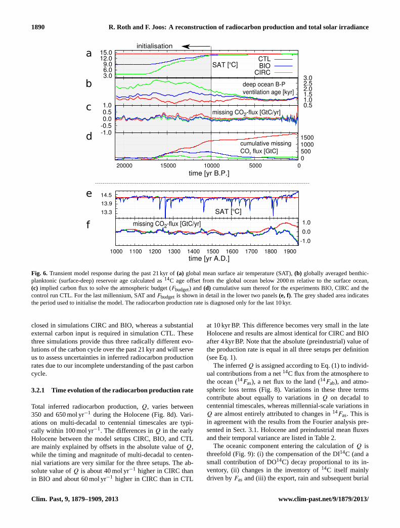
The radiocarbon production records fromUsoskin andKromer (2005) and from the Marmod09 box model (http://www.radiocarbon.org/IntCal09%20files/marmod09.csv;model described inHughen et al., 2004) show similarvariations on timescales of decades to millennia (Fig.10).
These include maxima inQ during the well-documentedsolar minima of the last millennium, generally low pro-duction, pointing to high solar activity during the Romanperiod, as well as a broad maximum around 7.5 kyr BP.However, the production estimates ofUsoskin and Kromer(2005) and Marmod09 are about 10 % lower during theentire Holocene and are in general outside our uncertaintyrange. If we can rely on our data-based estimates of thetotal radiocarbon inventory in the Earth system, then thelower average production rate in theUsoskin and Kromer(2005) and Marmod09 records suggest that the radiocarboninventory is underestimated in their setups.
In the industrial period, the Marmod09 production rate dis-plays a drop inQ by almost a factor of two. This recon-struction is intended to provide the surface age of the oceanfor the Holocene for calibration of marine samples from thattime period. Data after 1850 AD are not to be considered asthe authors purposely do not include a fossil fuel correction.Similarly, Usoskin and Kromer(2005) do not provide dataafter 1900 AD.
3.2.2 A reference radiocarbon production rate
Next, we discuss the absolute value ofQ in more detail.Averaged over the Holocene, our simulations yield a14Cproduction ofQ = 472 mol yr−1 (1.77 atoms cm−2 s−1), aslisted in Table2. Independent calculations of particle fluxes
www.clim-past.net/9/1879/2013/ Clim. Past, 9, 1879–1909, 2013
1894 R. Roth and F. Joos: A reconstruction of radiocarbon production and total solar irradiance
a
b
c
mol/y
r
ato
ms/c
m2/s
time [yr B.P.]
250
300
350
400
450
500
550
600
650
5000600070008000900010000
1
1.2
1.4
1.6
1.8
2
2.2
2.4
mol/y
r
ato
ms/
cm2/s
time [yr B.P.]
250
300
350
400
450
500
550
600
650
010002000300040005000
1
1.2
1.4
1.6
1.8
2
2.2
2.4
mol/y
r
ato
ms/
cm2/s
time [yr A.D.]
250
300
350
400
450
500
550
600
650
1000 1100 1200 1300 1400 1500 1600 1700 1800 1900
1
1.2
1.4
1.6
1.8
2
2.2
2.4
Marmod09 US05
Marmod09 US05this study
this study
Fig. 10. (a, b)Total14C production rate from this study (black line with grey 1σ shading) and the reconstructions fromUsoskin and Kromer(2005) (blue) and the output of the Marmod09 box model (red). The grey shading indicates± 1σ uncertainty as computed from statisticaluncertainties in the atmospheric114C records and in the processes governing the deglacial CO2 increase, air–sea gas transfer rate and globalprimary production on land (see Appendix and Fig. A1).(c) Shows the last 1000 yr of the production record in more detail. The two dashedlines indicate the potential offset of our best guess production rate due to the∼15 % (1σ ) uncertainty in the data-based radiocarbon inventory.
and cosmogenic radionuclide production rates (Masarik andBeer, 1999, 2009) estimateQ = 2.05 atoms cm−2 s−1 (theystate an uncertainty of 10 %) for a solar modulation potentialof 8 = 550 MeV. As already visible from Fig.10, Usoskinand Kromer(2005) obtained a lower Holocene meanQ of1.506 atoms cm−2 s−1. Recently,Kovaltsov et al.(2012) pre-sented an alternative production model and reported an av-erage production rate of 1.88 atoms cm−2 s−1 for the period1750–1900 AD. This is higher than our estimate for the sameperiod of 1.75 atoms cm−2 s−1. We compare absolute num-bers ofQ for different values of8 (see next section) and thegeomagnetic dipole moment (Fig.13). To determineQ forany given VADM and8 is not without problems because theprobability that the modelled evolution hits any point in the(VADM,8)-space is small (Fig.13). In addition, the valuedepends on the calculation and normalisation of8, whichintroduces another source of error.
For the present-day VADM and8 = 550 MeV (seeSect. 3.3), our carbon cycle based estimate ofQ is∼ 1.71 atoms cm−2 s−1 and thus lower than the value re-ported byMasarik and Beer(2009). Note that the statistical
uncertainty in our reconstruction becomes negligible in thecalculation of the time-averagedQ. Systematic and structuraluncertainties in the preindustrial data-based ocean radiocar-bon inventory of approximately 15 % (1σ ) (Key et al., 2004;R. Key, personal communication, May 2013) dominates theuncertainty in the mean production rate, while uncertaintiesin the terrestrial14C sink are of minor relevance. Thereforewe estimate the total uncertainty of the base level of our pro-duction rate to be of the order of 15 %.
3.3 Results for the solar activity reconstruction
Next, we combine our production recordQ with estimatesof VADM to compute the solar modulation potential8 withthe help of the model output fromMasarik and Beer(1999)which gives the slope in theQ − 8 space for a given valueof VADM (we do not use their absolute values ofQ). Un-certainties in8 are again assessed using a Monte Carlo ap-proach (see Appendix A2 for details on the different sourcesof uncertainty in8 and TSI).
Clim. Past, 9, 1879–1909, 2013 www.clim-past.net/9/1879/2013/

R. Roth and F. Joos: A reconstruction of radiocarbon production and total solar irradiance 1895
One key problem is the normalisation of8, i.e. how8 isaligned to observational data (Muscheler et al., 2007). Theperiod of overlap of theQ record with ground-based mea-surements is very limited as uncertainties in the atmosphericinjection of radiocarbon from atomic bomb tests hinders thedetermination ofQ from the 114C record after 1950 AD.Forbush ground-based ionisation chamber (IC) data recentlyreanalysed byUsoskin et al.(2011) (US11) are characterisedby large uncertainties and only cover roughly one solar cycle(mid 1936–1950 AD). The considerable uncertainties bothin Q and 8 in this period make it difficult to connect re-constructions of past solar activity to the recent epoch. Still,we choose to use these monthly data to normalise our re-construction. Converting the LIS used for US11 to the oneused byCastagnoli and Lal(1980) (which we use through-out this study) according toHerbst et al.(2010) yields anaverage solar modulation potential of8 = 403 MeV duringour calibration epoch 1937–1950 AD. Accordingly, we nor-malise ourQ record such that (the Monte Carlo mean)8
equals 403 MeV for the present-day VADM and the period1937 to 1950 AD. In this time period, the uncertainty in theIC data is∼ 130 MeV. In addition, the error due to uncertain-ties inQ is approximately 70 MeV. This makes it difficult todraw firm conclusion on the reliability of the normalisation.Thus, the absolute magnitude of our reconstructed8 remainsuncertain.
We linearly blend theQ based8 with an 11 yr runningmean of the monthly data from US11 in the overlap period1937–1950 AD and extend the reconstruction up to 2005 AD.Smoothing splines with a cutoff period of 10 yr are appliedto remove high-frequency noise, e.g. as introduced by theMonte Carlo ensemble averaging and the blending. Thisblending with instrumental data slightly changes the average8 in 1937–1950 AD from 403 to∼ 415 MeV.
8 varies during the Holocene between 100 and 1200 MeVon decadal to centennial timescales (Fig.12) with a medianvalue of approximately 565 MeV (see histogram in Fig.13).Millennial-scale variations of8 during the Holocene appearsmall (Fig.12). This suggests that the millennial-scale vari-ations in the radiocarbon productionQ (Fig. 10) appear tobe mainly driven by variations in the magnetic field of theearth (Fig.11). The millennial-scale modulation ofQ is notcompletely removed when applying VADM ofKorte et al.(2011). It is difficult to state whether the remaining long-termmodulation, recently interpreted as a solar cycle (Xapsos andBurke, 2009), is of solar origin or rather related to uncertain-ties in reconstructed VADM.
Values around 670 MeV in the last 50 yr of our recon-struction (1955–2005 AD) indicate a high solar activity com-pared to the average Holocene conditions. However, suchhigh values are not exceptional. Multiple periods with peak-to-peak variations of 400–600 MeV occur throughout the last10 000 yr, induced by so-called grand solar minima and max-ima. The sun’s present state can be characterised by a grand
0200040006000800010000
time [year B.P.]
4
6
8
10
12
14
VA
DM
[10
22A
m2
]
Yang et al.,2000 (YN00)Knudsen et al., 2008 (KN08)Korte et al., 2011 (KO11)
Jackson et al.,2000
Fig. 11.Reconstructions of the virtual axis dipole moment (VADM)of the geomagnetic field for the Holocene. Black:Yang et al.(2000),orange:Knudsen et al.(2008), blue: Korte et al.(2011). For themost recent epoch, the estimate ofJackson et al.(2000) yields8.22× 1022Am2 (red dot). In the present study, the data ofKorteet al.(2011) is used.
solar maximum (modern maximum) with its peak in 1985(Lockwood, 2010).
To check to which degree our results depend on the choiceof the14C production model, we apply also the newer modelof Kovaltsov et al.(2012) to ourQ time series. The result isgiven for the last millennium in Fig.12c (dotted line). Ob-viously, the two models yield very similar result as we nor-malise in both cases to the same observational dataset.
Our reconstruction of8 is compared with those ofUsoskin et al.(2007) (US07, converted to GM75 LIS), ofMuscheler et al.(2007) (MEA07) and with the reconstructionof Steinhilber et al.(2008) (SEA08), who used the ice corerecord of10Be instead of radiocarbon data (Fig.12). Over-all, the agreement between the the10Be and the14C-basedreconstructions points toward the quality of these proxies forsolar reconstructions. In detail, differences remain. For ex-ample, the14C-based reconstructions show a increase in8 inthe second half of the 17th century, whereas the10Be-derivedrecord suggests a decrease in8 during this period.
In difference to SEA08, which is based on10Be ice corerecords, our8 is always positive and non-zero and thuswithin the physically plausible range.
Solanki et al.(2004) suggests that solar activity is unusu-ally high during recent decades compared to the values re-constructed for the entire Holocene. Our reconstruction doesnot point to an exceptionally high solar activity in recentdecades, in agreement with the conclusions ofMuscheleret al. (2007). The relatively higher modern values inferredby Solanki et al.(2004) are eventually related to their appli-cation of a Northern Hemisphere114C dataset (IntCal98)only. Thus, these authors neglected the influence of inter-hemispheric differences in114C. We calculated8 from re-sults of our sensitivity simulation INT09, where the IntCal09
www.clim-past.net/9/1879/2013/ Clim. Past, 9, 1879–1909, 2013
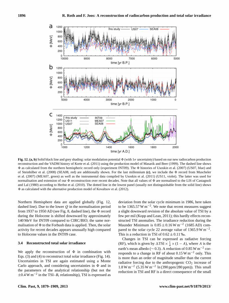
1896 R. Roth and F. Joos: A reconstruction of radiocarbon production and total solar irradiance
a
b
cINT09
Φ[M
eV
]
time [yr B.P.]
US07 SEA08this study
0
200
400
600
800
1000
1200
5000600070008000900010000
Φ[M
eV
]
time [yr B.P.]
0
200
400
600
800
1000
1200
010002000300040005000
Φ[M
eV
]
time [yr A.D.]
US11US07
MEA07SEA08
this study
0
200
400
600
800
1000
1200
1400
1000 1200 1400 1600 1800 2000
Fig. 12. (a, b)Solid black line and grey shading: solar modulation potential8 (with 1σ uncertainty) based on our new radiocarbon productionreconstruction and the VADM history ofKorte et al.(2011) using the production model ofMasarik and Beer(1999). The dashed line shows8 as calculated from the northern hemispheric record only (experiment INT09). The8 histories ofUsoskin et al.(2007) (US07, blue) andof Steinhilber et al.(2008) (SEA08, red) are additionally shown. For the last millennium(c), we include the8 record fromMuscheleret al. (2007) (MEA07, green) as well as the instrumental data compiled byUsoskin et al.(2011) (US11, violet). The latter was used fornormalisation and extension of our8 reconstruction over recent decades. Note that all values of8 are normalised to the LIS ofCastagnoliand Lal(1980) according toHerbst et al.(2010). The dotted line in the lowest panel (usually not distinguishable from the solid line) shows8 as calculated with the alternative production model ofKovaltsov et al.(2012).
Northern Hemisphere data are applied globally (Fig.12,dashed line). Due to the lowerQ in the normalisation periodfrom 1937 to 1950 AD (see Fig.8, dashed line), the8 recordduring the Holocene is shifted downward by approximately140 MeV for INT09 compared to CIRC/BIO; the same nor-malisation of8 to the Forbush data is applied. Then, the solaractivity for recent decades appears unusually high comparedto Holocene values in the INT09 case.
3.4 Reconstructed total solar irradiance
We apply the reconstruction of8 in combination withEqs. (3) and (4) to reconstruct total solar irradiance (Fig.14).Uncertainties in TSI are again estimated using a MonteCarlo approach, and considering uncertainties in8 and inthe parameters of the analytical relationship (but not the±0.4 W m−2 in the TSI–Br relationship), TSI is expressed as
deviation from the solar cycle minimum in 1986, here takento be 1365.57 W m−2. We note that recent measures suggesta slight downward revision of the absolute value of TSI by afew per mil (Kopp and Lean, 2011); this hardly effects recon-structed TSI anomalies. The irradiance reduction during theMaunder Minimum is 0.85± 0.16 W m−2 (1685 AD) com-pared to the solar cycle 22 average value of 1365.9 W m−2.This is a reduction in TSI of 0.62± 0.11 ‰.
Changes in TSI can be expressed as radiative forcing(RF), which is given by1TSI× 1
4 × (1− A), whereA is theearth’s mean albedo (∼ 0.3). A reduction of 0.85 W m−2 cor-responds to a change in RF of about 0.15 W m−2 only. Thisis more than an order of magnitude smaller than the currentradiative forcing due to the anthropogenic CO2 increase of1.8 W m−2 (5.35 W m−2 ln (390 ppm/280 ppm)). This smallreduction in TSI and RF is a direct consequence of the small
Clim. Past, 9, 1879–1909, 2013 www.clim-past.net/9/1879/2013/

R. Roth and F. Joos: A reconstruction of radiocarbon production and total solar irradiance 1897
6.0 6.5 7.0 7.5 8.0 8.5 9.0 9.5 10.0
geomagnetic field intensity [1022Am2 ]
200
300
400
500
600
700
800
900
sola
r m
odula
tion f
un
ctio
n [
MeV
]
1.41.5
1.6
1.7
1.8
1.92.02.12.2
2.3
count
count200
300
400
500
600
700
800
900
Fig. 13.The absolute radiocarbon production rate plotted as a func-tion of the solar modulation parameter8 and VADM. Yearly valuesof the smoothedQ record are used (with a cutoff period of 20 yras in Fig.10). The path taken by the model in this (8, VADM)-space is indicated by the thin grey line. The circle shows the value of8 for the normalisation period 1937–1950 as reported byUsoskinet al.(2011). The diamond shows the average production rate overthe entire Holocene. On the sides of the figure, two histograms aredisplayed showing the relative occurrence of certain VADM (toppanel) and8 (right panel) values,∼ 565 MeV being the medianmodulation potential during the Holocene.
slope in the relationship between TSI and the interplanetarymagnetic field as suggested byFrohlich(2009). Applying therelationships between TSI and8 suggested byShapiro et al.(2011) yields changes almost an order of magnitude larger inTSI and RF (right scale in Fig.14).
We compare our newly produced TSI record withtwo other recently published reconstructions based on ra-dionuclide production,Vieira et al. (2011) (VEA11) andSteinhilber et al.(2012) (SEA12). For the last millennium,the data fromDelaygue and Bard(2011) (DB11) is shownfor completeness. During three grand minima in the last mil-lennium, i.e. the Wolf, Sporer and Maunder minima, SEA12shows plateau-like values, apparently caused by a truncationof the 8 record to positive values. Also VEA11 suggestslower values during these minima compared to our recon-structions, but in general the differences in the TSI recon-structions are small, in particular when compared to the largeTSI variations suggested byShapiro et al.(2011).
Well-known solar periodicities in TSI contain the Hallstatt(2300 yr), Eddy (1000 yr), Suess (210 yr) and Gleissberg cy-cle (70–100 yr) as also discussed byWanner et al.(2008) andLundstedt et al.(2006). These periodicities are also presentin our reconstruction (Fig.15), as well as the long-term mod-ulation of approximately 6000 yr (Xapsos and Burke, 2009)(not shown). A wavelet (Morlet) power spectrum indicatesthat the power associated with the different cycles fluctuatedsomewhat during the Holocene.
We test the predictability of TSI given by its periodic na-ture to extrapolate insolation changes up to 2300 AD. Theextrapolation is calculated by fitting an autoregressive model(AR(p)) of orderp, applying Burg’s method (Kay, 1988) forparameter optimisation (Fig.15c). The order of the modelis the number of past time steps (i.e. years) used to fit themodel to the time series. We note that the spectrum of TSIis not strictly stationary (Fig.15b), limiting the confidencein forecasting future changes in TSI. We forecast TSI in thehistorical period (dashed lines in Fig.15c) to test to whichdegree TSI changes can be considered as an AR(p) process.Obviously, not all changes are matched in the historic pe-riod, although the present high values of TSI seems to bepredictable based on past TSI changes. Common to all ex-trapolations is the decreasing TSI in the next 10–20 yr to amagnitude comparable to 1900 AD. Towards 2200 AD, allthree extrapolations show again increasing TSI.
3.5 Changes in global mean surface air temperaturefrom total solar irradiance variability
We translate our new TSI record as well as two earlier re-constructions (VEA11, SEA12) into past changes in SAT us-ing the Bern3D-LPJ model. We follow the same protocolas in Sect.2.2. Two transient simulations were performedfor each TSI reconstruction: in one simulation TSI is keptconstant at its mean value, in the other simulation the ac-tual TSI reconstruction is applied.1SAT was then computedas the difference between the two simulations, normalised to1SAT = 0◦C in 2005 AD. As shown in Fig.16, the recon-structions yield rather small temperature changes attributedto solar forcing with|1SAT| less than 0.15◦C at any timeduring the Holocene. Compared to VEA12 and SEA12, ourTSI reconstruction results in less negative and more positivevalues in1SAT before 1900 AD as expected from the TSIrecord. No considerable TSI-induced long-term temperaturetrend is simulated. Applying our TSI reconstruction based ontheShapiro et al.(2011) scaling (green line and right scale inFig.16) translates into SAT changes≈ 6 times larger than theother reconstructions.
We note that our energy balance model does not take intoaccount spectral changes and changes in ultraviolet (UV)radiation, and thus related heating or cooling of the strato-sphere by the absorption of UV by ozone and other agents(Gray et al., 2010).
4 Summary and conclusions
In the present study the Holocene evolution of cosmogenicradiocarbon (14C) production is reconstructed using a stateof the art Earth system model of intermediate complexity andthe IntCal09/SHCal04 radiocarbon records. Then this pro-duction record is used in combination with reconstructionsof the geomagnetic field to reconstruct the solar modulation
www.clim-past.net/9/1879/2013/ Clim. Past, 9, 1879–1909, 2013

1898 R. Roth and F. Joos: A reconstruction of radiocarbon production and total solar irradiance
potential8. In further steps, total solar irradiance is recon-structed using recently proposed relationships between8
and TSI, and variations in TSI were translated into tempera-ture anomalies. The uncertainty arising from uncertainties ininput data, model parametrisation for the glacial termination,and model parameter values are propagated through the en-tire chain from production to solar modulation to TSI usingMonte Carlo and sensitivity simulations as well as Gaussianerror propagation.
The Bern3D-LPJ model is used to estimate radiocarbonproduction from the IntCal09/SHCal04 radiocarbon records.The model features a 3-D dynamic ocean component withan ocean sediment model and an interactive marine biolog-ical cycle, a 2-D atmosphere and a dynamic global vegeta-tion model component. The model is able to reproduce theobservation-based distributions of carbon and radiocarbonwithin the ocean as well as approximate the evolution of at-mospheric CO2 during the past 21 kyr. The explicit represen-tation of dissolved inorganic carbon and dissolved inorganicradiocarbon and the biological cycle in a 3-D dynamic settingis a step forward compared to the often applied perturbationapproach with the box diffusion model ofOeschger et al.(1975) or the outcrop model ofSiegenthaler(1983) (Vieiraet al., 2011; Usoskin and Kromer, 2005; Solanki et al., 2004;Muscheler et al., 2005b). These models underestimate by de-sign the inventory of dissolved inorganic carbon in the oceandue to the neglect of the marine biological cycle. Thus, themarine radiocarbon inventory and implied cosmogenic pro-duction is also underestimated. The Bern3D-LPJ carbon–climate model is forced with reconstructed changes in orbitalparameters, ice sheet extent influencing surface albedo, andnatural and anthropogenic variations in greenhouse gas con-centrations as well as sulfate aerosol forcings and climatevariations, thereby taking into account the influence of cli-matic variations on the cycling of carbon and radiocarbon.
Our production rate estimates can be compared to in-dependent estimates obtained with models that computeproduction of cosmogenic nuclides in the atmosphere bysimulating the interaction of incoming high energy parti-cles with atmospheric molecules (Masarik and Beer, 1999,2009). Masarik and Beer(2009) suggests a production of2.05± 0.2 atoms cm−2 s−1 for a solar modulation poten-tial of 550 MeV. The radiocarbon budget analysis yields alower production of 1.71 atoms cm−2 s−1 and for the same8. The Holocene mean14C production depends on varia-tions in 8 and the geomagnetic field and is estimated to1.77 atoms cm−2 s−1.
An open question was by how much uncertainties in thecarbon cycle processes leading to the deglacial CO2 rise af-fect estimates of the radiocarbon production. To this end, twoalternative, bounding scenarios for the deglacial CO2 risewere applied in addition to a control simulations with con-stant climate and ocean circulation. We show that uncertain-ties in the processes responsible for the reconstructed CO2and 114C variations over the glacial termination translate
into an uncertainty of the order of 5 % in the absolute mag-nitude of the production in the early Holocene, but only tosmall uncertainties in decadal to centennial production vari-ations. This uncertainty in millennial average production dueto the memory of the system to earlier changes vanishes overthe Holocene and becomes very small (< 1 %) in recent mil-lennia. Although a detailed process understanding of the ter-mination, e.g. the cause of the “mystery interval” (Broeckerand Barker, 2007), is not required to reconstruct radiocar-bon production in the Holocene, the decreasing trend in at-mospheric radiocarbon over the glacial termination must betaken into account.
Small differences between simulations that includeHolocene climate change and the control run with no cli-mate change are found. A caveat is that our 2-D atmosphericenergy and moisture balance model does not represent im-portant features of climate variability such as interannual anddecadal atmospheric modes. However, the available evidenceand the generally good agreement between14C-based andindependent solar proxy reconstructions suggest that atmo-spheric radiocarbon and inferred production are relatively in-sensitive to typical Holocene climate variations.
A prominent excursion in the early Holocene NorthernHemisphere climate is the 8.2 kyr BP event with a decreasein Greenland air temperature by about 3 K within a fewdecades (Kobashi et al., 2007). A reduction in North AtlanticDeep Water formation related to a spike in meltwater inputhas been proposed to have occurred with this event (Ellisonet al., 2006; Hoffman et al., 2012). This 8.2 kyr event isnot represented in our model setup, and a possible atmo-spheric radiocarbon signal from changing ocean circulation(e.g.Matsumoto and Yokoyama, 2013) would be erroneouslyattributed to a change in production.Vonmoos et al.(2006)compared solar modulation estimated from10Be versus14C.Deviations between the two reconstructions are not largerduring the 8.2 kyr event than during other early Holoceneperiods. Similarly, the different reconstructions shown inFig. 12 do not point to an exceptionally large imprint of the8.2 kyr event on inferred solar modulation and thus on radio-carbon production.
Solar modulation potential8 is computed using the re-lationship between radiocarbon production, the geomagneticdipole (Korte et al., 2011), and8 from the models ofMasarikand Beer(1999) andKovaltsov et al.(2012). A key step is thenormalisation of the14C-derived8 record to the Forbush in-strumental observations over the period 1937 to 1950 AD.Atmospheric114C is heavily contaminated after 1950 byatomic bomb tests, preventing a reliable extraction of the nat-ural production signal. In the mid-20th century, atmospheric114C and its interhemispheric gradient is influenced by theearly signals of fossil fuel combustion and land use. Our spa-tially resolved model allows us to treat interhemispheric con-centration differences and land use explicitly. We show thatreconstructions in8 that rely on the Northern Hemisphere114C record only are biased towards low values during the
Clim. Past, 9, 1879–1909, 2013 www.clim-past.net/9/1879/2013/

R. Roth and F. Joos: A reconstruction of radiocarbon production and total solar irradiance 1899
a
b
c
ΔT
SI [W
/m2]
ΔT
SI s
hapiro
[W/m
2]
time [yr B.P.]
VEA11 SEA12this study
-1.0
-0.5
0.0
0.5
1.0
5000600070008000900010000
-6
-4
-2
0
2
4
6
ΔT
SI [W
/m2]
ΔT
SI s
hapiro
[W/m
2]
time [yr B.P.]
-1.0
-0.5
0.0
0.5
1.0
010002000300040005000
-6
-4
-2
0
2
4
6
ΔT
SI [W
/m2]
ΔT
SI s
hapiro
[W/m
2]
time [yr A.D.]
DB11VEA11
SEA12PMOD
this study
-1.0
-0.5
0.0
0.5
1.0
1000 1200 1400 1600 1800 2000
-6
-4
-2
0
2
4
Fig. 14. (a, b)Total solar irradiance deviation from solar cycle minimum value in 1986 (assumed to 1365.57 W m−2) calculated in this study(black with grey 1σ error, lefty axis), and the reconstructions byVieira et al.(2011) (VEA11, red) andSteinhilber et al.(2012) (SEA12,blue). The dotted lines indicate the uncertainty introduced by random errors from the114C history alone excluding any systematic errors.(c) Magnification of the last 1000 yr; in addition to VEA11 and SEA12 the data ofDelaygue and Bard(2011) (DB11, green) is shown as wellas the composite record from the Physikalisch-Meteorologisches Observatorium Davos (PMOD). The DB11 record has been aligned to theother records by adding an offset of 0.5 W m−2. The righty axis shows the corresponding TSI variations when applying the8–TSI scalingof Shapiro et al.(2011) to our8 history.
Holocene. To our knowledge, the8 record byUsoskin et al.(2007) is based onQ from Usoskin and Kromer(2005) andthus on the Northern Hemisphere radiocarbon record only.Their values are systematically lower than ours and their bestestimates are in general outside our 1σ confidence band dur-ing the last 7 kyr. The8 record bySteinhilber et al.(2008)shows in general values below our confidence range duringthe period 7 to 3 kyr BP, while the two reconstructions agreeon average during the more recent millennia. Agreement withrespect to decadal to centennial variability is generally highamong the different reconstructions. However, notable ex-ceptions exist. For example, the reconstruction bySteinhilberet al.(2008) suggests a strong negative fluctuation between 8and 7.8 kyr BP, not seen in the14C-derived records.
We reevaluated the claim bySolanki et al.(2004) thatthe recent sun is exceptionally active. As earlier studies(Muscheler et al., 2007; Steinhilber et al., 2008), we con-clude that recent solar activity is high but not unusual in the
context of the Holocene.8 was estimated to be on averageat 650 MeV during the last 25 yr bySteinhilber et al.(2008)for a reference Local Interstellar Spectrum (LIS) ofCastag-noli and Lal(1980). We find an average8 for the Holocene(10 to 0 kyr BP) of 555 MeV. Solar activity in our decadallysmoothed record is during 28 % of the time higher than themodern average of 650 MeV and during 39 % of the timehigher than 600 MeV, used to define periods of high activityby Steinhilber et al.(2008) (Fig. 13). This may be comparedto corresponding values of 2 and 15 % bySteinhilber et al.(2008). In contrast to earlier reconstructions, our record sug-gests that periods of high solar activity (> 600 MeV) werequite common not only in recent millennia, but throughoutthe Holocene.
Our reconstruction in8 can be used to derive a rangeof solar irradiance reconstructions using published methods.Shapiro et al.(2011) suggest that variations in spectral andthus total solar irradiance are proportional to variation in8.
www.clim-past.net/9/1879/2013/ Clim. Past, 9, 1879–1909, 2013

1900 R. Roth and F. Joos: A reconstruction of radiocarbon production and total solar irradiance
period [yrs]p
eri
od
[yrs
]p
ow
er
[a.u
.]aSuess~210 yr
Eddy ~1000yrGleissberg~87 yr
b
c
0
5
10
15
20
100 1000
ΔT
SI [w
/m2]
-0.6-0.4-0.20.00.20.40.60.8
10000 9000 8000 7000 6000 5000 4000 3000 2000 1000
time [year B.P.]
64
128
256
512
1024
2048
1/256
1/64
1/16
1/4
1
4
16
Pow
er
[a.u
.]
0
time [yr A.D.]
ΔT
SI [w
/m2]
-0.6
-0.4
-0.2
0.0
0.2
0.4
0.6
1300 1500 1700 1900 2100 2300
AR(5000)
AR(10000)
AR(2000)futurepast
Fig. 15. (a)Power spectrum of our TSI record up to periodicities of 2000 yr. The most dominant periodicities correspond to the Gleissberg,Suess and Eddy cycles.(b) Wavelet power spectrum calculated with a Morlet wavelet with log2 periodicity axis and colour shading.(c) Fore-casting of the solar irradiance using an autoregressive model of orderp (AR(p)) fitted using Burg’s method. Before fitting the time series,a high-pass filter (1000 yr) has been applied in order to remove low-frequency trends. The dashed lines show forecasts with the AR(5000)model starting at year 1300, 1500, 1700 and 1900 AD (magenta dots). Coloured lines show forecasts starting in 2005 AD for different ordersof the AR model.
Their analysis suggests a high scaling of8 with TSI and aMaunder Minimum reduction in TSI compared to the presentsolar minimum by about 0.4 %. This is significantly largerthan the reduction suggested in other recent reconstructions(Steinhilber et al., 2012; Vieira et al., 2011), but within therange of TSI variations explored in earlier climate modelstudies (Ammann et al., 2007; Jansen et al., 2007). Here, wefurther converted8 into TSI using the nonlinear equationsused bySteinhilber et al.(2008). This yields small varia-tions in TSI and a Maunder Minimum reduction in TSI com-pared to recent solar minima of only 0.62 ‰. The resultingoverall range in TSI is about 1.2 W m−2. Future extensionof TSI using autoregressive modelling suggests a declining
solar activity in the next decades towards average Holoceneconditions.
We applied different TSI reconstructions to estimate vari-ations in global mean surface air temperature (SAT) due toTSI changes only. We stress that these SAT anomalies aredue to TSI variations only and do not include SAT varia-tions due to other drivers such as orbital forcing, natural andanthropogenic greenhouse gas concentration variations, orchanges in the extent and the albedo of ice sheets. The re-sults suggest that there were several periods in the Holocenewere TSI-related SAT anomalies were larger than for year2000 AD. In particular, several warm anomalies occurred inthe period from 5500 to 3600 BP. Temperature anomalies
Clim. Past, 9, 1879–1909, 2013 www.clim-past.net/9/1879/2013/

R. Roth and F. Joos: A reconstruction of radiocarbon production and total solar irradiance 1901
a
b
c
SEA12 VEA11this study
this study
ΔS
AT
[K
]
ΔS
AT
shapiro
[K]
time [yr B.P.]
-0.10
-0.05
0.00
0.05
5000600070008000900010000
-0.4
-0.2
0.0
0.2
0.4
ΔS
AT
[K
]
time [yr B.P.]
-0.10
-0.05
0.00
0.05
010002000300040005000
-0.4
-0.2
0.0
0.2
0.4
ΔS
AT
[K
]
time [yr A.D.]
-0.15
-0.10
-0.05
0.00
0.05
1000 1200 1400 1600 1800 2000
-0.4
-0.2
0.0
this study
SEA12 VEA11this study
ΔS
AT
shapiro
[K]
ΔS
AT
shapiro
[K]
Fig. 16. (a, b)Simulated changes in SAT as a response to different TSI forcings: this study (black), VEA11 (red) and SEA12 (blue), lefty
axis. The green line (righty axis) shows the simulated SAT changes by a solar variation based on our8 history but converted to TSI usingthe method ofShapiro et al.(2011). The anomalies were calculated as the difference between two transient simulations, one with all forcingsand the other with the same forcings but solar forcing taken to be constant. The last 1000 yr are shown again in(c). All lines show smoothingsplines with a cutoff period of 30 yr.
are comparable to twentieth century anomalies in the periodfrom 200 BC to 600 AD. In contrast, the TSI reconstructionof Steinhilber et al.(2012) implies that SAT anomalies dueto TSI changes were below current values almost during theentire Holocene. In conclusion, our reconstruction of the ra-diocarbon production rate and the solar modulation potential,as well as the implied changes in solar irradiance, provide analternative for climate modellers.
Appendix A
Estimation of uncertainties
A1 Assessment of uncertainties in the14C productionrecord
There are several potential sources of error entering the cal-culation of the production rate, summarised in Fig. A1. Asalready discussed in detail in the main text, the uncertain
deglacial carbon cycle changes translate into an uncertaintyin Q, especially in the early Holocene. To account for this,we use the arithmetic mean of BIO and CIRC as our bestguessQ reconstruction and the difference between them asour uncertainty range, which is around 4.5 % in the earlyHolocene and drops below 1 % at 5000 kyr BP.
In addition, also the uncertainty of the IntCal09/SHCal04record translates into an error of the production record.100 radiocarbon histories were randomly generated withGaussian-distributed114C values at each point in time of therecord, varied within 1σ uncertainty as (shown in Fig.2b) ontheir original time grid (5 yr spacing). For each realisation ofthe114C history, the transient simulation with Bern3D-LPJwas repeated and the resultingQ smoothed. The 1σ rangefrom the 100 smoothed records (Fig. A1b) is of the order of4–5 %, decreasing towards preindustrial times to 1.5 %.
During 1930–1950, this error increases again rapidly(hardly visible in Fig. A1b) to 10 % because the atmosphericcarbon inventory increases at a high rate. Therefore, rather
www.clim-past.net/9/1879/2013/ Clim. Past, 9, 1879–1909, 2013

1902 R. Roth and F. Joos: A reconstruction of radiocarbon production and total solar irradiance
a
b
c
d
e
f
production rate
350.0400.0450.0500.0550.0600.0650.0700.0
error from Δ14
C record
15.0
25.0
error from deglacial history
0.0
5.0
10.0
15.0
20.0
error from gas exchange/GPP
1.0
4.0
7.010.0
13.0
error from CO2-budget
0.0
5.0
10.0
15.0
time [year B.P.]
total error
10.0
20.0
30.0
0200040006000800010000
Fig. A1. Assessment of uncertainties in our production rate record in mol yr−1. (a) Radiocarbon production rate (arithmetic mean of CIRCand BIO);(b) the uncertainty stemming from the pre-Holocene carbon cycle evolution calculated as the absolute difference between resultsfrom simulations BIO and CIRC;(c) the smoothed 1σ error from the114C record (as shown in Fig.2b) is calculated by a Monte Carloapproach including 100 individual simulations; and(d) the uncertainty in air–sea and air–land fluxes deduced by sensitivity experiments.The total error in production(e)varies between 30 and 5 mol yr−1, corresponding to a relative error of∼ 6 to 1.5 %. The bulk uncertainty inthe average level ofQ resulting form an uncertain ocean (and land) inventory is not included in this calculation. We estimate this uncertaintyto be∼ 15 %.
small errors in114C of ∼ 1 ‰ translate into rather big un-certainties in the change of the atmospheric radiocarbon in-ventory, and thus into the production rate.
The air–sea flux of radiocarbon is the dominant flux outof the atmosphere with approximately 430 mol yr−1. We as-sess its variations by nominally changing the air–sea gas-exchange rate within±15 % (Muller et al., 2008). Two ad-ditional runs were performed in which the seasonally andspatially varying gas exchange rates of the standard setupwere increased/decreased everywhere by 15 %. In analogy,uncertainties in the flux into the land biosphere were assessedby varying the gross primary productivity of the model by±15 %. In these two experiments, differences in the total14C inventory were subtracted to get the uncertainties in thefluxes alone; the effect of the inventory is discussed sep-arately. These errors in14Fas +
14Fab vary together withchanges in the atmospheric114C signature. The error fromthe uncertainty in the combined air-to-sea and air-to-land(14Fas +
14Fab) fluxes is smaller than 2.5 % of the produc-tion at any time (Fig. A1d). It is important to note that the
uncertainty in gas exchange and GPP do not alter the abso-lute value ofQ, but change the amplitude in the variationsof Q.
Uncertainties are also related to the14C signature associ-ated with the carbon flux applied to close the atmosphericCO2 budget (14Fbudget in Eq. 1). For example, the missingcarbon sink process could be due to a slow down of theoceanic thermohaline circulation (THC) or a growth of landvegetation: two processes with different isotopic signatures.We assume that this signature varies between±200 ‰ rel-ative to the contemporary atmosphere. The associated errorin the production is in general small with peaks of 1–2 %(Fig. A1e). However, towards 1950 AD, where the anthro-pogenic influence leads to increasing CO2 levels, the uncer-tainty reaches up to 4 % as the model simulates a too-weakoceanic/land sink and/or too-high emissions.
We estimate the total standard deviation by quadratic er-
ror addition,σQ =√∑
σ 2Q,i , to be ∼ 6 % during the early
Holocene, decreasing to 1.5–2.5 % towards preindustrialtimes (Fig. A1f). The total uncertainty in the early Holocene
Clim. Past, 9, 1879–1909, 2013 www.clim-past.net/9/1879/2013/

R. Roth and F. Joos: A reconstruction of radiocarbon production and total solar irradiance 1903
a
b
c
d
e
Φ
0.0
200.0
400.0
600.0
800.0
1000.0
1200.0
error from Q
30.0
60.0
90.0
120.0
error from VADM
50.0
100.0
150.0
200.0
error from production model
20.0
40.0
60.0
80.0
100.0
time [year B.P.]
total error
50.0100.0150.0200.0250.0300.0
0200040006000800010000
Fig. A2. Assessment of uncertainties in the solar modulation potential8 in MeV. (a) Best estimate of8 (mean of the Monte Carlo simu-lations),(b) uncertainty in8 from uncertainties in the radiocarbon productionQ, (c) from the uncertainty in the VADM reconstruction byKorte et al.(2011), (d) the uncertainty in the model to convert production into8, and(e) total 1σ uncertainty in the MC calculation.
is dominated by the uncertainty in the114C input dataand the deglacial history. These two sources of error de-crease towards preindustrial times. In the first half of thelast century, uncertainties increase again mainly associatedwith the anthropogenic CO2 increase. This increasing uncer-tainty towards 1950 AD (∼ 9 %) is important when normalis-ing reconstructed solar modulation to the recent instrumentalrecords.
As noted in the main text, the 1σ error is estimated to be15 % for the ocean14C inventory (R. Key, personal commu-nication, May 2013) and for the total14C inventory. This po-tential systematic bias is not included in the uncertainty bandof Q as it would not change the temporal evolution.
A2 Propagation of uncertainties fromQ to 8 and1TSI
Next, the uncertainty calculation of8 and of1TSI is dis-cussed (grey bands in Figs.12and14). Three general sourcesof uncertainty in8 are considered: the uncertainty inQ, theuncertainty in VADM and finally the error of the produc-tion rate simulations (i.e. the slope of8/Q) assumed to be10 %. Using Monte Carlo calculations, we varied the differ-ent sources of uncertainty individually in every year to as-sess the propagation of errors. In Fig. A2b–d the individual
1σ errors of this calculation are shown. The total error in8
varies then between 300 MeV (early Holocene) and 70 MeV(preindustrial). All three components of error contribute toapproximately equal parts to the total uncertainty.
The possible bias introduced by the normalisation is notincluded in this figure. This would add another∼ 130 MeVuncertainty to the average level of8 (but not on its tempo-ral evolution). Note that any constant systematic offset inQ
would not translate into an offset in the solar modulation po-tential asQ is normalised before converting to8.
Similarly, the uncertainty in the change in TSI as re-constructed with the use of Eqs. (3) and (4) is calculated(Fig. A3b and c). The 1σ error of 8 is taken into accountas well as the uncertainties in Eq. (4) and of the exponentαin Eq. (3) (±0.3) (Steinhilber et al., 2009). The error in thereference value of TSI (1264.64 W m−2 in Eq. 4) does notaffect relative changes in TSI, but its absolute level. The total1σ uncertainty in1TSI ranges between 0.2 and 0.8 W m−2
(Fig. A3d), to equal part stemming from the error in8 andthe conversion model.
More than half of the uncertainty in TSI is of system-atic nature and related to the8–TSI relationship (Fig. A3c).More specifically, the slope of the linear relationship between
www.clim-past.net/9/1879/2013/ Clim. Past, 9, 1879–1909, 2013
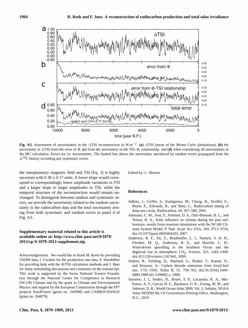
1904 R. Roth and F. Joos: A reconstruction of radiocarbon production and total solar irradiance
a
b
c
ΔTSI
-0.60-0.40-0.200.000.200.400.600.801.00
error from Φ
0.10
0.20
0.30
0.40
0.50
error from Φ-TSI relationship
0.10
0.20
0.30
0.40
0.50
time [year B.P.]
total error
0.00
0.20
0.40
0.60
0.80
0200040006000800010000
random error from Δ14C forcing
d
Fig. A3. Assessment of uncertainties in the1TSI reconstruction in W m−2. (a) 1TSI (mean of the Monte Carlo simulations),(b) theuncertainty in1TSI from the error of8, (c) from the uncertainty in the TSI–Br relationship, and(d) when considering all uncertainties inthe MC calculation. Errors are 1σ uncertainties. The dashed line shows the uncertainty introduced by random errors propagated from the114C history excluding any systematic errors.
the interplanetary magnetic field and TSI (Eq.3) is highlyuncertain with 0.38± 0.17 units. A lower slope would corre-spond to correspondingly lower amplitude variations in TSIand a larger slope to larger amplitudes in TSI, while thetemporal structure of the reconstruction would remain un-changed. To distinguish between random and systematic er-rors, we provide the uncertainty related to the random uncer-tainty in the radiocarbon data and the total uncertainty aris-ing from both systematic and random errors in panel d ofFig. A3.
Supplementary material related to this article isavailable online at:http://www.clim-past.net/9/1879/2013/cp-9-1879-2013-supplement.zip.
Acknowledgements.We would like to thank M. Korte for providingVADM data, I. Usoskin for the production rate data, F. Steinhilberfor providing help with the8/TSI calculation methods and J. Beerfor many stimulating discussions and comments on the manuscript.This work is supported by the Swiss National Science Founda-tion through the National Centre for Competence in Research(NCCR) Climate and by the grant to Climate and EnvironmentalPhysics and support by the European Commission through the FP7projects Past4Future (grant no. 243908) and CARBOCHANGE(grant no. 264879).
Edited by: L. Skinner
References
Adkins, J., Griffin, S., Kashgarian, M., Cheng, H., Druffel, E.,Boyle, E., Edwards, R., and Shen, C.: Radiocarbon dating ofdeep-sea corals, Radiocarbon, 44, 567–580, 2002.
Ammann, C. M., Joos, F., Schimel, D. S., Otto-Bliesner, B. L., andTomas, R. A.: Solar influence on climate during the past mil-lennium: results from transient simulations with the NCAR Cli-mate System Model, P. Natl. Acad. Sci. USA, 104, 3713–3718,doi:10.1073/pnas.0605064103, 2007.
Anderson, R. F., Ali, S., Bradtmiller, L. I., Nielsen, S. H. H.,Fleisher, M. Q., Anderson, B. E., and Burckle, L. H.:Wind-driven upwelling in the Southern Ocean and thedeglacial rise in atmospheric CO2, Science, 323, 1443–1448,doi:10.1126/science.1167441, 2009.
Andres, R., Fielding, D., Marland, G., Boden, T., Kumar, N.,and Kearney, A.: Carbon dioxide emissions from fossil-fueluse, 1751–1950, Tellus B, 51, 759–765, doi:10.1034/j.1600-0889.1999.t01-3-00002.x, 1999.
Antonov, J. I., Seidov, D., Boyer, T. P., Locarnini, R. A., Mis-honov, A. V., Garcia, H. E., Baranova, O. K., Zweng, M. M., andJohnson, D. R.: World Ocean Atlas 2009, Vol. 2: Salinity, NOAAAtlas NESDIS 68, US Government Printing Office, Washington,D.C., 2010.
Clim. Past, 9, 1879–1909, 2013 www.clim-past.net/9/1879/2013/

R. Roth and F. Joos: A reconstruction of radiocarbon production and total solar irradiance 1905
Bard, E., Raisbeck, G., Yiou, F., and Jouzel, J.: Solar modulation ofcosmogenic nuclide production over the last millennium: com-parison between C-14 and Be-10 records, Earth Planet. Sc. Lett.,150, 453–462, doi:10.1016/S0012-821X(97)00082-4, 1997.
Bard, E., Raisbeck, G., Yiou, F., and Jouzel, J.: Solar irradiance dur-ing the last 1200 years based on cosmogenic nuclides, Tellus B,52, 985–992, doi:10.1034/j.1600-0889.2000.d01-7.x, 2000.
Bauer, J. E., Williams, P. M., and Druffel, E. R. M.:14C activityof dissolved organic carbon fractions in the north-central Pacificand Sargasso Sea, Nature, 357, 667–670, doi:10.1038/357667a0,1992.
Beer, J., Andree, M., Oeschger, H., Stauffer, B., Balzer, R., Bo-nani, G., Stoller, C., Suter, M., Wolfli, W., and Finkel, R. C.:Temporal 10Be variations in ice, Radiocarbon, 25, 269–278,1983.
Berger, A. L.: Long-term variations of daily insolation and quater-nary climatic changes, J. Atmos. Sci., 35, 2362–2367, 1978.
Bouttes, N., Paillard, D., Roche, D. M., Brovkin, V., and Bopp, L.:Last Glacial Maximum CO2 andδ13C successfully reconciled,Geophys. Res. Lett., 38, L02705, doi:10.1029/2010GL044499,2011.
Broecker, W. and Barker, S.: A 190 ‰ drop in atmosphere’s114Cduring the ”Mystery Interval” (17.5 to 14.5 kyr), Earth Planet.Sc. Lett. 256, 90–99, doi:10.1016/j.epsl.2007.01.015, 2007.
Brovkin, V., Ganopolski, A., Archer, D., and Rahmstorf, S.: Lower-ing of glacial atmospheric CO2 in response to changes in oceaniccirculation and marine biogeochemistry, Paleoceanography, 22,PA4202, doi:10.1029/2006PA001380, 2007.
Brovkin, V., Ganopolski, A., Archer, D., and Munhoven, G.: GlacialCO2 cycle as a succession of key physical and biogeochemicalprocesses, Clim. Past, 8, 251–264, doi:10.5194/cp-8-251-2012,2012.
Bryan, S. P., Marchitto, T. M., and Lehman, S. J.: The releaseof 14C-depleted carbon from the deep ocean during the lastdeglaciation: evidence from the Arabian Sea, Earth Planet. Sc.Lett., 298, 244–254, doi:10.1016/j.epsl.2010.08.025, 2010.
Burke, A. and Robinson, L. F.: The Southern Ocean’s role in carbonexchange during the last deglaciation, Science, 335, 557–561,doi:10.1126/science.1208163, 2012.
Castagnoli, G. and Lal, D.: Solar modulation effects in terrestrialproduction of carbon-14, Radiocarbon, 22, 133–158, 1980.
Clark, P. U., Shakun, J. D., Baker, P. A., Bartlein, P. J., Brewer, S.,Brook, E., Carlson, A. E., Cheng, H., Kaufman, D. S.,Liu, Z., Marchitto, T. M., Mix, A. C., Morrill, C., Otto-Bliesner, B. L., Pahnke, K., Russell, J. M., Whitlock, C., Ad-kins, J. F., Blois, J. L., Clark, J., Colman, S. M., Curry, W. B.,Flower, B. P., He, F., Johnson, T. C., Lynch-Stieglitz, J.,Markgraf, V., McManus, J., Mitrovica, J. X., Moreno, P. I.,and Williams, J. W.: Global climate evolution during the lastdeglaciation, P. Natl. Acad. Sci. USA, 109, E1134–E1142,doi:10.1073/pnas.1116619109, 2012.
Crowley, T. J.: Causes of climate change over the past 1000 years,Science, 289, 270–277, doi:10.1126/science.289.5477.270,2000.
Delaygue, G. and Bard, E.: An Antarctic view of beryllium-10 andsolar activity for the past millennium, Clim. Dynam., 36, 2201–2218, doi:10.1007/s00382-010-0795-1, 2011.
De Pol-Holz, R., Keigwin, L., Southon, J., Hebbeln, D., and Mo-htadi, M.: No signature of abyssal carbon in intermediate wa-ters off Chile during deglaciation, Nat. Geosci., 3, 192–195,doi:10.1038/ngeo745, 2010.
Edwards, N. R. and Marsh, R.: Uncertainties due to transport-parameter sensitivity in an efficient 3-D ocean-climate model,Clim. Dynam., 24, 415–433, doi:10.1007/s00382-004-0508-8,2005.
Ellison, C. R. W., Chapman, M. R., and Hall, I. R.: Surface and deepocean interactions during the cold climate event 8200 years ago,Science, 312, 1929–1932, doi:10.1126/science.1127213, 2006.
Elsig, J., Schmitt, J., Leuenberger, D., Schneider, R., Eyer, M.,Leuenberger, M., Joos, F., Fischer, H., and Stocker, T. F.:Stable isotope constraints on Holocene carbon cyclechanges from an Antarctic ice core, Nature, 461, 507–510,doi:10.1038/nature08393, 2009.
Enting, I. G.: On the use of smoothing splines to fil-ter CO2 data, J. Geophys. Res., 92, 10977–10984,doi:10.1029/JD092iD09p10977, 1987.
Farquhar, G. D., Caemmerer, S. V., and Berry, J. A.: A biochemical-model of photosynthetic CO2 assimilation in leaves of C-3species, Planta, 149, 78–90, 1980.
Feely, R., Sabine, C., Lee, K., Berelson, W., Kleypas, J.,Fabry, V., and Millero, F.: Impact of anthropogenic CO2 onthe CaCO3 system in the oceans, Science, 305, 362–366,doi:10.1126/science.1097329, 2004.
Francey, R., Allison, C., Etheridge, D., Trudinger, C., Enting, I.,Leuenberger, M., Langenfelds, R., Michel, E., and Steele, L.:A 1000-year high precision record ofδ13C in atmosphericCO2, Tellus B, 51, 170–193, doi:10.1034/j.1600-0889.1999.t01-1-00005.x, 1999.
Franois, R., Altabet, M. A., Yu, E.-F., Sigman, D. M., Bacon, M. P.,Frank, M., Bohrmann, G., Bareille, G., and Labeyrie, L. D.: Con-tribution of Southern Ocean surface-water stratification to lowatmospheric CO2 concentrations during the last glacial period,Nature, 389, 929–935, doi:10.1038/40073, 1997.
Frohlich, C.: Evidence of a long-term trend in total solar irra-diance, Astron. Astrophys., 501, L27–L30, doi:10.1051/0004-6361/200912318, 2009.
Galbraith, E. D., Jaccard, S. L., Pedersen, T. F., Sigman, D. M.,Haug, G. H., Cook, M., Southon, J. R., and Francois, R.: Car-bon dioxide release from the North Pacific abyss during the lastdeglaciation, Nature, 449, 890–893, doi:10.1038/nature06227,2007.
Gehlen, M., Bopp, L., Emprin, N., Aumont, O., Heinze, C., andRagueneau, O.: Reconciling surface ocean productivity, exportfluxes and sediment composition in a global biogeochemicalocean model, Biogeosciences, 3, 521–537, doi:10.5194/bg-3-521-2006, 2006.
Gerber, S., Joos, F., Brugger, P., Stocker, T. F., Mann, M. E.,Sitch, S., and Scholze, M.: Constraining temperature varia-tions over the last millennium by comparing simulated andobserved atmospheric CO2, Clim. Dynam., 20, 281–299,doi:10.1007/s00382-002-0270-8, 2003.
Gleeson, L. and Axford, W.: Solar modulation of galactic cosmicrays, Astrophys. J., 154, 1011–1026, doi:10.1086/149822, 1968.
www.clim-past.net/9/1879/2013/ Clim. Past, 9, 1879–1909, 2013
1906 R. Roth and F. Joos: A reconstruction of radiocarbon production and total solar irradiance
Gray, L. J., Beer, J., Geller, M., Haigh, J. D., Lockwood, M.,Matthes, K., Cubasch, U., Fleitmann, D., Harrison, G., Hood, L.,Luterbacher, J., Meehl, G. A., Shindell, D., van Geel, B., andWhite, W.: Solar influences on climate, Rev. Geophys., 48,RG4001, doi:10.1029/2009RG000282, 2010.
Griffies, S. M.: The Gent–Williams skew flux,J. Phys. Oceanogr., 28, 831–841, doi:10.1175/1520-0485(1998)028<0831:TGMSF>2.0.CO;2, 1998.
Hambaryan, V. V. and Neuhauser, R.: A galactic short gamma-rayburst as cause for the14C peak in AD 774/5, Mon. Not. R. As-tron. Soc., doi:10.1093/mnras/sts378, 430, 32–36, 2013.
Hansell, D. A., Carlson, C. A., Repeta, D. J., and Schlitzer, R.: Dis-solved organic matter in the ocean a controversy stimulates newinsights, Oceanography, 22, 202–211, 2009.
Heinze, C., Maier-Reimer, E., Winguth, A. M. E., and Archer, D.:A global oceanic sediment model for long-term climate studies,Global Biogeochem. Cy., 13, 221–250, 1999.
Herbst, K., Kopp, A., Heber, B., Steinhilber, F., Fichtner, H.,Scherer, K., and Matthia, D.: On the importance of the local inter-stellar spectrum for the solar modulation parameter, J. Geophys.Res., 115, D00I20, doi:10.1029/2009JD012557, 2010.
Hodell, D. A., Venz, K. A., Charles, C. D., and Ninnemann, U. S.:Pleistocene vertical carbon isotope and carbonate gradients in theSouth Atlantic sector of the Southern Ocean, Geochem. Geophy.Geosy., 4, 1–19, doi:10.1029/2002GC000367, 2003.
Hoffman, J. S., Carlson, A. E., Winsor, K., Klinkhammer, G. P.,LeGrande, A. N., Andrews, J. T., Strasser, J. C.: Linking the8.2 ka event and its freshwater forcing in the labrador sea, Geo-phys. Res. Lett., 39, L18703, doi:10.1029/2012GL053047, 2012.
Hughen, K., Baillie, M., Bard, E., Beck, J., Bertrand, C., Black-well, P., Buck, C., Burr, G., Cutler, K., Damon, P., Edwards, R.,Fairbanks, R., Friedrich, M., Guilderson, T., Kromer, B., McCor-mac, G., Manning, S., Ramsey, C., Reimer, P., Reimer, R., Rem-mele, S., Southon, J., Stuiver, M., Talamo, S., Taylor, F., van derPlicht, J., and Weyhenmeyer, C.: Marine04 marine radiocarbonage calibration, 0–26 cal kyr BP, Radiocarbon, 46, 1059–1086,2004.
Jackson, A., Jonkers, A. R. T., and Walker, M. R.: Four centuriesof geomagnetic secular variation from historical records, Phi-los. T. Roy. Soc. A, 358, 957–990, doi:10.1098/rsta.2000.0569,2000.
Jansen, E., Overpeck, J., Briffa, K. R., Duplessy, J.-C.,Joos, F., Masson-Delmotte, V., Olago, D., Otto-Bliesner, B.,Peltier, W. R., Rahmstorf, S., Ramesh, R., Raynaud, D., Rind, D.,Solomina, O., Villalba, R., and Zhang, D.: Palaeoclimate, in:Climate Change 2007: The Physical Science Basis. WorkingGroup I Contribution to the Fourth Assessment Report ofthe Intergovernmental Panel on Climate Change, edited by:Solomon, S., Qin, D., Manning, M., Chen, Z., Marquis, M., Av-eryt, K. B., Tignor, M., and Miller, H. L., Cambridge UniversityPress, 433–497, 2007.
Joos, F. and Spahni, R.: Rates of change in natu-ral and anthropogenic radiative forcing over the past20,000 years, P. Natl. Acad. Sci. USA, 105, 1425–1430,doi:10.1073/pnas.0707386105, 2008.
Joos, F., Prentice, I. C., Sitch, S., Meyer, R., Hooss, G., Plat-tner, G.-K., Gerber, S., and Hasselmann, K.: Global warmingfeedbacks on terrestrial carbon uptake under the Intergovernmen-tal Panel on Climate Change (IPCC) emission scenarios, Global
Biogeochem. Cy., 15, 891–907, 2001.Joos, F., Gerber, S., Prentice, I. C., Otto-Bliesner, B. L.,
and Valdes, P. J.: Transient simulations of Holocene atmo-spheric carbon dioxide and terrestrial carbon since the LastGlacial Maximum, Global Biogeochem. Cy., 18, GB2002,doi:10.1029/2003GB002156, 2004.
Jungclaus, J. H., Lorenz, S. J., Timmreck, C., Reick, C. H., Brovkin,V., Six, K., Segschneider, J., Giorgetta, M. A., Crowley, T. J.,Pongratz, J., Krivova, N. A., Vieira, L. E., Solanki, S. K., Klocke,D., Botzet, M., Esch, M., Gayler, V., Haak, H., Raddatz, T. J.,Roeckner, E., Schnur, R., Widmann, H., Claussen, M., Stevens,B., and Marotzke, J.: Climate and carbon-cycle variability overthe last millennium, Clim. Past, 6, 723–737, doi:10.5194/cp-6-723-2010, 2010.
Kalnay, E., Kanamitsu, M., Kistler, R., Collins, W., Deaven, D.,Gandin, L., Iredell, M., Saha, S., White, G., Woollen, J.,Zhu, Y., Chelliah, M., Ebisuzaki, W., Higgins, W., Janowiak, J.,Mo, K., Ropelewski, C., Wang, J., Leetmaa, A., Reynolds, R.,Jenne, R., and Joseph, D.: The NCEP/NCAR 40-year reanalysisproject, B. Am. Meteorol. Soc., 77, 437–471, doi:10.1175/1520-0477(1996)077<0437:TNYRP>2.0.CO;2, 1996.
Kay, S. M.: Modern Spectral Estimation: Theory and Application,Prentice-Hall, Englewood Cliffs, N.J., 1988.
Key, R. M., Kozyr, A., Sabine, C. L., Lee, K., Wanninkhof, R.,Bullister, J. L., Feely, R. A., Millero, F. J., Mordy, C., andPeng, T.-H.: A global ocean carbon climatology: results fromGlobal Data Analysis Project (GLODAP), Global Biogeochem.Cy., 18, GB4031,doi:10.1029/2004GB002247, 2004.
Klein Goldewijk, K.: Estimating global land use change over thepast 300 years: the HYDE database, Global Biogeochem. Cy.,15, 417–433, 2001.
Klein Goldewijk, K. and van Drecht, G.: HYDE3: current andhistorical population and land cover, in: Integrated Mod-elling of Global Environmental Change, An Overview of IM-AGE 2.4., edited by: Bouwman, A. F., Kram, T., and KleinGoldewijk, K., Netherlands Environmental Assessment Agency(MNP), Bilthoven, the Netherlands, 2006.
Knudsen, M. F., Riisager, P., Donadini, F., Snowball, I.,Muscheler, R., Korhonen, K., and Pesonen, L. J.: Varia-tions in the geomagnetic dipole moment during the Holoceneand the past 50 kyr, Earth Planet. Sc. Lett., 272, 319–329,doi:10.1016/j.epsl.2008.04.048, 2008.
Kobashi, T., Severinghaus, J. P., Brook, E. J., Barnola, J.-M., and Grachev, A. M.: Precise timing and characteriza-tion of abrupt climate change 8200 years ago from airtrapped in polar ice, Quaternary Sci. Rev., 26, 1212–1222,doi:10.1016/j.quascirev.2007.01.009, 2007.
Kohler, P., Fischer, H., Munhoven, G., and Zeebe, R.: Quan-titative interpretation of atmospheric carbon records over thelast glacial termination, Global Biogeochem. Cy., 19, GB4020,doi:10.1029/2004GB002345, 2005.
Kopp, G. and Lean, J. L.: A new, lower value of total solar irradi-ance: evidence and climate significance, Geophys. Res. Lett., 38,L01706, doi:10.1029/2010GL045777, 2011.
Korte, M., Constable, C., Donadini, F., and Holme, R.: Reconstruct-ing the Holocene geomagnetic field, Earth Planet. Sc. Lett., 312,497–505, doi:10.1016/j.epsl.2011.10.031, 2011.
Clim. Past, 9, 1879–1909, 2013 www.clim-past.net/9/1879/2013/
R. Roth and F. Joos: A reconstruction of radiocarbon production and total solar irradiance 1907
Kovaltsov, G. A., Mishev, A., and Usoskin, I. G.: A newmodel of cosmogenic production of radiocarbon14C inthe atmosphere, Earth Planet. Sc. Lett., 337–338, 114–120,doi:10.1016/j.epsl.2012.05.036, 2012.
Krakauer, N. Y., Randerson, J. T., Primeau, F. W., Gruber, N., andMenemenlis, D.: Carbon isotope evidence for the latitudinal dis-tribution and wind speed dependence of the air–sea gas transfervelocity, 7th International Carbon Dioxide Conference (CO2),Boulder, CO, 25–30 September 2005, Tellus B, 58, 390–417,doi:10.1111/j.1600-0889.2006.00223.x, 2006.
Kwon, E. Y., Primeau, F., and Sarmiento, J. L.: The impact of rem-ineralization depth on the air–sea carbon balance, Nat. Geosci.,2, 630–635, doi:10.1038/ngeo612, 2009.
Lambert, F., Delmonte, B., Petit, J. R., Bigler, M., Kaufmann, P. R.,Hutterli, M. A., Stocker, T. F., Ruth, U., Steffensen, J. P., andMaggi, V.: Dust-climate couplings over the past 800,000-yearsfrom the EPICA Dome C ice core, Nature, 452, 616–619,doi:10.1038/nature06763, 2008.
Lean, J.: Evolution of the Sun’s spectral irradiance since theMaunder Minimum, Geophys. Res. Lett., 27, 2425–2428,doi:10.1029/2000GL000043, 2000.
Lisiecki, L. E. and Raymo, M. E.: A Pliocene-Pleistocene stack of57 globally distributed benthicδ18O records, Paleoceanography,20, PA1003, doi:10.1029/2004PA001071, 2005.
Locarnini, R. A., Mishonov, A. V., Antonov, J. I., Boyer, T. P., Gar-cia, H. E., Baranova, O. K., Zweng, M. M., and Johnson, D. R.:World Ocean Atlas 2009, Vol. 1: Temperature, NOAA AtlasNESDIS 68, US Government Printing Office, Washington, D.C.,2010.
Lockwood, M.: Solar change and climate: an update in the light ofthe current exceptional solar minimum, P. Natl. Acad. Sci. USA,466, 303–329, doi:10.1098/rspa.2009.0519, 2010.
Lockwood, M.: Solar influence on global and regional climates,Surv. Geophys., 33, 503–534, doi:10.1007/s10712-012-9181-3,2012.
Lockwood, M. and Owens, M. J.: Centennial changes in theheliospheric magnetic field and open solar flux: the con-sensus view from geomagnetic data and cosmogenic iso-topes and its implications, J. Geophys. Res., 116, A04109,doi:10.1029/2010JA016220, 2011.
Lundstedt, H., Liszka, L., Lundin, R., and Muscheler, R.: Long-termsolar activity explored with wavelet methods, Ann. Geophys., 24,769–778, doi:10.5194/angeo-24-769-2006, 2006.
Luo, C., Mahowald, N. M., and del Corral, J.: Sensitivity studyof meteorological parameters on mineral aerosol mobiliza-tion, transport, and distribution, J. Geophys. Res., 108, 4447,doi:10.1029/2003JD003483, 2003.
MacFarling Meure, C., Etheridge, D., Trudinger, C., Steele, P.,Langenfelds, R., van Ommen, T., Smith, A., and Elkins, J.:Law Dome CO2, CH4 and N2O ice core records ex-tended to 2000 years BP, Geophys. Res. Lett., 33, L14810,doi:10.1029/2006GL026152, 2006.
Mahowald, N. M., Muhs, D. R., Levis, S., Rasch, P. J., Yosh-ioka, M., Zender, C. S., and Luo, C.: Change in atmospheric min-eral aerosols in response to climate: last glacial period, preindus-trial, modern, and doubled carbon dioxide climates, J. Geophys.Res., 111, D10202, doi:10.1029/2005JD006653, 2006.
Marchal, O.: Optimal estimation of atmospheric14C productionover the Holocene: paleoclimate implications, Clim. Dynam., 24,71–88, doi:10.1007/s00382-004-0476-z, 2005.
Marchitto, T. M., Lehman, S. J., Ortiz, J. D., Fluckiger, J., and vanGeen, A.: Marine radiocarbon evidence for the mechanism ofdeglacial atmospheric CO2 rise, Science, 316, 1456–1459, 2007.
Masarik, J. and Beer, J.: Simulation of particle fluxes and cosmo-genic nuclide production in the Earth’s atmosphere, J. Geophys.Res., 104, 12099–12111, doi:10.1029/1998JD200091, 1999.
Masarik, J. and Beer, J.: An updated simulation of particle fluxesand cosmogenic nuclide production in the Earth’s atmosphere,J. Geophys. Res., 114, D11103, doi:10.1029/2008JD010557,2009.
Matsumoto, K.: Biology-mediated temperature control on atmo-sphericpCO2 and ocean biogeochemistry, Geophys. Res. Lett.,34, L20605, doi:10.1029/2007GL031301, 2007.
Matsumoto, K. and Yokoyama, Y.: Atmospheric114C reduction insimulations of Atlantic overturning circulation shutdown GlobalBiogeochem. Cy., 27, 296–304, doi:10.1002/gbc.20035, 2013.
McCormac, F., Hogg, A., Blackwell, P., Buck, C., Higham, T.,and Reimer, P.: SHCal04 Southern Hemisphere calibration, 0–11.0 cal kyr BP, Radiocarbon, 46, 1087–1092, 2004.
Menviel, L. and Joos, F.: Toward explaining the Holocene car-bon dioxide and carbon isotope records: results from transientocean carbon cycle-climate simulations, Paleoceanography, 27,PA1207, doi:10.1029/2011PA002224, 2012.
Menviel, L., Joos, F., and Ritz, S.: Simulating atmosphericCO2, 13C and the marine carbon cycle during the LastGlacial-Interglacial cycle: possible role for a deepening ofthe mean remineralization depth and an increase in theoceanic nutrient inventory, Quaternary Sci. Rev., 56, 46–68,doi:10.1016/j.quascirev.2012.09.012, 2012.
Miyake, F., Nagaya, K., Masuda, K., and Nakamura, T.: A signatureof cosmic-ray increase in ad 774–775 from tree rings in Japan,Nature, 486, 240–242, doi:10.1038/nature11123, 2012.
Monnin, E., Steig, E. J., Siegenthaler, U., Kawamura, K., Schwan-der, J., Stauffer, B., Stocker, T. F., Morse, D. L., Barnola, J.-M., Bellier, B., Raynaud, D., and Fischer, H.: Evidence for sub-stantial accumulation rate variability in Antarctica during theHolocene, through synchronization of CO2 in the Taylor Dome,Dome C and DML ice cores, Earth Planet. Sc. Lett., 224, 45–54,doi:10.1016/j.epsl.2004.05.007, 2004.
Muller, S. A., Joos, F., Edwards, N. R., and Stocker, T. F.: Watermass distribution and ventilation time scales in a cost-efficient,three-dimensional ocean model, J. Climate, 19, 5479–5499,doi:10.1175/JCLI3911.1, 2006.
Muller, S. A., Joos, F., Edwards, N. R., and Stocker, T. F.: Modelednatural and excess radiocarbon: sensitivities to the gas exchangeformulation and ocean transport strength, Global Biogeochem.Cy., 22, GB3011, doi:10.1029/2007GB003065, 2008.
Muscheler, R., Beer, J., Kubik, P. W., and Synal, H.-A.: Geomag-netic field intensity during the last 60,000 years based on10Beand 36Cl from the Summit ice cores and14C, Quaternary Sci.Rev., 24, 1849–1860, 2005a.
Muscheler, R., Joos, F., Muller, S. A., and Snowball, I.: Climate:how unusual is today’s solar activity?, Nature, 436, E3–E4,doi:10.1038/nature04045, 2005b.
www.clim-past.net/9/1879/2013/ Clim. Past, 9, 1879–1909, 2013

1908 R. Roth and F. Joos: A reconstruction of radiocarbon production and total solar irradiance
Muscheler, R., Joos, F., Beer, J., Muller, S. A., Vonmoos, M.,and Snowball, I.: Solar activity during the last 1000 yr inferredfrom radionuclide records, Quaternary Sci. Rev., 26, 82–97,doi:10.1016/j.quascirev.2006.07.012, 2007.
Muscheler, R., Kromer, B., Bjorck, S., Svensson, A., Friedrich, M.,Kaiser, K. F., and Southon, J.: Tree rings and ice cores reveal14Ccalibration uncertainties during the Younger Dryas, Nat. Geosci.,1, 263–267, doi:10.1038/ngeo128, 2008.
Naegler, T. and Levin, I.: Closing the global radiocarbonbudget 1945–2005, J. Geophys. Res.-Atmos., 111, D12311,doi:10.1029/2005JD006758, 2006.
Najjar, R. G., Orr, J., Sabine, C. L., and Joos, F.: Biotic-HOWTO,Internal OCMIP Report, Tech. rep., LSCE/CEA Saclay, Gif-sur-Yvette, France, 1999.
Oeschger, H., Siegenthaler, U., Schotterer, U., and Gugelmann, A.:A box diffusion model to study the carbon dioxide exchange innature, Tellus, 27, 168–192, 1975.
Orr, J. and Najjar, R. G.: Abiotic-HOWTO, Internal OCMIP Report,Tech. rep., LSCE/CEA Saclay, Gif-sur-Yvette, France, 1999.
Parekh, P., Joos, F., and Muller, S. A.: A modeling assess-ment of the interplay between aeolian iron fluxes and iron-binding ligands in controlling carbon dioxide fluctuations dur-ing Antarctic warm events, Paleoceanography, 23, PA4202,doi:10.1029/2007PA001531, 2008.
Peltier, W. R.: Ice age paleotopography, Science, 265, 195–201,1994.
Peltier, W. R.: Global glacial isostasy and the surfaceof the ice-age Earth: the ICE-5G (VM2) model andGRACE, Annu. Rev. Earth Pl. Sc., 32, 111–149,doi:10.1146/annurev.earth.32.082503.144359, 2004.
Reader, M. C. and Boer, G. J.: The modification of greenhouse gaswarming by the direct effect of sulphate aerosols, Clim. Dynam.,14, 593–607, 1998.
Reimer, P. J., Baillie, M. G. L., Bard, E., Bayliss, A., Beck, J. W.,Blackwell, P. G., Ramsey, C. B., Buck, C. E., Burr, G. S., Ed-wards, R. L., Friedrich, M., Grootes, P. M., Guilderson, T. P., Ha-jdas, I., Heaton, T. J., Hogg, A. G., Hughen, K. A., Kaiser, K. F.,Kromer, B., McCormac, F. G., Manning, S. W., Reimer, R. W.,Richards, D. A., Southon, J. R., Talamo, S., Turney, C. S. M.,van der Plicht, J., and Weyhenmeye, C. E.: IntCal09 and Ma-rine09 radiocarbon age calibration curves, 0–50,000 years cal BP,Radiocarbon, 51, 1111–1150, 2009.
Ritz, S. P., Stocker, T. F., and Joos, F.: A coupled dynamicalocean-energy balance atmosphere model for paleoclimate stud-ies, J. Climate, 24, 349–75, doi:10.1175/2010JCLI3351.1, 2011.
Sarmiento, J. L. and Gruber, N.: Ocean Biogeochemical Dynamics,Chapt. 8: Carbon Cycle, Princeton University Press, 318–358,2006.
Schmidt, G. A., Jungclaus, J. H., Ammann, C. M., Bard, E., Bra-connot, P., Crowley, T. J., Delaygue, G., Joos, F., Krivova, N. A.,Muscheler, R., Otto-Bliesner, B. L., Pongratz, J., Shindell, D. T.,Solanki, S. K., Steinhilber, F., and Vieira, L. E. A.: Climate forc-ing reconstructions for use in PMIP simulations of the last mil-lennium (v1.0), Geosci. Model Dev., 4, 33–45, doi:10.5194/gmd-4-33-2011, 2011.
Schmidt, G. A., Jungclaus, J. H., Ammann, C. M., Bard, E., Bra-connot, P., Crowley, T. J., Delaygue, G., Joos, F., Krivova, N.A., Muscheler, R., Otto-Bliesner, B. L., Pongratz, J., Shindell,D. T., Solanki, S. K., Steinhilber, F., and Vieira, L. E. A.:
Climate forcing reconstructions for use in PMIP simulations ofthe Last Millennium (v1.1), Geosci. Model Dev., 5, 185–191,doi:10.5194/gmd-5-185-2012, 2012.
Schmitt, J., Schneider, R., Elsig, J., Leuenberger, D., Louran-tou, A., Chappellaz, J., Kohler, P., Joos, F., Stocker, T. F.,Leuenberger, M., and Fischer, H.: Carbon isotope constraints onthe deglacial CO2 rise from ice cores, Science, 336, 711–714,doi:10.1126/science.1217161, 2012.
Scholze, M., Kaplan, J. O., Knorr, W., and Heimann, M.:Climate and interannual variability of the atmosphere-biosphere 13CO2 flux, Geophys. Res. Lett., 30, 1097,doi:10.1029/2002GL015631, 2003.
Schrijver, C. J., Livingston, W. C., Woods, T. N., andMewaldt, R. A.: The minimal solar activity in 2008–2009 andits implications for long-term climate modeling, Geophy. Res.Lett., 38, L06701, doi:10.1029/2011GL046658, 2011.
Shackleton, N.: Climate change across the hemispheres, Science,291, 58–59, doi:10.1126/science.10.1126/SCIENCE.1057253,2001.
Shapiro, A. I., Schmutz, W., Rozanov, E., Schoell, M., Haberre-iter, M., Shapiro, A. V., and Nyeki, S.: A new approach tothe long-term reconstruction of the solar irradiance leads tolarge historical solar forcing, Astron. Astrophys., 529, A67,doi:10.1051/0004-6361/201016173, 2011.
Siegenthaler, U.: Uptake of excess CO2 by an outcrop-diffusionmodel of the ocean, J. Geophys. Res., 88, 3599–3608, 1983.
Singarayer, J. S. and Valdes, P. J.: High-latitude climate sensitivityto ice-sheet forcing over the last 120 kyr, Quaternary Sci. Rev.,29, 43–55, doi:10.1016/j.quascirev.2009.10.011, 2010.
Sitch, S., Smith, B., Prentice, I., Arneth, A., Bondeau, A.,Cramer, W., Kaplan, J., Levis, S., Lucht, W., Sykes, M., Thon-icke, K., and Venevsky, S.: Evaluation of ecosystem dynamics,plant geography and terrestrial carbon cycling in the LPJ dy-namic global vegetation model, Global Change Biol., 9, 161–185, doi:10.1046/j.1365-2486.2003.00569.x, 2003.
Skinner, L. C., Fallon, S., Waelbroeck, C., Michel, E., andBarker, S.: Ventilation of the deep Southern Ocean and deglacialCO2 rise, Science, 328, 1147–1151, 2010.
Solanki, S., Usoskin, I., Kromer, B., Schussler, M., and Beer, J.:Unusual activity of the Sun during recent decades compared tothe previous 11,000 years, Nature, 431, 1084–1087, 2004.
Spahni, R., Joos, F., Stocker, B. D., Steinacher, M., and Yu, Z. C.:Transient simulations of the carbon and nitrogen dynamics innorthern peatlands: from the Last Glacial Maximum to the 21stcentury, Clim. Past Discuss., 8, 5633–5685, doi:10.5194/cpd-8-5633-2012, 2012.
Steinacher, M.: Modeling Changes in the Global Carbon Cycle-Climate System, Ph. D. thesis, University of Bern, 2011.
Steinhilber, F., Abreu, J. A., and Beer, J.: Solar modula-tion during the Holocene, Astrophys. Space Sci. T., 4, 1–6,doi:10.5194/astra-4-1-2008, 2008.
Steinhilber, F., Beer, J., and Frohlich, C.: Total solar irradi-ance during the Holocene, Geophys. Res. Lett., 36, L19704,doi:10.1029/2009GL040142, 2009.
Steinhilber, F., Abreu, J. A., Beer, J., and McCracken, K. G.: In-terplanetary magnetic field during the past 9300 years inferredfrom cosmogenic radionuclides, J. Geophys. Res., 115, A01104,doi:10.1029/2009JA014193, 2010.
Clim. Past, 9, 1879–1909, 2013 www.clim-past.net/9/1879/2013/

R. Roth and F. Joos: A reconstruction of radiocarbon production and total solar irradiance 1909
Steinhilber, F., Abreu, J. A., Beer, J., Brunner, I., Christl, M.,Fischer, H., Heikkila, U., Kubik, P. W., Mann, M., Mc-Cracken, K. G., Miller, H., Miyahara, H., Oerter, H., and Wil-helms, F.: 9,400 years of cosmic radiation and solar activity fromice cores and tree rings, P. Natl. Acad. Sci. USA, 109, 5967–5971, doi:10.1073/pnas.1118965109, 2012.
Stocker, B. D., Strassmann, K., and Joos, F.: Sensitivity of Holoceneatmospheric CO2 and the modern carbon budget to early humanland use: analyses with a process-based model, Biogeosciences,8, 69–88, doi:10.5194/bg-8-69-2011, 2011.
Strassmann, K. M., Joos, F., and Fischer, G.: Simulating ef-fects of land use changes on carbon fluxes: past contributionsto atmospheric CO2 increases and future commitments dueto losses of terrestrial sink capacity, Tellus B, 60, 583–603,doi:10.1111/j.1600-0889.2008.00340.x, 2008.
Stuiver, M. and Polach, H. A.: Discussion: reporting of14C data,Radiocarbon, 3, 355–363, 1977.
Sweeney, C., Gloor, E., Jacobson, A. R., Key, R. M., McKin-ley, G., Sarmiento, J. L., and Wanninkhof, R.: Constrain-ing global air-sea gas exchange for CO2 with recent bomb14C measurements, Global Biogeochem. Cy., 21, GB2015,doi:10.1029/2006GB002784, 2007.
Tagliabue, A., Bopp, L., Roche, D. M., Bouttes, N., Dutay, J.-C.,Alkama, R., Kageyama, M., Michel, E., and Paillard, D.: Quanti-fying the roles of ocean circulation and biogeochemistry in gov-erning ocean carbon-13 and atmospheric carbon dioxide at thelast glacial maximum, Clim. Past, 5, 695–706, doi:10.5194/cp-5-695-2009, 2009.
Tarnocai, C., Canadell, J. G., Schuur, E. A. G., Kuhry, P., Mazhi-tova, G., and Zimov, S.: Soil organic carbon pools in the north-ern circumpolar permafrost region, Global Biogeochem. Cy., 23,GB2023, doi:10.1029/2008GB003327, 2009.
Thompson, S. L. and Warren, S. G.: Parameterization of outgoinginfrared radiation derived from detailed radiative calculations,J. Atmos. Sci., 39, 2667–2680, 1982.
Thornalley, D. J. R., Barker, S., Broecker, W. S., Elder-field, H., and McCave, I. N.: The deglacial evolution ofNorth Atlantic deep convection, Science, 331, 202–205,doi:10.1126/science.1196812, 2011.
Tschumi, T., Joos, F., and Parekh, P.: How important areSouthern Hemisphere wind changes for low glacial car-bon dioxide? A model study, Paleoceanography, 23, PA4208,doi:10.1029/2008PA001592, 2008.
Tschumi, T., Joos, F., Gehlen, M., and Heinze, C.: Deep ocean ven-tilation, carbon isotopes, marine sedimentation and the deglacialCO2 rise, Clim. Past, 7, 771–800, doi:10.5194/cp-7-771-2011,2011.
Usoskin, I. G. and Kromer, B.: Reconstruction of the14C produc-tion rate from measured relative abundance, Radiocarbon, 47,31–37, 2005.
Usoskin, I. G., Solanki, S. K., and Kovaltsov, G. A.: Grandminima and maxima of solar activity: new observational con-straints, Astron. Astrophys., 471, 301–309, doi:10.1051/0004-6361:20077704, 2007.
Usoskin, I. G., Bazilevskaya, G. A., and Kovaltsov, G. A.: Solarmodulation parameter for cosmic rays since 1936 reconstructedfrom ground-based neutron monitors and ionization chambers,J. Geophys. Res., 116, A02104, doi:10.1029/2010JA016105,2011.
Usoskin, I. G., Kromer, B., Ludlow, F., Beer, J., Friedrich, M., Ko-valtsov, G. A., Solanki, S. K., and Wacker, L.: The AD 775 cos-mic event revisited: the Sun is to blame, Astron. Astrophys., 552,L3, doi:10.1051/0004-6361/201321080, 2013.
Vecsei, A. and Berger, W. H.: Increase of atmospheric CO2 dur-ing deglaciation: constraints on the coral reef hypothesis frompatterns of deposition, Global Biogeochem. Cy., 18, GB1035,doi:10.1029/2003GB002147, 2004.
Vieira, L. E. A., Solanki, S. K., Krivova, N. A., and Usoskin, I.:Evolution of the solar irradiance during the Holocene, Astron.Astrophys., 531, A6, doi:10.1051/0004-6361/201015843, 2011.
Vonmoos, M., Beer, J., and Muscheler, R.: Large variations inHolocene solar activity: constraints from10Be in the Green-land Ice Core Project ice core, J. Geophys. Res., 111, A10105,doi:10.1029/2005JA011500, 2006.
Wang, Y.-M., Lean, J. L., and Sheeley Jr., N. R.: Modeling theSun’s magnetic field and irradiance since 1713, Astrophys. J.,625, 522–538, 2005.
Wanner, H., Beer, J., Crowley, T. J., Cubasch, U., Fluckiger, J.,Goosse, H., Grosjean, M., Joos, F., Kaplan, J. O., Kuttel, M.,Solomina, O., Stocker, T. F., Tarasov, P., Wagner, M., andWidmann, M.: Mid- to Late Holocene climate change:an overview, Quaternary Sci. Rev., 27, 1791–1828,doi:10.1016/j.quascirev.2008.06.013, 2008.
Watson, R.: IPCC Special Report: Land Use, Land Use Change,and Forestry, Summary for Policymakers, Tech. rep., CambridgeUniversity Press, New York, 2000.
Weaver, A. J., Eby, M., Wiebe, E. C., Bitz, C. M., Duffy, P. B.,Ewen, T. L., Fanning, A. F., Holland, M. M., MacFadyen, A.,Wang, H. X., and Yoshimori, M.: The UVic Earth System Cli-mate Model: model description, climatology, and applications topast, present and future climates, Atmos. Ocean, 39, 361–428,2001.
Xapsos, M. and Burke, E.: Evidence of 6000 year periodicityin reconstructed sunspot numbers, Sol. Phys., 257, 363–369,doi:10.1007/s11207-009-9380-3, 2009.
Yang, S., Odah, H., and Shaw, J.: Variations in the geomagneticdipole moment over the last 12000 years, Geophys. J. Int., 140,158–162, doi:10.1046/j.1365-246x.2000.00011.x, 2000.
Yu, Z., Loisel, J., Brosseau, D. P., Beilman, D. W., and Hunt, S. J.:Global peatland dynamics since the Last Glacial Maximum,Geophys. Res. Lett., 37, L13402, doi:10.1029/2010GL043584,2010.
www.clim-past.net/9/1879/2013/ Clim. Past, 9, 1879–1909, 2013