A Reconﬁguration Method for Extracting Maximum Power from ...

energies

Article

A Reconfiguration Method for Extracting MaximumPower from Non-Uniform Aging Solar Panels

Peter Udenze 1, Yihua Hu 2 , Huiqing Wen 3, Xianming Ye 4,* and Kai Ni 2

1 Department of Electrical and Electronic Engineering, University of Agriculture,Makurdi P.M.B. 2373, Nigeria; [email protected]

2 Electrical Engineering and Electronics Department, University of Liverpool, Liverpool L69 3BX, UK;[email protected] (Y.H.); [email protected] (K.N.)

3 Department of Electrical and Electronic Engineering, Xi’an Jiaotong-Liverpool University,Suzhou 215123, China; [email protected]

4 Department of Electrical, Electronic and Computer Engineering, University of Pretoria,Pretoria 0002, South Africa

* Correspondence: [email protected]; Tel.: +27-12-420-4353

Received: 29 August 2018; Accepted: 23 September 2018; Published: 13 October 2018

Abstract: Aging affects different photovoltaic (PV) modules in a PV array in a non-uniform way,thereby leading to non-uniform working conditions of the PV modules and resulting in variationsin the power outputs of the PV array. In this paper, an algorithm is developed for optimising theelectrical configuration of a PV array during the non-uniform aging processes amongst the PVmodules. A new PV array reconfiguration method is proposed to maximize the power generationfrom non-uniformly aged PV arrays through rearrangements of the positions of the PV moduleswithout having to replace the aged PV modules with new ones, thereby saving on maintenance costs.This reconfiguration strategy requires information about the electrical parameters of the PV modulesin an array, so as to choose the optimal reconfiguration topology. In this algorithm, the PV modulesare sorted iteratively in a hierarchy pattern to reduce the effect of mismatch due to the non-uniformaging processes amongst PV modules. Computer simulation and analysis have been carried out toevaluate the effectiveness of the proposed method for different sizes of non-uniform aged PV arrays(4 × 4, 10 × 10, and 100 × 10 arrays) with MATLAB. The results show an improvement in the powergeneration from a non-uniformly aged PV array and can be applied to any size of PV array.

Keywords: solar PV; MPPT; non-uniform aging; rearrangement

1. Introduction

With increasing investment in photovoltaic (PV) power generation as a way of promoting greenenergy, there is a need to increase its energy efficiency and cost effectiveness, so as to make itcompetitive with other energy sources. PV systems are gradually gaining acceptance, and energyconsumption from renewable sources is expected to increase to 20% by 2020 in Europe, because oftheir wide range of applications in power generation, transportation, and mobile appliances [1].

In spite of its numerous advantages, PV technology faces several barriers, and these barriers havelimited its wide deployment. The most important barrier is the regional cost differences amongstdifferent markets. Between 2010 and 2017, the utility-scale total installed costs in the United States andItaly had reduced to about 52% and 79%, respectively, while the global weighted average levelized costof energy (LCOE) of utility-scale PV plants had dropped from USD 0.36/kWh to USD 0.10/kWh [2].Only in some remote locations, where fuel shipping costs are very expensive, has the PV generationachieved cost parity with conventional energy. The other barrier is its dependence on weatherconditions, thereby causing stability and availability problems for the power grid [3].

Energies 2018, 11, 2743; doi:10.3390/en11102743 www.mdpi.com/journal/energies

http://www.mdpi.com/journal/energies

http://www.mdpi.com

https://orcid.org/0000-0002-1007-1617

https://orcid.org/0000-0002-6158-1377

https://orcid.org/0000-0002-7467-2921

http://dx.doi.org/10.3390/en11102743

http://www.mdpi.com/journal/energies

http://www.mdpi.com/1996-1073/11/10/2743?type=check_update&version=2

Energies 2018, 11, 2743 2 of 15

In 2017, Si-wafer based PV technology and multi-crystalline technology accounted for about95% and 62% of the overall production of photovoltaic cells, respectively. Between 2010 and 2017,the efficiencies of wafer-based silicon and CdTe modules had increased from about 12% to 17% and 9%to 16%, respectively [4]. The PV system sizes range from small to large systems, with capacities froma few kilowatts to hundreds of megawatts [5].

In many applications, such as building-integrated photovoltaic (BIPV) or solar power plants,the solar PV arrays are subjected to various faults and aging conditions. Usually, these PV panelsoperate outdoors, thereby being exposed to harsh environments (like snow, dirt, bird-drops, and soon) as well as production factors, resulting in non-uniform aging of the PV module of the array, whichinevitably results in a reduction in the output power production.

The effect of non-uniform aging in a PV array means that the electrical characteristics of individualPV modules will differ. Therefore, there is a need to improve the power efficiency of aging PV modules,as there is huge cost involved in replacing them with new ones [6]. Furthermore, increasing theefficiency in PV plants so as to increase power generation is a key point, thereby increasing incomes,and consequently reducing the cost of power generation.

It is necessary to develop methods to investigate PV module degradation as well as to developsystems in order to monitor the electrical characteristics of PV modules over a long period, so as toincrease the PV system’s effective service period [6,7]. The PV module performance is characterized byits maximum output power, which is dependent on its short-circuit current and open-circuit voltage.

In addition, there are several factors, like dust accumulation, humidity, and air velocity, that affectthe performance of the PV module. Mekhilefa et al. [8] presented a detailed review on the effect ofvarious parameters on the performance of PV module. Apart from these factors, the aging of the PVcells also has a negative impact on the performance of PV module [9].

In non-uniform operating conditions (due to clouds, shadows, dirtiness, manufacturing tolerances,aging, and different orientation angles of modules of the PV field) nearly all of the MaximumPower Point Tracking (MPPT) techniques do not effectively operate, and they may frequently fail thetracking [10]. Furthermore, localised heating phenomena caused by faulty conditions such as partialshading, fabrication flaws, material imperfection, damages, and so on, can lead to a very fast aging ofPV modules, which can potentially cause fatality failures [11]. Indeed, studies regarding field-agedPV generators have shown that reverse bias hotspots represent one of the main causes of PV modulefailures [12].

However, PV modules with the same brand and same ratings are not exactly identical becauseof manufacturing tolerances or defects, thereby causing power losses known as mismatch losses [13].In fact, aging is one of the factors that causes mismatching among cells, while mismatching, on theother hand, leads to non-uniform aging, which is a common problem in PV systems [14].

Furthermore, there are different possible configurations of PV modules in a PV array, suchas series parallel (SP), bridge link (BL), honey comb (HC), and total cross tied (TCT). However,the most exploited reconfigurable architectures of the PV modules are SP and TCT [1,15,16]. In an SPconfiguration, the PV modules are connected in series to form strings that are sufficient to provide thevoltage required by the inverter, then, these strings are connected in parallel to form an array so as toincrease the total current.

In the TCT configuration, the PV modules are first parallel tied so that the voltages are equal andthe currents are summed up; a number of these rows of modules are then connected in series. Althoughthe performance of different PV array configurations has been analysed by different researchers,the choice of configuration may differ. Some researchers have analysed only basic configurations(series and parallel), while the others have chosen only TCT [17].

The main challenge in the reconfiguration of PV arrays concerns the large amount of possibilitiesthat must be evaluated in order to find the best solution. Such a problem has been addressed in theliterature, using multiple approaches, as follows: a genetic algorithm (GA) solution for the computationof reconfiguration patterns in PV arrays was proposed by [13,18], which was shown to be superior for

Energies 2018, 11, 2743 3 of 15

sorting techniques and the Brute Force (BF) approach, respectively. Sanseverino, E.R et al. (2015) [1]utilized the Munkres algorithm in order to obtain the optimum configuration for which it is possibleto balance and minimize the aging of the switches within the switching matrix. Some methodswere developed on how to reconfigure solar cells, in order to improve the power output in shadedconditions [19–21]. However, refs. [20,21] focused mostly on how to build the arrays without proposingreal-time executable control algorithms, thereby leading to an unrealistic number of sensors andswitches that must use complex control algorithms to determine when turning the switch on or off. Anadaptive reconfiguration of solar arrays was proposed, which required significantly fewer voltagesor current sensors and switches [22] than proposed by refs. [20,21]. Y. Hu et al. (2017) proposedan offline reconfiguration strategy in order to improve the energy efficiency of aged PV systems byanalysing the potential reorganization options of the PV modules and finding the maximum powerpoint [6], while ref. [22], used a genetic algorithm to obtain the optimised maximum power outputfrom non-uniform aged PV modules in an array. Papers [6,22] have been shown to be effective insolving PV rearrangement problems for both small scale and large scale PV arrays, but need to searchall of the possible combinations of PV arrangements, thereby increasing the computational complexityand time. This paper attempts to solve these challenges by proposing a reconfiguration algorithm,which involves a hierarchical and iterative sorting of the PV modules, based on their aging status; thisproposed algorithm does not need to access all of the possible configurations for a particular PV array(huge number) in order to reach its optimum configuration, and that makes it relatively fast. In otherwords, the optimal configuration with the proposed algorithm can be found in a short time, and in turncan be applied for implementation in real time. Additionally, the affected PV modules to be swappedare the only ones involved in the transition, while the rest remain in their original positions, thereforereducing the number of relays to be used for switching purposes.

Overall, this paper is organized as follows: Section 2 analyses the characteristics of a PV arrayunder non-uniform aging conditions. Section 3 illustrates the developed reconfiguration scheme fora non-uniformly aged PV array. Section 4 is the simulation results carried out for 4 × 4, 10 × 10, and100 × 10 PV arrays, and the results are also discussed. Section 5 concludes the paper and future worksare recommended.

2. PV Modeling and Characteristics

An accurate and comprehensive model for PV modules helps to understand how current andvoltage behave in a PV array under both uniform and non-uniform aging conditions.

2.1. Model of Good Quality PV Cells

The single-diode model is widely adopted for modeling PV sources. Figure 1 shows the commonlyused single-diode model of a PV module. The electrical model of the PV module is given by theauthors of [23].

I = Iph − Is

[e(

q(V+IRs)NsKTA ) − 1

]− (V + IRs)

Rsh(1)

where q is the electron charge, K is the Boltmann constant, Ns is the number of series connected cells,Is is the diode saturation current (A), A is the ideality factor, and T is the module temperature (K).As shown in Figure 1, I is the PV module output current (A), Iph is the photon current (A), Rs is theseries resistance (Ω), and Rsh is the shunt resistance (Ω). The values of q and K are 1.6 × 10−19 C and1.37 × 10−23 J/K, respectively.

According to the authors of [10,24], for commercial solar cells, the shunt resistance, Rsh, is muchgreater than the forward resistance of the diode, and thus can be neglected for simplicity, and only theseries resistance, Rs, will be considered. Therefore, Equation (1) is reduced to the following:

I = Iph − Is

[e(

q(V+IRs)NsKTA ) − 1

](2)

Energies 2018, 11, 2743 4 of 15

In this research, the Solarex MSX60 PV module technical data sheet was used [23] and the agingfactors used for simulation and illustration purposes were randomly generated. Each MSX60 PVmodule consists of 36 series connected polycrystalline cells, while the ideality, A, has been chosenas 1.2. The technical specifications of the Solarex MSX60 PV module are given in Table 1.Energies 2018, 11, x FOR PEER REVIEW 4 of 15

VRsh

Rs

Iph

I +

-

Figure 1. Single diode model.

According to the authors of [10,24], for commercial solar cells, the shunt resistance, 𝑅𝑠ℎ, is much

greater than the forward resistance of the diode, and thus can be neglected for simplicity, and only

the series resistance, 𝑅𝑠, will be considered. Therefore, Equation (1) is reduced to the following:

𝐼 = 𝐼𝑝ℎ − 𝐼𝑠 [𝑒(

𝑞(𝑉+𝐼𝑅𝑠)𝑁𝑠𝐾𝑇𝐴 )

− 1] (2)

In this research, the Solarex MSX60 PV module technical data sheet was used [23] and the aging

factors used for simulation and illustration purposes were randomly generated. Each MSX60 PV

module consists of 36 series connected polycrystalline cells, while the ideality, 𝐴, has been chosen as

1.2. The technical specifications of the Solarex MSX60 PV module are given in Table 1.

Table 1. The key specifications of the Solarex MSX60 photovoltaic (PV) module [23].

At Temperature T = 25 °C

Open circuit voltage 𝑉𝑂𝐶 21.0 V

Short circuit current 𝐼𝑆𝐶 3.74 A

Voltage at max. power 𝑉𝑚 17.1 V

Current at max. power 𝐼𝑚 3.5 A

Maximum power 𝑃𝑚 59.9 W

PV manufacturers typically provide the values of the open-circuit voltage (𝑉𝑂𝐶), short-circuit

current (𝐼𝑆𝐶), and the maximum power point (𝑉𝑀𝑃, IMP) at standard test conditions (STC).

Short-circuit current is the maximum current that a PV cell can generate.

Open-circuit voltage is the maximum voltage across a PV cell.

Maximum power point (MPP) is the point on the I–V (voltage–current) characteristic curve

where the product of voltage, 𝑉𝑀𝑃, and current, IMP, is the maximum [25].

In addition, a model proposed by the authors of [26] was used to study and evaluate the 𝐼 − 𝑉

and 𝑃 − 𝑉 characteristics of a PV array under non-uniform aging conditions.

2.2. Mismatch Analysis Due to Non-Uniform Aging

According to the authors of [6], the short circuit current varies more than the open circuit voltage

when a PV cell undergoes aging experiment, as a result of the 𝑝-𝑛 junction characteristics of the cell.

In this paper, we will use the short circuit current to evaluate the aging condition of the PV module,

while keeping the open circuit voltage unchanged for different aging conditions. It is also assumed

that all of the cell-units in the same PV module undergo uniform aging, so that the entire PV module

can be characterised by a single maximum short-circuit of any of the cell-unit. In a PV array consisting

of 𝑚 series-connected PV modules, the output current of the modules are equal to each other, and

the output voltage is the sum of the total module voltages.

𝐼𝑡𝑜𝑡𝑎𝑙 = 𝐼𝑚𝑜𝑑𝑢𝑙𝑒 1 = 𝐼𝑚𝑜𝑑𝑢𝑙𝑒 2 = ⋯ = 𝐼𝑚𝑜𝑑𝑢𝑙𝑒 𝑚 (3)

𝑉𝑡𝑜𝑡𝑎𝑙 = 𝑉𝑚𝑜𝑑𝑢𝑙𝑒 1 + 𝑉𝑚𝑜𝑑𝑢𝑙𝑒 2 + ⋯ + 𝑉𝑚𝑜𝑑𝑢𝑙𝑒 𝑚 = ∑ 𝑉𝑚𝑜𝑑𝑢𝑙𝑒 𝑖

𝑚

𝑖=1

(4)

Figure 1. Single diode model.

Table 1. The key specifications of the Solarex MSX60 photovoltaic (PV) module [23].

At Temperature T = 25 C

Open circuit voltage VOC 21.0 VShort circuit current ISC 3.74 A

Voltage at max. power Vm 17.1 VCurrent at max. power Im 3.5 A

Maximum power Pm 59.9 W

PV manufacturers typically provide the values of the open-circuit voltage (VOC), short-circuitcurrent (ISC), and the maximum power point (VMP, IMP) at standard test conditions (STC).

• Short-circuit current is the maximum current that a PV cell can generate.• Open-circuit voltage is the maximum voltage across a PV cell.• Maximum power point (MPP) is the point on the I–V (voltage–current) characteristic curve where

the product of voltage, VMP, and current, IMP, is the maximum [25].

In addition, a model proposed by the authors of [26] was used to study and evaluate the I–V andP–V characteristics of a PV array under non-uniform aging conditions.

2.2. Mismatch Analysis Due to Non-Uniform Aging

According to the authors of [6], the short circuit current varies more than the open circuit voltagewhen a PV cell undergoes aging experiment, as a result of the p-n junction characteristics of the cell.In this paper, we will use the short circuit current to evaluate the aging condition of the PV module,while keeping the open circuit voltage unchanged for different aging conditions. It is also assumedthat all of the cell-units in the same PV module undergo uniform aging, so that the entire PV modulecan be characterised by a single maximum short-circuit of any of the cell-unit. In a PV array consistingof m series-connected PV modules, the output current of the modules are equal to each other, and theoutput voltage is the sum of the total module voltages.

Itotal = Imodule 1 = Imodule 2 = · · · = Imodule m (3)

Vtotal = Vmodule 1 + Vmodule 2 + · · ·+ Vmodule m =m

∑i=1

Vmodule i (4)

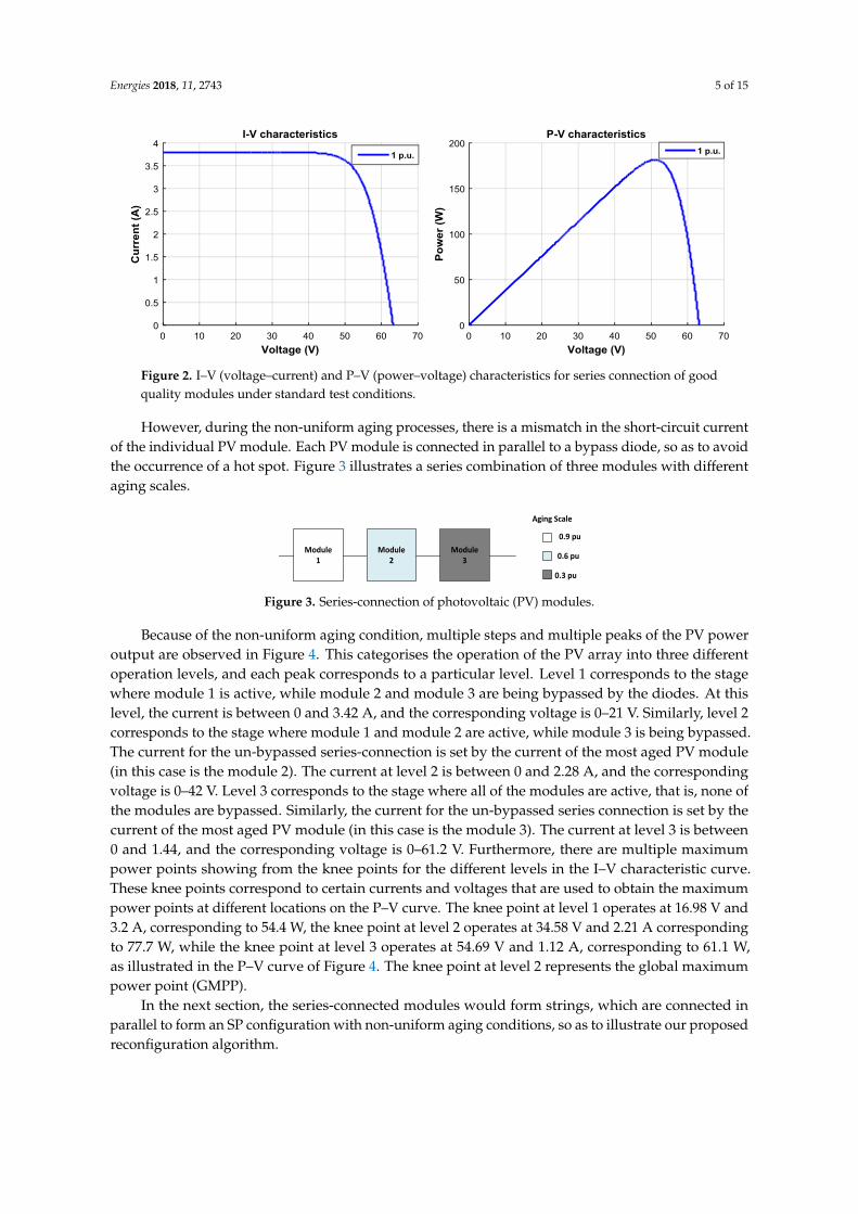
Equations (3) and (4) are true when the modules are identical. Under good quality conditions,the three modules act identically and the voltages of the three modules are equal to a value of 63 V,as shown in Figure 2. Also, as the PV modules are identical, the same short-circuit current flowsthrough the series-connected PV modules, which is equal to 3.74 A (see Figure 2).

Energies 2018, 11, 2743 5 of 15

Energies 2018, 11, x FOR PEER REVIEW 5 of 15

Equations (3) and (4) are true when the modules are identical. Under good quality conditions,

the three modules act identically and the voltages of the three modules are equal to a value of 63 V,

as shown in Figure 2. Also, as the PV modules are identical, the same short-circuit current flows

through the series-connected PV modules, which is equal to 3.74 A (see Figure 2).

Figure 2. I–V (voltage–current) and P–V (power–voltage) characteristics for series connection of good

quality modules under standard test conditions.

However, during the non-uniform aging processes, there is a mismatch in the short-circuit

current of the individual PV module. Each PV module is connected in parallel to a bypass diode, so

as to avoid the occurrence of a hot spot. Figure 3 illustrates a series combination of three modules

with different aging scales.

Module3

Module2

Module1

Aging Scale

0.9 pu

0.6 pu

0.3 pu

Figure 3. Series-connection of photovoltaic (PV) modules.

Because of the non-uniform aging condition, multiple steps and multiple peaks of the PV power

output are observed in Figure 4. This categorises the operation of the PV array into three different

operation levels, and each peak corresponds to a particular level. Level 1 corresponds to the stage

where module 1 is active, while module 2 and module 3 are being bypassed by the diodes. At this

level, the current is between 0 and 3.42 A, and the corresponding voltage is 0–21 V. Similarly, level

2 corresponds to the stage where module 1 and module 2 are active, while module 3 is being

bypassed. The current for the un-bypassed series-connection is set by the current of the most aged

PV module (in this case is the module 2). The current at level 2 is between 0 and 2.28 A, and the

corresponding voltage is 0–42 V. Level 3 corresponds to the stage where all of the modules are active,

that is, none of the modules are bypassed. Similarly, the current for the un-bypassed series connection

is set by the current of the most aged PV module (in this case is the module 3). The current at level 3

is between 0 and 1.44, and the corresponding voltage is 0–61.2 V. Furthermore, there are multiple

maximum power points showing from the knee points for the different levels in the I − V

characteristic curve. These knee points correspond to certain currents and voltages that are used to

obtain the maximum power points at different locations on the P − V curve. The knee point at level

1 operates at 16.98 V and 3.2 A, corresponding to 54.4 W, the knee point at level 2 operates at 34.58 V

and 2.21 A corresponding to 77.7 W, while the knee point at level 3 operates at 54.69 V and 1.12 A,

corresponding to 61.1 W, as illustrated in the P − V curve of Figure 4. The knee point at level 2

represents the global maximum power point (GMPP).

Figure 2. I–V (voltage–current) and P–V (power–voltage) characteristics for series connection of goodquality modules under standard test conditions.

However, during the non-uniform aging processes, there is a mismatch in the short-circuit currentof the individual PV module. Each PV module is connected in parallel to a bypass diode, so as to avoidthe occurrence of a hot spot. Figure 3 illustrates a series combination of three modules with differentaging scales.


Equations (3) and (4) are true when the modules are identical. Under good quality conditions,

the three modules act identically and the voltages of the three modules are equal to a value of 63 V,

as shown in Figure 2. Also, as the PV modules are identical, the same short-circuit current flows

through the series-connected PV modules, which is equal to 3.74 A (see Figure 2).

Figure 2. I–V (voltage–current) and P–V (power–voltage) characteristics for series connection of good

quality modules under standard test conditions.

However, during the non-uniform aging processes, there is a mismatch in the short-circuit

current of the individual PV module. Each PV module is connected in parallel to a bypass diode, so

as to avoid the occurrence of a hot spot. Figure 3 illustrates a series combination of three modules

with different aging scales.

Module3

Module2

Module1

Aging Scale

0.9 pu

0.6 pu

0.3 pu


Because of the non-uniform aging condition, multiple steps and multiple peaks of the PV power

output are observed in Figure 4. This categorises the operation of the PV array into three different

operation levels, and each peak corresponds to a particular level. Level 1 corresponds to the stage

where module 1 is active, while module 2 and module 3 are being bypassed by the diodes. At this

level, the current is between 0 and 3.42 A, and the corresponding voltage is 0–21 V. Similarly, level

2 corresponds to the stage where module 1 and module 2 are active, while module 3 is being

bypassed. The current for the un-bypassed series-connection is set by the current of the most aged

PV module (in this case is the module 2). The current at level 2 is between 0 and 2.28 A, and the

corresponding voltage is 0–42 V. Level 3 corresponds to the stage where all of the modules are active,

that is, none of the modules are bypassed. Similarly, the current for the un-bypassed series connection

is set by the current of the most aged PV module (in this case is the module 3). The current at level 3

is between 0 and 1.44, and the corresponding voltage is 0–61.2 V. Furthermore, there are multiple

maximum power points showing from the knee points for the different levels in the I − V

characteristic curve. These knee points correspond to certain currents and voltages that are used to

obtain the maximum power points at different locations on the P − V curve. The knee point at level

1 operates at 16.98 V and 3.2 A, corresponding to 54.4 W, the knee point at level 2 operates at 34.58 V

and 2.21 A corresponding to 77.7 W, while the knee point at level 3 operates at 54.69 V and 1.12 A,

corresponding to 61.1 W, as illustrated in the P − V curve of Figure 4. The knee point at level 2

represents the global maximum power point (GMPP).


Because of the non-uniform aging condition, multiple steps and multiple peaks of the PV poweroutput are observed in Figure 4. This categorises the operation of the PV array into three differentoperation levels, and each peak corresponds to a particular level. Level 1 corresponds to the stagewhere module 1 is active, while module 2 and module 3 are being bypassed by the diodes. At thislevel, the current is between 0 and 3.42 A, and the corresponding voltage is 0–21 V. Similarly, level 2corresponds to the stage where module 1 and module 2 are active, while module 3 is being bypassed.The current for the un-bypassed series-connection is set by the current of the most aged PV module(in this case is the module 2). The current at level 2 is between 0 and 2.28 A, and the correspondingvoltage is 0–42 V. Level 3 corresponds to the stage where all of the modules are active, that is, none ofthe modules are bypassed. Similarly, the current for the un-bypassed series connection is set by thecurrent of the most aged PV module (in this case is the module 3). The current at level 3 is between0 and 1.44, and the corresponding voltage is 0–61.2 V. Furthermore, there are multiple maximumpower points showing from the knee points for the different levels in the I–V characteristic curve.These knee points correspond to certain currents and voltages that are used to obtain the maximumpower points at different locations on the P–V curve. The knee point at level 1 operates at 16.98 V and3.2 A, corresponding to 54.4 W, the knee point at level 2 operates at 34.58 V and 2.21 A correspondingto 77.7 W, while the knee point at level 3 operates at 54.69 V and 1.12 A, corresponding to 61.1 W,as illustrated in the P–V curve of Figure 4. The knee point at level 2 represents the global maximumpower point (GMPP).

In the next section, the series-connected modules would form strings, which are connected inparallel to form an SP configuration with non-uniform aging conditions, so as to illustrate our proposedreconfiguration algorithm.

Energies 2018, 11, 2743 6 of 15Energies 2018, 11, x FOR PEER REVIEW 6 of 15

Knee point

(GMPP)

Level 1

Level 2

Level 3

77.7 W

Figure 4. I–V and P–V characteristics for series connection under non-uniform aging condition.

In the next section, the series-connected modules would form strings, which are connected in

parallel to form an SP configuration with non-uniform aging conditions, so as to illustrate our

proposed reconfiguration algorithm.

3. PV Array Reconfiguration Scheme

In an N × M PV array, N is the parallel-connected strings and M is the number of series-

connected PV modules, as shown in Figure 5. It is worth noting that the voltage where the GMPP of

a PV array is located in the P − V curve represents the number of active modules for a given string

voltage. Therefore, the maximum power of the PV array is obtained by the product of the sum of all

of the string currents and the string voltage of the active modules.

M

N

Varray

Istring1

Istring2

Istringn

Figure 5. An N × M (parallel-connected strings × number of series-connected PV modules) (PV

array (series parallel (SP) configuration).

A PV array consisting of 16 aged modules connected in a 4 × 4 SP configuration, shown in

Figure 6, will be used to illustrate this concept.

0.8 pu

0.7 pu

0.9 pu

0.5 pu

0.6 pu

0.4 pu

0.9 pu

0.7 pu

0.8 pu

0.5 pu

0.6 pu

0.5 pu

0.8 pu

0.6 pu

0.5 pu

0.4 pu

String 1

String 2

String 3

String 4

Figure 6. A 4 × 4 SP configuration with non-uniform aging.



In an N×M PV array, N is the parallel-connected strings and M is the number of series-connectedPV modules, as shown in Figure 5. It is worth noting that the voltage where the GMPP of a PV array islocated in the P–V curve represents the number of active modules for a given string voltage. Therefore,the maximum power of the PV array is obtained by the product of the sum of all of the string currentsand the string voltage of the active modules.


Knee point

(GMPP)

Level 1

Level 2

Level 3

77.7 W











M

N

Varray

Istring1

Istring2

Istringn





0.8 pu

0.7 pu

0.9 pu

0.5 pu

0.6 pu

0.4 pu

0.9 pu

0.7 pu

0.8 pu

0.5 pu

0.6 pu

0.5 pu

0.8 pu

0.6 pu

0.5 pu

0.4 pu

String 1

String 2

String 3

String 4

Figure 6. A 4 × 4 SP configuration with non-uniform aging.

Figure 5. An N×M (parallel-connected strings × number of series-connected PV modules) (PV array(series parallel (SP) configuration).

A PV array consisting of 16 aged modules connected in a 4 × 4 SP configuration, shown inFigure 6, will be used to illustrate this concept.


Knee point

(GMPP)

Level 1

Level 2

Level 3

77.7 W











M

N

Varray

Istring1

Istring2

Istringn





0.8 pu

0.7 pu

0.9 pu

0.5 pu

0.6 pu

0.4 pu

0.9 pu

0.7 pu

0.8 pu

0.5 pu

0.6 pu

0.5 pu

0.8 pu

0.6 pu

0.5 pu

0.4 pu

String 1

String 2

String 3

String 4

Figure 6. A 4 × 4 SP configuration with non-uniform aging. Figure 6. A 4 × 4 SP configuration with non-uniform aging.

Energies 2018, 11, 2743 7 of 15

In Figure 6, there are four parallel-connected strings (rows) and four series-connected modules(columns), while the per-unit values denote the non-uniform aging status in the PV array, which hasa direct relationship to their individual short-circuit currents.

PV Reconfiguration Algorithm

Generally, the possible number of arrangements for an N × M PV array is(NMM

)(NM−M

M

)(NM− 2M

M

)(NM− 3M

M

)· · ·(

2MM

)(MM

)/N!. For the 4 × 4

PV array, there will be 2,627,625 possible arrangements, and calculating the maximum power for all ofthe possible PV module arrangements for a large PV array (say larger values of N and M) becomesvery difficult. The proposed reconfiguration algorithm is based on an iterative and hierarchical sortingof PV modules, in order to achieve optimum configuration within several iterative steps. In theproposed algorithm, the aging scale (coefficient) shall be used as the varying parameter, as it is directlyrelated to the short-circuit current of each individual PV module. The short-circuit current in a healthymodule is set as 1 p.u. under the standard testing condition (STC), which represents 1000 W/m2

irradiance and 25 C module temperature. The digits in the array represent the different aging factorsof the PV modules, which has a direct relationship to their individual short-circuit currents. Let’sconsider a 4× 4 PV array configuration, shown in Figure 6.

The working parameter shall be the aging factor (AF), which has already been expressed as perunit (p.u.) value of the health status of the individual PV module.

The following parameters are defined in order to outline our proposed algorithm in six steps.

For n = 1, 2, 3, . . . , N − 1, N, where N is the number of strings in the PV array.∑ AFstring n = sum of aging factors in a series-connected string.Mmin(n) = minimum aging factor in a series-connected modules for string n.Pmin = position of PV module with minimum aging factor in a series-connected modules.Mmax(n+1) = maximum aging factor in a series-connected modules for string n + 1.Pmax = position of PV module with maximum aging factor in a series-connected modules.

Step 1: Obtain the summation of AFs for each string, as follows:

∑ AFstring 1 = 0.8 + 0.7 + 0.9 + 0.5 = 2.9 (5)

∑ AFstring 2 = 0.6 + 0.4 + 0.9 + 0.7 = 2.6 (6)

∑ AFstring 3 = 0.8 + 0.5 + 0.6 + 0.5 = 2.4 (7)

∑ AFstring 4 = 0.8 + 0.6 + 0.5 + 0.4 = 2.3 (8)


In Figure 6, there are four parallel-connected strings (rows) and four series-connected modules

(columns), while the per-unit values denote the non-uniform aging status in the PV array, which has

a direct relationship to their individual short-circuit currents.

PV Reconfiguration Algorithm

Generally, the possible number of arrangements for an N × M PV array is

(NMM

)(NM−MM

)(NM−2MM

)(NM−3MM

) ⋯ (2MM

)(MM

)/N!. For the 4 × 4 PV array, there will be 2,627,625 possible

arrangements, and calculating the maximum power for all of the possible PV module arrangements

for a large PV array (say larger values of N and M ) becomes very difficult. The proposed

reconfiguration algorithm is based on an iterative and hierarchical sorting of PV modules, in order to

achieve optimum configuration within several iterative steps. In the proposed algorithm, the aging

scale (coefficient) shall be used as the varying parameter, as it is directly related to the short-circuit

current of each individual PV module. The short-circuit current in a healthy module is set as 1 p.u.

under the standard testing condition (STC), which represents 1000 W/m2 irradiance and 25 °C module

temperature. The digits in the array represent the different aging factors of the PV modules, which

has a direct relationship to their individual short-circuit currents. Let’s consider a 4 × 4 PV array

configuration, shown in Figure 6.

The working parameter shall be the aging factor (AF), which has already been expressed as per

unit (p.u.) value of the health status of the individual PV module.

The following parameters are defined in order to outline our proposed algorithm in six steps.

For n = 1, 2, 3, …, N − 1, N, where N is the number of strings in the PV array.

∑ 𝐴𝐹𝑠𝑡𝑟𝑖𝑛𝑔 𝑛 = sum of aging factors in a series-connected string.

𝑀min(𝑛) = minimum aging factor in a series-connected modules for string n.

𝑃𝑚𝑖𝑛 = position of PV module with minimum aging factor in a series-connected modules.

𝑀max (𝑛+1) = maximum aging factor in a series-connected modules for string n + 1.

𝑃𝑚𝑎𝑥 = position of PV module with maximum aging factor in a series-connected modules.

Step 1: Obtain the summation of AFs for each string, as follows:

∑ 𝐴𝐹𝑠𝑡𝑟𝑖𝑛𝑔 1 = 0.8 + 0.7 + 0.9 + 0.5 = 2.9 (5)

∑ 𝐴𝐹𝑠𝑡𝑟𝑖𝑛𝑔 2 = 0.6 + 0.4 + 0.9 + 0.7 = 2.6 (6)

∑ 𝐴𝐹𝑠𝑡𝑟𝑖𝑛𝑔 3 = 0.8 + 0.5 + 0.6 + 0.5 = 2.4 (7)

∑ 𝐴𝐹𝑠𝑡𝑟𝑖𝑛𝑔 4 = 0.8 + 0.6 + 0.5 + 0.4 = 2.3 (8)

0.8 pu 0.7 pu

0.6 pu

0.8 pu

0.8 pu

2.9 pu

2.6 pu

2.4 pu

2.3 pu

0.4 pu

0.5 pu

0.6 pu

0.9 pu

0.9 pu

0.6 pu

0.5 pu

0.5 pu

0.7 pu

0.5 pu

0.4 pu

Step 2: Arrange the total string level AFs in a descending order, in the case study.

Step 3: Identify 𝑀min(𝑛) and 𝑀max (𝑛+1) for n = 1. Step 2: Arrange the total string level AFs in a descending order, in the case study.Step 3: Identify Mmin(n) and Mmax(n+1) for n = 1.

Energies 2018, 11, 2743 8 of 15


0.8 pu 0.7 pu

0.6 pu

0.8 pu

0.8 pu

2.9 pu

2.6 pu

2.4 pu

2.3 pu

0.4 pu

0.5 pu

0.6 pu

0.9 pu

0.9 pu

0.6 pu

0.5 pu

0.5 pu

0.7 pu

0.5 pu

0.4 pu

𝑀min(1) = 0.5 (9)

𝑀max (2) = 0.9 (10)

If 𝑀min(1) < 𝑀max (2), then swap 𝑃𝑚𝑖𝑛 with 𝑃𝑚𝑎𝑥 and repeat Steps 1, 2, and 3.

0.8 pu 0.7 pu

0.6 pu

0.8 pu

0.8 pu

3.3 pu

2.2 pu

2.4 pu

2.3 pu

0.4 pu

0.5 pu

0.6 pu

0.9 pu

0.5 pu

0.6 pu

0.5 pu

0.9 pu

0.7 pu

0.5 pu

0.4 pu

0.8 pu 0.7 pu

0.8 pu

0.8 pu

0.6 pu

3.3 pu

2.4 pu

2.3 pu

2.2 pu

0.5 pu

0.6 pu

0.4 pu

0.9 pu

0.6 pu

0.5 pu

0.5 pu

0.9 pu

0.5 pu

0.4 pu

0.7 pu

Step 4: Repeat Steps 1, 2, and 3 until 𝑀min(𝑛) ≥ 𝑀max (𝑛+1).

0.8 pu 0.8 pu

0.7 pu

0.8 pu

0.6 pu

3.4 pu

2.3 pu

2.3 pu

2.2 pu

0.5 pu

0.6 pu

0.4 pu

0.9 pu

0.6 pu

0.5 pu

0.5 pu

0.9 pu

0.5 pu

0.4 pu

0.7 pu

0.8 pu 0.7 pu

0.8 pu

0.8 pu

0.6 pu

3.3 pu

2.4 pu

2.3 pu

2.2 pu

0.5 pu

0.6 pu

0.4 pu

0.9 pu

0.6 pu

0.5 pu

0.5 pu

0.9 pu

0.5 pu

0.4 pu

0.7 pu

Step 5: Identify 𝑀min(𝑛) and 𝑀max (𝑛+1) for n = 2, swap the corresponding 𝑃𝑚𝑖𝑛 with 𝑃𝑚𝑎𝑥, and

repeat steps 1, 2, 3, and 4.

0.8 pu 0.8 pu

0.7 pu

0.6 pu

0.5 pu

3.4 pu

2.6 pu

2.2 pu

2.0 pu

0.8 pu

0.4 pu

0.6 pu

0.9 pu

0.6 pu

0.5 pu

0.5 pu

0.9 pu

0.5 pu

0.7 pu

0.4 pu

0.8 pu 0.8 pu

0.7 pu

0.8 pu

0.6 pu

3.4 pu

2.3 pu

2.3 pu

2.2 pu

0.5 pu

0.6 pu

0.4 pu

0.9 pu

0.6 pu

0.5 pu

0.5 pu

0.9 pu

0.5 pu

0.4 pu

0.7 pu

0.8 pu 0.8 pu

0.7 pu

0.6 pu

0.5 pu

3.4 pu

2.8 pu

2.0 pu

2.0 pu

0.8 pu

0.4 pu

0.6 pu

0.9 pu

0.6 pu

0.5 pu

0.5 pu

0.9 pu

0.7 pu

0.5 pu

0.4 pu

0.8 pu 0.8 pu

0.7 pu

0.6 pu

0.5 pu

3.4 pu

2.6 pu

2.2 pu

2.0 pu

0.8 pu

0.4 pu

0.6 pu

0.9 pu

0.6 pu

0.5 pu

0.5 pu

0.9 pu

0.5 pu

0.7 pu

0.4 pu

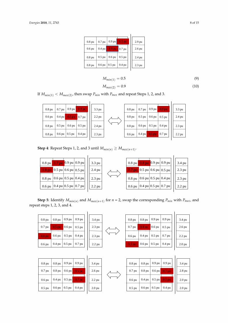
Mmin(1) = 0.5 (9)

Mmax(2) = 0.9 (10)

If Mmin(1) < Mmax(2), then swap Pmin with Pmax and repeat Steps 1, 2, and 3.


0.8 pu 0.7 pu

0.6 pu

0.8 pu

0.8 pu

2.9 pu

2.6 pu

2.4 pu

2.3 pu

0.4 pu

0.5 pu

0.6 pu

0.9 pu

0.9 pu

0.6 pu

0.5 pu

0.5 pu

0.7 pu

0.5 pu

0.4 pu

𝑀min(1) = 0.5 (9)

𝑀max (2) = 0.9 (10)


0.8 pu 0.7 pu

0.6 pu

0.8 pu

0.8 pu

3.3 pu

2.2 pu

2.4 pu

2.3 pu

0.4 pu

0.5 pu

0.6 pu

0.9 pu

0.5 pu

0.6 pu

0.5 pu

0.9 pu

0.7 pu

0.5 pu

0.4 pu

0.8 pu 0.7 pu

0.8 pu

0.8 pu

0.6 pu

3.3 pu

2.4 pu

2.3 pu

2.2 pu

0.5 pu

0.6 pu

0.4 pu

0.9 pu

0.6 pu

0.5 pu

0.5 pu

0.9 pu

0.5 pu

0.4 pu

0.7 pu


0.8 pu 0.8 pu

0.7 pu

0.8 pu

0.6 pu

3.4 pu

2.3 pu

2.3 pu

2.2 pu

0.5 pu

0.6 pu

0.4 pu

0.9 pu

0.6 pu

0.5 pu

0.5 pu

0.9 pu

0.5 pu

0.4 pu

0.7 pu

0.8 pu 0.7 pu

0.8 pu

0.8 pu

0.6 pu

3.3 pu

2.4 pu

2.3 pu

2.2 pu

0.5 pu

0.6 pu

0.4 pu

0.9 pu

0.6 pu

0.5 pu

0.5 pu

0.9 pu

0.5 pu

0.4 pu

0.7 pu



0.8 pu 0.8 pu

0.7 pu

0.6 pu

0.5 pu

3.4 pu

2.6 pu

2.2 pu

2.0 pu

0.8 pu

0.4 pu

0.6 pu

0.9 pu

0.6 pu

0.5 pu

0.5 pu

0.9 pu

0.5 pu

0.7 pu

0.4 pu

0.8 pu 0.8 pu

0.7 pu

0.8 pu

0.6 pu

3.4 pu

2.3 pu

2.3 pu

2.2 pu

0.5 pu

0.6 pu

0.4 pu

0.9 pu

0.6 pu

0.5 pu

0.5 pu

0.9 pu

0.5 pu

0.4 pu

0.7 pu

0.8 pu 0.8 pu

0.7 pu

0.6 pu

0.5 pu

3.4 pu

2.8 pu

2.0 pu

2.0 pu

0.8 pu

0.4 pu

0.6 pu

0.9 pu

0.6 pu

0.5 pu

0.5 pu

0.9 pu

0.7 pu

0.5 pu

0.4 pu

0.8 pu 0.8 pu

0.7 pu

0.6 pu

0.5 pu

3.4 pu

2.6 pu

2.2 pu

2.0 pu

0.8 pu

0.4 pu

0.6 pu

0.9 pu

0.6 pu

0.5 pu

0.5 pu

0.9 pu

0.5 pu

0.7 pu

0.4 pu

Step 4: Repeat Steps 1, 2, and 3 until Mmin(n) ≥ Mmax(n+1).


0.8 pu 0.7 pu

0.6 pu

0.8 pu

0.8 pu

2.9 pu

2.6 pu

2.4 pu

2.3 pu

0.4 pu

0.5 pu

0.6 pu

0.9 pu

0.9 pu

0.6 pu

0.5 pu

0.5 pu

0.7 pu

0.5 pu

0.4 pu

𝑀min(1) = 0.5 (9)

𝑀max (2) = 0.9 (10)


0.8 pu 0.7 pu

0.6 pu

0.8 pu

0.8 pu

3.3 pu

2.2 pu

2.4 pu

2.3 pu

0.4 pu

0.5 pu

0.6 pu

0.9 pu

0.5 pu

0.6 pu

0.5 pu

0.9 pu

0.7 pu

0.5 pu

0.4 pu

0.8 pu 0.7 pu

0.8 pu

0.8 pu

0.6 pu

3.3 pu

2.4 pu

2.3 pu

2.2 pu

0.5 pu

0.6 pu

0.4 pu

0.9 pu

0.6 pu

0.5 pu

0.5 pu

0.9 pu

0.5 pu

0.4 pu

0.7 pu


0.8 pu 0.8 pu

0.7 pu

0.8 pu

0.6 pu

3.4 pu

2.3 pu

2.3 pu

2.2 pu

0.5 pu

0.6 pu

0.4 pu

0.9 pu

0.6 pu

0.5 pu

0.5 pu

0.9 pu

0.5 pu

0.4 pu

0.7 pu

0.8 pu 0.7 pu

0.8 pu

0.8 pu

0.6 pu

3.3 pu

2.4 pu

2.3 pu

2.2 pu

0.5 pu

0.6 pu

0.4 pu

0.9 pu

0.6 pu

0.5 pu

0.5 pu

0.9 pu

0.5 pu

0.4 pu

0.7 pu



0.8 pu 0.8 pu

0.7 pu

0.6 pu

0.5 pu

3.4 pu

2.6 pu

2.2 pu

2.0 pu

0.8 pu

0.4 pu

0.6 pu

0.9 pu

0.6 pu

0.5 pu

0.5 pu

0.9 pu

0.5 pu

0.7 pu

0.4 pu

0.8 pu 0.8 pu

0.7 pu

0.8 pu

0.6 pu

3.4 pu

2.3 pu

2.3 pu

2.2 pu

0.5 pu

0.6 pu

0.4 pu

0.9 pu

0.6 pu

0.5 pu

0.5 pu

0.9 pu

0.5 pu

0.4 pu

0.7 pu

0.8 pu 0.8 pu

0.7 pu

0.6 pu

0.5 pu

3.4 pu

2.8 pu

2.0 pu

2.0 pu

0.8 pu

0.4 pu

0.6 pu

0.9 pu

0.6 pu

0.5 pu

0.5 pu

0.9 pu

0.7 pu

0.5 pu

0.4 pu

0.8 pu 0.8 pu

0.7 pu

0.6 pu

0.5 pu

3.4 pu

2.6 pu

2.2 pu

2.0 pu

0.8 pu

0.4 pu

0.6 pu

0.9 pu

0.6 pu

0.5 pu

0.5 pu

0.9 pu

0.5 pu

0.7 pu

0.4 pu

Step 5: Identify Mmin(n) and Mmax(n+1) for n = 2, swap the corresponding Pmin with Pmax, andrepeat steps 1, 2, 3, and 4.


0.8 pu 0.7 pu

0.6 pu

0.8 pu

0.8 pu

2.9 pu

2.6 pu

2.4 pu

2.3 pu

0.4 pu

0.5 pu

0.6 pu

0.9 pu

0.9 pu

0.6 pu

0.5 pu

0.5 pu

0.7 pu

0.5 pu

0.4 pu

𝑀min(1) = 0.5 (9)

𝑀max (2) = 0.9 (10)


0.8 pu 0.7 pu

0.6 pu

0.8 pu

0.8 pu

3.3 pu

2.2 pu

2.4 pu

2.3 pu

0.4 pu

0.5 pu

0.6 pu

0.9 pu

0.5 pu

0.6 pu

0.5 pu

0.9 pu

0.7 pu

0.5 pu

0.4 pu

0.8 pu 0.7 pu

0.8 pu

0.8 pu

0.6 pu

3.3 pu

2.4 pu

2.3 pu

2.2 pu

0.5 pu

0.6 pu

0.4 pu

0.9 pu

0.6 pu

0.5 pu

0.5 pu

0.9 pu

0.5 pu

0.4 pu

0.7 pu


0.8 pu 0.8 pu

0.7 pu

0.8 pu

0.6 pu

3.4 pu

2.3 pu

2.3 pu

2.2 pu

0.5 pu

0.6 pu

0.4 pu

0.9 pu

0.6 pu

0.5 pu

0.5 pu

0.9 pu

0.5 pu

0.4 pu

0.7 pu

0.8 pu 0.7 pu

0.8 pu

0.8 pu

0.6 pu

3.3 pu

2.4 pu

2.3 pu

2.2 pu

0.5 pu

0.6 pu

0.4 pu

0.9 pu

0.6 pu

0.5 pu

0.5 pu

0.9 pu

0.5 pu

0.4 pu

0.7 pu



0.8 pu 0.8 pu

0.7 pu

0.6 pu

0.5 pu

3.4 pu

2.6 pu

2.2 pu

2.0 pu

0.8 pu

0.4 pu

0.6 pu

0.9 pu

0.6 pu

0.5 pu

0.5 pu

0.9 pu

0.5 pu

0.7 pu

0.4 pu

0.8 pu 0.8 pu

0.7 pu

0.8 pu

0.6 pu

3.4 pu

2.3 pu

2.3 pu

2.2 pu

0.5 pu

0.6 pu

0.4 pu

0.9 pu

0.6 pu

0.5 pu

0.5 pu

0.9 pu

0.5 pu

0.4 pu

0.7 pu

0.8 pu 0.8 pu

0.7 pu

0.6 pu

0.5 pu

3.4 pu

2.8 pu

2.0 pu

2.0 pu

0.8 pu

0.4 pu

0.6 pu

0.9 pu

0.6 pu

0.5 pu

0.5 pu

0.9 pu

0.7 pu

0.5 pu

0.4 pu

0.8 pu 0.8 pu

0.7 pu

0.6 pu

0.5 pu

3.4 pu

2.6 pu

2.2 pu

2.0 pu

0.8 pu

0.4 pu

0.6 pu

0.9 pu

0.6 pu

0.5 pu

0.5 pu

0.9 pu

0.5 pu

0.7 pu

0.4 pu


0.8 pu 0.7 pu

0.6 pu

0.8 pu

0.8 pu

2.9 pu

2.6 pu

2.4 pu

2.3 pu

0.4 pu

0.5 pu

0.6 pu

0.9 pu

0.9 pu

0.6 pu

0.5 pu

0.5 pu

0.7 pu

0.5 pu

0.4 pu

𝑀min(1) = 0.5 (9)

𝑀max (2) = 0.9 (10)


0.8 pu 0.7 pu

0.6 pu

0.8 pu

0.8 pu

3.3 pu

2.2 pu

2.4 pu

2.3 pu

0.4 pu

0.5 pu

0.6 pu

0.9 pu

0.5 pu

0.6 pu

0.5 pu

0.9 pu

0.7 pu

0.5 pu

0.4 pu

0.8 pu 0.7 pu

0.8 pu

0.8 pu

0.6 pu

3.3 pu

2.4 pu

2.3 pu

2.2 pu

0.5 pu

0.6 pu

0.4 pu

0.9 pu

0.6 pu

0.5 pu

0.5 pu

0.9 pu

0.5 pu

0.4 pu

0.7 pu


0.8 pu 0.8 pu

0.7 pu

0.8 pu

0.6 pu

3.4 pu

2.3 pu

2.3 pu

2.2 pu

0.5 pu

0.6 pu

0.4 pu

0.9 pu

0.6 pu

0.5 pu

0.5 pu

0.9 pu

0.5 pu

0.4 pu

0.7 pu

0.8 pu 0.7 pu

0.8 pu

0.8 pu

0.6 pu

3.3 pu

2.4 pu

2.3 pu

2.2 pu

0.5 pu

0.6 pu

0.4 pu

0.9 pu

0.6 pu

0.5 pu

0.5 pu

0.9 pu

0.5 pu

0.4 pu

0.7 pu



0.8 pu 0.8 pu

0.7 pu

0.6 pu

0.5 pu

3.4 pu

2.6 pu

2.2 pu

2.0 pu

0.8 pu

0.4 pu

0.6 pu

0.9 pu

0.6 pu

0.5 pu

0.5 pu

0.9 pu

0.5 pu

0.7 pu

0.4 pu

0.8 pu 0.8 pu

0.7 pu

0.8 pu

0.6 pu

3.4 pu

2.3 pu

2.3 pu

2.2 pu

0.5 pu

0.6 pu

0.4 pu

0.9 pu

0.6 pu

0.5 pu

0.5 pu

0.9 pu

0.5 pu

0.4 pu

0.7 pu

0.8 pu 0.8 pu

0.7 pu

0.6 pu

0.5 pu

3.4 pu

2.8 pu

2.0 pu

2.0 pu

0.8 pu

0.4 pu

0.6 pu

0.9 pu

0.6 pu

0.5 pu

0.5 pu

0.9 pu

0.7 pu

0.5 pu

0.4 pu

0.8 pu 0.8 pu

0.7 pu

0.6 pu

0.5 pu

3.4 pu

2.6 pu

2.2 pu

2.0 pu

0.8 pu

0.4 pu

0.6 pu

0.9 pu

0.6 pu

0.5 pu

0.5 pu

0.9 pu

0.5 pu

0.7 pu

0.4 pu

Energies 2018, 11, 2743 9 of 15

Step 6: Repeat step 5 until the end (N − 1).Energies 2018, 11, x FOR PEER REVIEW 9 of 15

Step 6: Repeat step 5 until the end (N − 1).

0.8 pu 0.8 pu

0.7 pu

0.6 pu

0.5 pu

3.4 pu

2.8 pu

2.2 pu

1.8 pu

0.8 pu

0.6 pu

0.4 pu

0.9 pu

0.6 pu

0.5 pu

0.5 pu

0.9 pu

0.7 pu

0.5 pu

0.4 pu

0.8 pu 0.8 pu

0.7 pu

0.6 pu

0.5 pu

3.4 pu

2.8 pu

2.0 pu

2.0 pu

0.8 pu

0.4 pu

0.6 pu

0.9 pu

0.6 pu

0.5 pu

0.5 pu

0.9 pu

0.7 pu

0.5 pu

0.4 pu

From the last step, the array atthe right hand side (RHS) shows the optimum configuration.

However, each of the configurations that arrived at each step were compared with the original

arrangement, as shown in Figure 6. As illustrated for the 4 × 4 PV array, only six iterative steps were

needed to arrive at the optimum configuration for a non-uniform aging condition. Furthermore, a

MATLAB program is written to execute for a large PV array, and the optimized form depicts the

arrangements for the optimum power output. Therefore, for the instance of a 4 × 4 PV array, the

array “after” arrangement is the optimum configuration. Figure 7 shows the comparison between the

PV array “before” and “after” arrangement.

0.8 pu 0.8 pu

0.7 pu

0.6 pu

0.5 pu

0.8 pu

0.6 pu

0.4 pu

0.9 pu

0.6 pu

0.5 pu

0.5 pu

0.9 pu

0.7 pu

0.5 pu

0.4 pu

0.8 pu 0.7 pu

0.6 pu

0.8 pu

0.8 pu

0.4 pu

0.5 pu

0.6 pu

0.9 pu

0.9 pu

0.6 pu

0.5 pu

0.5 pu

0.7 pu

0.5 pu

0.4 pu

afterbefore

Figure 7. PV Array “before” and “after” rearrangement.

The maximum power and voltage at MPP were tabulated in Table 2 for each configuration and

the string currents in each case. Clearly, the total output power is increased by 22.4% between Step 1

and Step 6. Also, the voltage at MPP does not vary much compared to the output current. This

algorithm maximizes the currents in each string by combining the PV modules with almost the same

electrical characteristics, so as to reduce multiple peaks resulting from mismatch effects (non-uniform

aging).

Table 2. Electrical parameters obtained for different reconfigurations. MPP—maximum power point.

Steps Maximum Power (𝑷𝒎)

(W)

Voltage at MPP (𝑽𝒎)

(V)

String Currents (A)

1 2 3 4

1 468.6 71 1.863 1.492 1.757 1.482

2 515.6 70 2.587 1.793 1.490 1.488

3 530.7 70 2.818 1.779 1.490 1.488

4 535.3 70 2.818 1.859 1.488 1.475

5 558.6 70 2.818 2.206 1.475 1.475

6 573.7 69 2.867 2.260 1.790 1.428

To execute the MATLAB program. the PV array shall be represented in matrix form, given by

Equation (11).

From the last step, the array atthe right hand side (RHS) shows the optimum configuration.However, each of the configurations that arrived at each step were compared with the originalarrangement, as shown in Figure 6. As illustrated for the 4× 4 PV array, only six iterative stepswere needed to arrive at the optimum configuration for a non-uniform aging condition. Furthermore,a MATLAB program is written to execute for a large PV array, and the optimized form depicts thearrangements for the optimum power output. Therefore, for the instance of a 4× 4 PV array, the array“after” arrangement is the optimum configuration. Figure 7 shows the comparison between the PVarray “before” and “after” arrangement.


Step 6: Repeat step 5 until the end (N − 1).

0.8 pu 0.8 pu

0.7 pu

0.6 pu

0.5 pu

3.4 pu

2.8 pu

2.2 pu

1.8 pu

0.8 pu

0.6 pu

0.4 pu

0.9 pu

0.6 pu

0.5 pu

0.5 pu

0.9 pu

0.7 pu

0.5 pu

0.4 pu

0.8 pu 0.8 pu

0.7 pu

0.6 pu

0.5 pu

3.4 pu

2.8 pu

2.0 pu

2.0 pu

0.8 pu

0.4 pu

0.6 pu

0.9 pu

0.6 pu

0.5 pu

0.5 pu

0.9 pu

0.7 pu

0.5 pu

0.4 pu

From the last step, the array atthe right hand side (RHS) shows the optimum configuration.

However, each of the configurations that arrived at each step were compared with the original

arrangement, as shown in Figure 6. As illustrated for the 4 × 4 PV array, only six iterative steps were

needed to arrive at the optimum configuration for a non-uniform aging condition. Furthermore, a

MATLAB program is written to execute for a large PV array, and the optimized form depicts the

arrangements for the optimum power output. Therefore, for the instance of a 4 × 4 PV array, the

array “after” arrangement is the optimum configuration. Figure 7 shows the comparison between the

PV array “before” and “after” arrangement.

0.8 pu 0.8 pu

0.7 pu

0.6 pu

0.5 pu

0.8 pu

0.6 pu

0.4 pu

0.9 pu

0.6 pu

0.5 pu

0.5 pu

0.9 pu

0.7 pu

0.5 pu

0.4 pu

0.8 pu 0.7 pu

0.6 pu

0.8 pu

0.8 pu

0.4 pu

0.5 pu

0.6 pu

0.9 pu

0.9 pu

0.6 pu

0.5 pu

0.5 pu

0.7 pu

0.5 pu

0.4 pu

afterbefore


The maximum power and voltage at MPP were tabulated in Table 2 for each configuration and

the string currents in each case. Clearly, the total output power is increased by 22.4% between Step 1

and Step 6. Also, the voltage at MPP does not vary much compared to the output current. This

algorithm maximizes the currents in each string by combining the PV modules with almost the same

electrical characteristics, so as to reduce multiple peaks resulting from mismatch effects (non-uniform

aging).


Steps Maximum Power (𝑷𝒎)

(W)

Voltage at MPP (𝑽𝒎)

(V)

String Currents (A)

1 2 3 4

1 468.6 71 1.863 1.492 1.757 1.482

2 515.6 70 2.587 1.793 1.490 1.488

3 530.7 70 2.818 1.779 1.490 1.488

4 535.3 70 2.818 1.859 1.488 1.475

5 558.6 70 2.818 2.206 1.475 1.475

6 573.7 69 2.867 2.260 1.790 1.428

To execute the MATLAB program. the PV array shall be represented in matrix form, given by

Equation (11).


The maximum power and voltage at MPP were tabulated in Table 2 for each configuration and thestring currents in each case. Clearly, the total output power is increased by 22.4% between Step 1 andStep 6. Also, the voltage at MPP does not vary much compared to the output current. This algorithmmaximizes the currents in each string by combining the PV modules with almost the same electricalcharacteristics, so as to reduce multiple peaks resulting from mismatch effects (non-uniform aging).


Steps Maximum Power (Pm)(W)

Voltage at MPP (Vm)(V)

String Currents (A)

1 2 3 4

1 468.6 71 1.863 1.492 1.757 1.4822 515.6 70 2.587 1.793 1.490 1.4883 530.7 70 2.818 1.779 1.490 1.4884 535.3 70 2.818 1.859 1.488 1.4755 558.6 70 2.818 2.206 1.475 1.4756 573.7 69 2.867 2.260 1.790 1.428

To execute the MATLAB program. the PV array shall be represented in matrix form, given byEquation (11).

Energies 2018, 11, 2743 10 of 15

N by Mmatrix =

0.8 0.7 0.9 0.50.6 0.4 0.9 0.70.8 0.5 0.6 0.50.8 0.6 0.5 0.4

(11)

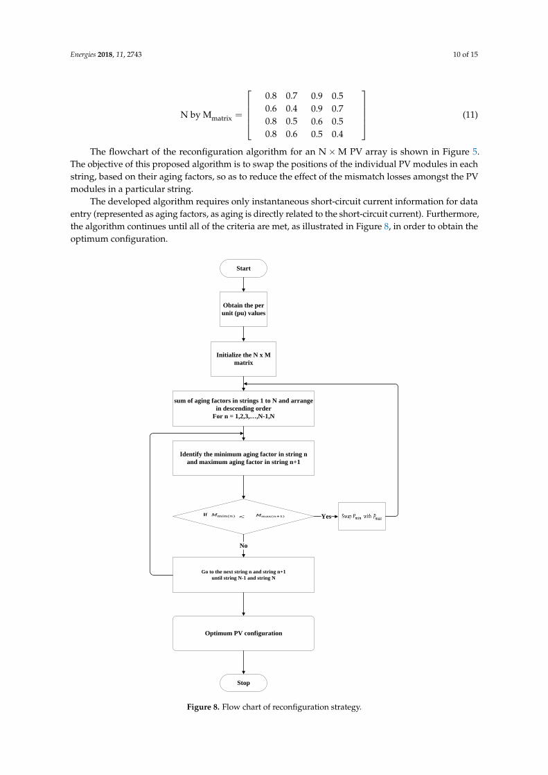
The flowchart of the reconfiguration algorithm for an N×M PV array is shown in Figure 5.The objective of this proposed algorithm is to swap the positions of the individual PV modules in eachstring, based on their aging factors, so as to reduce the effect of the mismatch losses amongst the PVmodules in a particular string.

The developed algorithm requires only instantaneous short-circuit current information for dataentry (represented as aging factors, as aging is directly related to the short-circuit current). Furthermore,the algorithm continues until all of the criteria are met, as illustrated in Figure 8, in order to obtain theoptimum configuration.


N by Mmatrix = [

0.8 0.7 0.9 0.50.6 0.4 0.9 0.70.8 0.5 0.6 0.50.8 0.6 0.5 0.4

] (11)

The flowchart of the reconfiguration algorithm for an N × M PV array is shown in Figure 5. The

objective of this proposed algorithm is to swap the positions of the individual PV modules in each

string, based on their aging factors, so as to reduce the effect of the mismatch losses amongst the PV

modules in a particular string.

The developed algorithm requires only instantaneous short-circuit current information for data

entry (represented as aging factors, as aging is directly related to the short-circuit current).

Furthermore, the algorithm continues until all of the criteria are met, as illustrated in Figure 8, in

order to obtain the optimum configuration.

Start

Obtain the per

unit (pu) values

Initialize the N x M

matrix

sum of aging factors in strings 1 to N and arrange

in descending order

For n = 1,2,3, ,N-1,N

Identify the minimum aging factor in string n

and maximum aging factor in string n+1

Go to the next string n and string n+1

until string N-1 and string N

Stop

No

Yes

Optimum PV configuration

Figure 8. Flow chart of reconfiguration strategy. Figure 8. Flow chart of reconfiguration strategy.

Energies 2018, 11, 2743 11 of 15

4. Results and Discussions

4.1. Simulation Results

In order to validate the proposed algorithm, PV arrays of different sizes will be considered, thatis, 4 × 4, 10 × 10, and 100 × 10 PV arrays. The maximum output powers from the PV configurationbefore and after arrangement are obtained using a PV array model built in MATLAB.

A computer with Intel (R) Core (TM) i3-5005U CPU at 2.00 GHz, with 4 G RAM was used toperform the calculation and the corresponding computing time for a 4 × 4, 10 × 10, and 100 × 10 PVarray tabulated.

4.2. Case 1: 4 × 4 PV Array

Figure 6 will be used in this case to verify the results using MATLAB. The maximum short-circuitcurrent in a healthy module is set as 1 p.u. under the standard testing condition (STC), which representsthe 1000 W/m2 irradiance and 25 C module temperature.

In Table 3, the PV configuration after arrangement was obtained using the proposed algorithm.With the information of the PV array shown in Table 3, the I −V and P−V characteristic curves areplotted as shown in Figure 9. Figure 9 shows that the maximum output power before arrangement,which is 468.6 W, and the PV array output voltage and current for the GMPP are 71 V and 6.498 A,respectively. The maximum output power after arrangement is 573.7 W, and the PV array outputvoltage and current for the GMPP are 69 V and 8.255 A, respectively. Obviously, the total output powerincreases by 22.4% when the proposed algorithm is used. The computing time for the rearrangementsof an aged 4 × 4 PV array takes 0.01 s to execute our proposed algorithm as shown in Table 4.

Table 3. PV configuration before and after arrangement for Case 1.

Before Arrangement After Arrangement

0.8 pu 0.7 pu 0.9 pu 0.5 pu 0.8 pu 0.8 pu 0.9 pu 0.9 pu0.6 pu 0.4 pu 0.9 pu 0.7 pu 0.7 pu 0.8 pu 0.6 pu 0.7 pu0.8 pu 0.5 pu 0.6 pu 0.5 pu 0.6 pu 0.6 pu 0.5 pu 0.5 pu0.8 pu 0.6 pu 0.5 pu 0.4 pu 0.5 pu 0.4 pu 0.5 pu 0.4 pu

Table 4. 4 × 4 PV array parameters (before and after arrangement).

Parameter Before After Computing Time (s) Power Improvement (Percentage)

Pm 468.6 W 573.7 W0.01 22.4%Vm 71 V 69 V

Im 6.498 A 8.255 A


4. Results and Discussions

4.1. Simulation Results

In order to validate the proposed algorithm, PV arrays of different sizes will be considered, that

is, 4 × 4, 10 × 10, and 100 × 10 PV arrays. The maximum output powers from the PV configuration

before and after arrangement are obtained using a PV array model built in MATLAB.

A computer with Intel (R) Core (TM) i3-5005U CPU at 2.00 GHz, with 4 G RAM was used to

perform the calculation and the corresponding computing time for a 4 × 4, 10 × 10, and 100 × 10 PV

array tabulated.

4.2. Case 1: 4 × 4 PV Array

Figure 6 will be used in this case to verify the results using MATLAB. The maximum short-

circuit current in a healthy module is set as 1 p.u. under the standard testing condition (STC), which

represents the 1000 W/m2 irradiance and 25 °C module temperature.

In Table 3, the PV configuration after arrangement was obtained using the proposed algorithm.

With the information of the PV array shown in Table 3, the 𝐼 − 𝑉 and 𝑃 − 𝑉 characteristic curves

are plotted as shown in Figure 9. Figure 9 shows that the maximum output power before

arrangement, which is 468.6 W, and the PV array output voltage and current for the GMPP are 71 V

and 6.498 A, respectively. The maximum output power after arrangement is 573.7 W, and the PV

array output voltage and current for the GMPP are 69 V and 8.255 A, respectively. Obviously, the

total output power increases by 22.4% when the proposed algorithm is used. The computing time for

the rearrangements of an aged 4 × 4 PV array takes 0.01 s to execute our proposed algorithm as shown

in Table 4.


Before Arrangement After Arrangement

0.8 pu 0.7 pu 0.9 pu 0.5 pu 0.8 pu 0.8 pu 0.9 pu 0.9 pu






𝑃𝑚 468.6 W 573.7 W 0.01 22.4% 𝑉𝑚 71 V 69 V

𝐼𝑚 6.498 A 8.255 A

Figure 9. The array output (before and after arrangement) for case 1. Figure 9. The array output (before and after arrangement) for case 1.

Energies 2018, 11, 2743 12 of 15

4.3. Case 2: 10 × 10 PV Array

For a medium size 10× 10 PV array, there are 10 parallel-connected strings and 10 series-connectedmodules. Here, the aging factors, ranging from 0.4 p.u. to 0.9 p.u., were randomly generatedin MATLAB (R2015a) to form a 10× 10 matrix, replicating a non-uniform aging PV array beforearrangement, as shown in Table 5, as well as the optimum PV configuration (after arrangement)for this case. These two PV configurations were simulated and the result shows that the proposedalgorithm gives an optimum configuration. Figure 10 shows that the maximum output power beforearrangement is 2754 W, and the PV array output voltage and current for the GMPP are 164 V and16.95 A, respectively. The maximum output power after arrangement is 3920 W, and the PV arrayoutput voltage and current for the GMPP are 171 V and 21.13 A, respectively. The computing time forthe rearrangements of an aged 10× 10 PV array takes 0.035 s to execute in our proposed algorithm asshown in Table 6.


Before Arrangement

0.4 pu 0.6 pu 0.4 pu 0.6 pu 0.9 pu 0.6 pu 0.8 pu 0.5 pu 0.7 pu 0.9 pu0.8 pu 0.4 pu 0.9 pu 0.9 pu 0.7 pu 0.4 pu 0.6 pu 0.6 pu 0.5 pu 0.8 pu0.5 pu 0.5 pu 0.4 pu 0.5 pu 0.6 pu 0.9 pu 0.5 pu 0.8 pu 0.8 pu 0.6 pu0.7 pu 0.9 pu 0.8 pu 0.5 pu 0.7 pu 0.9 pu 0.6 pu 0.4 pu 0.5 pu 0.6 pu0.4 pu 0.4 pu 0.8 pu 0.4 pu 0.6 pu 0.6 pu 0.4 pu 0.4 pu 0.8 pu 0.6 pu0.7 pu 0.8 pu 0.9 pu 0.4 pu 0.4 pu 0.6 pu 0.4 pu 0.5 pu 0.5 pu 0.5 pu0.5 pu 0.7 pu 0.4 pu 0.9 pu 0.5 pu 0.6 pu 0.9 pu 0.7 pu 0.6 pu 0.7 pu0.7 pu 0.9 pu 0.6 pu 0.7 pu 0.4 pu 0.9 pu 0.9 pu 0.8 pu 0.7 pu 0.7 pu0.8 pu 0.4 pu 0.5 pu 0.7 pu 0.5 pu 0.6 pu 0.7 pu 0.7 pu 0.8 pu 0.8 pu0.8 pu 0.6 pu 0.8 pu 0.4 pu 0.5 pu 0.4 pu 0.4 pu 0.6 pu 0.4 pu 0.8 pu

After Arrangement

0.9 pu 0.9 pu 0.9 pu 0.9 pu 0.9 pu 0.9 pu 0.9 pu 0.9 pu 0.9 pu 0.9 pu0.9 pu 0.8 pu 0.8 pu 0.8 pu 0.9 pu 0.9 pu 0.8 pu 0.8 pu 0.8 pu 0.8 pu0.8 pu 0.8 pu 0.8 pu 0.8 pu 0.8 pu 0.8 pu 0.8 pu 0.8 pu 0.7 pu 0.8 pu0.7 pu 0.7 pu 0.7 pu 0.7 pu 0.7 pu 0.7 pu 0.7 pu 0.7 pu 0.7 pu 0.7 pu0.7 pu 0.6 pu 0.6 pu 0.6 pu 0.7 pu 0.6 pu 0.6 pu 0.7 pu 0.7 pu 0.6 pu0.6 pu 0.6 pu 0.6 pu 0.6 pu 0.6 pu 0.6 pu 0.6 pu 0.6 pu 0.6 pu 0.6 pu0.5 pu 0.5 pu 0.5 pu 0.6 pu 0.5 pu 0.6 pu 0.5 pu 0.5 pu 0.5 pu 0.6 pu0.5 pu 0.5 pu 0.5 pu 0.5 pu 0.5 pu 0.5 pu 0.4 pu 0.5 pu 0.5 pu 0.5 pu0.4 pu 0.4 pu 0.4 pu 0.4 pu 0.4 pu 0.4 pu 0.4 pu 0.4 pu 0.4 pu 0.4 pu0.4 pu 0.4 pu 0.4 pu 0.4 pu 0.4 pu 0.4 pu 0.4 pu 0.4 pu 0.4 pu 0.4 puEnergies 2018, 11, x FOR PEER REVIEW 13 of 15

Figure 10. The array output (before and after arrangement) for Case 2.

4.4. Case 3: 100 × 10 PV Array

For a large PV array, say a 100 × 10 array with 100 parallel-connected strings and 10 series-

connected modules. The non-uniform aging factors were randomly generated, as in Case 2. It was

observed that the power improved by 36.7% when the proposed algorithm was applied, and the

average computing time was 2.746 s, as shown in Table 7.



𝑃𝑚 27.69 kW 37.85 kW 2.746 36.7% 𝑉𝑚 165 V 168 V

𝐼𝑚 167 A 223 A

4.5. Discussions

From the results obtained for the three cases, it is observed that the proposed algorithm can be

applicable to different sizes of PV arrays, and an improved maximum power has been achieved for

the three cases. In addition, the proposed algorithm minimizes the effect of the bypass diodes by

swapping the positions of the individual PV modules in each string based on their aging factors, so

as to reduce the effect of mismatch losses amongst PV modules in a particular string, but the voltage

limitation was not considered in this work, as discussed by the authors of [22]. This algorithm

involves a hierarchical and iterative sorting of the PV modules. The P − V curves (see Figures 9–11)

for the three cases show that the effect of mismatch amongst the PV modules has been reduced after

the rearrangement. Moreover, this proposed algorithm does not need to access all of the possible

configurations for a particular PV array (huge number), which makes it relatively faster. For instance,

in Case 1, only six steps were needed for the algorithm to arrive at the optimum arrangement

(configuration) without having to go through all 2,627,625 possible arrangements. The computing

time for the three cases was recorded in Tables Table 4 Table 5 Table 6 Table 7 . In other words, the

optimal configuration with the proposed algorithm can be found in a short time and can in turn be

applied for implementation in real time. Interestingly, the affected PV modules to be swapped are

the only ones involved in the transition, while the rest remain in their original position, therefore

reducing the number of relays to be used for switching purposes, which in turn saves on cost and

time compared with that proposed in refs. [6] and [22].


Energies 2018, 11, 2743 13 of 15



Pm 2754 W 3624 W0.035 31.6%Vm 164 V 171 V

Im 16.95 A 21.13 A

4.4. Case 3: 100 × 10 PV Array

For a large PV array, say a 100 × 10 array with 100 parallel-connected strings and 10 series-connected modules. The non-uniform aging factors were randomly generated, as in Case 2. It wasobserved that the power improved by 36.7% when the proposed algorithm was applied, and theaverage computing time was 2.746 s, as shown in Table 7.



Pm 27.69 kW 37.85 kW2.746 36.7%Vm 165 V 168 V

Im 167 A 223 A

4.5. Discussions

From the results obtained for the three cases, it is observed that the proposed algorithm can beapplicable to different sizes of PV arrays, and an improved maximum power has been achieved for thethree cases. In addition, the proposed algorithm minimizes the effect of the bypass diodes by swappingthe positions of the individual PV modules in each string based on their aging factors, so as to reducethe effect of mismatch losses amongst PV modules in a particular string, but the voltage limitation wasnot considered in this work, as discussed by the authors of [22]. This algorithm involves a hierarchicaland iterative sorting of the PV modules. The P − V curves (see Figures 9–11) for the three casesshow that the effect of mismatch amongst the PV modules has been reduced after the rearrangement.Moreover, this proposed algorithm does not need to access all of the possible configurations fora particular PV array (huge number), which makes it relatively faster. For instance, in Case 1, only sixsteps were needed for the algorithm to arrive at the optimum arrangement (configuration) withouthaving to go through all 2,627,625 possible arrangements. The computing time for the three cases wasrecorded in Tables 4–7. In other words, the optimal configuration with the proposed algorithm can befound in a short time and can in turn be applied for implementation in real time. Interestingly, theaffected PV modules to be swapped are the only ones involved in the transition, while the rest remainin their original position, therefore reducing the number of relays to be used for switching purposes,which in turn saves on cost and time compared with that proposed in refs. [6,22].

Energies 2018, 11, 2743 14 of 15Energies 2018, 11, x FOR PEER REVIEW 14 of 15


5. Conclusions

In this work, we studied and analysed the non-uniform aging processes in the PV arrays, and

we found that the locations of aged PV modules in the PV arrays influence the power generation of

the solar PV arrays. In order to alleviate the negative influence of non-uniformly aging PV arrays, we

propose a novel PV array reconfiguration algorithm to maximize the power generation from non-

uniformly aged PV arrays, without replacing the aged PV modules with new ones. In this algorithm,

the PV modules are sorted iteratively in a hierarchy pattern so as to reduce the effect of mismatch

due to non-uniform aging amongst PV modules, and the maximum power output has improved by

22.4%, 31.6%, and 36.7% for the 4 × 4, 10 × 10, and 100 × 10 arrays, respectively.

Compared to the existing online PV array reconfiguration methods, the proposed PV module

rearrangement approach requires fewer relays but effectively boost the PV systems’ maximum power

output. The proposed algorithm is also easily implementable, as it only requires swapping locations

of the PV modules.

Author Contributions: Conceptualization, P.U. and Y.H.; Methodology, Y.H.; Software, K.N.; Validation, Y.H.

and X.Y.; Formal Analysis, H.W., X.Y.; Investigation, H.W.; Resources, P.U.; Data Curation, P.U.; Writing-

Original Draft Preparation, P.U.; Writing-Review & Editing, X.Y.; Visualization, K.N.; Supervision, Y.H.; Project

Administration, Y.H.; Funding Acquisition, Y.H. and X.Y.

Funding: This study was supported by the Royal Academy of Engineering under the Industry Academia

Partnership Programme—17/18 scheme (Grant number: IAPP1\100015).

Conflicts of Interest: The authors declare no conflicts of interest.

References

1. Sanseverino, E.R.; Ngoc, T.N.; Cardinale, M.; Vigni, V.L.; Musso, D.; Romano, P.; Viola, F. Dynamic

programming and munkres algorithm for optimal pv arrays reconfiguration. Sol. Energy 2015, 122, 347–

358.

2. International Renewable Energy Agency (IRENA), Renewable Power Generation Costs in 2017. Available

online: https://www.irena.org//media/Files/IRENA/Agency/Publication/2018/Jan/IRENA_2017_Power_Co

sts_2018.pdf (accessed on 12 September 2018).

3. Banavar, M.; Braun, H.; Buddha, S.T.; Krishnan, V.; Spanias, A.; Takada, S.; Takehara, T.; Tepedelenlioglu,

C.; Yeider, T. Signal processing for solar array monitoring, fault detection, and optimization. Ynth. Lect.

Power Electron. 2012, 7, 1–95.

4. Photovoltaics Report, Fraunhofer ISE and Werner Warmuth, PSE Conferences & Consulting GmbH, 27th

August, 2018. Available online: hhtps://www.ise.fraunhofer.de (accessed on 12 September 2018).

5. Goodrich, A.; James, T.; Woodhouse, M. Residential, commercial and utility-scale PV system prices in the

US: Current drivers and cost-reduction opportunities. Natl. Renew. Energy Lab. 2012, doi:10.2172/1036048.

6. Hu, Y.; Zhang, J.; Wu, J.; Cao, W.; Tian, G.Y.; Kirtley, J.L. Efficiency of non-uniformly aged PV array. IEEE

Trans. Power Electron. 2017, 32, 1124–1137.


5. Conclusions

In this work, we studied and analysed the non-uniform aging processes in the PV arrays, andwe found that the locations of aged PV modules in the PV arrays influence the power generation ofthe solar PV arrays. In order to alleviate the negative influence of non-uniformly aging PV arrays,we propose a novel PV array reconfiguration algorithm to maximize the power generation fromnon-uniformly aged PV arrays, without replacing the aged PV modules with new ones. In thisalgorithm, the PV modules are sorted iteratively in a hierarchy pattern so as to reduce the effect ofmismatch due to non-uniform aging amongst PV modules, and the maximum power output hasimproved by 22.4%, 31.6%, and 36.7% for the 4 × 4, 10 × 10, and 100 × 10 arrays, respectively.

Compared to the existing online PV array reconfiguration methods, the proposed PV modulerearrangement approach requires fewer relays but effectively boost the PV systems’ maximum poweroutput. The proposed algorithm is also easily implementable, as it only requires swapping locations ofthe PV modules.

Author Contributions: Conceptualization, P.U. and Y.H.; Methodology, Y.H.; Software, K.N.; Validation, Y.H. andX.Y.; Formal Analysis, H.W., X.Y.; Investigation, H.W.; Resources, P.U.; Data Curation, P.U.; Writing-Original DraftPreparation, P.U.; Writing-Review & Editing, X.Y.; Visualization, K.N.; Supervision, Y.H.; Project Administration,Y.H.; Funding Acquisition, Y.H. and X.Y.

Funding: This study was supported by the Royal Academy of Engineering under the Industry AcademiaPartnership Programme—17/18 scheme (Grant number: IAPP1\100015).

Conflicts of Interest: The authors declare no conflicts of interest.

References

1. Sanseverino, E.R.; Ngoc, T.N.; Cardinale, M.; Vigni, V.L.; Musso, D.; Romano, P.; Viola, F. Dynamicprogramming and munkres algorithm for optimal pv arrays reconfiguration. Sol. Energy 2015, 122, 347–358.[CrossRef]

2. International Renewable Energy Agency (IRENA), Renewable Power Generation Costs in 2017. Availableonline: https://www.irena.org//media/Files/IRENA/Agency/Publication/2018/Jan/IRENA_2017_Power_Costs_2018.pdf (accessed on 12 September 2018).

3. Banavar, M.; Braun, H.; Buddha, S.T.; Krishnan, V.; Spanias, A.; Takada, S.; Takehara, T.; Tepedelenlioglu, C.;Yeider, T. Signal processing for solar array monitoring, fault detection, and optimization. Ynth. Lect. PowerElectron. 2012, 7, 1–95. [CrossRef]

4. Photovoltaics Report, Fraunhofer ISE and Werner Warmuth, PSE Conferences & Consulting GmbH,27 August 2018. Available online: hhtps://www.ise.fraunhofer.de (accessed on 12 September 2018).

5. Goodrich, A.; James, T.; Woodhouse, M. Residential, commercial and utility-scale PV system prices in theUS: Current drivers and cost-reduction opportunities. Natl. Renew. Energy Lab. 2012. [CrossRef]

6. Hu, Y.; Zhang, J.; Wu, J.; Cao, W.; Tian, G.Y.; Kirtley, J.L. Efficiency of non-uniformly aged PV array. IEEE Trans.Power Electron. 2017, 32, 1124–1137. [CrossRef]

http://dx.doi.org/10.1016/j.solener.2015.09.016

https://www.irena.org//media/Files/IRENA/Agency/Publication/2018/Jan/IRENA_2017_Power_Costs_2018.pdf

https://www.irena.org//media/Files/IRENA/Agency/Publication/2018/Jan/IRENA_2017_Power_Costs_2018.pdf

http://dx.doi.org/10.2200/S00425ED1V01Y201206PEL004

hhtps://www.ise.fraunhofer.de

http://dx.doi.org/10.2172/1036048

http://dx.doi.org/10.1109/TPEL.2016.2544842

Energies 2018, 11, 2743 15 of 15

7. Ndiaye, A.; Kébé, C.M.; Ndiaye, P.A.; Charki, A.; Kobi, A.; Sambou, V. A novel method for investigatingphotovoltaic module degradation. Energy Procedia 2013, 36, 1222–1231. [CrossRef]

8. Mekhilefa, S.; Saidurb, R.; Kamalisarvestanib, M. Effect of dust, humidity and air velocity on efficiency ofphotovoltaic cells. Renew. Sustain. Energy Rev. 2012, 16, 2920–2925. [CrossRef]

9. Cristaldi, L.; Faifer, M.; Rossi, M.; Toscani, S.; Catelani, M.; Ciani, L.; Lazzaroni, M. Simplified method forevaluating the effects of dust and aging on photovoltaic panels. Measurement 2014, 54, 207–214. [CrossRef]

10. Femia, N.; Petrone, G.; Spagnuolo, G.; Vitelli, M. Power Electronics and Control Techniques for Maximum EnergyHarvesting in Photovoltaic Systems; CRC Press: Boca Raton, FL, USA, 2012.

11. Balato, M.; Costanzo, L.; Vitelli, M. Reconfiguration of PV modules: A tool to get the best compromisebetween maximization of the extracted power and minimization of localized heating phenomena. Sol. Energy2016, 138, 105–118. [CrossRef]

12. Kaplanis, S.; Kaplani, E. Energy performance and degradation over 20 years performance of BP c-Si PVmodules. Simul. Model. Pract. Theory 2011, 19, 1201–1211. [CrossRef]

13. Shirzadi, S.; Hizam, H.; Wahab, N.I.A. Mismatch losses minimization in photovoltaic arrays by arrangingmodules applying a genetic algorithm. Sol. Energy 2014, 108, 467–478. [CrossRef]

14. Manganiello, P.; Balato, M.; Vitelli, M. A survey on mismatching and aging of PV Modules: The closed loop.IEEE Trans. Ind. Electron. 2015, 62, 7276–7286. [CrossRef]

15. La Manna, D.; Vigni, V.L.; Sanseverino, E.R.; Di Dio, V.; Romano, P. Reconfigurable electrical interconnectionstrategies for photovoltaic arrays: A review. Renew. Sustain. Energy Rev. 2014, 33, 412–426. [CrossRef]

16. Malathy, S.; Ramaprabha, R. Comprehensive analysis on the role of array size and configuration on energyyield of photovoltaic systems under shaded conditions. Renew. Sustain. Energy Rev. 2015, 49, 672–679.[CrossRef]

17. Camarillo-Peñaranda, J.R.; Ramírez-Quiroz, F.A.; González-Montoya, D.; Bolaños-Martínez, F.; Ramos-Paja, C.A.Reconfiguration of photovoltaic arrays based on genetic algorithm. Rev. Fac. Ing. Univ. Antioq. 2015, 95–107.[CrossRef]

18. Auttawaitkul, Y.; Pungsiri, B.; Chammongthai, K.; Okuda, M. A method of appropriate electrical arrayreconfiguration management for photovoltaic powered car. In Proceedings of the 1998 IEEE Asia-PacificConference on Circuits and Systems. Microelectronics and Integrating Systems (Cat. No.98EX242), Chiangmai,Thailand, 24–27 November 1998; pp. 201–204.

19. Chang, C. Solar Cell Array Having Lattice or Matrix Structure and Method of Arranging Solar Cells andPanels. U.S. Patent 6635817 B2, 21 October 2003.

20. Sherif, R.A.; Boutros, K.S. Solar Module Array with Reconfigurable Tile. U.S. Patent 6350944 B1,26 February 2002.

21. Nguyen, D.; Lehman, B. An adaptive solar photovoltaic array using model-based reconfiguration algorithm.IEEE Trans. Ind. Electron. 2008, 55, 2644–2654. [CrossRef]

22. Hu, Y.; Zhang, J.; Li, P.; Yu, D.; Jiang, L. Non-Uniform Aged Modules Reconfiguration for Large-Scale PVArray. IEEE Trans. Device Mater. Reliab. 2017, 17, 560–569. [CrossRef]

23. Walker, G. Evaluating MPPT converter topologies using a Matlab PV Model. J. Electr. Electron. Eng. Aust.2001, 21, 49–56.

24. Castaner, L.; Silvestre, S. Modelling Photovoltaic Systems Using PSpice; John Wiley and Sons Ltd.: Hoboken, NJ,USA, 2002.

25. Mahmoud, Y.A.; Xiao, W.; Zeineldin, H.H. A parameterization approach for enhancing PV model accuracy.IEEE Trans. Ind. Electron. 2013, 60, 5708–5716. [CrossRef]

26. Braun, H.; Buddha, S.T.; Krishnan, V.; Tepedelenlioglu, C.; Spanias, A.; Banavar, M.; Srinivasan, D. Topologyreconfiguration for optimization of photovoltaic array output. Sustain. Energy Grids Netw. 2016, 6, 58–69.[CrossRef]

© 2018 by the authors. Licensee MDPI, Basel, Switzerland. This article is an open accessarticle distributed under the terms and conditions of the Creative Commons Attribution(CC BY) license (http://creativecommons.org/licenses/by/4.0/).

http://dx.doi.org/10.1016/j.egypro.2013.07.138

http://dx.doi.org/10.1016/j.rser.2012.02.012

http://dx.doi.org/10.1016/j.measurement.2014.03.001


http://dx.doi.org/10.1016/j.simpat.2010.07.009


http://dx.doi.org/10.1109/TIE.2015.2418731



http://dx.doi.org/10.17533/udea.redin.n75a10


http://dx.doi.org/10.1109/TDMR.2017.2731850


http://dx.doi.org/10.1016/j.segan.2016.01.003

http://creativecommons.org/

http://creativecommons.org/licenses/by/4.0/.

A Reconﬁguration Method for Extracting Maximum Power from ...

Documents

Transcript of A Reconﬁguration Method for Extracting Maximum Power from ...