Rochester Institute of Technology Rochester Institute of Technology

RIT Scholar Works RIT Scholar Works

Theses

5-18-2020

A Recent (2020) Comparative Analysis of Genome Aligners A Recent (2020) Comparative Analysis of Genome Aligners

Shows HISAT2 and BWA are Among the Best Tools Shows HISAT2 and BWA are Among the Best Tools

Ryan J. Musich rjm7682@rit.edu

Follow this and additional works at: https://scholarworks.rit.edu/theses

Recommended Citation Recommended Citation Musich, Ryan J., "A Recent (2020) Comparative Analysis of Genome Aligners Shows HISAT2 and BWA are Among the Best Tools" (2020). Thesis. Rochester Institute of Technology. Accessed from

This Thesis is brought to you for free and open access by RIT Scholar Works. It has been accepted for inclusion in Theses by an authorized administrator of RIT Scholar Works. For more information, please contact ritscholarworks@rit.edu.

A Recent (2020) Comparative

Analysis of Genome Aligners Shows

HISAT2 and BWA are Among the

Best Tools

by

Ryan J. Musich

A Thesis Submitted in Partial Fulfillment of the Requirements

for the Degree of Master of Science in Bioinformatics

Thomas H. Gosnell School of Life Sciences College of Science

Rochester Institute of Technology

Rochester, NY

May 18, 2020

i

Abstract

Genome aligners are an important tool in bioinformatics research as they can be used to

detect gene variants to create higher crop yields, detect abnormal gene production in cancer cell

lines, or identify weaknesses in a newly discovered pathogen. Aligners work by taking

sequenced DNA or RNA and mapping these reads to their corresponding location in a reference

genome. Although beneficial as a tool, choosing which aligner to use for a project is often a

difficult decision due to the large number of tools available and each one claiming to be the best

at what it does. The goal of this project is to determine which aligner performs the best in a

controlled environment using the default settings for six of the most used genome aligners:

Bowtie2 (using both end-to-end and local alignment modes), Burrows-Wheeler Aligner (BWA),

Hierarchical Indexing for Spliced Alignment of Transcripts (HISAT2), MUMmer4, Spliced

Transcripts Alignment to a Reference (STAR), and TopHat2. Each aligner was run using 48

geographically distinct samples of Erysiphe necator, more commonly known as powdery

mildew. Alignment results were assessed based on three major criteria: 1) the number of reads

successfully mapped to the reference genome, 2) their runtimes using a varying number of cores,

and 3) the percentage of the full transcriptome covered. Aligners were further analyzed for

potential biases in the types of genes that were unable to be mapped. The results for each aligner

were compared against one another to determine the aligner which had the best performance on

the provided dataset. The two best performing aligners were BWA, which achieved the highest

alignment rate, and HISAT2, which achieved the fastest runtime. Overall, HISAT2 was

determined to be the better aligner of the two as both aligners had similar transcriptome coverage

regardless of alignment rate.

ii

Table of Contents

• Abstract i

• Table of Content ii

• List of Figures iv

• List of Tables v

• Table of Abbreviations vi

• Introduction 1

o Seed-and-Extend with Hash Tables 2

o Suffix Trees 5

o FM-Index with BWT 7

o Modern Aligners 11

▪ Bowtie2 11

▪ BWA 12

▪ HISAT2 13

▪ MUMmer4 14

▪ STAR 15

▪ TopHat2 16

o Project Goal 16

• Materials & Methods 17

o Sequence Generation 17

o Quality Control 17

o Alignment Generation 20

▪ Bowtie2 21

▪ BWA 23

▪ HISAT2 24

▪ MUMmer4 25

▪ STAR 27

▪ TopHat2 28

o Alignment Assessment 29

▪ Time 29

▪ Alignment Rate 30

▪ Transcriptome Coverage 33

▪ BUSCO 33

▪ Exonerate 35

▪ HTSeq 36

▪ BLASTN 37

▪ Checking for Gene Bias 43

• Results 43

o Initial Quality Assessment 43

o FASTX Clean Up 46

o Individual Assessments of Runtime & Alignment Rate 48

▪ Bowtie2 48

▪ BWA 51

▪ HISAT2 52

▪ MUMmer4 53

▪ STAR 55

iii

▪ TopHat2 56

o Comparative Assessment of Runtime & Alignment Rate 58

o Transcriptome Coverage Assessment 63

▪ Checking for Gene Bias 67

• Discussion 70

o Using Default Settings 70

o Correlations Between Alignment Rate & Runtime per Read 71

o Explanation of Speedup Curves 73

o Sample Outliers 74

o Transposon Bias 75

o “Best” Aligner 75

o Comparing with Other Studies 77

o Future Work 78

• Works Cited 80

• Appendix A: Supplementary Figures & Tables 83

• Appendix B: Supplemental Code 86

iv

List of Figures

• Figure 1: Building of a Hash Table 4

• Figure 2: Lookup using a Hash Table 4

• Figure 3: Creating a Suffix Tree 6

• Figure 4: Lookup using a Suffix Tree 7

• Figure 5: Creating an FM-Index 9

• Figure 6: Lookup using an FM-Index 10

• Figure 7: Runtime Calculation Example 30

• Figure 8: Calculating Alignment Rate 32

• Figure 9: Initial FastQC Results for split_A01.fq 45

• Figure 10: Post-Trimmed FastQC Results for split_A01.fq 47

• Figure 11: Alignment Results for Bowtie2 in End-to-End Mode 49

• Figure 12: Alignment Results for Bowtie2 in Local Mode 50

• Figure 13: Alignment Results for BWA 52

• Figure 14: Alignment Results for HISAT2 53

• Figure 15: Alignment Results for MUMmer4 55

• Figure 16: Alignment Results for STAR 56

• Figure 17: Alignment Results for TopHat2 57

• Figure 18: Boxplots for Alignment Rate with Tukey Test 59

• Figure 19: Boxplots for Runtime per Read with Tukey Test 61

• Figure 20: Excluding TopHat2, Boxplots for Runtime per Read with Tukey Test 62

• Figure 21: Transcriptome Coverage using a Minimum Alignment Length

Cutoff from BLAST+ Results 66

• Figure 22: COG Category Distributions for Unmapped Transcripts 69

• Figure 23: Average Alignment Rate vs Average Runtime per Read 77

• Figure S1: COG Category Distributions for Unmapped Transcripts for

Bowtie2 in End-to-End Mode 83

• Figure S2: COG Category Distributions for Unmapped Transcripts for HISAT2 83

• Figure S3: COG Category Distributions for Unmapped Transcripts for

MUMmer4 84

v

List of Tables

• Table 1: Default Settings for Aligners 21

• Table 2: Average Alignment Rate per Aligner 59

• Table 3: Average Runtime per Aligner 61

• Table 4: Average Speedup per Aligner 63

• Table 5: COG Categories 68

• Table S4: Sample Locations 84

vi

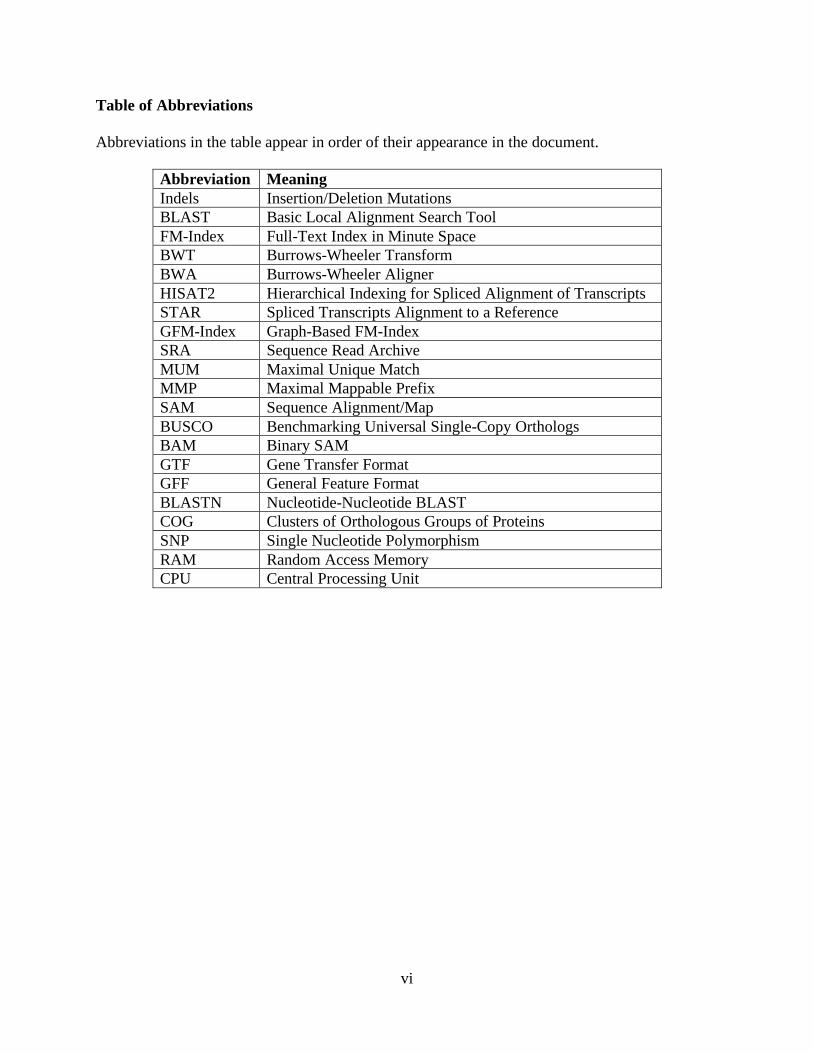
Table of Abbreviations

Abbreviations in the table appear in order of their appearance in the document.

Abbreviation Meaning

Indels Insertion/Deletion Mutations

BLAST Basic Local Alignment Search Tool

FM-Index Full-Text Index in Minute Space

BWT Burrows-Wheeler Transform

BWA Burrows-Wheeler Aligner

HISAT2 Hierarchical Indexing for Spliced Alignment of Transcripts

STAR Spliced Transcripts Alignment to a Reference

GFM-Index Graph-Based FM-Index

SRA Sequence Read Archive

MUM Maximal Unique Match

MMP Maximal Mappable Prefix

SAM Sequence Alignment/Map

BUSCO Benchmarking Universal Single-Copy Orthologs

BAM Binary SAM

GTF Gene Transfer Format

GFF General Feature Format

BLASTN Nucleotide-Nucleotide BLAST

COG Clusters of Orthologous Groups of Proteins

SNP Single Nucleotide Polymorphism

RAM Random Access Memory

CPU Central Processing Unit

1

Introduction

A large portion of biological research today involves the study of genetic mutations and

how these changes contribute to the overall chemical makeup of the organism. In its most

general form, genetic research comes down to a comparison between the DNA of multiple

organisms or subgroups and analyzing which mutations or gene variants are beneficial or

disadvantageous to those groups. On the simplest scale, one could study the differences between

a single gene that is common between two organisms. This can be done by aligning together the

sequences in a pairwise fashion and simply showing which bases are different. Most often

though a single gene comparison is not enough as many traits are considered polygenic and

would require the analysis and alignment of multiple genes. This leads to the larger scale studies

of comparing and aligning whole genomes, which can lead to the discovery of indels, gene

duplications, chromosomal inversions, etc. By comparing the genomes of plants of the same

species, one could identify which gene variants contribute to greater crop yield or increase

photosynthetic rates. The genomes of cancer cell lines can be analyzed to identify mutations

throughout multiple genes which are contributing to the accelerated growth of the cells. A newly

discovered pathogen’s genome could be examined for potential weaknesses to target, such as a

lack of antibiotic resistant genes, to protect the host. Through all these analyses, it is the aligning

of the genome itself that is often a crucial step in any genomics research as an inaccurate

alignment can lead to incorrect conclusions downstream. This step is further hampered by the

countless tools available for genome alignment claiming to be the best and most efficient at what

they do. In this project, the top genome alignment tools will be tested against one another to

determine the fastest and most accurate genome aligner.

2

After a genome is sequenced, the data obtained are many small reads each containing

about 100 base pairs or less. These reads represent the genome itself fragmented into small parts,

which essentially means that the current data is of limited utility for any analysis without

assembling a new genome or aligning to a reference. If a novel organism has been sequenced, a

genome assembler is used to stitch together the fragments based on overlapping segments in each

of the reads. This tends to be a time-consuming process as the genome is being created from

scratch and fragments may require additional rounds of sequencing to accurately fill in the

missing gaps. An aligner takes in a previously assembled reference genome and a set of

sequenced reads, often RNA sequencing data, and works to match the reads to their appropriate

position in the genome. With an already completed genome to work with, a genome aligner is

often preferred to save time. Although they seem to be less complex, there are often two major

problems that aligners must overcome: 1) accurately matching a read to its position in the

reference genome and 2) quickly processing large genome files.

Seed-and-Extend with Hash Tables

When it comes to matching a fragment to its position, the fragmented sequence will most

likely not be an exact match to the reference genome. This often is due to the frequency of

mutations in the DNA of the sequenced organism, errors during sequencing, or polymorphisms

that occur within a species. In 1990, the basic local alignment search tool (BLAST) was

published, which contained an algorithm used to align two sequences through a process called

seed-and-extend (Altschul et al., 1990). The algorithm starts by dividing the reference sequence

into fragments of a user-determined length k. These fragments are referred to as k-mers and the

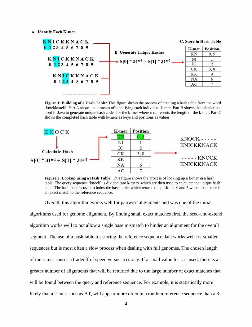
process of generating these fragments is shown in Figure 1-A. A k-mer is then run through an

equation to generate a unique numerical index, called a hash code. A simple example of this is

3

Java’s hash code calculation which adds the ASCII value of each character in the k-mer

multiplied by decreasing exponentials of base 31, shown in Figure 1-B. The generated hash code

is then used as an index to a structure called a hash table and used to store the position that the k-

mer occurs in the overall reference sequence as shown in Figure 1-C. Once the hash table is

created for the reference sequence, the query sequence is now split into k-mers of the same

length and inputted into the same hash code calculation to get an index. If the k-mer in the query

sequence is an exact match to a k-mer in the reference sequence, the hash table will return the

positions in the reference to begin the alignment as shown in Figure 2. The process of finding

exact matches between the query and reference sequence is known as seeding and makes up the

“seed” portion of the seed-and-extend algorithm. Once the algorithm finds the position of the

exact match, an attempt is made to extend the alignment before and after the position of the

match. During the extension stage, the algorithm uses a specific scoring system that gives

positive scores to exact base matches and negative scores to inexact matches. Once an alignment

falls below a specific scoring threshold, the alignment is returned to the user and either the next

position of an exact match is used for an alignment if available or the next k-mer from the query

sequence is used.

4

Figure 1: Building of a Hash Table: This figure shows the process of creating a hash table from the word

‘knickknack’. Part A shows the process of identifying each individual k-mer. Part B shows the calculation

used in Java to generate unique hash codes for the k-mer where n represents the length of the k-mer. Part C

shows the completed hash table with k-mers as keys and positions as values.

Figure 2: Lookup using a Hash Table: This figure shows the process of looking up a k-mer in a hash

table. The query sequence ‘knock’ is divided into k-mers, which are then used to calculate the unique hash

code. The hash code is used to index the hash table, which returns the positions 0 and 5 where the k-mer is

an exact match to the reference sequence.

Overall, this algorithm works well for pairwise alignments and was one of the initial

algorithms used for genome alignment. By finding small exact matches first, the seed-and-extend

algorithm works well to not allow a single base mismatch to hinder an alignment for the overall

segment. The use of a hash table for storing the reference sequence data works well for smaller

sequences but is most often a slow process when dealing with full genomes. The chosen length

of the k-mer causes a tradeoff of speed versus accuracy. If a small value for k is used, there is a

greater number of alignments that will be returned due to the large number of exact matches that

will be found between the query and reference sequence. For example, it is statistically more

likely that a 2-mer, such as AT, will appear more often in a random reference sequence than a 3-

5

mer, like ATG. However, the smaller k value causes a large amount of k-mer overlap which

results in many stored positions in the hash table. This slows down the algorithm as each position

requires an alignment to be created in the extension stage. In contrast, a large value for k will not

have as many positions stored and ultimately leads to a faster alignment that may not be as

accurate due to their needing to be an exact match between longer sequences in both the

reference and query.

Suffix Trees

To cut down on time taken for a genome alignment, an alignment tool called MUMmer

was released in 1999, which, among other updates, introduced the use of a suffix tree to replace

the hash table used in previous tools (Delcher et al., 1999). Suffix trees originated in the field of

computer science to search for substrings more efficiently within a large text file. MUMmer’s

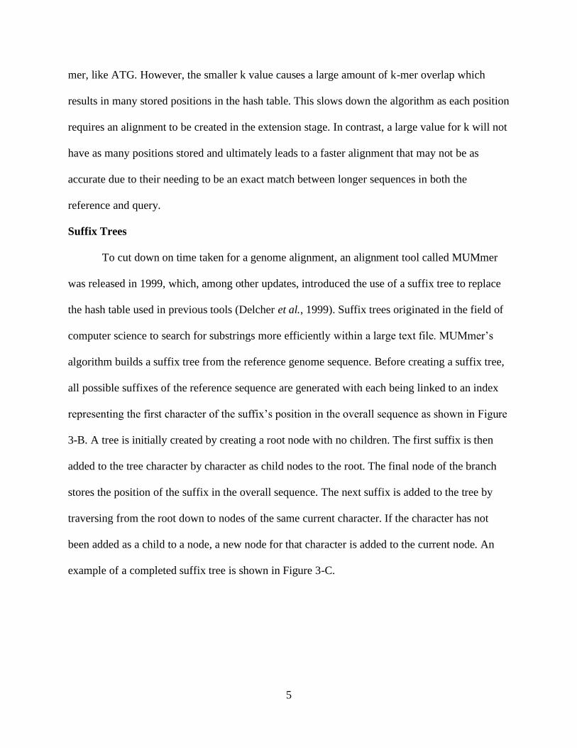
algorithm builds a suffix tree from the reference genome sequence. Before creating a suffix tree,

all possible suffixes of the reference sequence are generated with each being linked to an index

representing the first character of the suffix’s position in the overall sequence as shown in Figure

3-B. A tree is initially created by creating a root node with no children. The first suffix is then

added to the tree character by character as child nodes to the root. The final node of the branch

stores the position of the suffix in the overall sequence. The next suffix is added to the tree by

traversing from the root down to nodes of the same current character. If the character has not

been added as a child to a node, a new node for that character is added to the current node. An

example of a completed suffix tree is shown in Figure 3-C.

6

Figure 3: Creating a Suffix Tree: This figure shows the process of creating a suffix tree from the word

‘knickknack’. The overall word with its associated indexes is shown in part A. Part B shows all suffixes of

the word with their associated indexes. Part C shows the completed suffix tree.

Although building the suffix tree takes time for larger sequences, finding an exact match

to a k-mer of the sequenced reads is fast (linear-time) (Homer and Li, 2010). Lookup in a suffix

tree begins with finding k-mers of the query sequence and searching for exact matches in the

reference sequence by traversing down through the tree starting at the root as shown in Figure 4.

The traversed path is chosen by matching characters in the query k-mer to characters in a child

node. If a node with a position is met, then only one exact match exists at the indicated position

and extension of the alignment carries out as described previously. If traversal ends on an

internal node (such as shown in Figure 4), an alignment is automatically generated for each child

node off the current node. In this way, more than one alignment is created at the same time,

unlike the hash table method which requires each alignment to be processed separately.

Extension of the alignment is also made simpler by only having to traverse further down the tree

to align the next bases.

7

Figure 4: Lookup using a Suffix Tree: This figure shows how lookup works using a suffix tree of the

word ‘knickknack’. The query word ‘knock’ is divided into 2-mers which are then used to traverse through

the tree starting at the root. As a result of the lookup, there are two exact matches in the reference so there

are two alignments created.

A tradeoff to the increased speed of the suffix tree algorithm is its massive memory

requirement. A single character requires 1 byte of memory. This means that if an algorithm was

to store all 3 billion bases of the human genome in memory, then 3 billion bytes, or 3 gigabytes,

of memory space would be required. A suffix tree not only requires memory to store suffixes of

the whole reference genome, but also all data involving the structure of the tree. This includes

memory used for each individual node of the tree as well as all paths between nodes. This

amounts to requiring approximately 15 bytes per base, which would amount to 45 gigabytes of

memory to store a suffix tree for the human genome (Kurtz et al., 2004). This massive amount of

required memory makes computation impractical for large genomes and led researchers to look

elsewhere for more efficient algorithms.

FM-Index with BWT

The need to align larger genomes led to researchers adding a Full-text index in Minute

space (FM-Index) into a genome aligner algorithm (Ferragina and Manzini, 2000). An FM-Index

was regarded as the next evolution of a suffix tree for its low memory space and ability to be

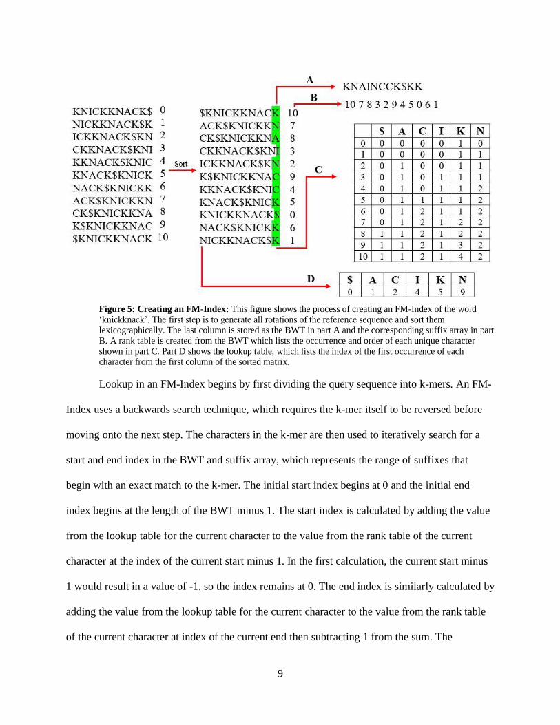
compressed even further. To create an FM-Index, an end of file character, typically $, is

8

appended to the reference string. This character is used later to identify where in the string the

end occurs. All rotations of the reference string are then generated in a matrix as shown in the

first step of Figure 5. A rotation of a string is simply the removal of the first character in the

string and appending it onto the end. A suffix array is also created for the matrix which stores the

index of the starting position of each suffix (all characters to the left of $) in the original string.

For example, the initial suffix starts at position 0, the first rotation starts at position 1, second

rotation at position 2, etc. The matrix is then sorted lexicographically by the first column, which

causes the suffix array to sort accordingly as well. The last column of the sorted matrix is

referred to as the Burrows-Wheeler transform (BWT) (shown as Figure 5-A) and is stored

alongside the sorted suffix array (shown as Figure 5-B). Using the BWT, a rank table is created

which contains a column for each unique symbol in the reference string and a row for each

character in the BWT. The table is filled starting at the 0th row and counts how many times and

in what order each symbol appears in the BWT. A completed example of a rank table is shown in

Figure 5-C. Based off the first column in the matrix, a lookup table is created that stores the

index/row of the first occurrence of each unique character. An example of this is shown in Figure

5-D, which shows the ‘$’ being in the 0th row of the sorted matrix, the first ‘A’ in row 1, the first

‘C’ in row 2, etc. Only the BWT, suffix array, rank table, and lookup table are stored in memory

and these four objects make up the completed FM-Index.

9

Figure 5: Creating an FM-Index: This figure shows the process of creating an FM-Index of the word

‘knickknack’. The first step is to generate all rotations of the reference sequence and sort them

lexicographically. The last column is stored as the BWT in part A and the corresponding suffix array in part

B. A rank table is created from the BWT which lists the occurrence and order of each unique character

shown in part C. Part D shows the lookup table, which lists the index of the first occurrence of each

character from the first column of the sorted matrix.

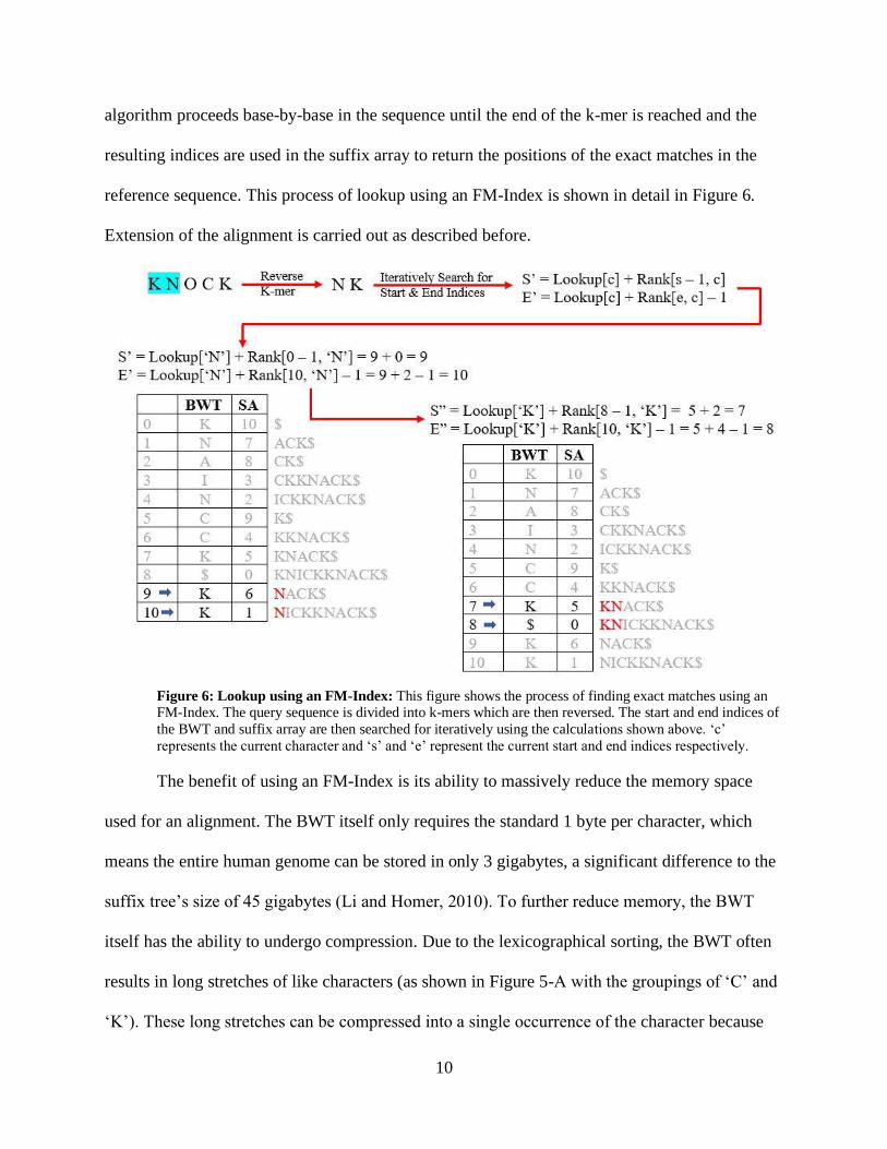
Lookup in an FM-Index begins by first dividing the query sequence into k-mers. An FM-

Index uses a backwards search technique, which requires the k-mer itself to be reversed before

moving onto the next step. The characters in the k-mer are then used to iteratively search for a

start and end index in the BWT and suffix array, which represents the range of suffixes that

begin with an exact match to the k-mer. The initial start index begins at 0 and the initial end

index begins at the length of the BWT minus 1. The start index is calculated by adding the value

from the lookup table for the current character to the value from the rank table of the current

character at the index of the current start minus 1. In the first calculation, the current start minus

1 would result in a value of -1, so the index remains at 0. The end index is similarly calculated by

adding the value from the lookup table for the current character to the value from the rank table

of the current character at index of the current end then subtracting 1 from the sum. The

10

algorithm proceeds base-by-base in the sequence until the end of the k-mer is reached and the

resulting indices are used in the suffix array to return the positions of the exact matches in the

reference sequence. This process of lookup using an FM-Index is shown in detail in Figure 6.

Extension of the alignment is carried out as described before.

Figure 6: Lookup using an FM-Index: This figure shows the process of finding exact matches using an FM-Index. The query sequence is divided into k-mers which are then reversed. The start and end indices of

the BWT and suffix array are then searched for iteratively using the calculations shown above. ‘c’

represents the current character and ‘s’ and ‘e’ represent the current start and end indices respectively.

The benefit of using an FM-Index is its ability to massively reduce the memory space

used for an alignment. The BWT itself only requires the standard 1 byte per character, which

means the entire human genome can be stored in only 3 gigabytes, a significant difference to the

suffix tree’s size of 45 gigabytes (Li and Homer, 2010). To further reduce memory, the BWT

itself has the ability to undergo compression. Due to the lexicographical sorting, the BWT often

results in long stretches of like characters (as shown in Figure 5-A with the groupings of ‘C’ and

‘K’). These long stretches can be compressed into a single occurrence of the character because

11

the length of the run can be inferred from a combination of the lookup and rank tables. In most

cases, memory is further reduced by not actually creating a suffix array to store alongside the

BWT. When the appropriate start and end index are found, the BWT, in column form, is reversed

back into the original reference sequence using repeated steps of prepending the BWT and

sorting the matrix lexicographically. In some algorithms using an FM-Index, the rank table only

stores data for every other row with missing data being inferred from the surrounding data. The

low memory space for using an FM-Index allows for the alignment of large genomes to be

computationally practical.

Modern Aligners

The aligners being used in this project are Bowtie2, Burrows-Wheeler Aligner (BWA),

Hierarchical Indexing for Spliced Alignment of Transcripts (HISAT2), MUMmer4, Spliced

Transcripts Alignment to a Reference (STAR), and TopHat2.

Bowtie2

The first iteration of Bowtie was released in 2008 and performed ungapped alignments of

short reads (approximately 35 base pairs) (Langmead et al., 2009). The assumption behind not

allowing gaps in the alignments was that shorter reads should have a unique place in the genome

and not accounting for gaps allows the aligner to run much faster. With longer reads, this

assumption results in low alignment rates and does not allow for the alignment of RNA

sequences to a genome (as any introns in the gene will automatically add gaps to the RNA

alignment). In addition to ungapped alignments, Bowtie only performed alignments in end-to-

end mode. This method of alignment requires that an entire read be aligned from one end to the

other in order for the alignment to be reported to the user. This often leads to lower alignment

scores and forced alignments if the ends of reads are not trimmed properly for quality control. In

12

2011, Bowtie2 was released which built upon the previous ungapped alignments of Bowtie by

accounting for the addition of gaps (Langmead and Salzberg, 2012). Bowtie2 uses an FM-Index

to index the genome and seeds a query sequence to find multiple ungapped alignments which are

then extended, which is similar to Bowtie. An extra step for Bowtie2 allows for multiple “seeds”

to be combined together based on their proximity to each other, which accounts for adding gaps

to create larger alignments. Bowtie2 also is able to run in both end-to-end and local mode for

generating alignments. In local mode, the aligner is able to trim bases from either end of the read

to increase alignment scores and not be hindered by low-quality bases on the end of reads

leftover from poor quality control. Regardless of the mode being run, Bowtie2 generates multiple

alignments for each read but only reports the single best alignment per read. A downside to

Bowtie2 is that the aligner was designed with the intent of aligning DNA reads to a reference

genome and does not allow for the addition of a transcript annotation file to aid in the mapping

of RNA reads.

BWA

The BWA tool initially released in 2008 as an aligner for mapping short reads under 100

base pairs long. To index the genome, BWA uses a combination of the Burrows-Wheeler

transform and an FM-Index to achieve a linear lookup time for finding exact matches to a given

k-mer (a sequence of length n is found in O(n) time) (Li and Durbin, 2009). This method of

indexing the genome has remained virtually unchanged through the years, however, the

alignment algorithm itself has been updated to accommodate longer reads. The BWA-MEM

algorithm, released in 2012, is designed to be used for reads of all sizes (Li, 2013). The aligner

works by first seeding a query sequence by searching for exact matches in the reference genome

using a k-mer size of 19 by default. BWA-MEM then extends a seed until a given cutoff value is

13

reached, which is calculated by a function which does not penalize large gaps in the resulting

alignment. Unlike Bowtie2 (which allows the user to choose one mode or the other), BWA-

MEM’s extension algorithm stores the best alignment score for both an end-to-end (if the end of

the query is reached during extension) and local alignment and reports the better alignment (with

a bias toward choosing end-to-end alignments for longer alignments). By storing multiple

alignments, BWA-MEM also has the ability to report multiple alignments per read in the form of

secondary and supplementary alignments (on by default). Like Bowtie2, a downside to the

BWA-MEM algorithm is that it was originally created to align DNA reads to a reference genome

and therefore does not have the ability to import a transcript file to identify splice junctions in

RNA.

HISAT2

HISAT was released in 2014 with the intent to align RNA-seq reads and was created by

the same developers of both TopHat and Bowtie (Kim, Langmead, and Salzberg, 2015). HISAT

indexes the genome using a method similar to Bowtie’s FM-Index. A major difference between

these aligners is that HISAT uses one large FM-Index, which covers the entire genome, and

many smaller FM-Indexes, where each smaller index accounts for 64,000 base pair portions of

the genome with about 1,000 base pairs of overlap between consecutive areas. Not long after the

release of HISAT, HISAT2 was created in 2015 which implemented a graph-based FM-Index

(GFM) to index the reference genome, the first time an algorithm of this kind was ever

developed (Kim et al., 2019). The GFM-Index used by HISAT2 works similarly to HISAT’s one

larger and multiple smaller indexes, however, using a graph-based approach allows the aligner to

take in SRA data to add variants into the index which could occur in the form of insertions,

deletions, or mutations. The GFM-Index allows for multiple paths to be created through the

14

genome index with one path being the original reference sequence and other paths in the index

representing a different variant. This type of approach works well for most model organisms

where variant data is known. If SRA data is not added as input, HISAT2 defaults to creating the

FM-Index created by HISAT. HISAT2 also deals with repetitive sequences differently than other

aligners by combining repeat sequences in the reference genome into one sequence. This reduces

the number of alignments reported by only reporting one alignment for a read aligning to these

regions rather than one per repetitive element. As HISAT2 is designed to align both genomic and

RNA reads, the ability to input a file of known splice sites allows for better mapping of exons to

places in the genome.

MUMmer4

One of the oldest aligners, MUMmer, was released in 1999 with the goal of aligning

whole genomes to one another (Delcher et al., 1999). MUMmer’s initial form of genome

indexing was the use of a suffix tree alongside the assumption that the genomes are from closely

related organisms. Using this assumption, MUMmer then looks for maximal unique matches

(MUMs) between the genomes, which is the largest possible subsequence of 100% identity that

occurs once in each genome. The alignment is then built from the MUMs that are found. As

suffix trees require large amounts of memory in order to be built, MUMmer was redefined over

the years to reduce memory space and increase speed with the release of MUMmer2 and

MUMmer3 (Delcher et al., 2002; Kurtz et al., 2004). MUMmer3, in particular, added the ability

to align non-unique MUMs which are large subsequences that can occur multiple times in the

reference but still only once in the query. To further reduce memory space, the release of

MUMmer4 replaced the suffix tree index with a suffix array, which allows for the processing of

genomes up to 141 trillion base pairs (larger than any known genome by 1000x) (Marçais et al.,

15

2018). To increase runtime, MUMmer4 allowed for the use of multiple cores to process

alignments across more than one computing core and the ability to pre-build the reference

genome index to then be loaded in later for alignments to the same reference.

STAR

Built primarily to handle mapping of RNA-seq data, STAR was released in 2012 with the

intent on tackling the issue of mapping spliced RNA transcripts (Dobin et al., 2013). STAR

indexes the reference genome using an uncompressed version of a suffix array, which often takes

up a large amount of memory (due to it being uncompressed) and time in order to build. This

type of data structure (as is used by MUMmer4 as well) has a fast searching time and can handle

nearly any size genome. To cut down on the runtime for successive alignments, STAR allows for

the genome to be pre-built once and the resulting indexes to be loaded in for each individual

alignment, which drastically decreases the runtime. To identify matches between reference and

query, STAR uses a similar approach to MUMmer’s maximal unique match approach, but adapts

this methodology to spliced RNA. As most RNA transcripts will be made up of multiple exons,

one alignment is often not enough for a given transcript as the first half the read may map to

location A and the second half to location B with a large intron inbetween the two. To

accommodate this, STAR identifies a Maximal Mappable Prefix (MMP), which is simply the

longest exact match to the genome starting from the first base of a query read. This results in the

first half of the read given a seeded location in the reference genome which is then extended to

generate the alignment. This step is then repeated for the next portion of the query sequence that

did not belong to the first alignment. This allows for a single RNA transcript to be aligned to

multiple locations in the genome and accounting for splice junctions within the read. Further

16

adding to its ability to correctly align spliced transcripts, STAR provides the option of inputting

an annotation file of known splice junctions to aid in the process of identifying MMPs.

TopHat2

Building upon the success of Bowtie, TopHat was created in 2009 as a tool to refine

Bowtie’s alignment of DNA to aligning RNA across splice junctions (Trapnell, Pachter, and

Salzberg, 2009). The first iteration of TopHat worked by performing an initial alignment of all

reads with Bowtie (using end-to-end mode). Those reads that mapped well from end-to-end were

passed through as alignments without splice junctions. An alignment with a splice junction

would report relatively low scores due to the large gaps and/or mismatches identified using end-

to-end mode. Those reads which were not mapped are then sent through a second round of

alignment using a simple seed-and-extend algorithm to identify potential splice junctions that

would not have been reported during an end-to-end alignment. The release of TopHat2 in 2012

would incorporate the use of Bowtie2 into the first stage of alignment (Kim et al., 2013). In

addition, TopHat2 allowed for the input of a file containing known splice junctions to aid in

alignment as well as the ability to directly align reads to an inputted transcriptome rather than an

entire reference genome. As TopHat2 uses Bowtie2 under the hood, all of Bowtie2’s default

parameters are used including the indexing of the genome using an FM-Index. Recently,

TopHat2 has been overshadowed by the release of HISAT2, which were created by the same

developers.

Project Goal

As genome aligners have evolved over time, the underlying algorithms that are built-in

have evolved with them. Although changes are made to fix certain facets of the aligner, the

updated algorithms often must sacrifice speed for accuracy or vice versa. The goal of this project

17

is to determine which aligner achieves the best balance between runtime and accuracy and

ultimately determine the best aligner. This will be done by running each aligner in a controlled

enviroment using default settings and the same data sets.

Materials & Methods

Sequence Generation

The query samples used for this project were 48 samples of Erysiphe necator, more

commonly known as the fungal disease powdery mildew, and were obtained from the lab of Dr.

Lance Cadle-Davidson of the United States Department of Agriculture. Samples were grown on

the leaves of Vitis vinifera in diverse geographical regions (see Supplementary S4). RNA was

isolated from the fungal samples by using clear nail polish on the infected leaves to separate the

fungal tissue from the leaves followed by RNA extraction (Cadle-Davidson et al., 2009).

Samples were sequenced in one single-end run of an Illumina GA HiSeq with 5 base-pair

barcodes provided for each isolate. The pooled library of reads was run through the barcode

splitter of the FASTX-toolkit (v0.0.13) (Hannon, 2010) to create a separate file of reads for each

of the 48 isolates. The reference genome scaffold for Erysiphe necator (C-strain) used in this

project was obtained from the Cantu Lab at UC Davis (https://cantulab.github.io/e-

necator.scaffolds.c.NCBI.fasta.gz; Jones et al, 2014).

Quality Control

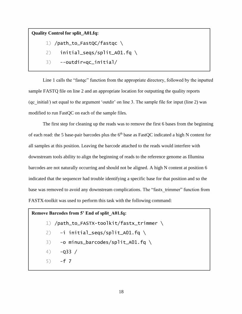
Raw reads were checked for their initial quality using FastQC (v0.11.7) (Andrews, 2018).

Initial quality of any sequencing reads should always be checked to determine if there is a need

for any base trimming, sequencing adapters to remove, etc. The following command was used to

check quality of the reads using FastQC:

18

Line 1 calls the “fastqc” function from the appropriate directory, followed by the inputted

sample FASTQ file on line 2 and an appropriate location for outputting the quality reports

(qc_initial/) set equal to the argument ‘outdir’ on line 3. The sample file for input (line 2) was

modified to run FastQC on each of the sample files.

The first step for cleaning up the reads was to remove the first 6 bases from the beginning

of each read: the 5 base-pair barcodes plus the 6th base as FastQC indicated a high N content for

all samples at this position. Leaving the barcode attached to the reads would interfere with

downstream tools ability to align the beginning of reads to the reference genome as Illumina

barcodes are not naturally occurring and should not be aligned. A high N content at position 6

indicated that the sequencer had trouble identifying a specific base for that position and so the

base was removed to avoid any downstream complications. The “fastx_trimmer” function from

FASTX-toolkit was used to perform this task with the following command:

Quality Control for split_A01.fq:

1) /path_to_FastQC/fastqc \

2) initial_seqs/split_A01.fq \

3) --outdir=qc_initial/

Remove Barcodes from 5’ End of split_A01.fq:

1) /path_to_FASTX-toolkit/fastx_trimmer \

2) –i initial_seqs/split_A01.fq \

3) -o minus_barcodes/split_A01.fq \

4) -Q33 /

5) -f 7

19

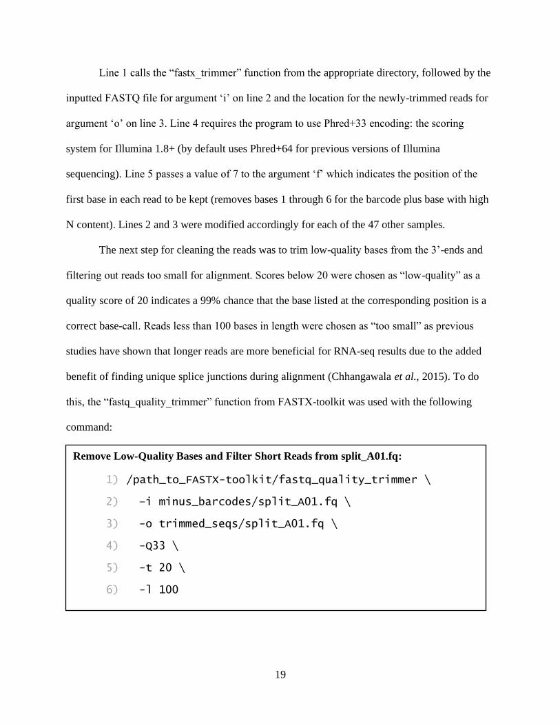
Line 1 calls the “fastx_trimmer” function from the appropriate directory, followed by the

inputted FASTQ file for argument ‘i’ on line 2 and the location for the newly-trimmed reads for

argument ‘o’ on line 3. Line 4 requires the program to use Phred+33 encoding: the scoring

system for Illumina 1.8+ (by default uses Phred+64 for previous versions of Illumina

sequencing). Line 5 passes a value of 7 to the argument ‘f’ which indicates the position of the

first base in each read to be kept (removes bases 1 through 6 for the barcode plus base with high

N content). Lines 2 and 3 were modified accordingly for each of the 47 other samples.

The next step for cleaning the reads was to trim low-quality bases from the 3’-ends and

filtering out reads too small for alignment. Scores below 20 were chosen as “low-quality” as a

quality score of 20 indicates a 99% chance that the base listed at the corresponding position is a

correct base-call. Reads less than 100 bases in length were chosen as “too small” as previous

studies have shown that longer reads are more beneficial for RNA-seq results due to the added

benefit of finding unique splice junctions during alignment (Chhangawala et al., 2015). To do

this, the “fastq_quality_trimmer” function from FASTX-toolkit was used with the following

command:

Remove Low-Quality Bases and Filter Short Reads from split_A01.fq:

1) /path_to_FASTX-toolkit/fastq_quality_trimmer \

2) –i minus_barcodes/split_A01.fq \

3) -o trimmed_seqs/split_A01.fq \

4) -Q33 \

5) -t 20 \

6) -l 100

20

Line 1 calls the “fastq_quality_trimmer” function from the appropriate directory,

followed by the inputted FASTQ file (output from “fastx_trimmer”) for argument ‘i’ on line 2

and the location for the outputted trimmed reads for argument ‘o’ on line 3. Line 4 requires the

program to use Phred+33 encoding as previously described for “fastx_trimmer”. Line 5 shows

the cutoff value for low quality bases (bases with scores under 20 removed) to be trimmed from

the 3’ end of each read and line 6 corresponds to the minimum length for each read (reads under

100 bases after trimming are removed). Lines 2 and 3 were modified accordingly for each of the

47 other samples.

To check the quality post-filtering, the trimmed sample files were used as input into

FastQC once more. The output of FastQC indicated sufficient filtering was performed and all

samples were ready for use in the subsequent methods. The number of reads pre- and post-

trimming were recorded to calculate the percentage of reads leftover from filtering.

Alignment Generation

For all aligners, the first step was to index the reference genome. This step is not required

for a run of the aligner, however, building the genome index prior to alignment allows the aligner

to call the index for each run. This means that the genome index will not have to be created for

individual run. This helps to reduce the runtime of individual runs of the aligner and removes

any variability regarding different indexing techniques impacting the timing statistics for each

sample. Creating the reference genome index is the only pre-processing step performed to run

each of the aligners. After creating the genome index, the aligners can be run on each sample

individually by reading in the sample file and the pre-built genome index. All aligners were run

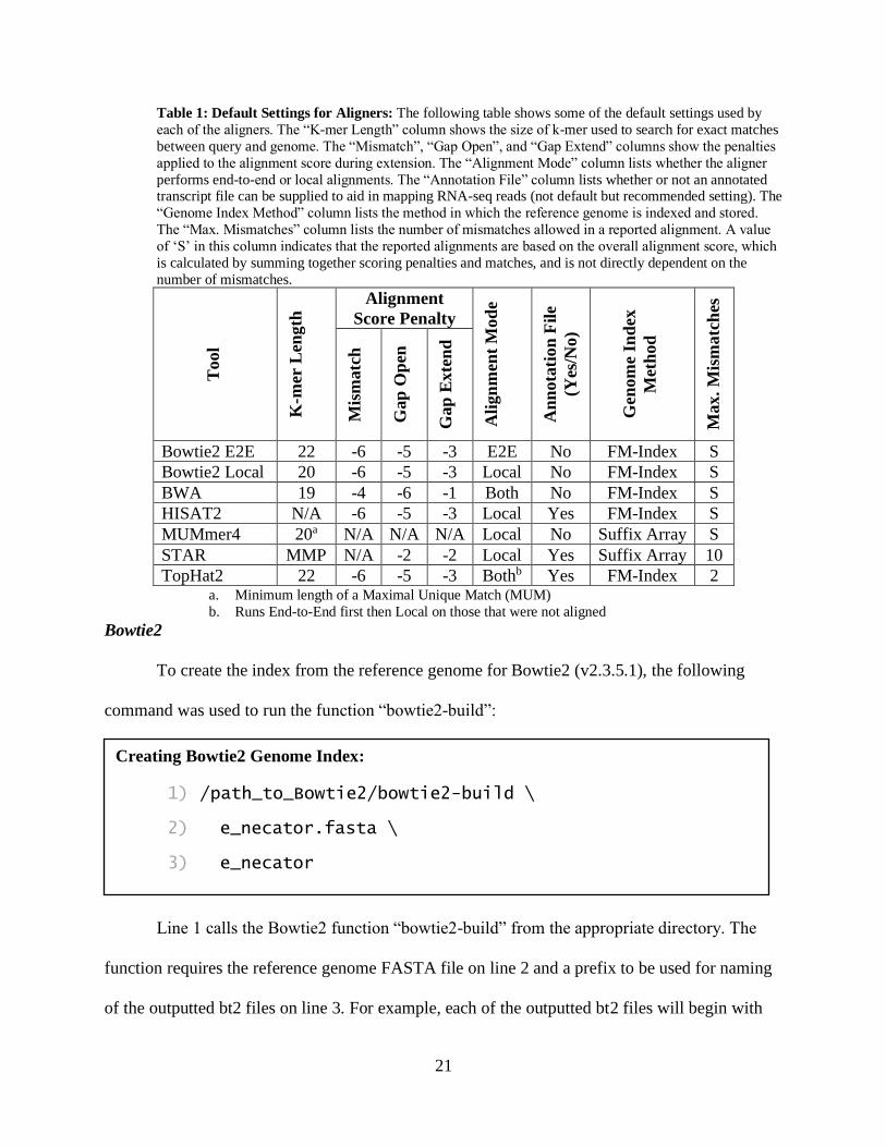
using the default parameters with some of these values outlined in Table 1.

21

Table 1: Default Settings for Aligners: The following table shows some of the default settings used by

each of the aligners. The “K-mer Length” column shows the size of k-mer used to search for exact matches

between query and genome. The “Mismatch”, “Gap Open”, and “Gap Extend” columns show the penalties

applied to the alignment score during extension. The “Alignment Mode” column lists whether the aligner

performs end-to-end or local alignments. The “Annotation File” column lists whether or not an annotated transcript file can be supplied to aid in mapping RNA-seq reads (not default but recommended setting). The

“Genome Index Method” column lists the method in which the reference genome is indexed and stored.

The “Max. Mismatches” column lists the number of mismatches allowed in a reported alignment. A value

of ‘S’ in this column indicates that the reported alignments are based on the overall alignment score, which

is calculated by summing together scoring penalties and matches, and is not directly dependent on the

number of mismatches.

Tool

K-m

er L

ength

Alignment

Score Penalty

Ali

gn

men

t M

od

e

An

nota

tion

Fil

e

(Yes

/No)

Gen

om

e In

dex

Met

hod

Max.

Mis

matc

hes

Mis

matc

h

Ga

p O

pen

Gap

Exte

nd

Bowtie2 E2E 22 -6 -5 -3 E2E No FM-Index S

Bowtie2 Local 20 -6 -5 -3 Local No FM-Index S

BWA 19 -4 -6 -1 Both No FM-Index S

HISAT2 N/A -6 -5 -3 Local Yes FM-Index S

MUMmer4 20a N/A N/A N/A Local No Suffix Array S

STAR MMP N/A -2 -2 Local Yes Suffix Array 10

TopHat2 22 -6 -5 -3 Bothb Yes FM-Index 2 a. Minimum length of a Maximal Unique Match (MUM) b. Runs End-to-End first then Local on those that were not aligned

Bowtie2

To create the index from the reference genome for Bowtie2 (v2.3.5.1), the following

command was used to run the function “bowtie2-build”:

Line 1 calls the Bowtie2 function “bowtie2-build” from the appropriate directory. The

function requires the reference genome FASTA file on line 2 and a prefix to be used for naming

of the outputted bt2 files on line 3. For example, each of the outputted bt2 files will begin with

Creating Bowtie2 Genome Index:

1) /path_to_Bowtie2/bowtie2-build \

2) e_necator.fasta \

3) e_necator

22

“e_necator” such as “e_necator.1.bt2”, “e_necator.2.bt2”, etc. This command only needs to be

run once as all samples use the same reference genome.

Bowtie2 has two different modes for alignment: End-to-End and Local. When run in

End-to-End (default) mode, all characters from a given read are required to be aligned in the

reference genome. This requires reads to be fairly cleaned of any adapter sequences or

troublesome bases near the 3’-end as these bases will negatively impact the alignment of the

read. In Local mode, bases from a given read can be trimmed from either the 5’- or 3’-end if the

removal of these bases results in an increase in alignment scores for the read.

To run Bowtie2 in End-to-End mode, the following command was run:

Line 1 calls the Bowtie2 function “bowtie2” which runs the Bowtie2 alignment

algorithm. To read in the indexed reference genome, the prefix used for the outputted bt2 files of

the “bowtie2-build” function (“e_necator”) is used as input for argument ‘o’ as shown on line 2.

Line 3 shows the path for the outputted file (“A01.sam”) used for argument ‘S’ which indicates

that the outputted alignment file should be in SAM format. To the run the alignment with 5 cores

in parallel, 5 was used as input for the ‘p’ argument which indicates the number of cores to be

used for parallel computing. Line 6 indicates that the aligner should be run in End-to-End mode.

Run Bowtie2 on split_A01.fq in End-to-End Mode:

1) /path_to_Bowtie2/bowtie2 \

2) -x e_necator \

3) trimmed_seqs/split_A01.fq \

4) -S /path_to_output/A01.sam \

5) -p 5 \

6) --end-to-end

23

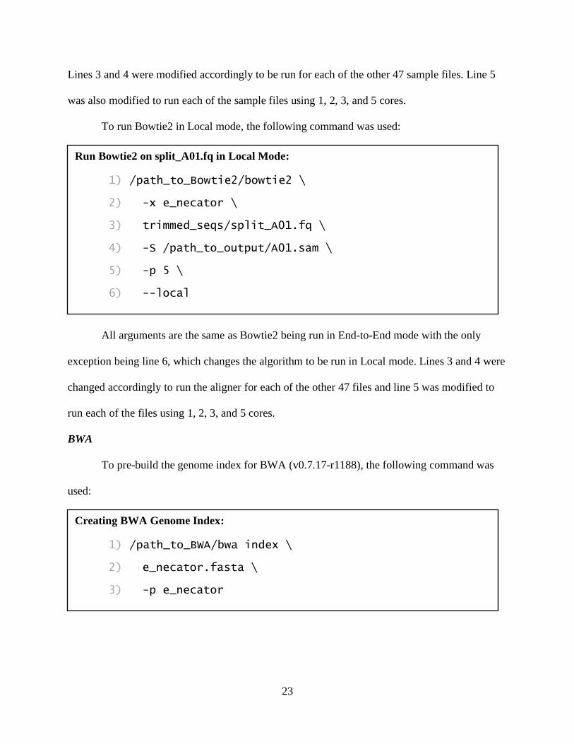
Lines 3 and 4 were modified accordingly to be run for each of the other 47 sample files. Line 5

was also modified to run each of the sample files using 1, 2, 3, and 5 cores.

To run Bowtie2 in Local mode, the following command was used:

All arguments are the same as Bowtie2 being run in End-to-End mode with the only

exception being line 6, which changes the algorithm to be run in Local mode. Lines 3 and 4 were

changed accordingly to run the aligner for each of the other 47 files and line 5 was modified to

run each of the files using 1, 2, 3, and 5 cores.

BWA

To pre-build the genome index for BWA (v0.7.17-r1188), the following command was

used:

Run Bowtie2 on split_A01.fq in Local Mode:

1) /path_to_Bowtie2/bowtie2 \

2) -x e_necator \

3) trimmed_seqs/split_A01.fq \

4) -S /path_to_output/A01.sam \

5) -p 5 \

6) --local

Creating BWA Genome Index:

1) /path_to_BWA/bwa index \

2) e_necator.fasta \

3) -p e_necator

24

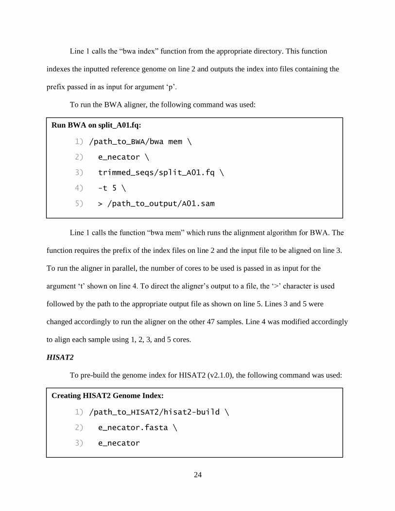
Line 1 calls the “bwa index” function from the appropriate directory. This function

indexes the inputted reference genome on line 2 and outputs the index into files containing the

prefix passed in as input for argument ‘p’.

To run the BWA aligner, the following command was used:

Line 1 calls the function “bwa mem” which runs the alignment algorithm for BWA. The

function requires the prefix of the index files on line 2 and the input file to be aligned on line 3.

To run the aligner in parallel, the number of cores to be used is passed in as input for the

argument ‘t’ shown on line 4. To direct the aligner’s output to a file, the ‘>’ character is used

followed by the path to the appropriate output file as shown on line 5. Lines 3 and 5 were

changed accordingly to run the aligner on the other 47 samples. Line 4 was modified accordingly

to align each sample using 1, 2, 3, and 5 cores.

HISAT2

To pre-build the genome index for HISAT2 (v2.1.0), the following command was used:

Run BWA on split_A01.fq:

1) /path_to_BWA/bwa mem \

2) e_necator \

3) trimmed_seqs/split_A01.fq \

4) -t 5 \

5) > /path_to_output/A01.sam

Creating HISAT2 Genome Index:

1) /path_to_HISAT2/hisat2-build \

2) e_necator.fasta \

3) e_necator

25

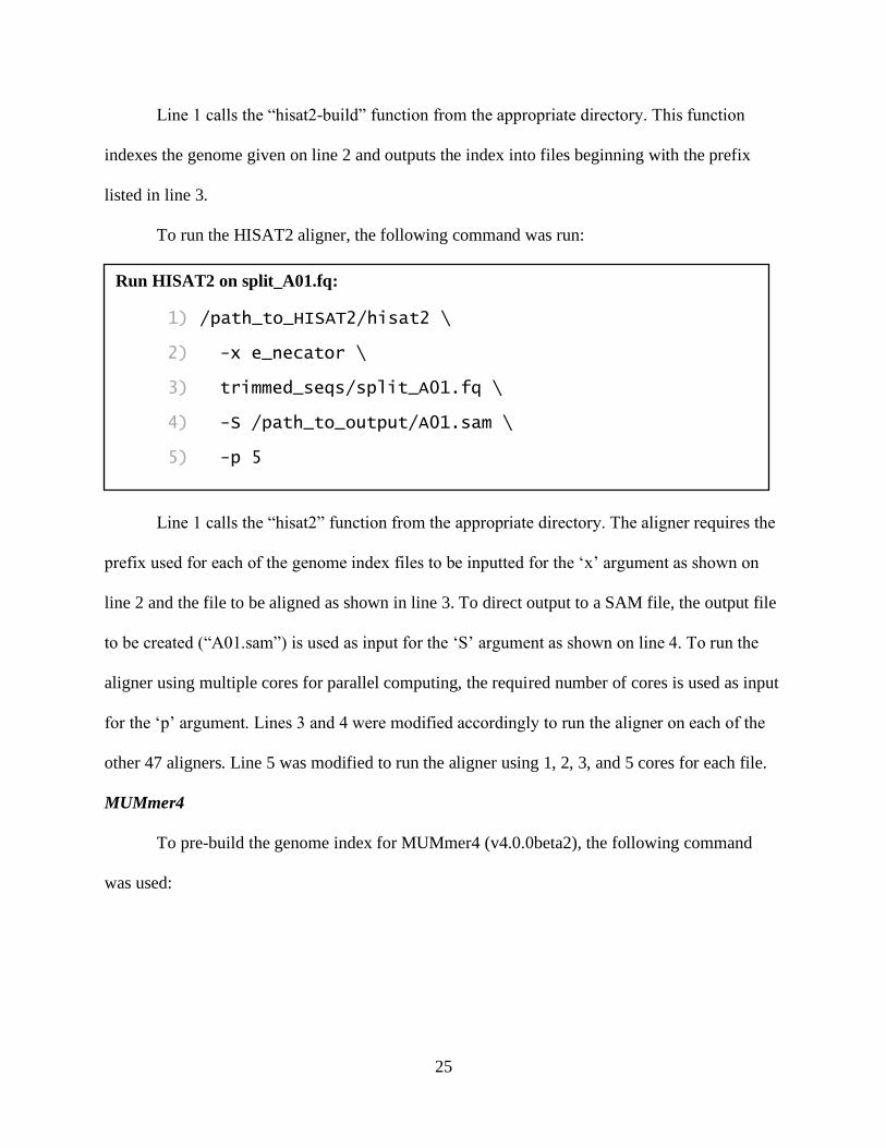
Line 1 calls the “hisat2-build” function from the appropriate directory. This function

indexes the genome given on line 2 and outputs the index into files beginning with the prefix

listed in line 3.

To run the HISAT2 aligner, the following command was run:

Line 1 calls the “hisat2” function from the appropriate directory. The aligner requires the

prefix used for each of the genome index files to be inputted for the ‘x’ argument as shown on

line 2 and the file to be aligned as shown in line 3. To direct output to a SAM file, the output file

to be created (“A01.sam”) is used as input for the ‘S’ argument as shown on line 4. To run the

aligner using multiple cores for parallel computing, the required number of cores is used as input

for the ‘p’ argument. Lines 3 and 4 were modified accordingly to run the aligner on each of the

other 47 aligners. Line 5 was modified to run the aligner using 1, 2, 3, and 5 cores for each file.

MUMmer4

To pre-build the genome index for MUMmer4 (v4.0.0beta2), the following command

was used:

Run HISAT2 on split_A01.fq:

1) /path_to_HISAT2/hisat2 \

2) -x e_necator \

3) trimmed_seqs/split_A01.fq \

4) -S /path_to_output/A01.sam \

5) -p 5

26

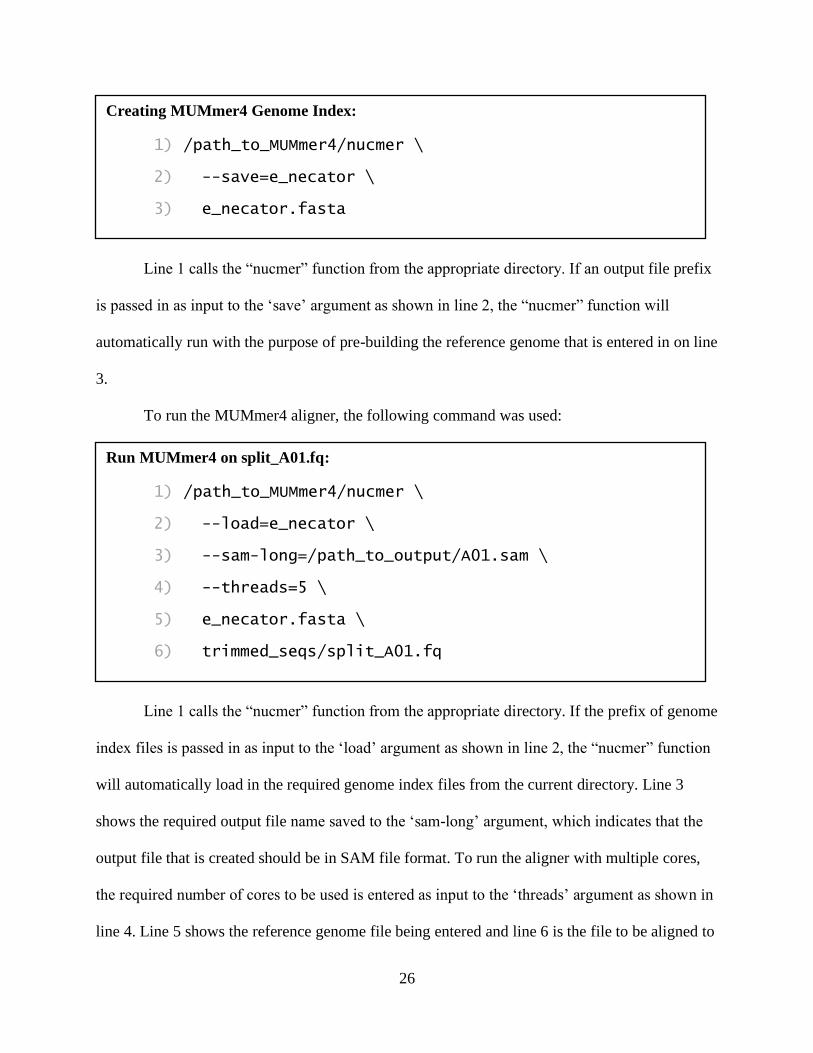
Line 1 calls the “nucmer” function from the appropriate directory. If an output file prefix

is passed in as input to the ‘save’ argument as shown in line 2, the “nucmer” function will

automatically run with the purpose of pre-building the reference genome that is entered in on line

3.

To run the MUMmer4 aligner, the following command was used:

Line 1 calls the “nucmer” function from the appropriate directory. If the prefix of genome

index files is passed in as input to the ‘load’ argument as shown in line 2, the “nucmer” function

will automatically load in the required genome index files from the current directory. Line 3

shows the required output file name saved to the ‘sam-long’ argument, which indicates that the

output file that is created should be in SAM file format. To run the aligner with multiple cores,

the required number of cores to be used is entered as input to the ‘threads’ argument as shown in

line 4. Line 5 shows the reference genome file being entered and line 6 is the file to be aligned to

Creating MUMmer4 Genome Index:

1) /path_to_MUMmer4/nucmer \

2) --save=e_necator \

3) e_necator.fasta

Run MUMmer4 on split_A01.fq:

1) /path_to_MUMmer4/nucmer \

2) --load=e_necator \

3) --sam-long=/path_to_output/A01.sam \

4) --threads=5 \

5) e_necator.fasta \

6) trimmed_seqs/split_A01.fq

27

the reference. Lines 3 and 6 were modified accordingly to run the aligner on each of the 47 other

files. Line 4 was modified to run each of the files using 1, 2, 3, and 5 cores.

After running the alignments, it was discovered that MUMmer4 does not create the

correct header for its SAM file alignment. This results in the outputted alignment file being

unable to be used as input for downstream analysis. Through further analysis of the SAM file

headers, each outputted file was missing the ‘@SQ’ header lines. These lines appear one for each

contig in the reference genome and list the name of the contig followed by the length of the

contig all in the same line. As these lines refer to the reference genome and do not depend on an

individual aligner, the ‘@SQ’ are identical between all outputted alignment files regardless of

the aligner. For this reason, lines taken from the MUMmer4 SAM files were combined with the

‘@SQ’ header lines from a correct SAM header from another aligner (the alignment of A01

using BWA) using a series of “grep” (v2.27) commands to correctly assemble a SAM file header

usable by downstream tools (see Supplementary B12).

STAR

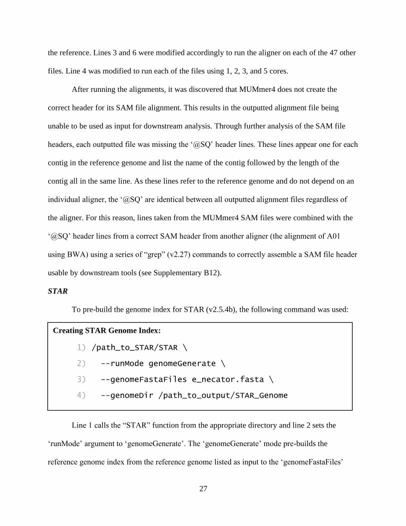
To pre-build the genome index for STAR (v2.5.4b), the following command was used:

Line 1 calls the “STAR” function from the appropriate directory and line 2 sets the

‘runMode’ argument to ‘genomeGenerate’. The ‘genomeGenerate’ mode pre-builds the

reference genome index from the reference genome listed as input to the ‘genomeFastaFiles’

Creating STAR Genome Index:

1) /path_to_STAR/STAR \

2) --runMode genomeGenerate \

3) --genomeFastaFiles e_necator.fasta \

4) --genomeDir /path_to_output/STAR_Genome

28

argument in line 3 and stores the resulting index files in the directory “STAR_Genome”, which

is listed as input to the ‘genomeDir’ argument as shown in line 4.

To run the STAR aligner, the following command was used:

Line 1 calls the “STAR” function from the appropriate directory, which by default uses

the ‘alignReads’ mode for the ‘runMode’ parameter so there is no need to update this argument.

The aligner takes in the path to the directory where the pre-built reference genome was stored as

input to the ‘genomeDir’ argument as shown in line 2. The file to be aligned is entered as input

to the ‘readFilesIn’ argument as shown in line 3 and the prefix and output path for the outputted

alignment files is used as input to the ‘outFileNamePrefix’ argument as shown in line 4. To run

the aligner using multiple cores, the required number of cores to be used is entered as input to the

‘runThreadN’ argument as shown in line 5. Lines 3 and 4 were changed accordingly to run the

aligner on each of the 47 other files. Line 5 was modified accordingly to run the aligner on each

file using 1, 2, 3, and 5 cores.

TopHat2

Since TopHat2 uses Bowtie2, the commands used to pre-build the genome index for

Bowtie2 were the same used for TopHat2 (see Bowtie2 section for the exact command). To run

the TopHat2 aligner, the following command was used:

Run STAR on split_A01.fq:

1) /path_to_STAR/STAR \

2) --genomeDir /path_to_index/STAR_Genome \

3) --readFilesIn trimmed_seqs/split_A01.fq \

4) --outFileNamePrefix /path_to_output/A01_ \

5) --runThreadN 5

29

Line 1 calls the “tophat” function from the appropriate directory. TopHat2 creates a

directory with outputted alignment files and the name/path to this directory can be added as input

to the ‘o’ argument as shown in line 2. The prefix used for the pre-built reference genome index

files is entered as input in line 3 followed by the file to be aligned in line 4. To run the aligner

using multiple cores, the number of cores to be used is added as input to the ‘p’ argument in as

shown in line 5. Lines 2 and 4 were modified accordingly to run the aligner on each of the 47

other files. Line 5 was change accordingly to run each of the files using 1, 2, 3, and 5 cores.

Alignment Assessment

To assess how well an aligner performed, three major variables were tracked: runtime

required, percentage of reads that were mapped to the reference genome (called alignment rate),

and total coverage of the transcriptome.

Time

To track the runtime of each aligner, the “time” function was used to track the runtime in

seconds for each file’s alignment. Runtime was recorded for an aligner during both pre-

processing and for each individual sample being aligned. Overall, there were four times recorded

for each file run: time for the aligner run using 1 core, 2 cores, 3 cores, and 5 cores. Each

samples runtime was normalized by the number of reads by dividing the time taken on X number

Run TopHat2 on split_A01.fq:

1) /path_to_TopHat2/tophat \

2) -o /path_to_output/A01 \

3) e_necator \

4) trimmed_seqs/split_A01.fq \

5) -p 5

30

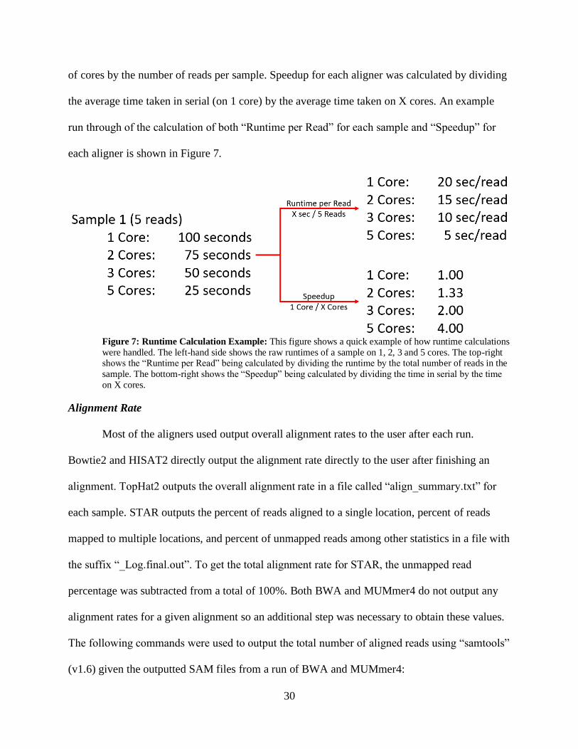
of cores by the number of reads per sample. Speedup for each aligner was calculated by dividing

the average time taken in serial (on 1 core) by the average time taken on X cores. An example

run through of the calculation of both “Runtime per Read” for each sample and “Speedup” for

each aligner is shown in Figure 7.

Figure 7: Runtime Calculation Example: This figure shows a quick example of how runtime calculations

were handled. The left-hand side shows the raw runtimes of a sample on 1, 2, 3 and 5 cores. The top-right shows the “Runtime per Read” being calculated by dividing the runtime by the total number of reads in the

sample. The bottom-right shows the “Speedup” being calculated by dividing the time in serial by the time

on X cores.

Alignment Rate

Most of the aligners used output overall alignment rates to the user after each run.

Bowtie2 and HISAT2 directly output the alignment rate directly to the user after finishing an

alignment. TopHat2 outputs the overall alignment rate in a file called “align_summary.txt” for

each sample. STAR outputs the percent of reads aligned to a single location, percent of reads

mapped to multiple locations, and percent of unmapped reads among other statistics in a file with

the suffix “_Log.final.out”. To get the total alignment rate for STAR, the unmapped read

percentage was subtracted from a total of 100%. Both BWA and MUMmer4 do not output any

alignment rates for a given alignment so an additional step was necessary to obtain these values.

The following commands were used to output the total number of aligned reads using “samtools”

(v1.6) given the outputted SAM files from a run of BWA and MUMmer4:

31

Line 1 calls the “samtools” function “view” rate is to convert the SAM file to a BAM file

using the “view” function of “samtools” as shown in line 1. Each read in a SAM file has a

distinct flag which marks it as one of a variety of alignments. The three relevant types to be

excluded for counting were unmapped reads, secondary reads, and supplementary reads

(Marshall, Bonfield, and Danecek, 2009). An unmapped read is simply a read that was in the

original read file but was unable to be aligned to an area of the reference genome. A secondary

read occurs if a single read aligns to two or more areas of the reference genome. In this case, the

alignment with the highest score is labelled as the primary read and any additional alignment is

labelled as a secondary alignment for the same read. A supplementary alignment is one that

arrives due to a potential chimeric read. A chimeric read is one in which one portion of a read

aligns to the reference genome and another portion of the same read aligns to a distinctly

different area than the rest of the read. One portion of the read is listed as the representative read

and all other portions that align to distinctly different areas of the genome are labelled as

supplementary reads. As there is only one primary or representative but potentially many

secondary or supplementary alignments for a given read, both secondary and supplementary

reads (along with unmapped reads) were excluded from the overall count of aligned reads. If

these reads were not excluded, reads would be double-counted resulting in much higher read

counts than the initial count in the original file. To exclude these files, the specific SAM flag (in

Calculate Alignment Rate for A01.sam from BWA and MUMmer4:

1) samtools view \

2) -F 2308 \

3) /path_to_SAM/A01.sam

4) -c

32

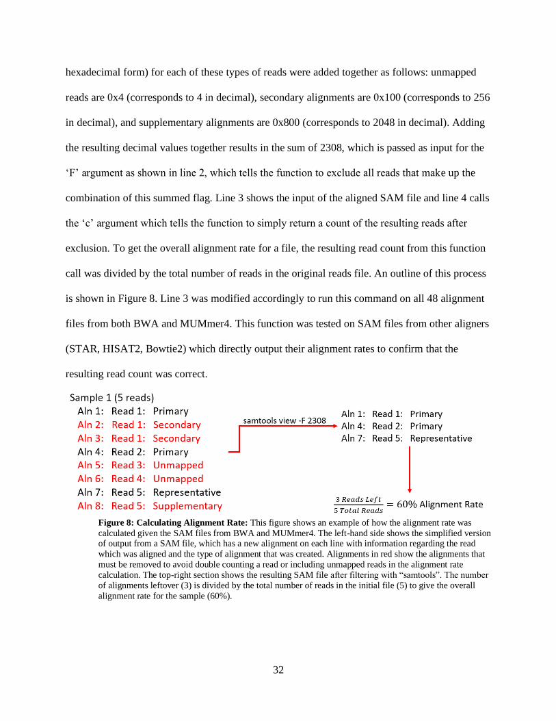
hexadecimal form) for each of these types of reads were added together as follows: unmapped

reads are 0x4 (corresponds to 4 in decimal), secondary alignments are 0x100 (corresponds to 256

in decimal), and supplementary alignments are 0x800 (corresponds to 2048 in decimal). Adding

the resulting decimal values together results in the sum of 2308, which is passed as input for the

‘F’ argument as shown in line 2, which tells the function to exclude all reads that make up the

combination of this summed flag. Line 3 shows the input of the aligned SAM file and line 4 calls

the ‘c’ argument which tells the function to simply return a count of the resulting reads after

exclusion. To get the overall alignment rate for a file, the resulting read count from this function

call was divided by the total number of reads in the original reads file. An outline of this process

is shown in Figure 8. Line 3 was modified accordingly to run this command on all 48 alignment

files from both BWA and MUMmer4. This function was tested on SAM files from other aligners

(STAR, HISAT2, Bowtie2) which directly output their alignment rates to confirm that the

resulting read count was correct.

Figure 8: Calculating Alignment Rate: This figure shows an example of how the alignment rate was

calculated given the SAM files from BWA and MUMmer4. The left-hand side shows the simplified version of output from a SAM file, which has a new alignment on each line with information regarding the read

which was aligned and the type of alignment that was created. Alignments in red show the alignments that

must be removed to avoid double counting a read or including unmapped reads in the alignment rate

calculation. The top-right section shows the resulting SAM file after filtering with “samtools”. The number

of alignments leftover (3) is divided by the total number of reads in the initial file (5) to give the overall

alignment rate for the sample (60%).

33

Transcriptome Coverage

Attempts were made using a variety of tools to assess the completeness of the overall

transcriptome of E. necator. Coverage of the transcriptome was calculated to be used as an

extrapolation of the alignment rate variable to determine if aligners had a certain bias as to what

type of genes were able to be mapped to the reference genome. The goal for calculating

transcriptome coverage was to combine the aligned reads from all 48 samples for a given aligner

and use these results to determine an aligners maximum coverage of the transcriptome given

reads from 48 “replicates”. This would remove the outside variable of a given sample not

containing (or having a low expression) of a particular gene because the sample was grown in a

distinctly different geographical location. The following is a breakdown of the attempts at

calculating transcriptome coverage for E. necator.

BUSCO

The first attempt at determining transcriptome coverage was to use the Benchmarking

Universal Single-Copy Orthologs tool (or BUSCO) (Simão et al., 2015). The BUSCO tool works

to identify “BUSCOs”, which are often core metabolic genes that exist in nearly all (>90%)

species in each phylogenetic clade, that appear in a sequenced sample file. For example, the

clade of all Leotiomycetes, the class level of which E. necator belongs to, has 3,234 BUSCOs

that have been identified which are “universal” to all species that are classified under

Leotiomycetes. A resulting run reports the number of BUSCOs discovered in a given sample that

are fully intact (“Complete”), partially found (“Fragmented”), or missing from the sample

entirely. BUSCO is often used as a measure for completeness by adding the “Complete” and

“Fragmented” percentages to make sure that a newly assembled genome/transcriptome has a

majority of the nearly universal core genes. As input, BUSCO requires a FASTA file created

34

from the SAM files given from an alignment. To first convert the SAM files to a sorted BAM

file, the “samtools” functions ‘view’ and ‘sort’ were used (see Supplementary B13). To convert

from BAM to FASTA, the “samtools” function ‘fasta’ was used. To run BUSCO (v4.0.5), the

following commands must be run first:

Line 1 adds the ‘myconfig.ini’ file, which is the configuration file created upon installing

BUSCO, to the environment variable “BUSCO_CONFIG_FILE”. Line 2 does a similar task by

adding the configuration directory for the tool Augustus (installed alongside BUSCO) to the

environment variable “AUGUSTUS_CONFIG_FILE”. Both calls are required for BUSCO and

Augustus to run properly. To run BUSCO on the resulting FASTA files from an alignment, the

following command was used:

Line 1 calls the “busco” function from the appropriate directory followed by the inputted

FASTA file for argument ‘i’ on line 2 and the name of the outputted directory and files to be

created for argument ‘o’ on line 3. Line 4 tells the function to run in “transcriptome” mode (as

Adding Configuration Files to Environment Variables for BUSCO:

1) export BUSCO_CONFIG_FILE=/path_to_file/myconfig.ini

2) export AUGUSTUS_CONFIG_FILE=/path_to_config/

Running BUSCO on A01.fa:

1) /path_to_BUSCO/busco \

2) -i A01.fa \

3) -o A01_BUSCO \

4) -m tran \

5) -l leotiomycetes_odb10 \

6) -c 5

35

the FASTA files are created from aligned RNA-seq reads) by passing ‘tran’ as input for

argument ‘m’. Line 5 chooses the correct database of BUSCOs to compare to, in this case

“leotiomycetes_odb10”, and uses it as input for argument ‘l’. To run BUSCO using multiple

cores, the number of cores to be used is passed in as input for argument ‘c’.

Exonerate

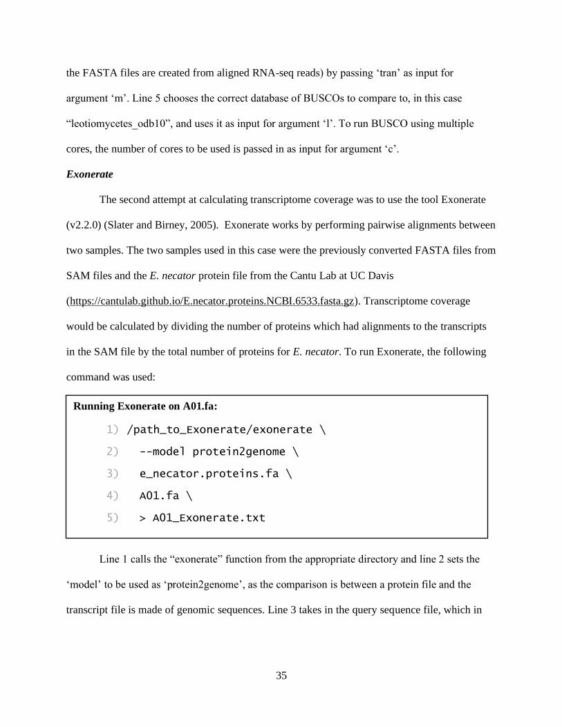
The second attempt at calculating transcriptome coverage was to use the tool Exonerate

(v2.2.0) (Slater and Birney, 2005). Exonerate works by performing pairwise alignments between

two samples. The two samples used in this case were the previously converted FASTA files from

SAM files and the E. necator protein file from the Cantu Lab at UC Davis

(https://cantulab.github.io/E.necator.proteins.NCBI.6533.fasta.gz). Transcriptome coverage

would be calculated by dividing the number of proteins which had alignments to the transcripts

in the SAM file by the total number of proteins for E. necator. To run Exonerate, the following

command was used:

Line 1 calls the “exonerate” function from the appropriate directory and line 2 sets the

‘model’ to be used as ‘protein2genome’, as the comparison is between a protein file and the

transcript file is made of genomic sequences. Line 3 takes in the query sequence file, which in

Running Exonerate on A01.fa:

1) /path_to_Exonerate/exonerate \

2) --model protein2genome \

3) e_necator.proteins.fa \

4) A01.fa \

5) > A01_Exonerate.txt

36

this case is the protein file from the Cantu Labs, and line 4 takes in the target sequence file,

which is the FASTA file of aligned reads. Line 5 redirects output from Exonerate into a file.

HTSeq

The third attempt at calculating transcriptome coverage used the python package HTSeq

(v0.11.3) (Anders, Pyl, and Huber, 2014). The “count” function from the HTSeq package

requires an alignment file and a feature file in GTF format, which lists the name and position of

all features (in this case transcripts) in the reference species. “HTSeq-count” works by counting

the number of reads in the alignment file that correspond to a given transcript in the feature file.

To calculate transcriptome coverage from these results, the number of transcripts that had a

count of at least one would be divided by the total number of transcripts in the feature file. In this

case, the feature file being used is the E. necator GFF file from the Cantu Lab at UC Davis

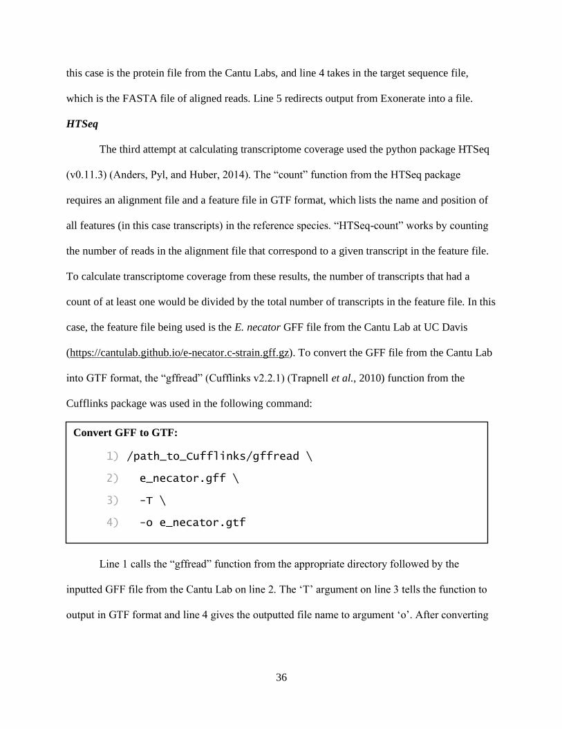
(https://cantulab.github.io/e-necator.c-strain.gff.gz). To convert the GFF file from the Cantu Lab

into GTF format, the “gffread” (Cufflinks v2.2.1) (Trapnell et al., 2010) function from the

Cufflinks package was used in the following command:

Line 1 calls the “gffread” function from the appropriate directory followed by the

inputted GFF file from the Cantu Lab on line 2. The ‘T’ argument on line 3 tells the function to

output in GTF format and line 4 gives the outputted file name to argument ‘o’. After converting

Convert GFF to GTF:

1) /path_to_Cufflinks/gffread \

2) e_necator.gff \

3) -T \

4) -o e_necator.gtf

37

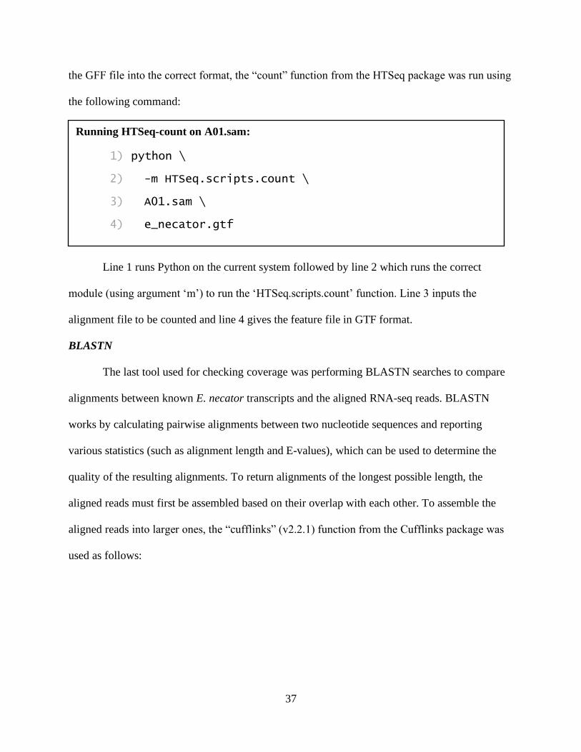
the GFF file into the correct format, the “count” function from the HTSeq package was run using

the following command:

Line 1 runs Python on the current system followed by line 2 which runs the correct

module (using argument ‘m’) to run the ‘HTSeq.scripts.count’ function. Line 3 inputs the

alignment file to be counted and line 4 gives the feature file in GTF format.

BLASTN

The last tool used for checking coverage was performing BLASTN searches to compare

alignments between known E. necator transcripts and the aligned RNA-seq reads. BLASTN

works by calculating pairwise alignments between two nucleotide sequences and reporting

various statistics (such as alignment length and E-values), which can be used to determine the

quality of the resulting alignments. To return alignments of the longest possible length, the

aligned reads must first be assembled based on their overlap with each other. To assemble the

aligned reads into larger ones, the “cufflinks” (v2.2.1) function from the Cufflinks package was

used as follows:

Running HTSeq-count on A01.sam:

1) python \

2) -m HTSeq.scripts.count \

3) A01.sam \

4) e_necator.gtf

38

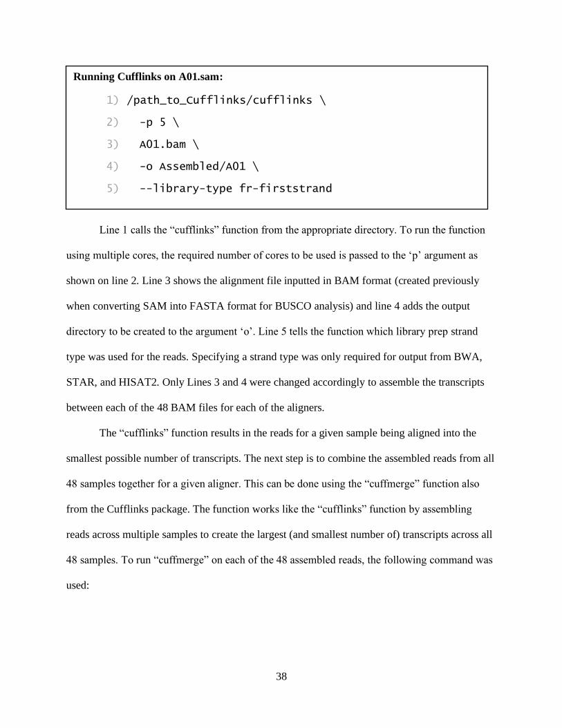
Line 1 calls the “cufflinks” function from the appropriate directory. To run the function

using multiple cores, the required number of cores to be used is passed to the ‘p’ argument as

shown on line 2. Line 3 shows the alignment file inputted in BAM format (created previously

when converting SAM into FASTA format for BUSCO analysis) and line 4 adds the output

directory to be created to the argument ‘o’. Line 5 tells the function which library prep strand

type was used for the reads. Specifying a strand type was only required for output from BWA,

STAR, and HISAT2. Only Lines 3 and 4 were changed accordingly to assemble the transcripts

between each of the 48 BAM files for each of the aligners.

The “cufflinks” function results in the reads for a given sample being aligned into the

smallest possible number of transcripts. The next step is to combine the assembled reads from all

48 samples together for a given aligner. This can be done using the “cuffmerge” function also

from the Cufflinks package. The function works like the “cufflinks” function by assembling

reads across multiple samples to create the largest (and smallest number of) transcripts across all

48 samples. To run “cuffmerge” on each of the 48 assembled reads, the following command was

used:

Running Cufflinks on A01.sam:

1) /path_to_Cufflinks/cufflinks \

2) -p 5 \

3) A01.bam \

4) -o Assembled/A01 \

5) --library-type fr-firststrand

39

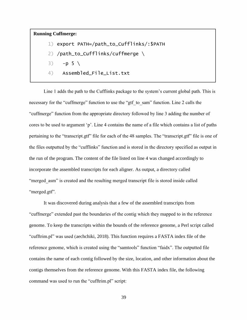
Line 1 adds the path to the Cufflinks package to the system’s current global path. This is

necessary for the “cuffmerge” function to use the “gtf_to_sam” function. Line 2 calls the

“cuffmerge” function from the appropriate directory followed by line 3 adding the number of

cores to be used to argument ‘p’. Line 4 contains the name of a file which contains a list of paths

pertaining to the “transcript.gtf” file for each of the 48 samples. The “transcript.gtf” file is one of

the files outputted by the “cufflinks” function and is stored in the directory specified as output in

the run of the program. The content of the file listed on line 4 was changed accordingly to

incorporate the assembled transcripts for each aligner. As output, a directory called

“merged_asm” is created and the resulting merged transcript file is stored inside called

“merged.gtf”.

It was discovered during analysis that a few of the assembled transcripts from

“cuffmerge” extended past the boundaries of the contig which they mapped to in the reference

genome. To keep the transcripts within the bounds of the reference genome, a Perl script called

“cufftrim.pl” was used (aechchiki, 2018). This function requires a FASTA index file of the

reference genome, which is created using the “samtools” function “faidx”. The outputted file

contains the name of each contig followed by the size, location, and other information about the

contigs themselves from the reference genome. With this FASTA index file, the following

command was used to run the “cufftrim.pl” script:

Running Cuffmerge:

1) export PATH=/path_to_Cufflinks/:$PATH

2) /path_to_Cufflinks/cuffmerge \

3) -p 5 \

4) Assembled_File_List.txt

40

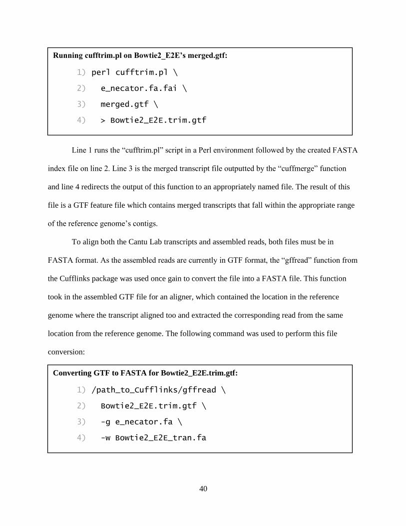
Line 1 runs the “cufftrim.pl” script in a Perl environment followed by the created FASTA

index file on line 2. Line 3 is the merged transcript file outputted by the “cuffmerge” function

and line 4 redirects the output of this function to an appropriately named file. The result of this

file is a GTF feature file which contains merged transcripts that fall within the appropriate range

of the reference genome’s contigs.

To align both the Cantu Lab transcripts and assembled reads, both files must be in

FASTA format. As the assembled reads are currently in GTF format, the “gffread” function from

the Cufflinks package was used once gain to convert the file into a FASTA file. This function

took in the assembled GTF file for an aligner, which contained the location in the reference

genome where the transcript aligned too and extracted the corresponding read from the same

location from the reference genome. The following command was used to perform this file

conversion:

Running cufftrim.pl on Bowtie2_E2E’s merged.gtf:

1) perl cufftrim.pl \

2) e_necator.fa.fai \

3) merged.gtf \

4) > Bowtie2_E2E.trim.gtf

Converting GTF to FASTA for Bowtie2_E2E.trim.gtf:

1) /path_to_Cufflinks/gffread \

2) Bowtie2_E2E.trim.gtf \

3) -g e_necator.fa \

4) -w Bowtie2_E2E_tran.fa

41

Line 1 calls the “gffread” function from the appropriate directory followed by the

inputted GTF transcript file on line 2. Line 3 assigns the reference genome to the argument ‘g’

and line 4 adds the output file to be created to argument ‘w’. Lines 2 and 4 were modified

accordingly to create FASTA files for transcripts from each of the aligners.

To align the known transcripts of E. necator to the transcripts assembled from an aligner,

a database must be created from the assembled transcript file. The “makeblastdb” function from

the BLAST+ package (v2.5.0+) (Camacho et al., 2009) was used to create the database with the

following command:

Line 1 calls the “makeblastdb” function from the appropriate directory followed by the

inputted FASTA file added to argument ‘in’ on line 2. Line 3 is required if the input is in FASTA

format for the function to correctly pull out the sequence ID’s from the header of each entry.

Line 4 tells the function which type of database is to be created by adding ‘nucl’ (for nucleotide)

to the argument ‘dbtype’.

After creating the database of aligned transcripts, the BLAST search was performed

using the transcript file taken from the Cantu Lab at UC Davis as a query

(https://cantulab.github.io/E.necator.transcripts.NCBI.6533.fasta.gz). The BLAST search was

performed using the following command:

Creating a BLAST Database from Bowtie2_E2E_tran.fa:

1) /path_to_BLAST+/makeblastdb \

2) -in Bowtie2_E2E_tran.fa \

3) -parse_seqids \

4) -dbtype nucl

42

Line 1 calls the “blastn” function from the appropriate directory. Line 2 assigns the

FASTA file of transcripts from the Cantu Lab as the ‘query’ argument. Line 3 requires the name

of the FASTA file from which the database was created provided as input for the ‘db’ argument’

and line 4 assigns the file to be created as output to the ‘out’ argument. Line 5 tells the function

to only output the single best alignment per transcript in the query by adding a 1 to the argument

‘max_target_seqs’. Line 6 tells the function which types of the information to report in the

outputted TSV (format notified by the ‘6’): query name, query length, target name, target length,

E-value for the alignment, length of the alignment, and query coverage, respectively. Lines 3 and

4 were modified accordingly to run the BLASTN function against databases for the other 6

aligners.

Transcriptome coverage was then calculated from the output of the BLASTN function by

counting the number of lines in the output file and dividing by the total number of transcripts in

the Cantu Lab transcript file. Each line in the output corresponded to a single alignment and

there was no double counting of transcripts as only one alignment was returned per transcript.

Additionally, the transcriptome coverage was calculated similarly for various cutoffs based on

minimum values for the overall alignment length.

Running BLASTN with Bowtie_E2E_tran.fa Database:

1) /path_to_BLAST+/blastn \

2) -query e_necator.transcript.fa \

3) -db Bowtie_E2E_tran.fa \

4) -out Bowtie_E2E.tsv \

5) -max_target_seqs 1

6) -outfmt “6 qacc qlen sacc slen evalue length qcovs”

43

Checking for Gene Bias

BLAST+ results were then used to check whether there was any bias as to which type of

genes were unable to be mapped by an aligner. Code was written to extract from the Cantu Lab

transcript file those genes that did not have at least a partial hit in the BLAST+ output for an

aligner. These genes which were not found were submitted in FASTA file format to eggNOG-

mapper v2 to classify the missing genes based on their annotation results (Huerta-Cepas et al.,

2017). Bias was determined for each aligner by examining the proportion of missing genes

which were reported to belong to each Clusters of Orthologous Groups of proteins (COG)

category assigned by EggNOG-mapper (Tatusov et al., 2000).

Results

Initial Quality Assessment

Raw reads for all samples were initially checked for overall quality using FastQC. The

average number of raw reads per sample was 3,677,174. The initial results from FastQC on these

reads displayed poor quality for each of the 48 samples of E. necator. Each of the 48 samples

had similar distributions for all results outputted by FastQC so Figure 9 shows the output for a

representative sample, split_A01.fq. Examining the “Per base sequence quality” resulted in a

large proportion of the bases having low quality scores, particularly near the 3’-end of the reads,

given the large portions of the box plot distributions (one plot created for each base position)

being in the < 20 Q-score area (red in color) of the chart in Figure 9A. As a Q-score of 20 was

the desired value and indicates a 99% accurate base call at a given position, any score below this

value would have an incorrect base call > 1% of the time and therefore would need to be

trimmed. A second important finding from examining the initial FastQC tests was the

44

particularly high N-content at position 6 of all reads as seen in Figure 9B. The results from the

N-content distribution showed that in nearly 45% of the reads an ‘N’ was placed at the 6th

position due to the sequencer being unable to determine a base for this position. Due to the large

ambiguity at this position, it was this finding that resulted in the decision to remove the 6th base

from the reads along with the first 5 bases which corresponded to the sample barcodes. Initial

results also showed a slight bias across the length of each read in the calling of A’s and T’s as

seen in Figure 9C. Ideally, each of the bases should be assigned roughly 25% of the time (a ¼

chance due to their being 4 nucleotides), so there was a slight overrepresentation of A’s and T’s

(approximately 30%) throughout all 48 samples. In contrast, bases 1 through 6 all had abnormal

base-calling distributions, which was to be expected as the same 5 bases were placed at the

beginning of each read for sample identification. This led to a nearly 100% calling of a given

base for the first 5 positions, which further solidified the reason to remove these bases from each

of the reads. Further, a higher percentage of the reads had low GC content, indicated by the

leftmost peak of the red curve in Figure 9D showing the “Per sequence GC content”. This peak

most likely came from an overabundance of poly-A tails being represented in the dataset as reads

of all (or large portions of) A’s would record GC contents of ~0%, resulting in the peak for a

high number of low GC reads. Ideally, the GC content distribution across all reads should follow

a normal distribution (displayed by the blue curve in Figure 9D).

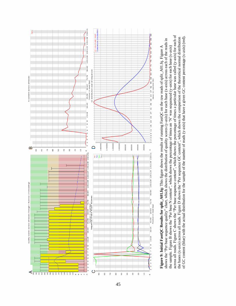
45

Fig

ure

9:

Init

ial

Fast

QC

Resu

lts

for s

pli

t_A

01.f

q:

This

fig

ure

sho

ws

the

resu

lts

of

run

nin

g F

astQ

C o

n t

he

raw

rea

ds

of

spli

t_A

01.f

q. F

igure

A

sho

ws

the

“Per

bas

e se

quen

ce q

ual

ity”

char

t, w

hic

h s

ho

ws

the

dis

trib

uti

on o

f q

ual

ity

sco

res

(y-a

xis

) fo

r ea

ch b

ase

(x-a

xis

) ac

ross

eac

h o

f th

e re

ads

in

the

sam

ple

. F

igure

B s

how

s th

e “P

er b

ase

N c

on

tent”

, w

hic

h s

ho

ws

the

per

centa

ge

of

tim

es a

n ‘

N’

was

seq

uen

ced (

y-a

xis

) fo

r ea

ch b

ase

(x-a

xis

) ac

ross

all

rea

ds.

Fig

ure

C s

how

s th

e “P

er b

ase

seq

uen

ce c

onte

nt”

, w

hic

h s

ho

ws

the

per

cen

tag

e o

f ti

mes

a par

ticu

lar

bas

e w

as c

alle

d (

y-a

xis

) fo

r ea

ch o

f

the

bas

es (

x-a

xis

) ac

ross

all

rea

ds.

Fig

ure

D s

ho

ws

the

“Per

seq

uen

ce G

C c

on

ten

t”, w

hic

h s

ho

ws

the

com

par

ison o

f th

e th

eore

tica

l norm

al d

istr

ibuti

on

of

GC

conte

nt

(blu

e) w

ith t

he

actu

al d

istr

ibu

tio

n f

or

the

sam

ple

of

the

num

ber

of

read

s (y

-axis

) th

at h

ave

a giv

en G

C c

onte

nt

per

centa

ge

(x-a

xis

) (r

ed).

46

FASTX Clean Up

Raw reads were then trimmed by removing the 5 base pair barcodes and high N-content

base at position 6 from the 5’-end as well as removing low quality bases from the 3’-end. After

quality trimming, any read below 100 base pairs was removed from the sample. Running FastQC

on the trimmed reads showed much cleaner reads for all samples. All samples had the same

general results so the FastQC results of a single sample, split_A01.fq, can be seen in Figure 10.

The overall distribution of quality scores was significantly improved by removal of low-quality

reads as seen in Figure 10A by the boxplot distributions appearing primarily in the “> 20 Q-

score”-region. The drastic increase in quality was most likely since FASTX had removed a large

percentage of reads from each of the samples. After trimming, the average number of reads

remaining across all samples was 741,219. This resulted in an average of 20.04% of reads left

after quality control. The percentage of N’s appearing throughout the reads was also reduced,

shown in Figure 10B, so that no sample even had over 5% of N’s at a given base position. The

sequence content on the 5’-ends was improved by removing the barcodes (as shown in Figure

10C), which lessened the overrepresented base calling as the same 5 bases were attached to every

read for a given sample. The slight bias in A and T overrepresentation was also present post-

trimming but was not determined to have much of an impact on alignment results downstream.

Further, the GC content across all the reads post-trimming was much more normally distributed

as shown in Figure 10D, most likely due to the removal of low-quality poly-A tails. Taking all of

these quality control results into consideration, it was determined that the reads were of a good

enough quality to continue with alignment.

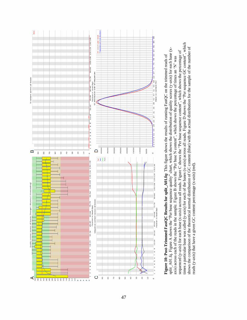
47

Fig

ure

10:

Post

-Tri

mm

ed

Fast

QC

Resu

lts

for s

pli

t_A

01.f

q:

This

fig

ure

sh

ow

s th

e re

sult

s o

f ru

nnin

g F

astQ

C o

n t

he

trim

med

rea

ds

of

spli

t_A

01.f

q. F

igure

A s

how

s th

e “P

er b

ase

seq

uen

ce q

ual

ity”

char

t, w

hic

h s

ho

ws

the

dis

trib

uti

on

of

qual

ity s

core

s (y

-axis

) fo

r ea

ch b

ase

(x-

axis

) ac

ross

eac

h o

f th

e re

ads

in t

he

sam

ple

. F

igu

re B

sh

ow

s th

e “P

er b

ase

N c

onte

nt”

, w

hic

h s

ho

ws

the

per

centa

ge

of

tim

es a

n ‘

N’

was

seq

uen

ced (

y-a

xis

) fo

r ea

ch b

ase

(x-a

xis

) ac

ross

all

rea

ds.

Fig

ure

C s

ho

ws

the

“Per

bas

e se

quen

ce c

onte

nt”

, w

hic

h s

how

s th

e per

centa

ge

of

tim

es a

par

ticu

lar

bas

e w

as c

alle

d (

y-a

xis

) fo

r ea

ch o

f th

e b

ases

(x

-ax

is)

acro

ss a

ll r

ead

s. F

igu

re D

sh

ow

s th

e “P

er s

equen

ce G

C c

onte

nt”

, w

hic

h

sho

ws

the

com

par

ison o

f th

e th

eore

tica

l n

orm

al d

istr

ibu

tio

n o

f G

C c

onte

nt

(blu

e) w

ith

th

e ac

tual

dis

trib

uti

on f

or

the

sam

ple

of

the

num

ber

of

read

s (y

-ax

is)

that

hav

e a

giv

en G

C c

onte

nt

per

cen

tag

e (x

-axis

) (r

ed).

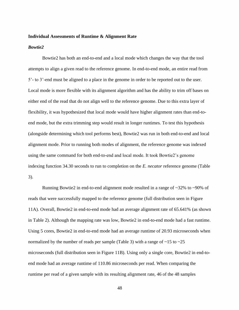
48

Individual Assessments of Runtime & Alignment Rate

Bowtie2

Bowtie2 has both an end-to-end and a local mode which changes the way that the tool

attempts to align a given read to the reference genome. In end-to-end mode, an entire read from

5’- to 3’-end must be aligned to a place in the genome in order to be reported out to the user.

Local mode is more flexible with its alignment algorithm and has the ability to trim off bases on

either end of the read that do not align well to the reference genome. Due to this extra layer of

flexibility, it was hypothesized that local mode would have higher alignment rates than end-to-

end mode, but the extra trimming step would result in longer runtimes. To test this hypothesis

(alongside determining which tool performs best), Bowtie2 was run in both end-to-end and local

alignment mode. Prior to running both modes of alignment, the reference genome was indexed

using the same command for both end-to-end and local mode. It took Bowtie2’s genome

indexing function 34.30 seconds to run to completion on the E. necator reference genome (Table

3).

Running Bowtie2 in end-to-end alignment mode resulted in a range of ~32% to ~90% of

reads that were successfully mapped to the reference genome (full distribution seen in Figure

11A). Overall, Bowtie2 in end-to-end mode had an average alignment rate of 65.641% (as shown

in Table 2). Although the mapping rate was low, Bowtie2 in end-to-end mode had a fast runtime.

Using 5 cores, Bowtie2 in end-to-end mode had an average runtime of 20.93 microseconds when

normalized by the number of reads per sample (Table 3) with a range of ~15 to ~25

microseconds (full distribution seen in Figure 11B). Using only a single core, Bowtie2 in end-to-

end mode had an average runtime of 110.86 microseconds per read. When comparing the

runtime per read of a given sample with its resulting alignment rate, 46 of the 48 samples

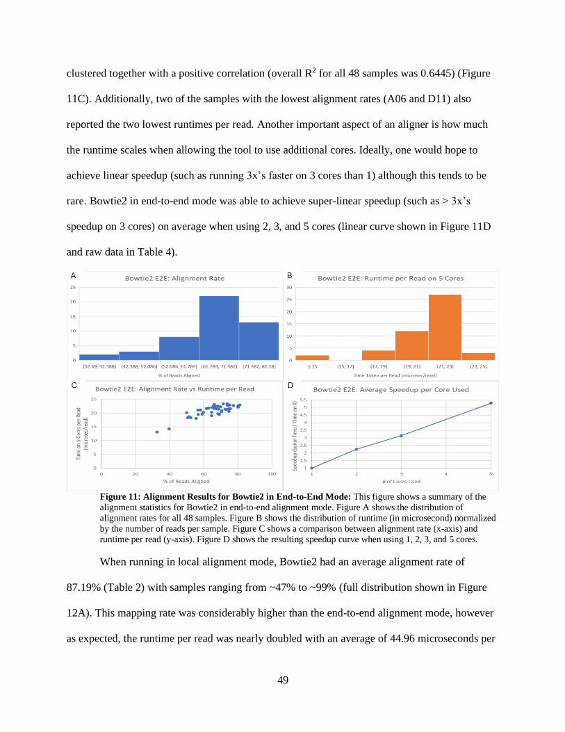
49

clustered together with a positive correlation (overall R2 for all 48 samples was 0.6445) (Figure

11C). Additionally, two of the samples with the lowest alignment rates (A06 and D11) also

reported the two lowest runtimes per read. Another important aspect of an aligner is how much

the runtime scales when allowing the tool to use additional cores. Ideally, one would hope to

achieve linear speedup (such as running 3x’s faster on 3 cores than 1) although this tends to be

rare. Bowtie2 in end-to-end mode was able to achieve super-linear speedup (such as > 3x’s

speedup on 3 cores) on average when using 2, 3, and 5 cores (linear curve shown in Figure 11D

and raw data in Table 4).

Figure 11: Alignment Results for Bowtie2 in End-to-End Mode: This figure shows a summary of the

alignment statistics for Bowtie2 in end-to-end alignment mode. Figure A shows the distribution of

alignment rates for all 48 samples. Figure B shows the distribution of runtime (in microsecond) normalized

by the number of reads per sample. Figure C shows a comparison between alignment rate (x-axis) and

runtime per read (y-axis). Figure D shows the resulting speedup curve when using 1, 2, 3, and 5 cores.

When running in local alignment mode, Bowtie2 had an average alignment rate of

87.19% (Table 2) with samples ranging from ~47% to ~99% (full distribution shown in Figure

12A). This mapping rate was considerably higher than the end-to-end alignment mode, however

as expected, the runtime per read was nearly doubled with an average of 44.96 microseconds per

50

read using 5 cores (Table 3). This resulted in a range of runtimes from ~30 to ~54 microseconds

per read (full distribution seen in Figure 12B). Using only a single core, Bowtie2’s local

alignment mode had an average runtime per read of 226.63 microseconds (Table 3), also doubled

from end-to-end mode’s single core runtime. When comparing the runtime per read against the

alignment rate, Bowtie2 in local alignment mode also showed tight clustering for 46 of the 48

samples with an a highly positive correlation (R2 = 0.9495) (Figure 12C). Additionally, the two

samples in local mode which achieved the lowest alignment rates and lowest runtime per read

(A06 and D11) were the same two samples which end-to-end mode had a difficult time mapping

to the reference genome. Also, like end-to-end mode, Bowtie2’s local alignment mode achieved

linear speedup on average when using 2, 3, and 5 cores (linear curve seen in Figure 12D and raw

data in Table 4).

Figure 12: Alignment Results for Bowtie2 in Local Mode: This figure shows a summary of the

alignment statistics for Bowtie2 in local alignment mode. Figure A shows the distribution of alignment

rates for all 48 samples. Figure B shows the distribution of runtime (in microsecond) normalized by the

number of reads per sample. Figure C shows a comparison between alignment rate (x-axis) and runtime per

read (y-axis). Figure D shows the resulting speedup curve when using 1, 2, 3, and 5 cores.

51

BWA

Building the reference genome index with BWA took roughly the same amount of time

as Bowtie2 with a time of 33.45 seconds (Table 3). Aligning the samples with BWA saw a large

percentage of the reads being mapped to the reference genome. On average, 87.41% of a

sample’s reads were successfully aligned (Table 2) with a range of ~47% to ~99% and a nearly

identical distribution as Bowtie2 when run using local mode (Figure 13A). BWA achieved the

best average alignment when compared to all other aligners tested. The runtime per read using

BWA was fast using on average 24.04 microseconds per read with 5 cores and 104.50

microseconds per read with a single core (Table 3). The range of runtimes on 5 cores had a very

tight distribution with a range of ~21 to ~28 microseconds per read (Figure 13B). Like both

alignment modes for Bowtie2, BWA had 46 of the 48 samples cluster tightly together when

comparing the runtime per read and alignment rates (Figure 13C). Overall, there was only a

slightly positive correlation between the two variables (R2 = 0.2286). Again, the two samples

that recorded the lowest alignment rates (A06 and D11) were the same as those identified by

Bowtie2. When analyzing the speedup curve, BWA achieved nearly linear speedup on average

when using 2 cores, but less than linear using 3 and 5 cores (linear curve seen in Figure 13D and

raw data in Table 4).

52

Figure 13: Alignment Results for BWA: This figure shows a summary of the alignment statistics for

BWA. Figure A shows the distribution of alignment rates for all 48 samples. Figure B shows the distribution of runtime (in microsecond) normalized by the number of reads per sample. Figure C shows a

comparison between alignment rate (x-axis) and runtime per read (y-axis). Figure D shows the resulting

speedup curve when using 1, 2, 3, and 5 cores.

HISAT2

When compared to the other aligners, HISAT2 had the second fastest pre-processing time

by building the reference genome index in 25.82 seconds (Table 3). Aligning with HISAT2 saw

extremely fast runtimes paired with lower alignment rates. On average, only 66.43% of a

sample’s reads were successfully mapped to the reference genome when using HISAT2 (Table

2). Alignment rates ranged from ~32% to ~86% leading to a rather large distribution (Figure

14A). In contrast to this wide spread of alignment rates, the runtimes for HISAT2 were quite fast

with a very tight range. On average, the runtime per read using 1 core was 37.81 microseconds

and using 5 cores was 8.28 microseconds (Table 3) with a range of ~6 to ~11 microseconds

(Figure 14B). The runtimes reported by HISAT2 were among the fastest runtimes for any aligner

tested. When comparing the alignment rate against the runtime per read, no correlation (R2 =

0.0876) was found partially due to the large range of alignment rates obtained (Figure 14C).

53

Once again, the two samples that reported the two lowest alignment rates, and the two shortest

runtimes per read, (A06 and D11) were the same reported by previous tools. Similar to BWA’s

speedup curve, HISAT2 performed best using 2 cores (super-linear speedup on average) when

compared with using 3 and 5 cores, which both achieved slightly less than linear speedup on

average (curve seen in Figure 14D and raw data in Table 4).

Figure 14: Alignment Results for HISAT2: This figure shows a summary of the alignment statistics for

HISAT2. Figure A shows the distribution of alignment rates for all 48 samples. Figure B shows the distribution of runtime (in microsecond) normalized by the number of reads per sample. Figure C shows a

comparison between alignment rate (x-axis) and runtime per read (y-axis). Figure D shows the resulting

speedup curve when using 1, 2, 3, and 5 cores.

MUMmer4

One place where MUMmer4 performed substantially better than other aligners was its

ability to build the genome index very quickly. MUMmer4 only required 7.96 seconds to process

E. necator’s genome, approximately 3x’s faster than the second fastest aligner HISAT2 (Table

3). Although being the cause of the most trouble due to having incorrect output formats,

MUMmer4 had good results for both alignment rates and runtimes. The average alignment rate

54

with MUMmer4 was 77.94% (Table 2) with a range of ~40% to ~93% (Figure 15A). Although

this range is rather large, a large proportion of the samples (46 of the 48) achieved > 60%

alignment rates with the two samples < 60% being sample A06 and D11, the same ones reported

by previous aligners as being troublesome. When using only a single core, MUMmer4 had an

average runtime per read of 186.90 microseconds. Although being one of the longer runtimes on

1 core, MUMmer4 scaled well by using more cores as made evident by the average runtime per

read on 5 cores being 37.70 microseconds (Table 3) with a range of ~31 to ~43 microseconds

(Figure 15B). In addition, the linear speedup curve for MUMmer4 showed the aligner

performing at super-linear speedup using 2 cores and linear speedup using 3 and 5 cores (curve

in Figure 15D and raw data in Table 4). MUMmer4 showed tight clustering on both axes and a

slightly positive correlation (R2 = 0.2722) between the runtime per read with the alignment rate

(Figure 15C). As stated earlier, the two samples with the fastest runtime and lowest alignment

rate were A06 and D11.

55

Figure 15: Alignment Results for MUMmer4: This figure shows a summary of the alignment statistics

for MUMmer4. Figure A shows the distribution of alignment rates for all 48 samples. Figure B shows the distribution of runtime (in microsecond) normalized by the number of reads per sample. Figure C shows a

comparison between alignment rate (x-axis) and runtime per read (y-axis). Figure D shows the resulting

speedup curve when using 1, 2, 3, and 5 cores.

STAR

Pre-processing with STAR involved building the uncompressed suffix array from the E.

necator reference genome, which took 80.42 seconds to build (Table 3). If STAR did not have

the option to pre-build genome index, this long runtime would negatively impact overall

runtimes as STAR had the slowest pre-processing time of all aligners (2x’s the next slowest).

However, the ability to only run this command once and call the built index in subsequent

alignments resulted in STAR having the second fastest (behind HISAT2) runtime per read using

a single core with an average time of 67.45 microseconds (Table 3). Running STAR on 5 cores

resulted in an average time of 22.89 microseconds per read (Table 3) and a range of ~12 to ~59

microseconds (Figure 16B). Using an increasing number of cores resulted in a logarithmic

speedup curve that was well below the ideal linear curve (Figure 16D and raw data in Table 4).

In terms of alignment rates, STAR had an average alignment rate of 78.48% across all samples

56

(Table 2) with a range of ~40% to ~93% (Figure 16A). Analyzing the correlation between

runtime per read and alignment for STAR found an overall negative relationship (R2 = 0.3904)

between the two variables (Figure 16C). Like previous aligners, STAR also reported samples

A06 and D11 with having the lowest alignment rates.

Figure 16: Alignment Results for STAR: This figure shows a summary of the alignment statistics for

STAR. Figure A shows the distribution of alignment rates for all 48 samples. Figure B shows the distribution of runtime (in microsecond) normalized by the number of reads per sample. Figure C shows a

comparison between alignment rate (x-axis) and runtime per read (y-axis). Figure D shows the resulting

speedup curve when using 1, 2, 3, and 5 cores.

TopHat2

TopHat2 has been largely replaced with HISAT2 in terms of overall tool usage and the

results from TopHat2 on E. necator show why any aligner is a much better option. Due to

TopHat2 using Bowtie2 to perform initial alignments, the pre-processing time is equivalent to

Bowtie2’s 34.30 second runtime to build the reference genome index (Table 3). When looking at

alignment rates, TopHat2 had the lowest rate among aligners by a substantial amount (3x’s less

than the next lowest). On average, TopHat2 was able to map 18.33% of a sample’s reads to the

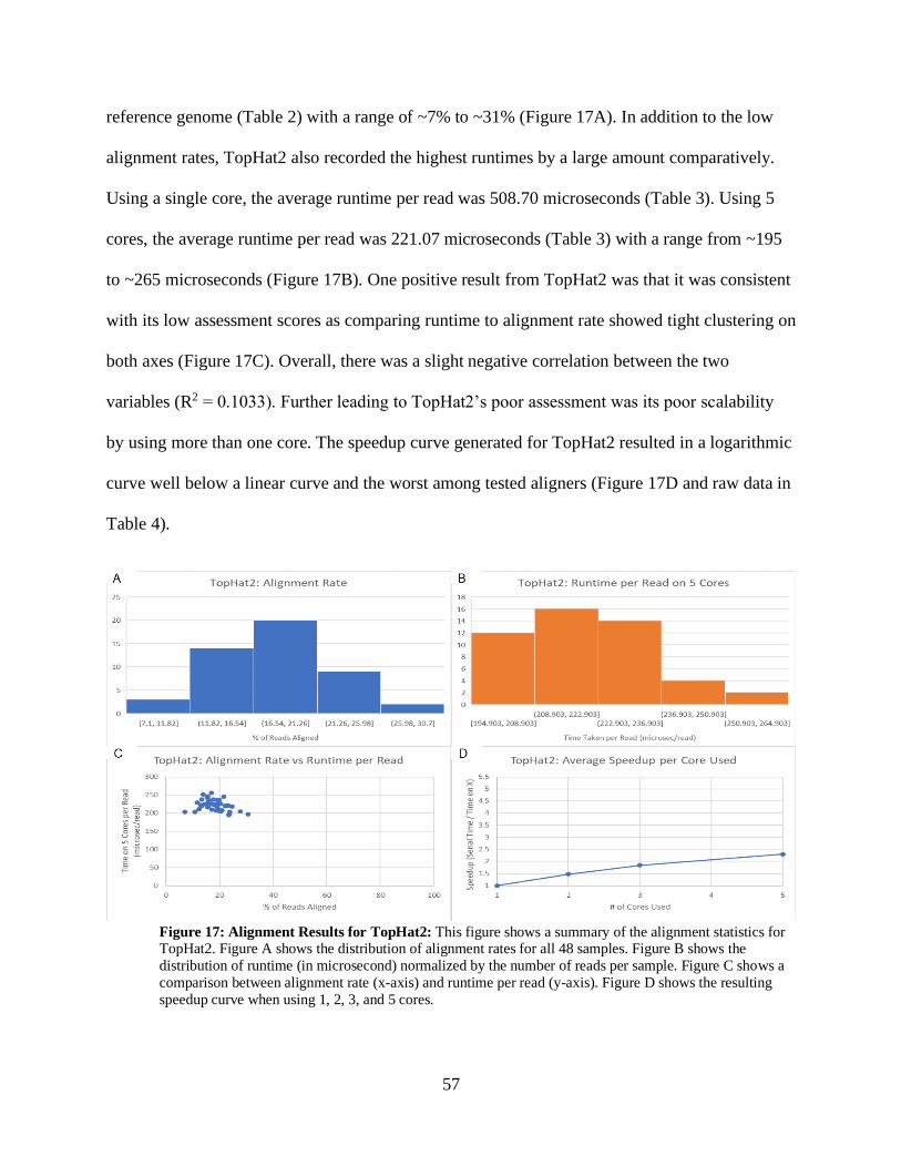
57

reference genome (Table 2) with a range of ~7% to ~31% (Figure 17A). In addition to the low

alignment rates, TopHat2 also recorded the highest runtimes by a large amount comparatively.

Using a single core, the average runtime per read was 508.70 microseconds (Table 3). Using 5

cores, the average runtime per read was 221.07 microseconds (Table 3) with a range from ~195

to ~265 microseconds (Figure 17B). One positive result from TopHat2 was that it was consistent

with its low assessment scores as comparing runtime to alignment rate showed tight clustering on

both axes (Figure 17C). Overall, there was a slight negative correlation between the two

variables (R2 = 0.1033). Further leading to TopHat2’s poor assessment was its poor scalability

by using more than one core. The speedup curve generated for TopHat2 resulted in a logarithmic

curve well below a linear curve and the worst among tested aligners (Figure 17D and raw data in

Table 4).

Figure 17: Alignment Results for TopHat2: This figure shows a summary of the alignment statistics for TopHat2. Figure A shows the distribution of alignment rates for all 48 samples. Figure B shows the

distribution of runtime (in microsecond) normalized by the number of reads per sample. Figure C shows a

comparison between alignment rate (x-axis) and runtime per read (y-axis). Figure D shows the resulting

speedup curve when using 1, 2, 3, and 5 cores.

58

Comparative Assessment of Runtime & Alignment Rate

The best way to determine which aligner performed best is by looking at a comparison of

the raw data. When examining the average alignment rate, four of the seven aligners tested had

rates greater than 75%: Bowtie2 in local alignment mode, BWA, MUMmer4, and STAR (Table

2). The aligner with the highest average alignment rate was BWA with 87.41%, followed closely

behind by Bowtie2 in local alignment mode with 87.192%. On the other end of the spectrum,

TopHat2 had the lowest average alignment rate by far with a rate of 18.33% (next lowest was

Bowtie2 in end-to-end mode with 65.64%). To further compare the aligners against each other, a

comparative boxplot chart was created where each aligner’s distribution plot was made from the

alignment rates of all 48 samples (Figure 18). A Tukey test (using Tukey’s ‘Honest Significant

Difference’ method with 95% confidence level) was also performed on the resulting distributions

to determine which of the aligner’s average alignment rates were statistically different from

another. The Tukey test resulted in four significantly distinct groups between the seven aligners.

In one group, BWA and Bowtie2 in local mode had nearly identical distributions with the highest

alignment rates. The group with the second highest rates belonged to MUMmer4 and STAR,

followed by the third group of Bowtie2 in end-to-end mode and HISAT2. The fourth and final

grouping belonged to TopHat2 by itself. All aligners, except TopHat2, identified both samples

A06 and D11 as outliers that had alignment rates well-below the rest of the samples. Like the

others, TopHat2 identified sample D11 as being an outlier below the others, but, unlike the other

aligners, identified sample A12 as an outlier with an alignment rate greater than the rest of the

samples.

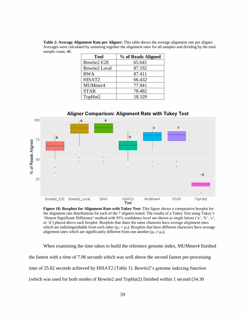
59

Table 2: Average Alignment Rate per Aligner: This table shows the average alignment rate per aligner.

Averages were calculated by summing together the alignment rates for all samples and dividing by the total

sample count, 48.

Tool % of Reads Aligned

Bowtie2 E2E 65.641

Bowtie2 Local 87.192

BWA 87.411

HISAT2 66.432

MUMmer4 77.941

STAR 78.482

TopHat2 18.329

Figure 18: Boxplots for Alignment Rate with Tukey Test: This figure shows a comparative boxplot for

the alignment rate distributions for each of the 7 aligners tested. The results of a Tukey Test using Tukey’s

‘Honest Significant Difference’ method with 95% confidence level are shown as single letters (‘a’, ‘b’, ‘c’,

or ‘d’) placed above each boxplot. Boxplots that share the same character have average alignment rates

which are indistinguishable from each other (µ1 = µ2). Boxplots that have different characters have average

alignment rates which are significantly different from one another (µ1 ≠ µ2).

When examining the time taken to build the reference genome index, MUMmer4 finished

the fastest with a time of 7.96 seconds which was well above the second fastest pre-processing

time of 25.82 seconds achieved by HISAT2 (Table 3). Bowtie2’s genome indexing function

(which was used for both modes of Bowtie2 and TopHat2) finished within 1 second (34.30

60

seconds) of BWA’s pre-processing time of 33.45 seconds. The slowest genome indexing

function belonged to STAR with a time of 80.42 seconds which was over twice as slow as the

next slowest time. When examining the average runtime per read using only a single core,

HISAT2 achieved the fastest runtime of 37.81 microseconds per read followed by STAR with

67.45 microseconds per read. The slowest runtime per read on one core belonged to TopHat2

with an average time of 508.70 microseconds which was twice as slow as the next slowest

(Bowtie2 in local mode with a time of 226.63 second). When upping the number of cores used to

five, HISAT2 still achieved the fastest runtime per read with an average time of 8.28

microseconds. Although STAR was the second fastest using one core, Bowtie2 in end-to-end

scaled better with the use of more cores to have the second fastest average runtime with a time of

20.93 microseconds per read (STAR was third with 22.89 microseconds). Once again, TopHat2

achieved the slowest runtime of 221.07 microseconds per red, which was almost five times as

slow as the next slowest aligner, Bowtie2 in local mode with a time of 44.96 microseconds per

read.

Similar to the alignment rates, a comparative boxplot with corresponding Tukey test

results was created to directly compare the runtime per reads using 5 cores for all aligners

(Figure 19). TopHat2 had by far the slowest distribution of runtimes per read and skewed results

in the initial comparison. For this reason, a second Tukey test (and resulting boxplots) was run

which excluded TopHat2 from the analysis to better estimate the differences between the other

six aligners (Figure 20). The Tukey test resulted in HISAT2 being grouped individually as the

fastest aligner, followed by the second fastest group of Bowtie2 in end-to-end mode and STAR.

Due to the large distribution of runtimes, STAR was the only aligner to appear in two distinct

groups: one as mentioned before and the second with BWA. The two slowest aligners in this

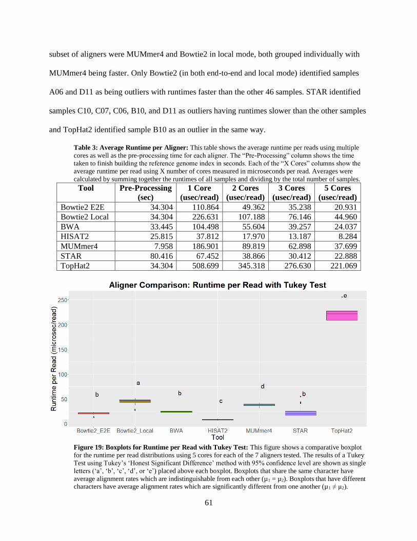
61

subset of aligners were MUMmer4 and Bowtie2 in local mode, both grouped individually with

MUMmer4 being faster. Only Bowtie2 (in both end-to-end and local mode) identified samples

A06 and D11 as being outliers with runtimes faster than the other 46 samples. STAR identified

samples C10, C07, C06, B10, and D11 as outliers having runtimes slower than the other samples

and TopHat2 identified sample B10 as an outlier in the same way.

Table 3: Average Runtime per Aligner: This table shows the average runtime per reads using multiple

cores as well as the pre-processing time for each aligner. The “Pre-Processing” column shows the time

taken to finish building the reference genome index in seconds. Each of the “X Cores” columns show the

average runtime per read using X number of cores measured in microseconds per read. Averages were

calculated by summing together the runtimes of all samples and dividing by the total number of samples.

Tool Pre-Processing

(sec)

1 Core

(usec/read)

2 Cores

(usec/read)

3 Cores

(usec/read)

5 Cores

(usec/read)

Bowtie2 E2E 34.304 110.864 49.362 35.238 20.931

Bowtie2 Local 34.304 226.631 107.188 76.146 44.960

BWA 33.445 104.498 55.604 39.257 24.037

HISAT2 25.815 37.812 17.970 13.187 8.284

MUMmer4 7.958 186.901 89.819 62.898 37.699

STAR 80.416 67.452 38.866 30.412 22.888

TopHat2 34.304 508.699 345.318 276.630 221.069

Figure 19: Boxplots for Runtime per Read with Tukey Test: This figure shows a comparative boxplot

for the runtime per read distributions using 5 cores for each of the 7 aligners tested. The results of a Tukey

Test using Tukey’s ‘Honest Significant Difference’ method with 95% confidence level are shown as single

letters (‘a’, ‘b’, ‘c’, ‘d’, or ‘e’) placed above each boxplot. Boxplots that share the same character have

average alignment rates which are indistinguishable from each other (µ1 = µ2). Boxplots that have different characters have average alignment rates which are significantly different from one another (µ1 ≠ µ2).

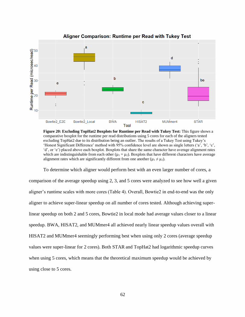
62

Figure 20: Excluding TopHat2 Boxplots for Runtime per Read with Tukey Test: This figure shows a

comparative boxplot for the runtime per read distributions using 5 cores for each of the aligners tested

excluding TopHat2 due to its distribution being an outlier. The results of a Tukey Test using Tukey’s

‘Honest Significant Difference’ method with 95% confidence level are shown as single letters (‘a’, ‘b’, ‘c’,

‘d’, or ‘e’) placed above each boxplot. Boxplots that share the same character have average alignment rates

which are indistinguishable from each other (µ1 = µ2). Boxplots that have different characters have average

alignment rates which are significantly different from one another (µ1 ≠ µ2).

To determine which aligner would perform best with an even larger number of cores, a

comparison of the average speedup using 2, 3, and 5 cores were analyzed to see how well a given

aligner’s runtime scales with more cores (Table 4). Overall, Bowtie2 in end-to-end was the only

aligner to achieve super-linear speedup on all number of cores tested. Although achieving super-

linear speedup on both 2 and 5 cores, Bowtie2 in local mode had average values closer to a linear

speedup. BWA, HISAT2, and MUMmer4 all achieved nearly linear speedup values overall with

HISAT2 and MUMmer4 seemingly performing best when using only 2 cores (average speedup

values were super-linear for 2 cores). Both STAR and TopHat2 had logarithmic speedup curves

when using 5 cores, which means that the theoretical maximum speedup would be achieved by

using close to 5 cores.

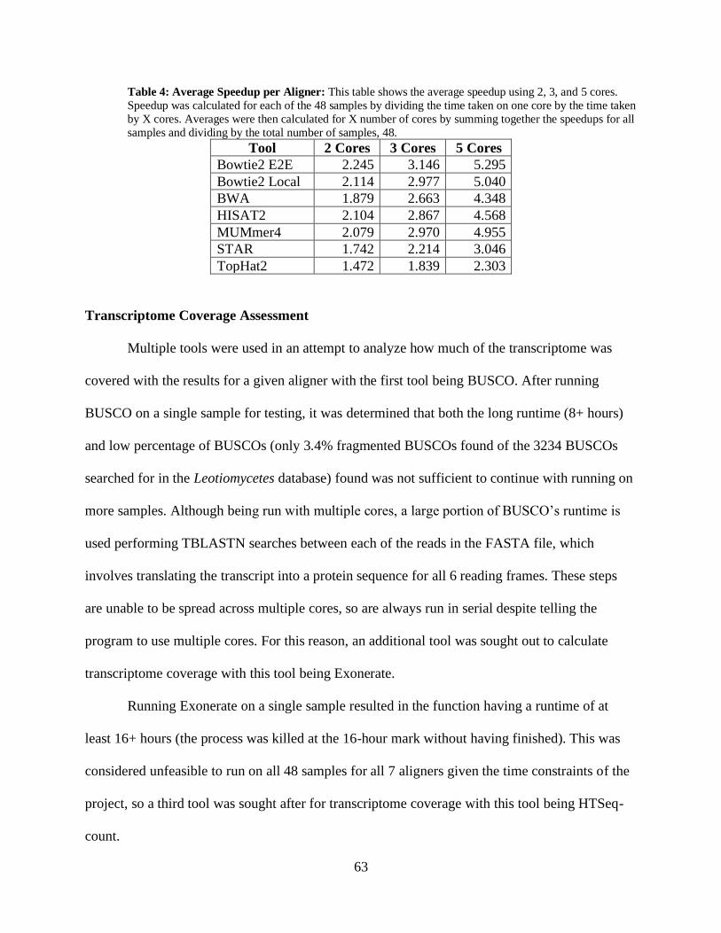
63

Table 4: Average Speedup per Aligner: This table shows the average speedup using 2, 3, and 5 cores.

Speedup was calculated for each of the 48 samples by dividing the time taken on one core by the time taken

by X cores. Averages were then calculated for X number of cores by summing together the speedups for all

samples and dividing by the total number of samples, 48.

Tool 2 Cores 3 Cores 5 Cores

Bowtie2 E2E 2.245 3.146 5.295

Bowtie2 Local 2.114 2.977 5.040

BWA 1.879 2.663 4.348

HISAT2 2.104 2.867 4.568

MUMmer4 2.079 2.970 4.955

STAR 1.742 2.214 3.046

TopHat2 1.472 1.839 2.303

Transcriptome Coverage Assessment

Multiple tools were used in an attempt to analyze how much of the transcriptome was

covered with the results for a given aligner with the first tool being BUSCO. After running

BUSCO on a single sample for testing, it was determined that both the long runtime (8+ hours)

and low percentage of BUSCOs (only 3.4% fragmented BUSCOs found of the 3234 BUSCOs

searched for in the Leotiomycetes database) found was not sufficient to continue with running on

more samples. Although being run with multiple cores, a large portion of BUSCO’s runtime is

used performing TBLASTN searches between each of the reads in the FASTA file, which

involves translating the transcript into a protein sequence for all 6 reading frames. These steps

are unable to be spread across multiple cores, so are always run in serial despite telling the

program to use multiple cores. For this reason, an additional tool was sought out to calculate

transcriptome coverage with this tool being Exonerate.

Running Exonerate on a single sample resulted in the function having a runtime of at

least 16+ hours (the process was killed at the 16-hour mark without having finished). This was

considered unfeasible to run on all 48 samples for all 7 aligners given the time constraints of the

project, so a third tool was sought after for transcriptome coverage with this tool being HTSeq-

count.

64

Running HTSeq-count on a single alignment file completed in under one minute but

reported no features found within the SAM file. Upon looking further into the code, it was found

that HTSeq-count does not perform any comparisons between the sequence content in the reads

from the alignment file, but instead counts the number of times that a given transcript’s name

(given by the feature file) appears within the SAM file. As the alignment files were aligned using

the reference genome and not the transcript file, the names present in the SAM file were those of

the contigs in the reference genome file. Therefore, the transcript names did not appear in the

alignment, which was the reason HTSeq-count reported all features to be missing. As the number

of transcripts found was not available from these results, yet another tool was used for

transcriptome coverage with this tool being BLAST+.

BLAST+ was run to align the combined and assembled reads of all 48 samples for a

given aligner (for example, all 48 sample’s aligned reads using BWA were combined into a

single FASTA file and assembled) as a database and the Cantu Lab’s E. necator transcriptome as

a query. Combining the alignment results of all 48 files was done with the hopes to remove any

potential bias of a particular sample not having a high enough expression of a gene (or not

containing the gene at all), due to the samples coming from various geographic climates. A low

expression for a given gene could result in the transcript either not being sequenced initially or

being removed during quality control. BLAST+ results reported which of the known E. necator

transcripts (given by the Cantu Lab’s file) were found within an aligner’s “database” of samples.

These alignment results were then analyzed for how complete the coverage of the full

transcriptome was at varying alignment length cutoffs (Figure 21). This analysis was able to

compare the aligners in multiple ways: 1) overall transcriptome coverage and 2) how well an

aligner was at generating transcripts of larger size (after assembling the reads of 48 “replicates”).

65

Overall, six of the seven aligners (all but TopHat2) were able to align > ~90% of the

transcriptome using alignments that were at least 100 bases long. Bowtie2 (95.6% in end-to-end

and 97.1% in local) and BWA (97.8%) had the three highest coverages and were almost able to

cover the full transcriptome at this cutoff. In contrast, TopHat2 had the lowest coverage using

this cutoff with only 74.1% transcripts found. Interestingly, both STAR and HISAT2 had slightly

higher coverage for alignment lengths > 1,000 bases than the other five aligners which all

converged into nearly the same values.

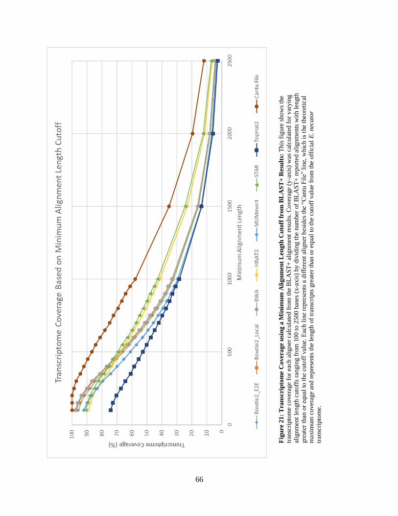
66

Fig

ure

21:

Tra

nsc

rip

tom

e C

overa

ge

usi

ng

a M

inim

um

Ali

gn

men

t L

en

gth

Cu

toff

fro

m B

LA

ST

+ R

esu

lts:

This

fig

ure

show

s th

e

tran

scri

pto

me

cover

age

for

each

ali

gn

er c

alcu

late

d f

rom

th

e B

LA

ST

+ a

lig

nm

ent

resu

lts.

Co

ver

age

(y-a

xis

) w

as c

alcu

late

d f

or

var

yin

g

alig

nm

ent

length

cuto

ffs

rangin

g f

rom

10

0 t

o 2

50

0 b

ases

(x-a

xis

) b

y d

ivid

ing

th

e n

um

ber

of

BL

AS

T+

rep

ort

ed a

lignm

ents

wit

h l

ength

gre

ater

th

an o

r eq

ual

to

th

e cu

toff

val

ue.

Eac

h l

ine

rep

rese

nts

a d

iffe

ren

t al

ign

er b

esid

es t

he

“Can

tu F

ile”

lin

e, w

hic

h i

s th

e th

eore

tica

l

max

imum

cover

age

and r

epre

sents

th

e le

ng

th o

f tr

ansc

ripts

gre

ater

than

or

equal

to t

he

cuto

ff v

alue

from

the

off

icia

l E

. nec

ato

r

tran

scri

pto

me.

67

Checking for Gene Bias

After analyzing the number of genes that were mapped by each aligner, the next step was

to examine those transcripts which were unmapped to determine if one aligner had difficulty

aligning a particular category of genes. To do this, genes from the Cantu transcriptome that were

not aligned by a certain aligner (did not have a hit from the BLAST+ analysis) were run through

EggNOG-mapper in order to annotate these unmapped genes. EggNOG-mapper reports

annotations from various databases, such as Kyoto Encyclopedia of Genes and Genomes and

Gene Ontology, but also includes annotations from Clusters of Orthologous Groups of proteins

(COG) (Tatusov et al., 2000), which categorizes genes based on their function into 26 distinct

categories (Table 5). To check for any bias in unmapped transcripts, the resulting COG

categories were examined for overrepresentation within a given aligner. Overall, all aligners

tested had similar distributions between COG categories with categories ‘L’ (“Replication,

Recombination, and Repair”) and ‘S’ (“Function Unknown”) being overrepresented in each. The

lowest number of unmapped reads was 106 from BWA with ~20% of these genes belonging to

the “Replication, Recombination, and Repair” category and ~12% belonging to “Function

Unknown”. The highest number of unmapped reads belonged to TopHat2 with a total number of

1,570 unmapped genes resulting in ~12% belonging to “Replication, Recombination, and

Repair” and ~29% belonging to “Function Unknown”. Interestingly, as the number of unmapped

reads increased between aligners, the percentage of genes belonging to “Replication,

Recombination, and Repair” steadily decreased and the percentage of genes belonging to

“Function Unknown” steadily increased (shown in Figure 22A-D; other aligners in

Supplementary A1-A3). From these results, it was determined that no aligner had more trouble

than another with aligning a particular category of genes as all aligners had the same categories

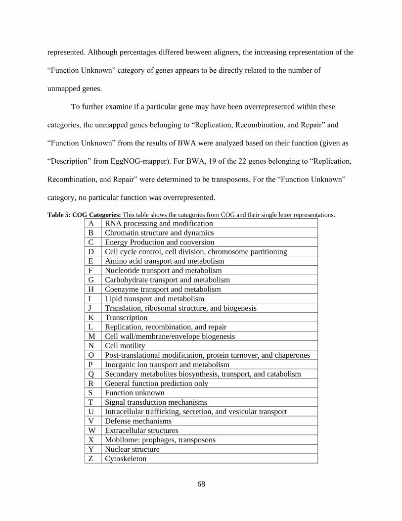
68

represented. Although percentages differed between aligners, the increasing representation of the

“Function Unknown” category of genes appears to be directly related to the number of

unmapped genes.

To further examine if a particular gene may have been overrepresented within these

categories, the unmapped genes belonging to “Replication, Recombination, and Repair” and

“Function Unknown” from the results of BWA were analyzed based on their function (given as

“Description” from EggNOG-mapper). For BWA, 19 of the 22 genes belonging to “Replication,

Recombination, and Repair” were determined to be transposons. For the “Function Unknown”

category, no particular function was overrepresented.

Table 5: COG Categories: This table shows the categories from COG and their single letter representations.

A RNA processing and modification

B Chromatin structure and dynamics

C Energy Production and conversion

D Cell cycle control, cell division, chromosome partitioning

E Amino acid transport and metabolism

F Nucleotide transport and metabolism

G Carbohydrate transport and metabolism

H Coenzyme transport and metabolism

I Lipid transport and metabolism

J Translation, ribosomal structure, and biogenesis

K Transcription

L Replication, recombination, and repair

M Cell wall/membrane/envelope biogenesis

N Cell motility

O Post-translational modification, protein turnover, and chaperones

P Inorganic ion transport and metabolism

Q Secondary metabolites biosynthesis, transport, and catabolism

R General function prediction only

S Function unknown

T Signal transduction mechanisms

U Intracellular trafficking, secretion, and vesicular transport

V Defense mechanisms

W Extracellular structures

X Mobilome: prophages, transposons

Y Nuclear structure

Z Cytoskeleton

69

Fig

ure

22:

CO

G C

ate

gory D

istr

ibu

tio

ns

for

Un

ma

pp

ed

Tra

nsc

rip

ts:

Th

is f

igu

re s

ho

ws

the

CO

G c

ateg

ory

dis

trib

uti

ons

that

are

repre

sente

d b

y t

he

unm

apped

tra

nsc

ripts

fo

r fo

ur

rep

rese

nta

tive

alig

ner

s. F

igu

re A

is

for

BW

A, F

igure

B i

s fo

r B

ow

tie

in e

nd

-

to-e

nd m

ode,

Fig

ure

C i

s fo

r S

TA

R, an

d F

igu

re D

is

for

To

pH

at2. T

he

num

ber

of

un

map

ped

tra

nsc

ripts

is

list

ed a

s th

e val

ue

of

‘n’

in e

ach

fig

ure

’s t

itle

an

d t

he

val

ue

incr

ease

s fr

om

Fig

ure

A (

min

val

ue)

to

D (

max

val

ue)

. T

he

x-a

xis

lis

ts t

he

sin

gle

let

ter

corr

espondin

g t

o e

ach C

OG

cat

ego

ry (

A-Z

) al

on

g w

ith “

Unca

t” (

tran

scri

pts

th

at h

ad E

gg

NO

G-m

apper

res

ult

s but

no C

OG

cate

gory

) an

d “

No R

esult

s” (

tran

scri

pts

that

did

not

hav

e an

y r

esult

s fr

om

Eg

gN

OG

-map

per

). T

he

y-a

xis

rep

rese

nts

the

per

centa

ge

of

unm

apped

tra

nsc

ripts

bel

ong

ing t

o e

ach

cat

ego

ry.

70

Discussion

The field of bioinformatics is constantly flooded with new tools claiming to be the best at

what they do. Often trying to search for a tool to do the required job yields more questions than

answers by giving the researcher too many options to choose from. The aim of this project was to

ease that burden in terms of searching for which genome aligner performs the best. By using a

consistent dataset and running the aligners on their default settings, performance for each aligner

was determined by the algorithms built into the tools themselves. If the algorithms were

independent of overall performance, then all genome aligners should generate the same results

given the same dataset. As this study has shown, this was not the case as aligners such as

TopHat2 struggled to keep up with many of the other aligners like STAR and BWA. Aligners

differed in the number of reads that were successfully mapped, overall runtimes, efficiency of

using multiple cores for parallel computing, and transcriptome coverage completeness.

Using Default Settings

There are two major reasons for why default settings were used in this project. The first

reason being that there is an assumption being made that the developers for each aligner

thoroughly tested there product and assigned default values for which the aligner performs best

on most datasets. Another reason involves who is actually going to be using these types of tools

out in the field. A researcher who is using a genome aligner is most likely not familiar enough

with the function of each of the variables and how much of an impact changing one of these

values will have on the output. Further, a majority of the time when using a tool such as a

genome aligner the tool will always first be run using its default settings. If the results are

sufficient enough, the researcher will move on with their work and have only ever run the tool

with its default settings. If more work needs to be done at the alignment step, then extra care is

71

taken to change variables as needed to get the intended results. Since running on the default

settings is often used as an initial test of an aligner’s overall performance, it is important for the

tool to perform well using these settings.

Correlations Between Alignment Rate & Runtime per Read

One interesting finding during this analysis was the correlation between alignment rates

and runtime per read that was discovered in a majority of the aligners. The initial hypothesis was

that normalizing the runtimes by the number of reads in each sample would remove any

correlation. Theoretically, a sample with 1,000 reads should take roughly 10x’s longer to process

than a sample with 100 reads. By removing this variable, one would assume that a sample that

had a longer runtime would not necessarily result in a higher alignment rate and therefore no

correlation should be found between alignment rate and runtime as seen in aligners like HISAT2

and TopHat2. However, most of the aligners tested resulted in a positive correlation between

these two variables. Overall, Bowtie2 (in local and end-to-end mode) had a strong positive

correlation and BWA and MUMmer4 had slightly positive correlations. The reason for a positive

correlation between these two variables may simply come down to how an aligner stores an

alignment. Prior to reporting all alignments for a given sample, an aligner must create a data

structure to store all current alignments. Most often, an aligner has some order as to where an

alignment is placed within the structure and may not simply attach the next alignment to the end

of the queue as would occur in an array. As the data structure grows more complex by adding

more alignments, it gets computationally more intense to traverse and add an additional

alignment to its designated place in the structure. In a simple example, if one was to be given a

random number and told to place that number in its correct position, it is much easier (and faster)

to find this number’s correct position in a list of 10 numbers than a list of 100 numbers.

72

Assuming that these lists of numbers are now the data structure filled with already aligned reads,

finding the correct location for the next aligned read becomes more difficult and therefore

requires more time as the alignment rate increases.

Additionally, STAR resulted in a negative correlation between runtime and alignment

rate. This means that the longer it took to run, the lower the number of successfully mapped

reads would be and ultimately letting the aligner run for a long period of time would only result

in worse alignment rates. Although this seems inexplicable, if this correlation was defined in

terms of the percentage of unmapped reads, a better solution presents itself. A sample with a low

alignment rate inherently has a large percentage of unmapped reads. Relating this back to the

initial negative correlation yields the idea that a large percentage of unmapped reads results in a

longer runtime, meaning that STAR may spend longer time than other aligners at attempting to

align unmappable reads. Although this seems like a poor quality for an aligner to have, it may

give STAR an advantage when trying to align transcripts that are often misaligned by other

aligners either due to the reads being of low quality or highly variable such as having a higher

SNP rate than others. This idea is further reinforced by the fact that STAR accounts for higher

variability by allowing for a greater number of mismatches in resulting alignments than other

aligners. Whereas other aligners negatively weight a mismatch when calculating an alignments

overall score (see the “Mismatch” column in Table 1), STAR allows for a maximum of 10

mismatched bases by default for a given alignment. In contrast, TopHat2 only allows for a

maximum of 2 mismatches before terminating an alignment. This higher mismatch tolerance

would allow for STAR to align more highly variable transcripts, but ultimately hinder its runtime

when aligning reads in a less variable specie.

73

Explanation of Speedup Curves

When examining speedup curves, a tool is always judged based on how much the curve

itself differs from the line y = x. This is because a linear line represents a tool running X times

faster on X number of cores and therefore has an ideal linear speedup. Although ideal, linear

speedup is often rare as simply adding to the number of cores being used does not guarantee that

a process will run faster. Instead, the code itself must be structured accordingly to accommodate

using more cores. Often there are large portions of code which can only be run in serial (on 1

corre). This results in a tool beginning with using only 1 core, then a point is reached in the

process where work can be divided among multiple cores, followed by the tool normally

finishing in serial. Therefore, speedup depends mainly on the runtime and complexity of these

portions of code that must be run in serial. If the serial portions are time consuming as they

appear to be in TopHat2 and STAR, using a large number of cores will not necessarily result in

faster times, resulting in a logarithmic curve. If the code is well-structured and ready for

parallelization, such as Bowtie2 in local mode, BWA, HISAT2, and MUMmer4, an ideal linear

speedup is achieved.

In other cases, such as Bowtie2 in end-to-end mode, super-linear speedup is found which

results in a tool performing > X times faster on X cores. Super-linear speedup is most often

achieved due to parallel computing taking advantage of an increased cache of memory outside of

the constantly available random access memory (RAM) (Ristov et al., 2016). For example, say

that a computer has 5 available processing cores that can each hold 1 MB of data resulting in a

total cache of 5 MB. Next, assume that the data being used requires 4 MB to run to completion.

If only one core was being used, the machine only has access to 1 MB of the data at a time. The

other 3 MB of data are stored in RAM. When the first 1 MB of data has been processed, the next

74

1 MB must be transferred between RAM and the central processing unit (CPU). If all 5 cores

were being utilized, all 5 MB of data could be processed at once without the use of RAM and

therefore the additional step of transferring data between RAM and CPU would not be required

(data must still be transferred between CPU and memory cache but RAM is not required). This

increase in available cached memory by using multiple cores is often the most logical reason for

super-linear speedup.

Sample Outliers

Across all aligners tested, 46 of the 48 samples appeared to cluster well together in terms

of their runtime and alignment rate. Interestingly, the same two samples, A06 and D11, were

listed as outliers for nearly every aligner with most aligners finding lower alignment rates for

these samples compared to the others. As the 48 samples of E. necator were all from

geographically distinct locations, one could assume that these two samples were from the same

region and perhaps genetically distinct from the reference genome used. Although both samples

came from the southern region of the United States, sample A06 came from the more central

United States in Purdy, Missouri whereas sample D11 came from the eastern United States in

Mocksville, North Carolina (see Supplementary S4). Additionally, these samples were not the

only samples used in this project from these respective areas. There were 2 other samples from

the state of Missouri and 7 other samples from North Carolina. It was also suspected that these

samples may have had two of the smallest number of reads after quality control and were

therefore at a disadvantage initially prior to alignment. However, both samples had nearly the

same number of reads (A06 had 741,883 and D11 had 737,552) with these counts being nearly

equivalent to the average read count of 741,219. Aside from being technical outliers, there

75

appears to be no biological reason why these samples continuously had lower alignment rates

than the others.

Transposon Bias

After checking for a bias in the type of genes which were unable to be aligned, it was

discovered that a large portion of these genes were transposons. Although it may seem that an

aligner’s struggle with aligning transposons comes from the gene’s function, it most likely has to

do with overall sequence of the gene and has little to do with function if at all. Transposable

elements have caused trouble for researchers trying to align them in the past due to their

sequences being made up of large sections of repeatable elements. Aligners often struggle with

aligning repeatable sequences as these reads often are aligned to multiple locations in the

genome. Some aligners will weight an alignment negatively if a read is assigned to multiple

locations and therefore may not report the resulting alignment to the user. Other aligners, such as

most of the aligners tested in this project, report a large number of potential alignments and will

list separately in their output that “X number of reads were aligned to >1 location”. However,

even listing multiple alignments does not seem to be enough to aid in the alignment of

transposons. Teissandier et al. discovered that using paired end data (single end was used in this

project) results in a better mapping rate of transposons as well as having aligners report multiple

hits for every read aligned (Teissandier et al., 2019). In other words, it is not uncommon for a

study such as this to identify a large number of unmapped transposons.

“Best” Aligner

To determine which aligner performed the “best”, a few clarifications must first be made.

First, aligners behave differently when using different datasets. This could be due to biological

differences such as GC content and proportion of repeated elements, which was discussed

76

previously as being troublesome for aligners. Another difference guaranteed to make an impact

is a more technical issue with the overall quality of the dataset being used. The dataset used in

this project had very poor quality and attempts to clean up the reads saw roughly 80% of reads

removed. It is possible for a much cleaner dataset having much different results then the ones

portrayed here. Therefore, the results of this project can be seen as which aligner performed best

on this dataset for E. necator. Second, with fine tuning of the parameters, it is possible for other

aligners to outperform one another. This project worked under the assumption that the creators of

each tool allowed for the default settings to result in the best quality results for an aligner.

Additionally, RNA-seq based aligners, such as HISAT2, STAR, and TopHat2, all were run

without the use of an annotated transcriptome. It is speculated that running these aligners with an

annotation file results in higher mapping rates, however, to keep all aligners on the same level, it

was decided against for this project.

Deciding on which aligner performed the best came down to which tool achieved the best

balance of the two major categories: speed and accuracy. Analyzing the results as is made

deciding on which aligner was the “best” difficult. In contrast, the worst aligner on this dataset

was TopHat2, which had the longest runtimes and the lowest alignment rate by a large margin.

To better illustrate the major differences between all aligners tested, a figure was generated

(which excluded TopHat2 to show a greater difference between individual aligners) to directly

compare the average runtime per read with the average alignment rate for a given aligner (Figure

23). The first conclusion drawn from this figure was that Bowtie2 in local mode and BWA had a

near tie for the highest alignment rate, however BWA’s lesser runtime results in the tool being

preferable. Similar reasoning was applied to determining STAR being a better tool to use over

MUMmer4 and HISAT2 over Bowtie2 in end-to-end mode. When comparing BWA to STAR,

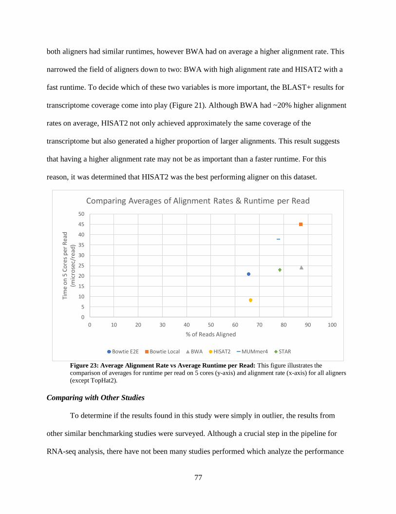
77

both aligners had similar runtimes, however BWA had on average a higher alignment rate. This

narrowed the field of aligners down to two: BWA with high alignment rate and HISAT2 with a

fast runtime. To decide which of these two variables is more important, the BLAST+ results for

transcriptome coverage come into play (Figure 21). Although BWA had ~20% higher alignment

rates on average, HISAT2 not only achieved approximately the same coverage of the

transcriptome but also generated a higher proportion of larger alignments. This result suggests

that having a higher alignment rate may not be as important than a faster runtime. For this

reason, it was determined that HISAT2 was the best performing aligner on this dataset.

Figure 23: Average Alignment Rate vs Average Runtime per Read: This figure illustrates the

comparison of averages for runtime per read on 5 cores (y-axis) and alignment rate (x-axis) for all aligners

(except TopHat2).

Comparing with Other Studies

To determine if the results found in this study were simply in outlier, the results from

other similar benchmarking studies were surveyed. Although a crucial step in the pipeline for

RNA-seq analysis, there have not been many studies performed which analyze the performance

0

5

10

15

20

25

30

35

40

45

50

0 10 20 30 40 50 60 70 80 90 100

Tim

e o

n 5

Co

res

per

Rea

d(m

icro

sec/

read

)

% of Reads Aligned

Comparing Averages of Alignment Rates & Runtime per Read

Bowtie E2E Bowtie Local BWA HISAT2 MUMmer4 STAR

78

of the aligners themselves as many studies choose to compare tools used downstream when

performing differential expression. Of the few studies found, no particular study used the same

exact set of aligners, however most of them contained at least two of the tools which allowed for

some comparative conclusions to the project performed here. For example, many of the studies

found that STAR almost always outperformed TopHat2 in terms of higher alignment rates as

well as reporting less mismatches in the overall alignments (Engström et al., 2013; Teng et al.,

2016). Additionally, TopHat2 was found to perform better (higher alignment rates) when using

an annotation file (Engström et al., 2013). Similar to this project, one study found that HISAT2

outperformed both STAR and BWA in regards to runtime by a factor of 1.7 and 3.4 respectively

(Lachmann et al., 2020). This same study also found that although BWA recorded the highest

gene counts (similar to the higher alignment rates reported here) it was determined during

differential expression analysis that BWA recorded the lowest number of enriched biological

terms (Lachmann et al., 2020). This finding confirms the conclusion for the project outlined in

this paper that having a high alignment rate does not necessarily guarantee better results as found

by the similar transcriptome coverages for all aligners.

Future Work

To officially determine which aligner is the best, a wide variety of datasets must be used

consisting of datasets for various organisms, datasets ranging from low to high quality, etc.

Projects similar to this one could be performed by comparing an aligners ability to process data

of different quality and from other organisms to determine if the results found for aligning

average quality reads for E. necator (as performed here) are comparable. It is possible that an

aligner such as TopHat2 only performs well with extremely high-quality data, which would

drastically increase its alignment rate but also makes the tool impractical to use as extremely

79

high-quality data is expensive to produce. Also, STAR, TopHat2, and HISAT2 were

theoretically run at a disadvantage to keep them on the same level as the other aligners tested that

were unable to accept annotation files. All three of these aligners are specifically designed to

align RNA-seq reads to a reference genome with added help from an annotated transcriptome for

the same species. Assuming that running these aligners with a transcriptome attached would

increase alignment rates, it may result in an aligner such as STAR surpassing BWA in terms of

average alignment rate. Additionally, it may increase HISAT2’s alignment rate, further

separating it from the other aligners. Another area for future work comes from the fact that tools

for bioinformatics are constantly being updated, so it is inevitable that an aligner such as

HISAT3 or STAR2 should eventually release with the authors claiming that this new

tool/version is the “best” aligner available. Adding the results from that new aligner to a project

such as this would truly determine how much better the aligner is against its competition.

80

Works Cited

1. aechchiki, “gffread: GFaSeqGet errors on coordinate overhang”, Stack Exchange, 2018

[https://bioinformatics.stackexchange.com/questions/3651/gffread-gfaseqget-errors-on-

coordinate-overhang]

2. Altschul SF, Gish W, Miller W, Myers EW, Lipman DJ, “Basic Local Alignment Search

Tool”, J Mol Biol, 1990, vol. 215, no. 3 (pg. 403-10)

3. Anders S, Pyl TP, Huber W, “HTSeq - A Python Framework to Work with High-

Throughput Sequencing Data”, bioRxiv, 2014

4. Andrews S, FastQC (v0.11.7), 2018

[https://www.bioinformatics.babraham.ac.uk/projects/fastqc/]

5. Cadle-Davidson L, Wakefield L, Seem RC, Gadoury DM, “Specific Isolation of RNA

from the Grape Powdery Mildew Pathogen Erysiphe necator, an Epiphytic, Obligate

Parasite”, Journal of Phytopathology, 2009, vol. 158, no. 1 (pg. 69-71)

6. Camacho C, Coulouris G, Avagyan V, Ma N, Papadopoulos J, Bealer K, Madden TL,

“BLAST+: Architecture and Applications”, BMC Bioinformatics, 2009, vol. 10, no. 421

7. Chhangawala S, Rudy G, Mason CE, Rosenfeld JA, “The Impact of Read Length on

Quantification of Differentially Expressed Genes and Splice Junction Detection”,

Genome Biology, 2015, vol. 16, no. 131

8. Delcher AL, Kasif S, Fleischmann RD, Peterson J, White O, Salzberg SL, “Alignment of

Whole Genomes”, Nucleic Acids Research, 1999, vol. 27, no. 11 (pg. 2369-76)

9. Delcher AL, Phillippy A, Carlton J, Salzberg SL, “Fast Algorithms for Large-Scale

Genome Alignment and Comparison”, Nucleic Acids Research, 2002, vol. 30, no. 11 (pg.

2478-83)

10. Dobin A, Davis CA, Schlesinger F, Drenkow J, Zaleski C, Jha S, Batut P, Chaisson M,

Gingeras TR, “STAR: Ultrafast Universal RNA-seq Aligner”, Bioinformatics, 2013, vol.

29, no. 1, (pg. 15-21)

11. Engström PG, Steijger T, Sipos B, Grant GR, Kahles A, The RGASP Consortium, Rätsch

G, Goldman N, Hubbard TJ, Harrow J, Guigó R, Bertone P, “Systemic Evaluation of

Spliced Alignment Programs for RNA-seq Data”, Nature Methods, 2013, vol. 10 (pg.

1185-91)

12. Erysiphe necator Annotation GFF: Downloaded February 2020 from

https://cantulab.github.io/e-necator.c-strain.gff.gz

13. Erysiphe necator Peptides: Downloaded February 2020 from

https://cantulab.github.io/E.necator.proteins.NCBI.6533.fasta.gz

14. Erysiphe necator Reference Genome: Downloaded November 2019 from

https://cantulab.github.io/e-necator.scaffolds.c.NCBI.fasta.gz

15. Erysiphe necator Transcripts: Downloaded March 2020 from

https://cantulab.github.io/E.necator.transcripts.NCBI.6533.fasta.gz

16. Ferragina P, Manzini G, “Opportunistic Data Structures with Applications”, Proceedings

41st Annual Symposium on Foundations of Computer Science, 2000 (pg. 390-8)

17. Hannon GJ, FASTX-Toolkit (v0.0.13), 2010 [http://hannonlab.cshl.edu/fastx_toolkit/]

18. Huerta-Cepas J, Forslund K, Coelho LP, Szklarczyk D, Jensen LJ, von Mering C, Bork P,

“Fast Genome-Wide Functional Annotation through Orthology Assignment by eggNOG-

Mapper”, Molecular Biology and Evolution, 2017, vol. 34, no. 8 (pg. 2115-22)

81

19. Jones L, Riaz S, Morales-Cruz A, Amrine KCH, McGuire B, Gubler MA, Cantu D,

“Adaptive Genomic Structural Variation in the Grape Powdery Mildew Pathogen,

Erysiphe necator”, BMC Genomics, 2014, vol. 15, no. 1081

20. Lachmann A, Clarke DJB, Torre D, Xie Z, Ma’ayan A, “Interoperable RNA-Seq

Analysis in the Cloud”, Biochimica et Biophysica Acta (BBA) - Gene Regulatory

Mechanisms, 2020, vol. 1863, no. 6

21. Langmead B, Salzberg SL, “Fast Gapped-Read Alignment with Bowtie 2”, Nature

Methods, 2012, vol. 9 (pg. 357-59)

22. Langmead B, Trapnell C, Pop M, Salzberg SL, “Ultrafast and Memory-Efficient

Alignment of Short DNA Sequences to the Human Genome”, Genome Biology, 2009,

vol. 10, no. R25

23. Li H, “Aligning Sequence Reads, Clone Sequences and Assembly Contigs with BWA-

MEM”, arXiv:1303.3997v2, 2013

24. Li H, Durbin R, “Fast and Accurate Short Read Alignment with Burrows-Wheeler

Transform”, Bioinformatics, 2009, vol. 25, no. 14 (pg. 1754-60)

25. Li H, Homer N, “A Survey of Sequence Alignment Algorithms for Next-Generation

Sequencing”, Briefings in Bioinformatics, 2010, vol. 11, no. 5 (pg. 473-83)

26. Kim D, Langmead B, Salzberg SL, “HISAT: A Fast Spliced Aligner with Low Memory

Requirements” Nature Methods, 2015, vol. 12, no. 4

27. Kim D, Paggi JM, Park C, Bennett C, Salzberg SL, “Graph-based Genome Alignment

and Genotyping with HISAT2 and HISAT-genotype”, Nature Biotechnology, 2019, vol.

37 (pg. 907-15)

28. Kim D, Pertea G, Trapnell C, Pimentel H, Kelley R, Salzberg SL, “TopHat2: Accurate

Alignment of Transcriptomes in the Presence of Insertions, Deletions and Gene Fusions”,

Genome Biology, 2013, vol. 14, no. R36

29. Kurtz S, Phillippy A, Delcher AL, Smoot M, Shumway M, Antonescu C, Salzberg SL,

“Versatile and Open Software for Comparing Large Genomes”, Genome Biol, 2004, vol.

5, no. 2 (pg. R12)

30. Marçais G, Delcher AL, Phillippy AM, Coston R, Salzberg SL, Zimin A, “MUMmer4: A

Fast and Versatile Genome Alignment System”, PLOS Computational Biology, 2018,

vol. 14, no. 1

31. Marshall J, Bonfield J, Danecek P, “Sequence Alignment/Map Format Speciation”, 2009

[https://samtools.github.io/hts-specs/SAMv1.pdf]

32. Ristov S, Prodan R, Gusev M, Skala K, “Superlinear Speedup in HPC Systems: Why and

When?”, Proceedings of the Federated Conference on Computer Science and

Information Systems, 2016, vol. 8 (pg. 889-98)

33. Simão FA, Waterhouse RM, Ioannidis P, Kriventseva EV, Zdobnov EM, “BUSCO:

Assessing Genome Assembly and Annotation Completeness with Single-Copy

Orthologs”, Bioinformatics, 2015, vol. 31, no. 19 (pg. 3210-12)

34. Slater GSC, Birney E, “Automated Generation of Heuristics for Biological Sequence

Comparison”, BMC Bioinformatics, 2005, vol. 6, no. 31

35. Tatusov RL, Galperin MY, Natale DA, Koonin EV, “The COG Database: A Tool for

Genome-Scale Analysis of Protein Functions and Evolution”, Nucleic Acids Research,

2000, vol. 28, no. 1 (pg. 33-36)

82

36. Teissandier A, Servant N, Barillot E, Bourc’his D, “Tools and Best Practices for

Retrotransposon Analysis using High-Throughput Sequencing Data”, Mobile DNA, 2019,

vol. 10, no. 52

37. Teng M, Love MI, Davis CA, Djebali S, Dobin A, Graveley BR, Li S, Mason CE, Olson

S, Pervouchine D, Sloan CA, Wei X, Zhan L, Irizarry RA, “A Benchmark for RNA-seq

Quantification Pipelines”, Genome Biology, 2016, vol. 17, no. 74

38. Trapnell C, Pachter L, Salzberg SL, “TopHat: Discovering Splice Junctions with RNA-

Seq”, Bioinformatics, 2009, vol. 25, no. 9 (pg. 1105-11)

39. Trapnell C, Williams BA, Pertea G, Mortazavi A, Kwan G, van Baren MJ, Salzberg SL,

Wold BJ, Pachter L, “Transcript Assembly and Quantification by RNA-Seq Reveals

Unannotated Transcripts and Isoform Switching During Cell Differentiation”, Nature

Biotechnology, 2010, vol. 28 (pg. 511-15)

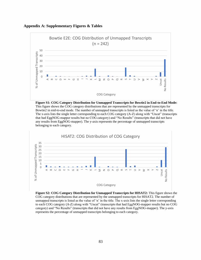
83

Appendix A: Supplementary Figures & Tables

Figure S1: COG Category Distribution for Unmapped Transcripts for Bowtie2 in End-to-End Mode:

This figure shows the COG category distributions that are represented by the unmapped transcripts for

Bowtie2 in end-to-end mode. The number of unmapped transcripts is listed as the value of ‘n’ in the title.

The x-axis lists the single letter corresponding to each COG category (A-Z) along with “Uncat” (transcripts

that had EggNOG-mapper results but no COG category) and “No Results” (transcripts that did not have

any results from EggNOG-mapper). The y-axis represents the percentage of unmapped transcripts

belonging to each category.

Figure S2: COG Category Distribution for Unmapped Transcripts for HISAT2: This figure shows the

COG category distributions that are represented by the unmapped transcripts for HISAT2. The number of

unmapped transcripts is listed as the value of ‘n’ in the title. The x-axis lists the single letter corresponding

to each COG category (A-Z) along with “Uncat” (transcripts that had EggNOG-mapper results but no COG

category) and “No Results” (transcripts that did not have any results from EggNOG-mapper). The y-axis

represents the percentage of unmapped transcripts belonging to each category.

0

10

20

30

40

50A B C D E F G H I J K L M N O P Q R S T U V W X Y Z

Un

cat

No

Res

ult

s

% o

f U

nm

app

ed T

ran

scri

pts

COG Category

Bowtie E2E: COG Distribution of Unmapped Transcripts(n = 242)

05

101520253035

A B C D E F G H I J K L M N O P Q R S T U V W X Y Z

Un

cat

No

Res

ult

s

% o

f U

nm

app

ed T

ran

scri

pts

COG Category

HISAT2: COG Distribution of COG Category

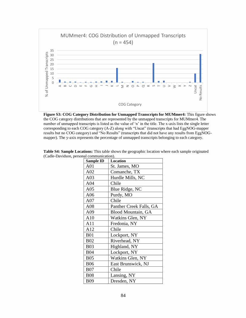
84

Figure S3: COG Category Distribution for Unmapped Transcripts for MUMmer4: This figure shows

the COG category distributions that are represented by the unmapped transcripts for MUMmer4. The

number of unmapped transcripts is listed as the value of ‘n’ in the title. The x-axis lists the single letter

corresponding to each COG category (A-Z) along with “Uncat” (transcripts that had EggNOG-mapper

results but no COG category) and “No Results” (transcripts that did not have any results from EggNOG-

mapper). The y-axis represents the percentage of unmapped transcripts belonging to each category.

Table S4: Sample Locations: This table shows the geographic location where each sample originated

(Cadle-Davidson, personal communication).

Sample ID Location

A01 St. James, MO

A02 Comanche, TX

A03 Hurdle Mills, NC

A04 Chile

A05 Blue Ridge, NC

A06 Purdy, MO

A07 Chile

A08 Panther Creek Falls, GA

A09 Blood Mountain, GA

A10 Watkins Glen, NY

A11 Fredonia, NY

A12 Chile

B01 Lockport, NY

B02 Riverhead, NY

B03 Highland, NY

B04 Lockport, NY

B05 Watkins Glen, NY

B06 East Brunswick, NJ

B07 Chile

B08 Lansing, NY

B09 Dresden, NY

05

10

15

20

2530

35

A B C D E F G H I J K L M N O P Q R S T U V W X Y Z

Un

cat

No

Res

ult

s

% o

f U

nm

app

ed T

ran

scri

pts

COG Category

MUMmer4: COG Distribution of Unmapped Transcripts(n = 454)

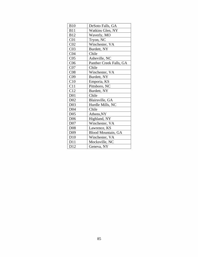
85

B10 DeSoto Falls, GA

B11 Watkins Glen, NY

B12 Waverly, MO

C01 Tryon, NC

C02 Winchester, VA

C03 Burdett, NY

C04 Chile

C05 Asheville, NC

C06 Panther Creek Falls, GA

C07 Chile

C08 Winchester, VA

C09 Burdett, NY

C10 Emporia, KS

C11 Pittsboro, NC

C12 Burdett, NY

D01 Chile

D02 Blairsville, GA

D03 Hurdle Mills, NC

D04 Chile

D05 Athens,NY

D06 Highland, NY

D07 Winchester, VA

D08 Lawrence, KS

D09 Blood Mountain, GA

D10 Winchester, VA

D11 Mocksville, NC

D12 Geneva, NY

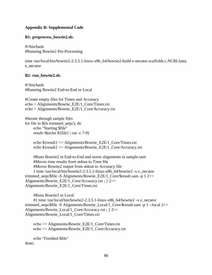
86

Appendix B: Supplemental Code

B1: preprocess_bowtie2.sh:

#!/bin/bash

#Running Bowtie2 Pre-Processing

time /usr/local/bin/bowtie2-2.3.5.1-linux-x86_64/bowtie2-build e-necator.scaffolds.c.NCBI.fasta

e_necator

B2: run_bowtie2.sh:

#!/bin/bash

#Running Bowtie2 End-to-End or Local

#Create empty files for Times and Accuracy

echo > Alignments/Bowtie_E2E/1_Core/Times.txt

echo > Alignments/Bowtie_E2E/1_Core/Accuracy.txt

#Iterate through sample files

for file in $(ls trimmed_seqs/); do

echo "Starting $file"

result=$(echo ${file} | cut -c 7-9)

echo ${result} >> Alignments/Bowtie_E2E/1_Core/Times.txt

echo ${result} >> Alignments/Bowtie_E2E/1_Core/Accuracy.txt

#Runs Bowtie2 in End-to-End and stores alignments in sample.sam

#Moves time results from stdout to Time file

#Moves Bowtie2 output from stdout to Accuracy file

{ time /usr/local/bin/bowtie2-2.3.5.1-linux-x86_64/bowtie2 -x e_necator

trimmed_seqs/$file -S Alignments/Bowtie_E2E/1_Core/$result.sam -p 1 2>>

Alignments/Bowtie_E2E/1_Core/Accuracy.txt ; } 2>>

Alignments/Bowtie_E2E/1_Core/Times.txt

#Runs Bowtie2 in Local

#{ time /usr/local/bin/bowtie2-2.3.5.1-linux-x86_64/bowtie2 -x e_necator

trimmed_seqs/$file -S Alignments/Bowtie_Local/1_Core/$result.sam -p 1 --local 2>>

Alignments/Bowtie_Local/1_Core/Accuracy.txt ; } 2>>

Alignments/Bowtie_Local/1_Core/Times.txt

echo >> Alignments/Bowtie_E2E/1_Core/Times.txt

echo >> Alignments/Bowtie_E2E/1_Core/Accuracy.txt

echo "Finished $file"

done;

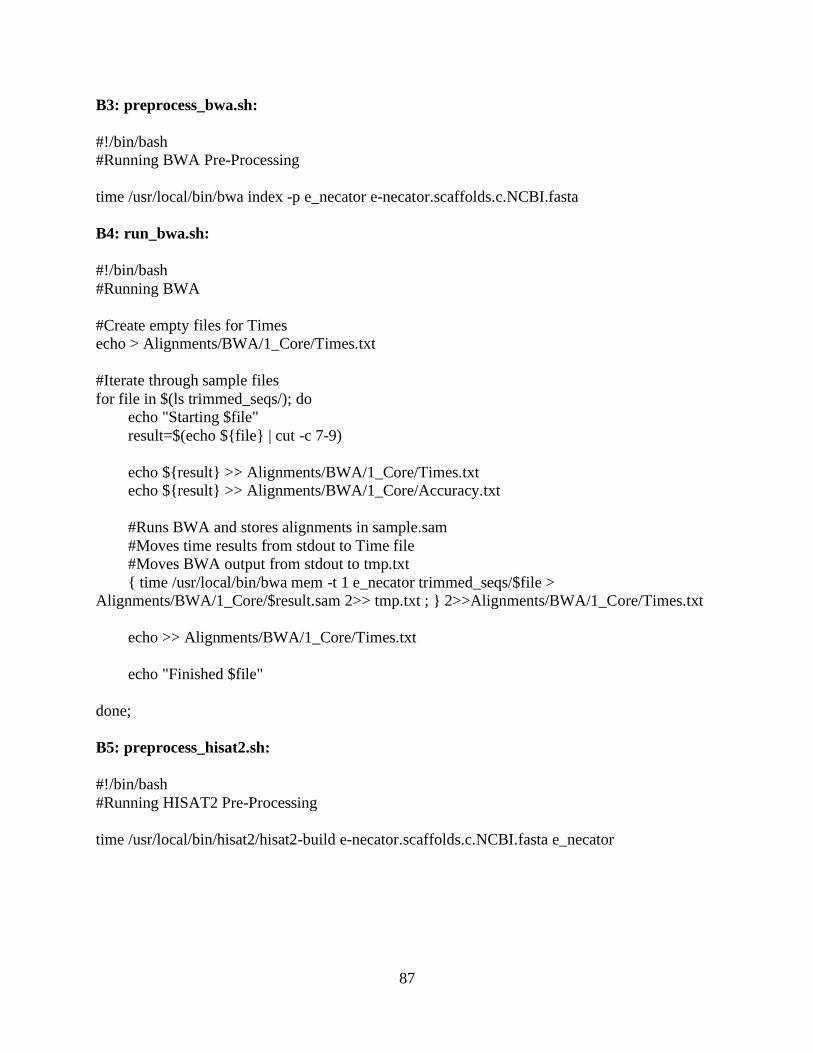
87

B3: preprocess_bwa.sh:

#!/bin/bash

#Running BWA Pre-Processing

time /usr/local/bin/bwa index -p e_necator e-necator.scaffolds.c.NCBI.fasta

B4: run_bwa.sh:

#!/bin/bash

#Running BWA

#Create empty files for Times

echo > Alignments/BWA/1_Core/Times.txt

#Iterate through sample files

for file in $(ls trimmed_seqs/); do

echo "Starting $file"

result=$(echo ${file} | cut -c 7-9)

echo ${result} >> Alignments/BWA/1_Core/Times.txt

echo ${result} >> Alignments/BWA/1_Core/Accuracy.txt

#Runs BWA and stores alignments in sample.sam

#Moves time results from stdout to Time file

#Moves BWA output from stdout to tmp.txt

{ time /usr/local/bin/bwa mem -t 1 e_necator trimmed_seqs/$file >

Alignments/BWA/1_Core/$result.sam 2>> tmp.txt ; } 2>>Alignments/BWA/1_Core/Times.txt

echo >> Alignments/BWA/1_Core/Times.txt

echo "Finished $file"

done;

B5: preprocess_hisat2.sh:

#!/bin/bash

#Running HISAT2 Pre-Processing

time /usr/local/bin/hisat2/hisat2-build e-necator.scaffolds.c.NCBI.fasta e_necator

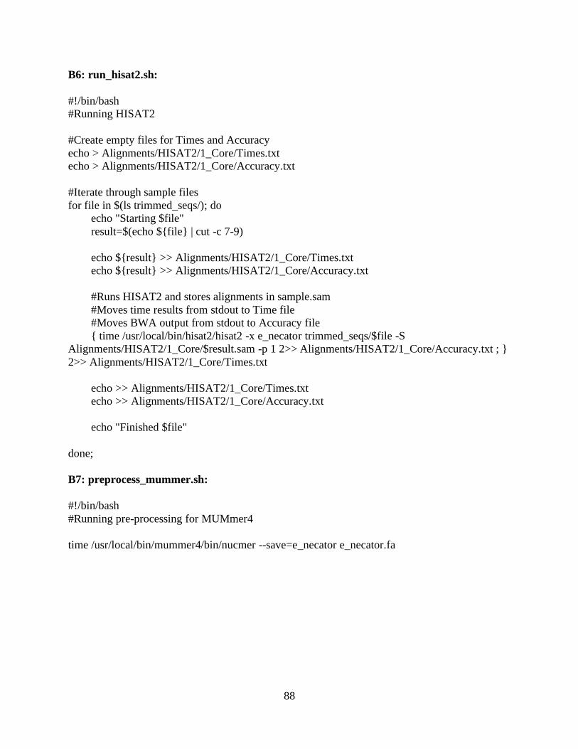
88

B6: run_hisat2.sh:

#!/bin/bash

#Running HISAT2

#Create empty files for Times and Accuracy

echo > Alignments/HISAT2/1_Core/Times.txt

echo > Alignments/HISAT2/1_Core/Accuracy.txt

#Iterate through sample files

for file in $(ls trimmed_seqs/); do

echo "Starting $file"

result=$(echo ${file} | cut -c 7-9)

echo ${result} >> Alignments/HISAT2/1_Core/Times.txt

echo ${result} >> Alignments/HISAT2/1_Core/Accuracy.txt

#Runs HISAT2 and stores alignments in sample.sam

#Moves time results from stdout to Time file

#Moves BWA output from stdout to Accuracy file

{ time /usr/local/bin/hisat2/hisat2 -x e_necator trimmed_seqs/$file -S

Alignments/HISAT2/1_Core/$result.sam -p 1 2>> Alignments/HISAT2/1_Core/Accuracy.txt ; }

2>> Alignments/HISAT2/1_Core/Times.txt

echo >> Alignments/HISAT2/1_Core/Times.txt

echo >> Alignments/HISAT2/1_Core/Accuracy.txt

echo "Finished $file"

done;

B7: preprocess_mummer.sh:

#!/bin/bash

#Running pre-processing for MUMmer4

time /usr/local/bin/mummer4/bin/nucmer --save=e_necator e_necator.fa

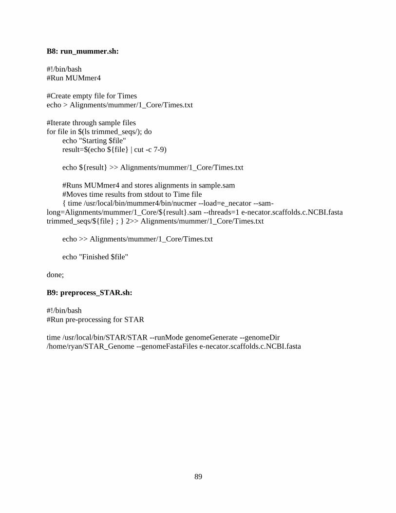
89

B8: run_mummer.sh:

#!/bin/bash

#Run MUMmer4

#Create empty file for Times

echo > Alignments/mummer/1_Core/Times.txt

#Iterate through sample files

for file in $(ls trimmed_seqs/); do

echo "Starting $file"

result=$(echo ${file} | cut -c 7-9)

echo ${result} >> Alignments/mummer/1_Core/Times.txt

#Runs MUMmer4 and stores alignments in sample.sam

#Moves time results from stdout to Time file

{ time /usr/local/bin/mummer4/bin/nucmer --load=e_necator --sam-

long=Alignments/mummer/1_Core/${result}.sam --threads=1 e-necator.scaffolds.c.NCBI.fasta

trimmed_seqs/${file} ; } 2>> Alignments/mummer/1_Core/Times.txt

echo >> Alignments/mummer/1_Core/Times.txt

echo "Finished $file"

done;

B9: preprocess_STAR.sh:

#!/bin/bash

#Run pre-processing for STAR

time /usr/local/bin/STAR/STAR --runMode genomeGenerate --genomeDir

/home/ryan/STAR_Genome --genomeFastaFiles e-necator.scaffolds.c.NCBI.fasta

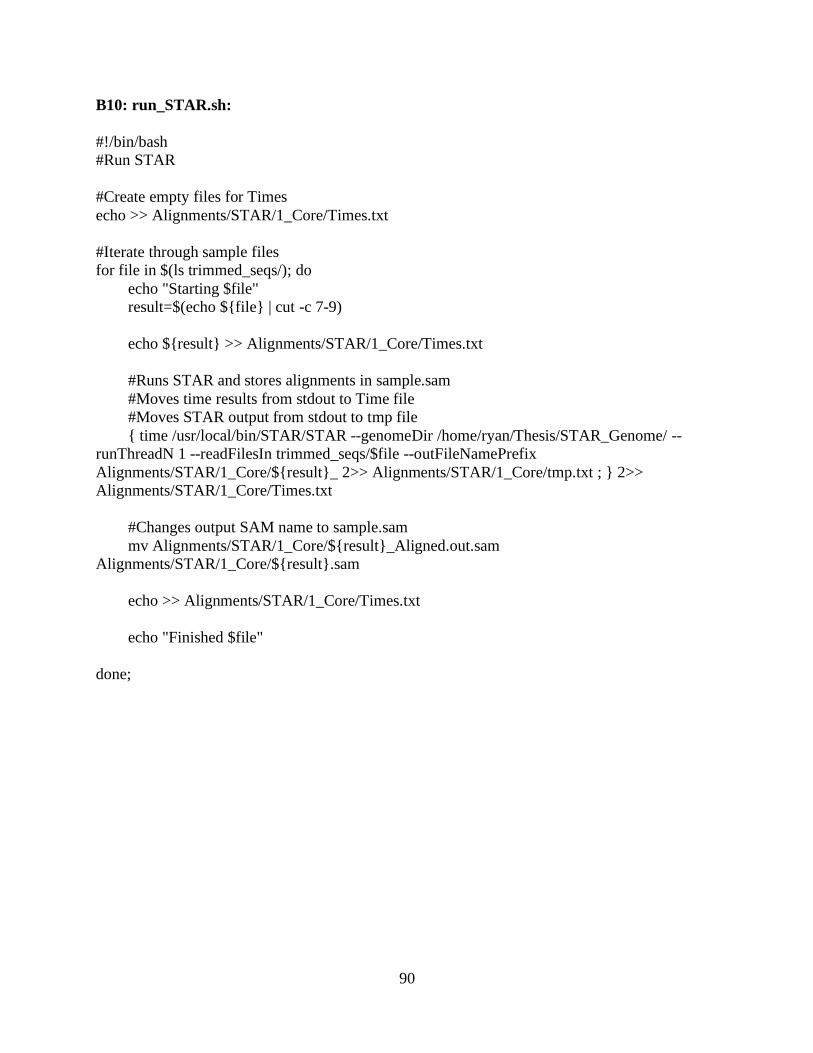
90

B10: run_STAR.sh:

#!/bin/bash

#Run STAR

#Create empty files for Times

echo >> Alignments/STAR/1_Core/Times.txt

#Iterate through sample files

for file in $(ls trimmed_seqs/); do

echo "Starting $file"

result=$(echo ${file} | cut -c 7-9)

echo ${result} >> Alignments/STAR/1_Core/Times.txt

#Runs STAR and stores alignments in sample.sam

#Moves time results from stdout to Time file

#Moves STAR output from stdout to tmp file

{ time /usr/local/bin/STAR/STAR --genomeDir /home/ryan/Thesis/STAR_Genome/ --

runThreadN 1 --readFilesIn trimmed_seqs/$file --outFileNamePrefix

Alignments/STAR/1_Core/${result}_ 2>> Alignments/STAR/1_Core/tmp.txt ; } 2>>

Alignments/STAR/1_Core/Times.txt

#Changes output SAM name to sample.sam

mv Alignments/STAR/1_Core/${result}_Aligned.out.sam

Alignments/STAR/1_Core/${result}.sam

echo >> Alignments/STAR/1_Core/Times.txt

echo "Finished $file"

done;

91

B11: run_tophat.sh:

#!/bin/bash

#Running TopHat2

export PATH=/usr/local/bin/bowtie2-2.3.5.1-linux-x86_64:$PATH

export BOWTIE_INDEXES=/home/ryan/Thesis

#Creates empty files for Times and Accuracy

echo > Alignments/Tophat/1_Core/Times.txt

echo > Alignments/Tophat/1_Core/Accuracy.txt

#Iterates through sample files

for file in $(ls tmp_seqs/); do

echo "Starting $file"

result=$(echo ${file} | cut -c 7-9)

echo ${result} >> Alignments/Tophat/1_Core/Times.txt

echo ${result} >> Alignments/Tophat/1_Core/Accuracy.txt

#Runs TopHat2 and stores alignments in sample.sam

#Moves time results from stdout to Time file

#Moves TopHat2 output from stdout to Accuracy file

{ time /usr/local/bin/tophat2/tophat -o Alignments/Tophat/1_Core/${result} -p 1 e_necator

tmp_seqs/$file 2>> Alignments/Tophat/1_Core/Accuracy.txt ; } 2>>

Alignments/Tophat/1_Core/Times.txt

echo >> Alignments/Tophat/1_Core_Anno/Times.txt

echo >> Alignments/Tophat/1_Core_Anno/Accuracy.txt

echo "Finished $file"

done;

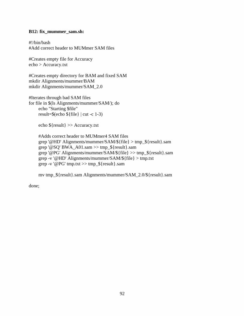
92

B12: fix_mummer_sam.sh:

#!/bin/bash

#Add correct header to MUMmer SAM files

#Creates empty file for Accuracy

echo > Accuracy.txt

#Creates empty directory for BAM and fixed SAM

mkdir Alignments/mummer/BAM

mkdir Alignments/mummer/SAM_2.0

#Iterates through bad SAM files

for file in $(ls Alignments/mummer/SAM/); do

echo "Starting $file"

result=$(echo ${file} | cut -c 1-3)

echo ${result} >> Accuracy.txt

#Adds correct header to MUMmer4 SAM files

grep '@HD' Alignments/mummer/SAM/${file} > tmp_${result}.sam

grep '@SQ' BWA_A01.sam >> tmp_${result}.sam

grep '@PG' Alignments/mummer/SAM/${file} >> tmp_${result}.sam

grep -v '@HD' Alignments/mummer/SAM/${file} > tmp.txt

grep -v '@PG' tmp.txt >> tmp_${result}.sam

mv tmp_${result}.sam Alignments/mummer/SAM_2.0/${result}.sam

done;

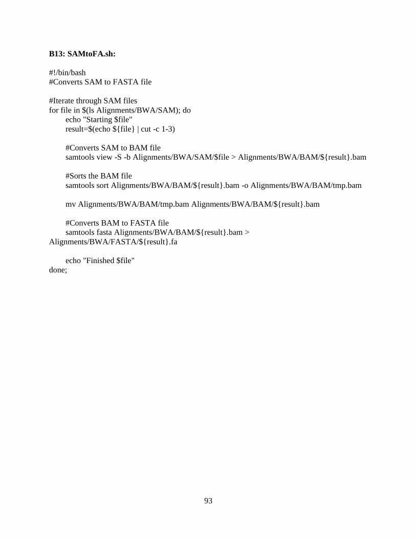
93

B13: SAMtoFA.sh:

#!/bin/bash

#Converts SAM to FASTA file

#Iterate through SAM files

for file in $(ls Alignments/BWA/SAM); do

echo "Starting $file"

result=$(echo ${file} | cut -c 1-3)

#Converts SAM to BAM file

samtools view -S -b Alignments/BWA/SAM/$file > Alignments/BWA/BAM/${result}.bam

#Sorts the BAM file

samtools sort Alignments/BWA/BAM/${result}.bam -o Alignments/BWA/BAM/tmp.bam

mv Alignments/BWA/BAM/tmp.bam Alignments/BWA/BAM/${result}.bam

#Converts BAM to FASTA file

samtools fasta Alignments/BWA/BAM/${result}.bam >

Alignments/BWA/FASTA/${result}.fa

echo "Finished $file"

done;