A Real-Time System for Color Sorting Edge-Glued Panel Parts

A Real-Time System for Color Sorting Edge-Glued Panel Parts

Qiang Lu

Thesis submitted to the Faculty of theVirginia Polytechnic Institute and State University

in partial fulfillment of the requirements for the degree of

Master of Sciencein

Electrical Engineering

Dr. Richard W. Conners, ChairDr. D. Earl Kline

Dr. A. Lynn AbbottDr. Ezra A. Brown

December 1, 1997Blacksburg, Virginia

Keywords: Color Sorting, Image Processing, Vision SystemCopyright 1997, Qiang Lu

A Real-Time System for Color Sorting Edge-Glued Panel Parts

Qiang Lu

(ABSTRACT)

This thesis describes the development of a software system for color sorting hardwoodedge-glued panel parts. Conceptually, this system can be broken down into three separateprocessing steps. The first step is to segment color images of each of the two part facesinto background and part. The second step involves extracting color information fromeach region labeled part and using this information to classify each part face as one ofa pre-selected number of color classes plus an out class. The third step involves usingthe two face labels and some distance information to determine which part face is thebetter to use in the face of an edge-glued panel. Since a part face is illuminated whilethe background is not, the segmentation into background and part can be done using verysimple computational methods. The color classification component of this system is basedon the Trichromatic Color Theory. It uses an estimate of a part’s 3-dimension (3-D) colorprobability function, P , to characterize the surface color of the part. Each color class isalso represented by an estimate of the 3-D color probability function that describes thepermissible distribution of colors within this color class. Let Pωi

denote the estimatedprobability function for color class ωi. Classification is accomplished by finding the colordifference between the estimated color probability function for the part and each of theestimated 3-D color probability functions that represent the color classes. The distancefunction used is the sum of the absolute values of the differences between the elements ofthe estimated probability function for a class and the estimated probability function of thepart. The sample is given the label of the color class to which it is closest if this distance isless than some class specific threshold for that class. If the distance to the class to whichthe part is closest is larger than the threshold for that class, the part is called an out.This supervised classification procedure first requires one to select training samples fromeach of the color classes to be considered. These training samples are used to generatePωi

for each color class ωi and to establish the value of the threshold Ti that is used todetermine when a part is an out. To aid in determining which part face is better to use inmaking a panel, the system allows one to prioritize the various color classes so that one ormore color classes can have the same priority. Using these priorities, labels for each of thepart faces, and the distance from each of the part faces’ estimated probability functionsto the estimated probability function of the class to which each face was assigned, thedecision logic selects which is the “better” face. If the two part faces are assigned to colorclasses that have different priorities, the part face assigned to the color class with higherpriority is chosen as the better face. If the two part faces have been assigned to the samecolor class or to two different classes having the same priority, the part face that is closest

to the estimated probability function of the color class to which it has been assigned ischosen to be the better face. Finally, if both faces are labeled out, the part becomes an outpart. This software system has been implemented on a prototype machine vision systemthat has undergone several months of in-plant testing. To date the system has only beentested on one type of material, southern red oak, with which it has proven itself capableof significantly out performing humans in creating high-quality edge-glued panels. Sincesouthern red oak has significantly more color variation than any other hardwood type orspecies, it is believed that this system will work very well on any hardwood material.

iii

Acknowledgments

I would like to thank my advisor, Dr. Richard W. Conners, for the immeasurable patienceand support throughout the course of my Master’s program. I would also like to thankDr. Earl Kline, Dr. Lynn Abbott, and Dr. Ezra A. Brown for their helpful advice andfor being on my committee. I am grateful to Philip A. Araman for his help and supportduring the initial period of this project.

I would like to thank Lichun Guo, Dr. Ray Bittner, and Dr. Xiangdong Liu for theirgreat help in my software design. I also wish to thank Dr. Thomas H. Drayer for hissupport in helping me understand the system hardware. I especially wish to thank SueEllen Cline and Bob Lineberry for their enormous technical support. I would like to thankKaren Ho, for her friendship and support during my entire Master’s program. Finally, Ithank Lori Hughes, Dr. Dave Kapp, and Mayukh Bhatta for their careful proof-reading ofthis thesis.

This thesis is in commemoration of my father, Prof. Zuyin Lu. I also dedicate thisthesis to my mother, Prof. Runsheng Zhu, for her love and encouragement. Finally, I wishto thank to my sister, Dr. Bin Lu, and my brother, Dr. Feng Lu, for their support andunderstanding.

iv

Contents

1 Introduction 1

1.1 Motivation . . . . . . . . . . . . . . . . . . . . . . . . . . . . . . . . . . . . 1

1.2 Objectives . . . . . . . . . . . . . . . . . . . . . . . . . . . . . . . . . . . . 6

1.3 Hypotheses and Limitations . . . . . . . . . . . . . . . . . . . . . . . . . . 7

1.4 Organization of Thesis . . . . . . . . . . . . . . . . . . . . . . . . . . . . . 9

2 Background 10

2.1 Human Perception of Color . . . . . . . . . . . . . . . . . . . . . . . . . . 10

2.2 Existing Color Sorting Methods . . . . . . . . . . . . . . . . . . . . . . . . 18

2.3 Conclusions . . . . . . . . . . . . . . . . . . . . . . . . . . . . . . . . . . . 20

3 Color Sorting and Better-Face Selection Algorithm 21

3.1 Choosing Color Representation . . . . . . . . . . . . . . . . . . . . . . . . 21

3.1.1 Introduction . . . . . . . . . . . . . . . . . . . . . . . . . . . . . . . 21

3.1.2 Estimated 3-D probability function method . . . . . . . . . . . . . 22

3.1.3 Estimated 1-D probability function method . . . . . . . . . . . . . 25

3.1.4 Average gray value method . . . . . . . . . . . . . . . . . . . . . . 26

v

3.1.5 Test Results and Conclusions . . . . . . . . . . . . . . . . . . . . . 28

3.2 Color Sorting Algorithms . . . . . . . . . . . . . . . . . . . . . . . . . . . . 39

3.2.1 Color sorting training algorithm . . . . . . . . . . . . . . . . . . . . 39

3.2.2 Real-time color sorting algorithm . . . . . . . . . . . . . . . . . . . 39

3.3 Better-Face Selection Algorithm . . . . . . . . . . . . . . . . . . . . . . . . 40

3.4 Reducing computational complexity for real-time sorting . . . . . . . . . . 41

4 System Hardware Overview 43

4.1 Introduction . . . . . . . . . . . . . . . . . . . . . . . . . . . . . . . . . . . 43

4.2 Image Processing System . . . . . . . . . . . . . . . . . . . . . . . . . . . . 45

4.2.1 Image processing computers . . . . . . . . . . . . . . . . . . . . . . 48

4.2.2 Parallel Port Communication . . . . . . . . . . . . . . . . . . . . . 50

4.2.3 Color line-scan camera . . . . . . . . . . . . . . . . . . . . . . . . . 54

4.2.4 Direct memory access image acquisition interface . . . . . . . . . . 58

4.2.5 Illumination sources . . . . . . . . . . . . . . . . . . . . . . . . . . 60

4.3 Sensing, Controlling, and Communicating . . . . . . . . . . . . . . . . . . 64

4.3.1 Overview . . . . . . . . . . . . . . . . . . . . . . . . . . . . . . . . 64

4.3.2 Control computer . . . . . . . . . . . . . . . . . . . . . . . . . . . . 65

4.3.3 Sensors . . . . . . . . . . . . . . . . . . . . . . . . . . . . . . . . . . 66

4.3.4 Lights and white targets . . . . . . . . . . . . . . . . . . . . . . . . 71

4.3.5 Serial communication . . . . . . . . . . . . . . . . . . . . . . . . . . 74

4.4 Remote Debugging Auxiliary Facilities . . . . . . . . . . . . . . . . . . . . 74

vi

5 The System Software 77

5.1 System Software Overview . . . . . . . . . . . . . . . . . . . . . . . . . . . 77

5.2 User Interface . . . . . . . . . . . . . . . . . . . . . . . . . . . . . . . . . . 77

5.3 System Setup and Light Control . . . . . . . . . . . . . . . . . . . . . . . . 79

5.3.1 System setup functions . . . . . . . . . . . . . . . . . . . . . . . . . 81

5.3.2 Shading correction data collection . . . . . . . . . . . . . . . . . . . 86

5.3.3 Light intensity checking . . . . . . . . . . . . . . . . . . . . . . . . 88

5.4 Color Sorting . . . . . . . . . . . . . . . . . . . . . . . . . . . . . . . . . . 91

5.4.1 System training . . . . . . . . . . . . . . . . . . . . . . . . . . . . . 92

5.4.2 Real-time color sorting . . . . . . . . . . . . . . . . . . . . . . . . . 95

6 System Performance Testing 97

6.1 Introduction . . . . . . . . . . . . . . . . . . . . . . . . . . . . . . . . . . . 97

6.2 Preliminary Testing . . . . . . . . . . . . . . . . . . . . . . . . . . . . . . . 98

6.3 In-plant Testing . . . . . . . . . . . . . . . . . . . . . . . . . . . . . . . . . 98

6.3.1 Problems encountered . . . . . . . . . . . . . . . . . . . . . . . . . 98

6.3.2 Making the prototype machine industrially robust . . . . . . . . . . 100

6.3.3 Further system improvement . . . . . . . . . . . . . . . . . . . . . . 101

6.3.4 In-plant color-sorting result . . . . . . . . . . . . . . . . . . . . . . 102

6.4 Conclusions . . . . . . . . . . . . . . . . . . . . . . . . . . . . . . . . . . . 105

7 Future Research 106

vii

List of Figures

1.1 A typical wood part . . . . . . . . . . . . . . . . . . . . . . . . . . . . . . 2

1.2 More detail on a typical wood part . . . . . . . . . . . . . . . . . . . . . . 3

1.3 A suggested prototype real-time color sorting system . . . . . . . . . . . . 5

1.4 Typical grain patterns. . . . . . . . . . . . . . . . . . . . . . . . . . . . . 8

2.1 A typical set of color sensitivity curves . . . . . . . . . . . . . . . . . . . . 11

2.2 A color in a unnormalized 3-D color space . . . . . . . . . . . . . . . . . . 13

2.3 A color in a normalized 3-D color space . . . . . . . . . . . . . . . . . . . . 13

2.4 A color in a normalized 2-D color space . . . . . . . . . . . . . . . . . . . . 14

2.5 The C.I.E. spectrum locus . . . . . . . . . . . . . . . . . . . . . . . . . . . 14

2.6 The diagram of CIE chromaticities . . . . . . . . . . . . . . . . . . . . . . 15

2.7 The concepts of hue, saturation and lightness. . . . . . . . . . . . . . . . . 17

3.1 The nonzero elements of an estimated 3-D probability function P shown inr-g-b color space. . . . . . . . . . . . . . . . . . . . . . . . . . . . . . . . . 23

3.2 Estimated 1-D probability functions . . . . . . . . . . . . . . . . . . . . . . 27

3.3 Training samples of color class A . . . . . . . . . . . . . . . . . . . . . . . 29

3.4 Training samples of color class B . . . . . . . . . . . . . . . . . . . . . . . 30

viii

3.5 Training samples of color class CL . . . . . . . . . . . . . . . . . . . . . . . 30

3.6 Training samples of color class CM . . . . . . . . . . . . . . . . . . . . . . 31

3.7 Training samples of color class CD . . . . . . . . . . . . . . . . . . . . . . 31

3.8 Training samples of color class D . . . . . . . . . . . . . . . . . . . . . . . 34

3.9 A panel composed by parts from color class A. . . . . . . . . . . . . . . . . 35

3.10 A panel composed by parts from color class B. . . . . . . . . . . . . . . . . 35

3.11 A panel composed by parts from color class CL. . . . . . . . . . . . . . . . 36

3.12 A panel composed by parts from color class CM. . . . . . . . . . . . . . . . 36

3.13 A panel composed by parts from color class CD. . . . . . . . . . . . . . . . 37

3.14 A panel composed by parts from color class D. . . . . . . . . . . . . . . . . 37

3.15 Parts classified as out. . . . . . . . . . . . . . . . . . . . . . . . . . . . . . 38

3.16 The side selected by Better-face selection algorithm. . . . . . . . . . . . . . 41

3.17 The side not selected by Better-face selection algorithm. . . . . . . . . . . . 41

4.1 System diagram . . . . . . . . . . . . . . . . . . . . . . . . . . . . . . . . . 44

4.2 The outward appearance of the color sorting system . . . . . . . . . . . . . 46

4.3 The outward appearance of the color sorting system from another view angle 47

4.4 Parallel port communication pin specifications . . . . . . . . . . . . . . . . 52

4.5 A closer view of the camera and lights. . . . . . . . . . . . . . . . . . . . . 55

4.6 The linescan camera controller. . . . . . . . . . . . . . . . . . . . . . . . . 56

4.7 The high speed data transfer interface board. . . . . . . . . . . . . . . . . 59

4.8 A light source. . . . . . . . . . . . . . . . . . . . . . . . . . . . . . . . . . . 61

4.9 Inside view of the cabinet. . . . . . . . . . . . . . . . . . . . . . . . . . . . 62

ix

4.10 Infrared object detect sensor . . . . . . . . . . . . . . . . . . . . . . . . . . 67

4.11 Infrared and ultrasonic sensors. . . . . . . . . . . . . . . . . . . . . . . . . 68

4.12 The ultrasonic sensor. . . . . . . . . . . . . . . . . . . . . . . . . . . . . . 70

4.13 The informational lights used to display color sorting results. . . . . . . . . 73

4.14 The illustration of Point-to-Point Protocol . . . . . . . . . . . . . . . . . . 75

5.1 Graphic user interface menu tree . . . . . . . . . . . . . . . . . . . . . . . 78

5.2 Hardware used for scanning one part face . . . . . . . . . . . . . . . . . . . 80

5.3 A GUI page used for camera and lighting controls. . . . . . . . . . . . . . . 83

5.4 A GUI page used for training sample scanning. . . . . . . . . . . . . . . . . 93

6.1 The variations of light . . . . . . . . . . . . . . . . . . . . . . . . . . . . . 103

x

List of Tables

1.1 Possible Definition for Color Groups of Southern Red Oak . . . . . . . . . 3

3.1 Color Class Definitions . . . . . . . . . . . . . . . . . . . . . . . . . . . . . 29

3.2 Estimated 3-D Probability Function Method Partial Test Result . . . . . . 32

3.3 Estimated 1-D Probability Function Method Partial Test Result . . . . . . 33

4.1 Parallel Port Pin Specifications . . . . . . . . . . . . . . . . . . . . . . . . 53

6.1 In-Plant Color Sorting Result . . . . . . . . . . . . . . . . . . . . . . . . . 104

xi

Chapter 1

Introduction

1.1 Motivation

The hardwood forest products industry is facing a number of major problems. Chief amongthese is the ever increasing cost of raw materials and the difficulty in hiring and retaininghighly skilled and motivated employees. These difficulties are forcing the industry to lookfor better processing methods, which reduce labor costs, improve the recovery of usefulparts from raw materials, and/or improve product quality.

A labor-intensive and difficult task required in manufacturing a number of hardwoodproducts is the color sorting of parts used to create edge-glued panels. Edge-glued panelsare used to make such items as door fronts, table tops, and desk tops. Edge-glued panelsare used whenever it is impossible to get a single piece of wood of the right dimensionsand/or whenever dimensional stability is important. Edge-glued panels are much more di-mensionally stable than a single piece of wood with the same overall dimensions. The smallpieces composing each panel are called parts (Figure 1.1). Each part has two faces, the topface and the bottom face. Panel parts vary in length depending on the dimensions of thepanel they will form. They typically have random widths ranging from one to six inches,again depending on the dimensions of the panel they will be used to create. Obviouslythey can also vary in thickness, again depending on the desired thickness of the panel theywill be used to create. A part’s sides are called edges. If this part is fed on a conveyor, thefront edge, which is perpendicular to the moving direction, is called the leading edge, andthe back edge, which is perpendicular to the moving direction, is the trailing edge. Figure1.2 illustrates a typical edge-glued panel.

1

Qiang Lu Chapter 1. Introduction 2

top surface

bottom surface

side edges

leading (trailing) edge

trailing (leading) edge

moving direction

Figure 1.1: A typical wood part.

The color sorting or matching of panel parts is done in an attempt to assure that thefront side of edge-glued panels will have a relatively uniform color. The ability to createsuch uniformly colored panels is very important because buyers of hardwood products de-mand that these products have consistent color characteristics.

There are two ways manufacturers can generate such uniformly colored panels. The firstinvolves establishing several different color classes, which tend to span the color character-istics of the material to be processed. For example, when using southern red oak, parts canbe shades of red, green, brown, or white. Thus, for southern red oak four color groupingsare possible. Call these color classes A, B, C and D, where these classes correspond to thered, green, brown, and white color characteristics respectively (see Table 1.1). Operatorsattempt to sort a part into one of these color classes. They do so by placing the part intoa bin holding parts for that color class. To create color-matched panels, operators at theglue reels use parts from one bin at a time to form panels. This method is called colorsorting.

The second way to generate uniformly colored panels is to have an operator pick up aload of parts. The number of parts that comprise a load may range from 700 to 900. Tocreate a panel, the operator first selects a seed part and then attempts to grow a panelaround the seed by selecting parts that closely match the seed’s color. Part by part, thepanel is built until it has the appropriate width. Typically, several panels are being grown


glued-edges

panel surface

Figure 1.2: A typical panel composed of four parts which are glued on the edges.

Table 1.1: Possible Definition for Color Groups of Southern Red Oak

Color Group A B C DCharacteristic red green brown white


at the same time. If a part from the load is selected which does not go with any of thepanels being created, a new panel is started using this part as the seed. With this method,color matching, parts are matched by color.

These two methods, color sorting and color matching, are the most commonly usedprocedures for creating uniformly colored panels. Color sorting is relatively easy and quickto perform, but the quality of each panel created is low, since panels in the same bin canhave significant variations in color. Humans can reliably sort parts into only a limitednumber of classes. Color matching typically creates much higher quality panels, althoughit is much more labor intensive. It also requires much more plant floor area since space isneeded for the processing of several panels simultaneously. Since most plants must operatequickly and lack free floor space, most high volume manufacturers use the color sortingmethod.

Consistent color sorting of edge-glued panel parts is known to be a difficult task forhumans to perform. This is especially true as more and more buyers are choosing hard-wood products that have clear or very lightly stained finishes. Such finishes do not hidevariations in color of the panel parts as dark stains do. Hence the color sorting must bevery precise to obtain the desired consistency in panel color, parts must be sorted into alarge number of color classes with adjacent color classes having very similar color char-acteristics. The number of color classes used depends on the type of hardwood lumber.The slight differences that separate the color classes and the demands of management forhigh throughput makes the color sorting job one of the least favorite among plant personnel.

To understand the importance of color sorting to hardwood plant management, mostoperations grade edge-glued panels into at least three output categories: clear, acceptable,and unacceptable. Clear panels have approximately the same color across their better faceand are the most valuable panels. Acceptable panels have color characteristics that arewithin acceptable bounds but are not uniform. Unacceptable panels have color characteris-tics which vary widely across their best face and do not produce an acceptable panels evenunder a dark stain.

The success of the panel making operation depends on the percentages of clear, accept-able, and unacceptable panels produced. Since increasing the percentage of clear panelsimproves profit margins, the goal of management must be to create as many clear panelsas possible. One possible way of increasing the number of clear parts is to automate thecolor sorting operation using a machine vision system to make the sorting decisions. This


automated process would remove the affects of fatigue, boredom, and stress known to affectthe decision-making performance of plant personnel.

object moving direction

line scan camera

object

IBM PC

camera cable

Figure 1.3: A suggested prototype for a real-time color sorting system.

A possible machine vision system for performing the color sorting operation is shownin Figure 1.3. This system has four basic components: a color line-scan camera, an analog-to-digital (A/D) converter, a computer, and a materials handling system for moving partsthrough the color camera’s field of view. When a part passes through the line-scan camera’sfield of view, the camera scans one image line at a time and collects analog color imagedata. The A/D converter converts the analog color image signals into digital signals that a


computer can understand. The computer receives and stores the digital color image data.After an image of the entire part has been created, the computer applies algorithms thatcolor-sort this object in real time. The computer must be able to execute these algorithmsin less than 3 seconds to meet a typical plants throughput requirements.

The goal of this thesis is to create a software system that can perform this difficultcolor-sorting task and that can control the hardware components of the machine visionsystem. The software color-sorting system must sort parts into a pre-selected number ofcolor classes, which must be defined so that any part in a class can be combined with anyother part in the class to create a clear panel. The color sorting algorithms must run inunder 3 seconds to meet throughput requirements. The software must control all hardwarefunctions and detect hardware malfunctions so that corrective action can be taken.

1.2 Objectives

Given the above, the primary objective is to create a real-time software color-sorting sys-tem for edge-glued panel parts including the control software for managing the hardwarecomponents of the complete machine vision system. More specifically, the objectives arestated as follows:

1. To create a software system for color sorting hardwood edge-glued panel parts. Thisgoal includes developing the computer algorithms required to make sorting decisionsand software for controlling hardware components needed to acquire and process colorimage data;

2. To implement this software system on a prototype sorting system that can be oper-ated in a manufacturing plant at reasonable processing speeds. The purpose of theprototype is to verify that the software methodologies developed will perform satis-factorily in an industrial environment where dust, temperature variations, and powerfluctuations can affect the imaging, lighting, and computer components. Integratingthis software into the prototype includes creating a user-friendly interface so the sys-tem can be operated by plant personnel. This goal also involves modifying the basicalgorithms so that they will run as fast as possible and includes developing softwarefor monitoring the system so that potential problems, e.g., a burnt out light bulb,can be detected as quickly as possible;


3. To conduct in-plant tests to verify system performance, including training plant per-sonnel to help locate system problems, and creating a dial-up facility for the plantso that on-line consultations about system performance and/or problems can be pro-vided.

To achieve the above performance requirements, a number of vision methodologies hadto be incorporated into this real-time system. These methodologies will be discussed inChapter 2 through Chapter 6.

1.3 Hypotheses and Limitations

Little is known about the human perception of color [99]. Studies suggest that it is highlynonlinear, and it has proved difficult to model [99]. It is true that a number of successfulcommercial color matching systems have been developed [57, 97, 47, 96, 88, 79, 6, 22, 82,35, 90, 99, 85, 78], e.g., systems for matching paint. However, these systems have all beendeveloped to match items that have a uniform color. Wood is not uniform in color; ithas grain patterns (Figure 1.4) as well as low frequency color variations across its surface.Hence, given what is known about human color perception, it seems difficult to createsimple methods for modeling human color perception involved in sorting hardwood parts.The underlying hypothesis of this work is that computationally simple methods for colormatching hardwood parts can be created.

There are a number of limitations to this study. The first limitation is that only onetype of hardwood material, southern red oak, will be considered. Fortunately, southernred oak has as much or more color variation than any other type of hardwood material.Therefore, it can be argued that if the methods developed work well on southern red oak,they should also work well on other types of hardwood material.

Other possible limitations result from the assumption that all the parts will be of onethickness, skipped-planed, and free of mineral streak. The single thickness assumption usedin creating the hardware components of the system means that a fixed imaging geometrycan be used. It does not affect the generality of the results produced by the software sys-tem described here, however, since typically only one thickness of material is processed ata time. It would therefore be possible to adjust camera and light source height betweenruns to accommodate parts of a different thickness if an adjustable imaging geometry was


Figure 1.4: Typical grain patterns.


provided by the hardware components. The restriction to parts that have been skippedplaned is also justifiable; most hardwood plants already skip-plane their parts prior to colorsorting to aid their employees in performing this difficult task.

The limitation of the system to parts that do not contain mineral streak is, however,a problem. Most manufacturers will allow some mineral streak in their edge-glued panelparts. Doing so allows them to get an improved yield of these parts from a given volumeof lumber. Modifying the system to handle mineral streak is a topic for future research.

1.4 Organization of Thesis

Chapter 2 presents the background for this work, which includes a discussion of what isknown about human color perception and of the efforts that have been made to color matchvarious types of materials. Based on the information presented in Chapter 2, Chapter 3presents a number of possible ways to do the color matching. The relative merits anddemerits of the various approaches presented are given and the details of the 3-dimensionalprobability function-based algorithm are described. Chapter 4 is a description of the pro-totype hardware system. Chapter 5 discusses the implementation of the software systemon this prototype, including the tree structure of the menu-driven human interface and thesystem utilities. Chapter 6 outlines the results of the in-plant testing. Chapter 7 presentssome direction for future research.

Chapter 2

Background

2.1 Human Perception of Color

Studies of the human vision system indicate that the human perception of color is a verycomplicated process [99]. Psychologists who have studied human color perception agreethat the incoming light causes chemical and electrical reactions in the human eye, allowingthe signals produced to be transferred to the brain by the optic nerve [99]. These signalsare then reconstructed in the human brain, perhaps at the level of the visual cortex, sopeople can sense the outside world [99]. Emulation of the processes of human perceptionhas proven to be very difficult to create. However, some mathematical models that seem-ingly describe some aspects of human color perception have been created. These modelsattempt to describe aspects of human judgements of the similarity of colors.

Three coordinate systems are commonly used to model human color similarity judge-ments: r-g-b index representation; [XYZ] coordinate system; and hue, saturation and light-ness color description space. All these models have proven useful in modeling humanjudgements of color similarity and have a common basis in the Trichromatic Color Theory.By using these systems, the highly non-linear nature of human color perception is easilydisplayed.

Trichromatic Color Theory is the fundamental theory for color perception and was for-mulated by the Commission Internationale de l’Eclairage(C.I.E.) in 1931. Its formulationis based on a extensive series of experimental measurements by the C.I.E. [14]. This the-

10

Qiang Lu Chapter 2. Background 11

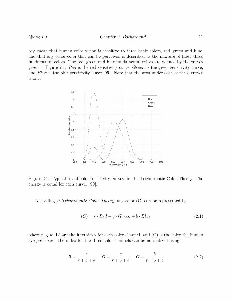
ory states that human color vision is sensitive to three basic colors, red, green and blue,and that any other color that can be perceived is described as the mixture of these threefundamental colors. The red, green and blue fundamental colors are defined by the curvesgiven in Figure 2.1. Red is the red sensitivity curve, Green is the green sensitivity curve,and Blue is the blue sensitivity curve [99]. Note that the area under each of these curvesis one.

350 400 450 500 550 600 650 700 750 8000

0.2

0.4

0.6

0.8

1

1.2

1.4

1.6

1.8

Wavelength (nm)

Rel

ativ

e se

nsiti

vity

Red

Green

Blue

Figure 2.1: Typical set of color sensitivity curves for the Trichromatic Color Theory. Theenergy is equal for each curve. [99].

According to Trichromatic Color Theory, any color (C) can be represented by

(C) = r · Red+ g ·Green+ b · Blue (2.1)

where r, g and b are the intensities for each color channel, and (C) is the color the humaneye perceives. The index for the three color channels can be normalized using

R =r

r + g + b, G =

g

r + g + b, G =

b

r + g + b(2.2)


where R, G and B are the normalized relative intensities for each color channel. Note thatthe R-G-B system does not contain all the information that the r-g-b system does, sincebrightness or intensity information implicit in the definition of r-g-b (Equation 2.1) is lostin the transformation defined by Equation 2.2. The C.I.E. tests were done using Equation2.2 since, in these experiments, constant brightness illuminants were used. Hence, therewas no need to put brightness information into the color equation; doing so would onlyincrease the computation burden. A straightforward consequence of Equation 2.2 is that

R +G+B = 1 (2.3)

Therefore, according to Trichromatic Color Theory, a color (C) can be expressed ineither a r-g-b three-dimensional (Figure 2.2) or a R-G-B three dimensional space (Figure2.3). Figure 2.3 depicts the normalized 3-D color space. Figure 2.4 is a compressed 2-Dversion of Figure 2.3. In the compressed space shown in Figure 2.4, the horizontal axisis the red component index, R, and the vertical axis is the green component index, G.Note that the third component, the blue component B, does not appear. To get the Bcomponent value from this compressed representation one must use

B = 1−R−G (2.4)

a relationship that follows directly from Equation 2.3.

Furthermore, a spectrum locus is drawn on the compressed 2-D color space (Figure 2.5).Inside the spectrum locus are the colors visible to human vision. The triangle along the linesof the spectrum locus composes a new coordinate system, the [XYZ] system. The originsof this triangle are marked as [X], [Y ] and [Z] on Figure 2.5. There is a transformationmatrix between R-G-B coordinates and the [XYZ] coordinates. Figure 2.6 shows the new[XYZ] system transformed from the R-G-B system inside the triangle of Figure 2.5.

Using the [XYZ] system, the C.I.E. measured the relative sensitivity of the human per-ceptual system to different colors. All the colors within the range of each ellipse in Figure2.6 are perceived as the same color by the human perceptual system. As can easily beobserved, the size and shape of these ellipses varies with position within the [XYZ] space.This suggests that the human perception of color is nonlinear and varies across the range


050

100150

200250

0

50

100

150

200

2500

50

100

150

200

250

redgreen

blue

(C)

Figure 2.2: A color (C) in r-g-b index color system expressed in a 3-D color space withunnormalized values.

00.2

0.40.6

0.81

0

0.2

0.4

0.6

0.8

10

0.2

0.4

0.6

0.8

1

redgreen

blue

(C)

Figure 2.3: A color (C) in R-G-B color index system expressed in a 3-D color space withnormalized values.


0 0.1 0.2 0.3 0.4 0.5 0.6 0.7 0.8 0.9 10

0.1

0.2

0.3

0.4

0.5

0.6

0.7

0.8

0.9

1

(C)

red

gree

n

Figure 2.4: The color (C) in R-G-B color index system expressed in a 2-D color space.

[G]

[X]

0.50

[Z]

[B] 1.0

[R}

-1.0-2.0

1.0

2.0

0.60um

0.58

0.56

0.53

0.520.51

0.49

Spectrumlocus

[Y]

0.48

0.47

Figure 2.5: The spectrum locus on the compressed 2-D color space.[99].


[Y]

axis

red

pink

cool white

deep blue

blue

gold

green

780

620

600

560

540

520

510

500

490

480

470

380

.0 .8

.9

[X] axis

Equal EnergyPoint of

(wavelength in nm)Spectral energy locus

daylight

warm white

Figure 2.6: The diagram of CIE chromaticities. The colors in the same ellipse are perceivedas the same color by a standard observer [44].


of perceivable colors.

Theoretically, it is possible to incorporate this obvious nonlinearity into a color match-ing algorithm. Consider, for example, the inspection of plastic parts used in automobileinteriors. Each of these components has a uniform color, and there is a small set of targetcolors. Each component must be matched to one of the set of target colors, i.e., the targetinterior colors for a model year. To incorporate the nonuniformity, experiments on humansubjects could be performed to establish the ellipse size and orientation for each of thetarget colors. A spectrometer reading of each plastic part could then be taken. A trans-formation from the spectrometer’s R-G-B space readout to [XYZ] space could be appliedto a reading. The resulting point in [XYZ] space could be checked to see in which ellipsethe part’s color lies.

Unfortunately, creating this algorithm involves a lot of work. Therefore, color matchingdone in the textile and plastics industry ignores this obvious nonlinearity in human visionand merely compares how closely the R-G-B space color of a part is to the R-G-B spaceprototypical colors of the various color classes [97]. If two points in R-G-B space are closertogether than a predetermined threshold, the colors are said to match. Such algorithmshave been used for years, and all are based on the Trichromatic Color Theory.

The last way of measuring color described here is illustrated in Figure 2.7. This 3-dimensional color space is also based on the Trichromatic Color Theory, and the conceptsof hue, saturation and lightness are introduced. The central vertical axis represents thelocus of grays, with black at the lower and white at the upper extremity. The distancefrom black to white fixes the scale of the solid. A color of any one hue can be locatedin a horizontal plane with the vertical axis as center. The height of a sample above theblack level indicates by its lightness, while the horizontal distance from the black and whitevertical axis indicates its saturation. If the plane is assumed to rotate around this axis,it will pass through successive hues of red, orange, yellow, etc. A mapping will transformthis geometrical color space into the [XYZ] system; hue, saturation, and lightness canbe converted into the [XYZ] indices and, hence, into R-G-B space coordinates as well.The geometrical color space can also be converted into r-g-b space coordinates. From aninformation content point of view, both the r-g-b and the hue, saturation, and lightnesscoordinate systems contain intensity information while the R-G-B and [XYZ] spaces donot.

The hue, saturation, and lightness space representation is popular with the electronic


Black

Red

Hue

White

Green

Blue

Lig

htne

ss

Saturation

Figure 2.7: The concepts of hue, saturation and lightness in a three-dimensional figure [99].


display industry, e.g., color of television sets is adjusted by hue, saturation, and lightness,which is the dimension of color experience related to the amount of light emitted by anobject. The hue is the dimension of color experience that distinguishes among red, orange,yellow, green, blue, and so on; it is the dimension of color most strongly determined bylight’s wavelength. The saturation is the dimension of color experience that distinguishespale colors from vivid colors [87].

This representation has been used in several scene analysis systems [23] that have beendesigned to analyze outdoor scenes. These systems attempt to segment such scenes byfinding the regions that have differences in their hue and saturation. This color coordinatesystem is a very natural one to use for this application since shadows are important inoutdoor scenes. Theoretically, the hue and saturation of an object will not change as onemoves from its fully illuminated areas to areas that are in shadow.

Each coordinate system has its own advantages and disadvantages. In this work ther-g-b color space was selected over the other three systems for use on the color matchingproblem because lightness and darkness information, i.e., intensity information, is impor-tant in the human color matching of edge-glued panel parts. The [XYZ] and R-G-B spacesdo not contain any intensity information. Therefore, it was judged that neither of thesetwo systems should be employed. While the hue, saturation, and brightness system doescontain intensity information, typical color imaging sensors do not output pixels in thiscoordinate system. Hence, each color pixel in an image would have to be transformed bythe sensor from the r-g-b system output into hue, saturation, and brightness. Given thevolume of image data that must be analyzed and the short time available to do the anal-ysis, the only compelling reason for using the hue, saturation, and lightness system stemsfrom the invariance of a color’s hue and saturation in shadows, which is the reason thiscolor coordinate system is used in outdoor scene analysis systems. However, in this colormatching work, this invariance is unimportant. Therefore, the r-g-b coordinate system isused.

2.2 Existing Color Sorting Methods

A number of papers have been published on color matching of fabric for the textile industry.The most commonly used algorithm in these papers is similar to the one described above inwhich a spectrometer is used to obtain a r-g-b color coordinate for the fabric being inspected.


This color coordinate is then compared to the r-g-b color coordinates of the prototypes foreach of the color classes. A difference measure is used to determine how far the fabric’s coloris from each of the prototypical colors, and the color is given the label of the prototypicalcolor class to which it is closest [64, 60, 40, 57, 97, 47, 96, 88, 79, 6, 22, 82, 35, 90, 99, 85, 78].

Measuring the quantity of color difference is a further application of color. A number ofresearchers have applied the hue-saturation diagram comparison method [11, 7, 42, 30, 31,2, 3, 74, 34, 45, 1, 98, 41]. Unfortunately most of these articles only considered the colorcharacteristics of uniformly colored surfaces.

Color matching of wood parts is more complicated than color matching uniformly col-ored parts because the color of a wood part varies across its surface. This color variation iscaused by not only grain pattern but also low frequency variations across a part’s surface.Fortunately, these variations in color are typically not very pronounced, which might sim-plify the color matching task. A number of possible algorithms for color matching woodparts have been proposed in the literature [103, 57, 16, 19, 21, 26, 27, 10, 50, 51, 52, 53,54, 55, 56, 68, 93, 8, 91, 92, 95]. Of the methods that have been suggested, two approachesstand out. One of the most attractive methods is the mean value method [103]. It suggeststhat a wood part’s surface color characteristics can be represented by the mean value ofeach color channel in the r-g-b color space. The difference between the mean values fortwo different wood parts indicates possible difference in the parts’ color characteristics. Tosort parts into several color classes requires only that the part’s mean values for r-g-b becomputed and compared to the r-g-b values that characterize the color of each color class.The underlying assumption with this algorithm is that the smaller the computed differencevalue is, the better the part fits into the color class. Hence, the part is given the label of thecolor class to which it is closest in r-g-b color space. This method is attractive because it isconceptually straightforward and computationally simple. Unfortunately, the test resultsreported by the author suggest that this methodology is incapable of performing the typesof sorts required in sorting edge-glued panel parts.

Another promising algorithm is the 1-D histogram method [4]. Instead of using the meanvalue to represent the color characteristic of each color channel, three 1-D histograms, onehistogram for each color channel are used. The rest of the algorithm is similar to the meanvalue method and is described in [4], which does not give any test results. While beingmore computationally complex than the mean value method, the 1-D histogram method isstill a conceptually simple method.


2.3 Conclusions

A number of color representation methods were described and all of these methods arebased on Trichromatic Color Theory. Of the methods described, the one that seems themost appropriate for the color matching of edge-glued panel parts is the r-g-b representationbecause lightness and darkness are believed to be important in the human perception ofcolor difference of wood parts. Therefore, the R-G-B and [XYZ] are immediately eliminatedfrom consideration since those two representations do not capture differences in lightnessand darkness. Though the hue, saturation, and brightness representation does contain allthe needed information just as the r-g-b representation does, it requires that every colorpixel be transformed from r-g-b space to the hue, saturation, and brightness space. Thistransformation imposes a computational burden that can be justified only if there is somegain involved by considering this space, e.g., the gain obtained when this coordinate systemis used in the analysis of outdoor scenes. In the color matching problem considered here, itdoes not appear advantageous to transform r-g-b space to hue, saturation, and brightnessspace.

Finally, two potential algorithms for color matching edge-glued panel parts were foundin the literature. Both are conceptually and computationally simple. Prudence demandsthat these algorithms be explored.

Chapter 3

Color Sorting and Better-FaceSelection Algorithm

In this chapter, the color sorting algorithm and better-face selection algorithm are describedin detail. Section 3.1 discusses the selection of a color representation for a part face. Section3.2 discusses the color sorting training algorithm and real-time color sorting algorithm. Todetermine which of the two part faces is the better one to appear on the outer surface, abetter face selection algorithm is required. Section 3.3 describes such an algorithm. Sec-tion 3.4 discusses ways of reducing computation complexity to increase the throughput ofreal-time sorting.

3.1 Choosing Color Representation

3.1.1 Introduction

The key to successfully color sorting panel parts is define a color representation that canaccurately gauge all the natural color variations that occurs in wood. The algorithm em-ploying this representation must also be computationally simple to make real-time operationpossible.

Earlier three possible color representations for color sorting panel parts were identified.

21

Qiang Lu Chapter 3. Color Sorting and Better-Face Selection Algorithm 22

These include the estimated 3-D probability function method, the estimated 1-D probabilityfunction method, and the average gray value method. The following three sections will de-scribe these three methods in detail and discuss the relative merits and demerits of eachmethod. Then test results will be given that compares the relative capabilities of each ofthese representations. Based on these test results, the color representation used in the colorsorting system is selected.

3.1.2 Estimated 3-D probability function method

The major problem in color sorting wood parts is the fact that a face of a part is not oneuniform color but rather is comprised of many colors. There are color differences betweenearly wood and late wood that produce the annular ring structure in wood. There arelow frequency variations in color across a part’s width and down its length. Any colorrepresentation used to sort wooden parts must capture these variations since the variationsare known to affect the perceived color of the part.

Perhaps the most straightforward way of capturing the “distribution” of colors thatoccur in a part face is to use a 3-D color histogram, H , i.e.,

H = [h(r, g, b)] (3.1)

where h(r, g, b) is the number of pixels of the part face that has color (r, g, b). Unfortunately,while H does capture the distribution of colors comprising a face, two 3-D histogramscomputed from different sized parts but parts which have similar distributions of colorwill be markedly different. The difference results from the fact that the total number ofpixels appearing on each part could be very different. To remove this size dependence,the preferred way to represent the distribution of color on a part face is to use the 3-Destimated probability function, P = [p(r, g, b)], where

p(r, g, b) = h(r, g, b)/N (3.2)

and where


N =∑r

∑g

∑b

h(r, g, b). (3.3)

Figure 3.1 shows the nonzero estimated probability function P computed from a faceof a red oak part. This face is part of what will be called later in this chapter the red colorclass. In this figure, ◦ denotes elements of P with values greater than 0, and less than0.01, × denotes elements with values greater than or equal to 0.01 and less than 0.02, andb denotes elements with values greater than or equal to 0.02 but less than 0.03.

0

10

20

30

40

50

600

1020

3040

5060

0

10

20

30

40

50

60

red green

blue

b − more than 2% but less than 3%x − more than 1% but less than 2%o − less than 1%

Figure 3.1: The nonzero elements of an estimated 3-D probability function P shown inr-g-b color space. This P was computed from an image of a part from the red color class.

Let P1 = [p1(r, g, b)] be the 3-D estimated probability function computed from onepart face, and P2 = [p2(r, g, b)] be the 3-D estimated probability function computed fromanother part face. To determine the “color difference” between the two part faces, weneed to pick a norm for gauging this difference. From mathematics, a family of norms areavailable. This family is called lp-norms, where for a particular p, the lp distance betweenP1 and P2 is given by


‖P1 − P2‖ =

[∑r

∑g

∑b

(p1(r, g, b)− p2(r, g, b))p

]1/p(3.4)

To reduce computational complexity, the l1-norm was chosen for use in the color sortingsystem. For l1 distance is defined by

‖P1 − P2‖ =∑r

∑g

∑b

|p1(r, g, b)− p2(r, g, b)| (3.5)

The classifier used to classify part faces to any one of L classes where ωi is used to denotethe ith color class, i = 1, 2, . . . , L, is a minimum distance classifier. The prototype used toprepresent color class ωi is also a 3-D estimated probability function, Pωi

= [pωi(r, g, b)].

Assume that the number of part face training samples available for ωi is Ni. Let Pi,j =[pi,j(r, g, b)] be the 3-D estimated probability function computed from the jth part facetraining sample in ωi. Then Pωi

= [pωi(r, g, b)] is determined using

Pωi(r, g, b) =

Ni∑

j=1

Pi,j(r, g, b)

/Ni. (3.6)

Now given 3-D estimated probability function Ps = [ps(r, g, b)] computed from a partface that is to be classified. To perform the classification, the color distribution differencefrom Ps to each of the color class prototypes Pωi

, i = 1, 2, . . . , L must be computed usingEquation 3.6. Let d(Ps, Pωi

) denote the difference from Ps to color class prototype ωi.The minimum difference classifier assigns the part face from which Ps was computed to ωi,where

d(Ps, Pωi) = min {d(Ps, Pω1), . . . , d(Ps, PωL

)} (3.7)

Unfortunately, there are instances when a part face might not belong to any of thepredefined color classes. Unusually colored faces will always occur in natural materials likewood. To allow for this eventually, an out class is defined, a face is placed in the out class


if it is too far from any of the class prototypes. To implement the out class, a threshold isassociated with each color class. For color class ωi, the threshold is Ti.

For a part face, if d(Ps, Pωi) is greater than Ti, this part will not be assigned the label

ωi. Among all the color classes where d(Ps, Pωi) is less than Ti, the part is assigned to the

color class that has the minimum d(Ps, Pωi). If no color class satisfies this criteria, then

the face is assigned the out class label.

The threshold Ti is computed using minimum error method. To minimize the classifica-tion errors at least for the training samples, Ti is chosen such that the number of samplesbelong to ωi but mislabeled is equal to the number of samples not belong to ωi but labeledwith ωi.

3.1.3 Estimated 1-D probability function method

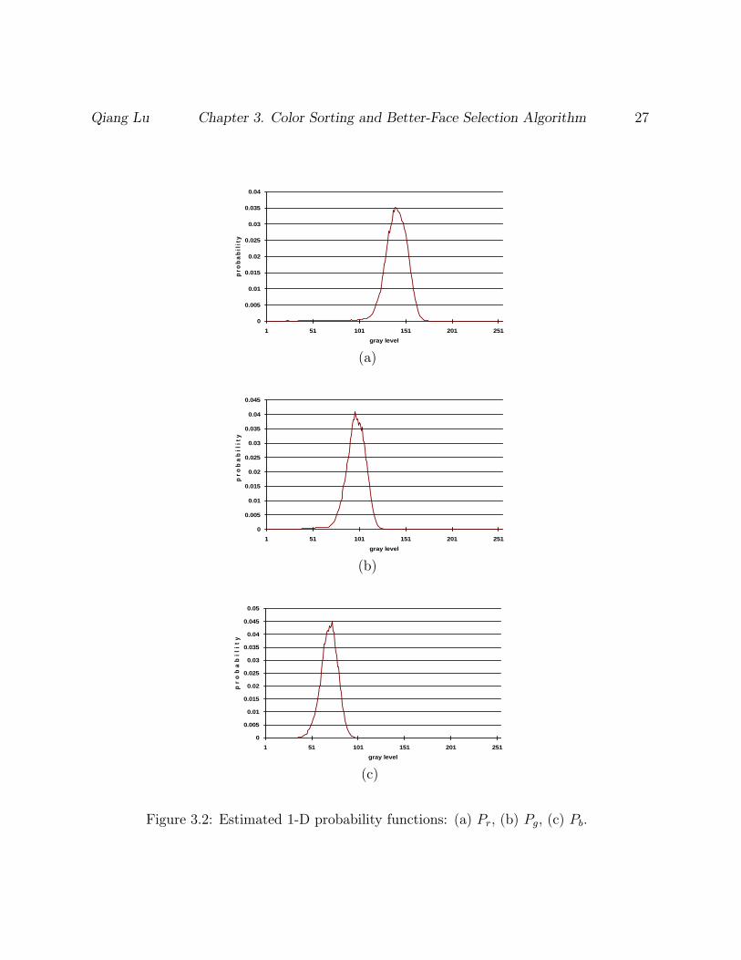
Another possible color representation is suggested in [4]. Instead of using a 3-D estimatedprobability function to present the color distribution of wooden parts, three 1-D probabilityfunctions each for one color channel were used. These three 1-D estimated probabilityfunctions are Pr = [pr(r)], Pg = [pg(g)], and Pb = [pb(b)] for red, green, blue color channels

respectively, and P = [Pr Pg Pb]T . Based on elementary probability theory, it should be

clear that

pr(r) =∑g

∑b

p(r, g, b) (3.8)

pg(g) =∑r

∑b

p(r, g, b) (3.9)

pb(b) =∑r

∑g

p(r, g, b) (3.10)

For wood part color image I, let the total number of pixels in this image be denotedby N . Let nr(r) denote the number of pixels with gray level r of the red color channel ofI, let ng(g) denote the number of pixels with gray level g of the green color channel of I,and let nb(b) denote the number of pixels with gray level b of the blue color channel of I.Pr, Pg, and Pb can be calculated as follows:


Pr = [pr(r)] =

[nr(r)

N

](3.11)

Pg = [pg(g)] =

[ng(g)

N

](3.12)

Pb = [pb(b)] =

[nb(b)

N

](3.13)

Figure 3.2 shows the three estimated 1-D probability functions computed for the samewooden panel part as was shown in the last section. Figure 3.2(a), 3.2(b), and 3.2(c) showthe distributions of Pr, Pg, and Pb respectively.

Let P1 = [P1r P1g P1b]T be the estimated probability functions computed from one

part face, and P2 = [P2r P2g P2b]T be the estimated probability functions computed from

another part face, then the color difference is computed as

d(P1, P2) = |P1 − P2|l1 = |P1r − P2r|l1 + |P1g − P2g|l1 + |P1b − P2b|l1=

∑r

|p1r(r)− p2r(r)|+∑g

|p1g(g)− p2g(g)|+∑b

|p1b(b)− p2b(b)| (3.14)

The methodologies for using this representation are basically the same as those used withestimated 3-D probability function method. Hence they will not be described here.

3.1.4 Average gray value method

Another possible color representation for wooden parts has been suggested by [103]. Insteadof probability functions, the color of a part surface is characterized by average gray levelsfrom three color channels. Thus the vector ~µ = (µr, µg, µb)

T , where µr, µg, and µb arethe average gray levels for red, green, and blue channels respectively, is used as the colorrepresentation. Let ~µ1 = (µ1r, µ1g, µ1b)

T be value computed from one part surface, and~µ2 = (µ2r, µ2g, µ2b)

T be value computed from another part surface, then the distance isdefined as

d( ~µ1, ~µ2) = |µ1r − µ2r|+ |µ1g − µ2g|+ |µ1b − µ2b| (3.15)


gray level

pro

ba

bil

ity

0

0.005

0.01

0.015

0.02

0.025

0.03

0.035

0.04

1 51 101 151 201 251

(a)

gray level

pro

ba

bil

ity

0

0.005

0.01

0.015

0.02

0.025

0.03

0.035

0.04

0.045

1 51 101 151 201 251

(b)

gray level

p

ro

ba

bil

ity

0

0.005

0.01

0.015

0.02

0.025

0.03

0.035

0.04

0.045

0.05

1 51 101 151 201 251

(c)

Figure 3.2: Estimated 1-D probability functions: (a) Pr, (b) Pg, (c) Pb.


Given this color representation, the methodologies for using it are very similar to that ofthe estimated 3-D probability function method and the estimated 1-D probability functionmethod, and hence will not be discussed here.

3.1.5 Test Results and Conclusions

Tests were conducted to determine the capabilities of each above representations. Thetest samples were 900 red oak parts supplied by a manufacturer of edge-blued panel parts.The 900 samples were grouped into two sets. The first set is consisted of 150 trainingsamples. The second set is consisted of 750 test samples. The 150 training sample werecarefully picked from the 900 samples to define the color classes to be used in the colorsorting. The sizes of each of the 900 test samples were all about the same ranging fromabout 10 to 12 inches in length, and about 2 to 21

2inches in width. All were 29

28inches thick.

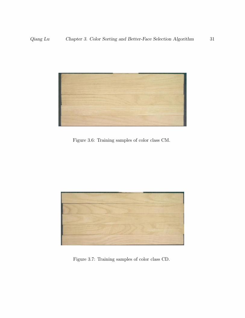
The 150 training samples were manually classified into six color classes. Those six colorclasses and an out class which are used for color classifications are shown in Table 3.1. Thissorting was done very carefully, putting only samples in a color class that everyone agreedbelonged to that class. There is no training samples for the out class since out is a catchallclass, parts not belonging to other classes are placed into the out class by default. ClassA is dark red as seen in Figure 3.3. Class B is red with some green as seen in Figure 3.4.Class CD is dark brown as seen in Figure 3.7. Class CL is light brown as seen in Figure3.5. Class CM is medium brown as seen in Figure 3.6. Class D is red with some white asseen in Figure 3.8.

The tests were performed in two steps. First, the 150 training samples used to definethe color class prototypes were scanned, and a prototype for each color class was computed.The training samples were then classified using real-time color sorting algorithm and thepercentage of correct classification was calculated. Second, the rest of the 750 sampleswere classified using the real-time color sorting algorithm. Samples classified into thesame color class were used to create panels. These panels were examined and put intothree categories: clear, acceptable, and unacceptable. This was the ultimate criteria forevaluating each representation. The manufacturer had set a goal for the automatic systemto generate at least 90% clear and acceptable panels.

The partial test results for the step 1 testing is shown in Table 3.2 for the estimated 3-D


Table 3.1: Color Class Definitions

Name Color Signature Number of samplesA dark red 25B red with some green 25CD dark brown 25CL light brown 25CM medium brown 25D red with some white 25Out all others none

Figure 3.3: Training samples of color class A.


Figure 3.4: Training samples of color class B.

Figure 3.5: Training samples of color class CL.


Figure 3.6: Training samples of color class CM.

Figure 3.7: Training samples of color class CD.


Table 3.2: Estimated 3-D Probability Function Method Partial Test Result

Class Sample A B CD CL CM D Min. Sorted asA 1 0.305 0.905 0.580 1.639 1.121 1.708 0.305 A

2 0.715 1.308 0.736 1.794 1.416 1.856 0.715 A3 0.430 0.641 0.780 1.493 0.966 1.565 0.430 A4 0.481 0.505 0.621 1.312 0.760 1.384 0.481 A5 0.364 0.825 0.774 1.586 1.118 1.654 0.364 A

B 1 1.191 0.662 1.052 0.670 0.621 0.743 0.621 CM2 0.862 0.289 0.797 1.198 0.558 1.259 0.289 B3 0.642 0.344 0.624 1.312 0.664 1.378 0.344 B4 0.871 0.302 0.705 1.122 0.458 1.194 0.302 B5 0.454 0.463 0.638 1.368 0.824 1.437 0.454 A

CD 1 0.537 0.976 0.457 1.640 1.068 1.713 0.457 CD2 0.721 1.110 0.527 1.611 1.175 1.671 0.527 CD3 0.743 1.240 0.640 1.763 1.339 1.822 0.640 CD4 0.731 0.432 0.493 1.248 0.531 1.318 0.432 B5 1.150 0.545 0.945 0.860 0.533 0.942 0.533 CM

CL 1 1.499 1.053 1.306 0.352 0.930 0.476 0.352 CL2 1.449 1.004 1.248 0.301 0.838 0.428 0.301 CL3 1.524 1.101 1.339 0.361 0.931 0.354 0.354 D4 1.725 1.356 1.530 0.407 1.167 0.421 0.407 CL5 1.450 1.054 1.252 0.314 0.871 0.382 0.314 CL

CM 1 1.295 0.824 1.013 0.615 0.477 0.653 0.477 CM2 1.287 0.726 1.080 0.644 0.521 0.692 0.521 CM3 0.822 0.576 0.703 1.345 0.661 1.405 0.576 B4 0.968 0.535 0.752 1.110 0.309 1.159 0.309 CM5 0.939 0.608 0.660 1.143 0.357 1.192 0.357 CM

D 1 1.574 1.205 1.382 0.364 1.019 0.334 0.334 D2 1.597 1.215 1.402 0.336 1.015 0.343 0.336 CL3 1.503 0.956 1.267 0.677 0.738 0.603 0.603 D4 1.728 1.391 1.591 0.606 1.277 0.537 0.537 D5 1.642 1.198 1.432 0.310 1.007 0.224 0.224 D


Table 3.3: Estimated 1-D Probability Function Method Partial Test Result

Class Sample A B CD CL CM D Min. Sorted asA 1 0.510 2.415 0.960 4.492 2.841 4.693 0.510 A

2 1.711 3.448 1.884 5.038 3.802 5.232 1.711 A3 0.998 1.361 1.223 3.889 1.825 4.076 0.998 A4 1.027 0.898 0.834 3.461 1.351 3.637 0.834 CD5 0.463 1.84 0.922 4.157 2.286 4.348 0.463 A

B 1 3.012 1.367 2.528 1.613 0.931 1.762 0.931 CM2 2.241 0.585 1.963 3.065 0.805 3.220 0.585 B3 1.456 0.664 1.350 3.381 1.114 3.554 0.664 B4 2.076 0.370 1.721 2.848 0.472 3.005 0.370 B5 1.070 0.986 0.998 3.549 1.452 3.724 0.986 B

CD 1 0.560 2.277 0.923 4.452 2.716 4.653 0.560 A2 1.067 2.812 1.243 4.501 3.182 4.701 1.067 A3 1.453 3.230 1.647 4.922 3.601 5.118 1.453 A4 1.407 0.525 1.167 3.233 1.003 3.400 0.525 B5 3.006 1.231 2.552 2.049 0.903 2.199 0.903 CM

CL 1 4.131 2.792 3.624 0.453 2.370 0.595 0.453 CL2 3.867 2.524 3.375 0.499 2.104 0.697 0.499 CL3 4.077 2.749 3.572 0.543 2.325 0.502 0.502 D4 4.690 3.545 4.239 0.782 3.137 0.705 0.705 D5 3.854 2.656 3.355 0.565 2.257 0.623 0.623 D

CM 1 3.105 1.523 2.624 1.388 1.075 1.534 1.075 CM2 3.222 1.519 2.759 1.588 1.050 1.729 1.050 CM3 1.655 0.826 1.562 3.489 1.231 3.656 0.826 B4 2.137 0.418 1.823 2.915 0.504 3.065 0.418 B5 1.929 0.571 1.565 2.968 0.616 3.126 0.571 B

D 1 4.251 3.121 3.778 0.557 2.726 0.483 0.483 D2 4.342 3.150 3.855 0.471 2.740 0.496 0.471 CL3 3.895 2.207 3.412 1.238 1.742 1.293 1.293 D4 4.794 3.701 4.322 1.102 3.295 0.900 0.900 D5 4.454 3.110 3.949 0.390 2.674 0.272 0.272 D


Figure 3.8: Training samples of color class D.

probability function and Table 3.3 for the estimated 1-D probability function. For each ta-ble, Column 1 shows color class which the sample part was originally classified as. Column2 shows the sample number. Column 3 to 8 show the color distances between a certainsample to the prototype of each color class. Column 9 shows the minimum distance andcolumn 10 shows the classification result. Compare to the partial result of Table 3.3, theestimated 3-D probability function representation showed significantly higher precision incolor classification those sample parts than the estimated 1-D probability function repre-sentation method. For Class A, the first 5 samples were all correctly classified by using3-D method while only 4 of them were right by using 1-D method. Though for ClassB only 3 of the 5 samples were correctly classified using 3-D method while 4 of themwere right using 1-D method, but for Class CD, CL, and CM, the number of correctlyclassified samples is significantly higher by using 3-D method than 1-D method. This istrue for Class D as well. The test results for the average gray level representation is notshown here because this method was incapable of color sorting any of the samples correctly.

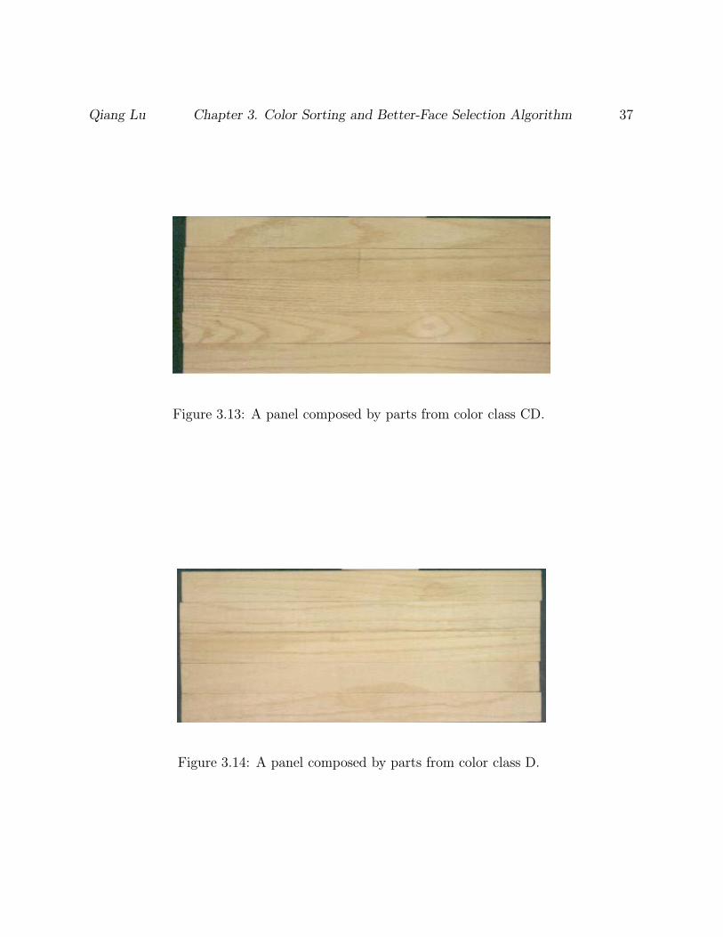
When testing on the rest of 750 samples using 3-D and 1-D representation methods,90% of the clear and acceptable panels are created by using the 3-D representation methodwhile only 30% of the clear and acceptable panels are created by using 1-D representationmethod. Figure 3.9 shows a clear panel composed by parts classified as Class A. Figure3.10 shows a clear panel composed by parts from Class B. Figure 3.11 shows a clear panelcomposed by parts from Class CL. Figure 3.12 shows a clear panel composed by parts fromClass CM. Figure 3.13 shows a clear panel composed by parts from Class CD. Figure 3.14shows a clear panel composed by parts from Class D.


Figure 3.9: A panel composed by parts from color class A.

Figure 3.10: A panel composed by parts from color class B.

The estimated 3-D probability function representation approach seems very mathemat-ically sound and produced the best sorting results, however, using it is relatively compu-tationally intensive and requires a good deal of memory as well. Consider a typical imagethat has 8 bits per color channel, each channel thus has 256 gray levels. The total numberof colors of the 3-D estimated probability function is 256 × 256 × 256, or 16,777,216. Toaddress this problem, a number of experiments were conducted. It was experimentallyshown that only the 6 most significant bits per color channel is needed to produce goodcolor sorting results. Thus the full color space for the estimated 3-D probability function isreduced to 64× 64× 64 elements, or 262,144. The color variations appearing in hardwoodpart make up only a small portion of this reduced full color space. Therefore the size ofthe estimated probability function can be further reduced to 11,000 elements. Using this


Figure 3.11: A panel composed by parts from color class CL.

Figure 3.12: A panel composed by parts from color class CM.


Figure 3.13: A panel composed by parts from color class CD.

Figure 3.14: A panel composed by parts from color class D.


Figure 3.15: Parts classified as out.

application specific information allows the computation intensity and memory demands tobe greatly reduced. It is felt that real-time color sorting is feasible by using this represen-tation under the assumptions just stated.

For the estimated 1-D probability function representation, consider a typical color imagecontaining 8 bits of information per color channel, each of these three estimated probabilityfunctions contains only 256 elements. Hence computational complexity of this represen-tation is greatly reduced over the 3-D representation. This representation also requiresmuch less memory. Unfortunately the 1-D representation is not sufficient to capture all theimportant color needed to sort wooden parts. Tests showed that the algorithm is incapableof separating dark brown red oak parts from dark red oak parts. This capability is criticalto manufacturers that fabricate edge-glued panels.

The average value representation is computationally the simplest of the three and re-quires the least memory. But the presentation is incapable of characterizing the extend ofcolor variations that are presented in a wood part. Tests show that this sorting algorithmis even incapable in classifying with very distinct color classes, e.g. white, brown, and pink.Therefore it is unlikely that this method can meet the exacting demands associated withcolor sorting edge-glued panel parts.

Since the estimated 3-D probably function representation yielded the best sorting resultand after the representation has been revised, to speed up the algorithm so that it could


be run in real-time, this representation was chosen for this color-sorting application.

3.2 Color Sorting Algorithms

3.2.1 Color sorting training algorithm

The training algorithm is used to teach the system to identify the color classes that are tobe used during the real-time sorting process. A training sample is one face of an edge-gluedpanel part. This face represents what is considered to be a prototypical example of thecolor class to which the face has been assigned.

The following is the training algorithm:

1. For the jth training sample of ωi, scan its image, and compute Pi,j.

2. Repeat step 1 until all images of training samples belong to ωi are processed. ComputePωi

and Ti.

3. Repeat step 1 and 2 until all color classes are processed.

Please note that though the threshold value Ti is computed from the scanning informa-tion, it can be manually altered during real-time sorting to meet the varying productiongoals of the plant. As the Ti gets smaller, the parts sorted into class ωi all have a moreuniform color, and the color characteristics of these parts are closer to the training samplesof ωi, and vice versa.

3.2.2 Real-time color sorting algorithm

The real-time algorithm actually performs the color sorting with parts moving throughthe system at the desired throughput rate. The following is the real-time color sortingalgorithm:

1. For a part surface, scan its image, compute Ps.


2. Compute d(Ps, Pωi), if d(Ps, Pωi

) < Ti, mark ωi, otherwise unmark it.

3. Repeat step 2 until all predefined color classes are compared.

4. If all classes are unmarked, label this part with “out”; otherwise label it with ωi, whereamong all the marked color classes, d(Ps, Pωi

) is the minimum.

3.3 Better-Face Selection Algorithm

Furniture panels, such as cabinet doors and table surfaces, always have two faces, but onlyone face is important, i.e., the door front and table top surface. The important face mustbe color matched, while the other need not be. The better-face selection algorithm is re-sponsible for selecting the better face of a wood part so that it can be used to create thevisible surface of the panel.

The real-time color sorting algorithm passes two pieces of information about each partface to the better-face selection algorithm. These are 1) the class label of the color classto which the face has been assigned, and 2) the face’s color distance value to the classprototype. Consumers like some colors of wood more than others, so each color class isassigned a priority based on management perception of consumer preferences. Assume fora part x, the color class labels of its faces are label1 and label2 and the distances are d1 andd2 for face 1 and face 2 respectively. The better face selection algorithm is as follows:

1. If color priority of label1 is greater than label2, face 1 is selected.

2. If color priority of label2 is greater than label1, face 2 is selected.

3. If color priority of label1 is the same as label2, then face 1 is selected if d1 < d2,otherwise face 2 is selected.

The information about the priority of each color class is stored on disk and can be changedby the operator using a utility program. Figure 3.16 shows a part’s face being selected byusing the better-face selection algorithm, and Figure 3.17 shows the face of the same partnot selected by the algorithm.


Figure 3.16: The side selected by Better-face selection algorithm.

Figure 3.17: The side not selected by Better-face selection algorithm.

3.4 Reducing computational complexity for real-time

sorting

To increase the throughput of the real-time sorting system, the computation complexitymust be greatly reduced. To achieve the goal − sorting 3.5 secs/part, the following modi-fications were made:

1. The scanning device collects image with 32 pixels/inch down board resolution and 75pixels/inch across board resolution. The color sorting algorithm only needs half thisresolution, i.e. 16 pixels/inch down board resolution and 38 pixels/inch across boardresolution. So the number of image pixels to be processed is reduced to 1

4th of the

original size.

2. Shading correction and histogram generation are only done to the image region con-taining wood part.

3. For the training sample set, only about 11, 000 colors occur in these images. It isreasonable to reduce the histogram array size to 11, 000 plus 1 entries. The 11, 000entries contain the frequency of color occurrence of these 11, 000 colors, and the extraentry contains the summation of frequency of color occurrence from all other colors.This not only saves computation time, but also the memory needed for storing thehistograms.


4. The current system scans a part first, then does the sorting calculation. It is possibleto sort wood parts while scanning. This requires extra programming effort which isbeyond the scope of study.

My work has only implemented the first three measures and the color sorting systemhas achieved a throughput of 5.6 seconds/part. I believe that if the last measurement isfully implemented, the throughput of the system can be expected to reach 3.5 seconds/part.

Chapter 4

System Hardware Overview

4.1 Introduction

The purpose of this chapter is to describe the hardware components of the prototype ma-chine vision system for color sorting edge-glued panel parts. The purpose of the prototypesystem is to establish that hardwood edge-glued panel parts can be automatically sortedand that the resulting sorted parts increases the number of high value panels created. Toestablish this proof-of-concept requires creating a hardware and software system that canbe tested in a manufacturing facility and that can be operated by plant employees. Thismeans that the hardware components must be designed to withstand the rigors of the in-dustrial environment,e.g., dust, temperature and humidity variations, and generally roughtreatment. It also means that the software system had to be designed so that the systemcould be easily be operated by plant personnel. To aid in evaluating the prototype, thesoftware system should be able to detect any hardware problems that could affect systemaccuracy. The desire to have the software detect operational problems with the hardwarewas based on the desire to determine whether failures in the hardware components wereresponsible for system performance problems or whether there was a basic problem withthe algorithms that were being employed. The software part of this prototype will be dis-cussed in Chapter 5.

Figure 4.1 shows the basic components of the prototype machine vision system. Thesystem can be broken down into a number of functional units:

1. a materials handling system for moving parts through the imaging components;

43

Qiang Lu Chapter 4. System Hardware Overview 44

AC light

controller

ultrasound sensor object detect

sensor

top camera white target

top carmera

camera

controller

converyer

roller roller

belt

fencefeed ojectfrom here

slave computer

High speed datatransfer interface

bottom camerawhite target

bottom camera

68HC11micro-controller

master computer

camera

controller

from COM 1

COM 1

parallelport connection

to data

transfer

interface

to camera

controller

master(slave) computer

inside look

board

COM 2

modem phone line

COM 2

phone line

modem

Figure 4.1: System diagram.


2. an image processing system for imaging and processing the digital image data of bothpart faces;

3. a control system for controlling overall system operation;

4. environmental enclosures for protecting the electronic and imaging devices from dust;

5. a remote dialup facility for providing a method to support the prototype from Blacks-burg.

Each of these functional units will be described in some detail later. This description willbe followed by a brief explanation of how the system operates in its typical real-time oper-ating mode.

Figure 4.2 shows the outward appearance of this system. The linescan cameras andlights are put inside the cabinets above and below the conveyor belt. In this figure, onlythe top cabinet can be seen clearly. Figure 4.3 shows this system from another view. Theconveyor belt now is on the right side of the photo. The big cabinet on the left side of thephoto is also an equipment cabinet. The two PCs, two modems, and a power supply areput inside this cabinet. The open window of this cabinet is for the PC monitor. On top ofthis cabinet are two signal lights, one is green and one is red.

4.2 Image Processing System

The image processing system on this prototype is fairly complex and is comprised of anumber of components. For purposes of this description, it is useful to subdivide this sys-tem into a number of operational components and then to describe the function of eachof these units. The components include the image processing computers, the cameras, theillumination sources, the interface for connecting the color cameras to the image processingcomputers, and a parallel port communications connection between the two computers fortransferring large amounts of data between computers quickly.


Figure 4.2: The outward appearance of the color sorting system. The linescan cameras andlights are put inside the cabinets right above and below the conveyor belt.


Figure 4.3: The outward appearance of the color sorting system from another view angle.The conveyor belt is now on the right side of the photo. The two PCs, two modems, anda power supply are put inside the cabinet shown on the left side of the photo. On top ofthe cabinet are two signal lights.


4.2.1 Image processing computers

Two image processing computers are used on the prototype, basically one computer forprocessing each part face. Two computers are used in order to increase throughput. Twocomputers can be used since the processing of a part face is not dependent on the process-ing of the other part face. The only communication required between the two computersoccurs at the end of the processing of the two part faces. One of the computers, the slave,must pass a small amount of information to the master so that the master can determinewhich part face is the better one to be used in manufacturing a panel. For modes of op-eration other than real-time processing, the communication between the two computersrequires more data to be transferred between machines. In such situations the master-slaverelationship greatly simplifies the task of writing the communications software.

Before proceeding, it is important to point out that the prototype machine vision sys-tem was developed incrementally. In the original configuration, it was capable of processingonly one part face. Once that capability was tested in a manufacturing facility, the systemwas modified to allow both part faces to be imaged. The master and slave computers arenot the same because the current slave was purchased first and was used in the initialconfiguration to image and process one part face. When the system was modified to allowboth part faces to be imaged and processed, the slave computer had been discontinued.Hence, a different, faster processor was selected and is used as the master.

The master computer on the prototype is an IBM PS/2 Microchannel bus 66 MHz486 DX2 personal computer with 16 megabytes of main memory running DOS. The mainmemory size is needed to store the color image data with the other information neededto do the analysis. Note that to achieve real-time operation everything must be memoryresonant. There is simply no time to go to disk to get information. The master has a VGAdisplay, a keyboard, and 500 megabytes of disk storage, which is needed in order to storeall the information needed to train the system, to store the training results, and, of course,to store the software system including diagnostic programs. At the beginning of real-timeoperation, necessary information is transferred from disk to main memory where it staysmemory resonant until real-time operation is stopped.

The master computer runs all the man-machine interface software. Commands to thisinterface are entered via the master’s keyboard, and the menu selections are displayed onthe master’s display. The master is responsible for not only the man-machine interfacebut also for processing color imagery from the bottom part face and for making the final


decision as to which part face is the better one to use in manufacturing a panel. The mas-ter computer analyzes the bottom part face on the prototype because the top and bottomcameras have to be offset from one another. A part reaches the bottom camera’s field ofview and leaves the bottom camera’s field of view later than it does the top camera. Hence,the faster computer is used to analyze this imagery.

The slave computer is controlled by commands sent through a serial communicationsport from the master computer. This serial communications channel connects the masterto the control computer and the control computer to the slave machine. (The control com-puter is a Motorola MC68HC11E2 micro-controller and its function will be described laterin this chapter.) Communications among these machines are bidirectional with informationpassing from the master to the slave via the control computer and from the slave to themaster via the control computer in a similar manner.

The slave computing unit is an IBM PS/2 Microchannel bus 50 MHz 486 DX2 personalcomputer with 16 megabytes of main memory and 500 megabytes of disk storage runningDOS. The memory and disk space requirements for the slave are almost the same as forthe master’s. The slave computer does not have a keyboard or a display. All commandsit executes are sent to it by the master over the serial communications line. The slavecomputer is responsible for collecting and analyzing the color image data of the top partface. The face color class label and a small amount of other data are sent to the masterover this same serial channel.

Note that while the control computer is responsible for managing a number of systemwarning and informational lights, commands to initiate these control functions come fromeither the master or slave computers via this same serial link.

There is also a bidirectional parallel port connection that directly links the master andslave computers so that large data files can be transferred in a timely manner. For example,if an operator wants to see a color image of the top face of a part, an image that is collectedby the slave computer, he must see this image on the master computer’s display since itis the only one available. The parallel port connection provides the mechanism for imagedata to be transferred from the slave to the master.

Regarding the display of color image data, it is important to note that a VGA monitorwill display only 256 colors, far fewer colors than exist in even a very uniform red oak part.


To get high quality displays of color images on a VGA display a special display program isused. This display program allocates the 256 colors to the most frequent colors appearingon a part’s face [75].

Both the master and slave computers have a serial communication port connection toa high speed modem which in turn is connected to a phone line (one phone line for eachcomputer). This hookup allows immediate troubleshooting of hardware and software prob-lems and facilitates upgrading software. It also provides a very convenient mechanism forpersonnel at Virginia Tech to monitor the system as it is operating.

The two computers scan their respective part faces independently and use the samealgorithm to arrive at the color class label for the face each is required to process. Oncethe slave computer has completed its analysis, it sends its classification of the top partface and a small amount of other information through the serial communication port backto the master computer. Simultaneously, the master is generating its classification for thebottom part face. Using a better-face strategy, the master chooses either the top or bottompart as the better face. The better-face selection algorithm uses classification results andother information obtained by the slave computer to make its decision. After the better-face selection algorithm is executed, the master sends the better face result to the controlcomputer so that these results can be displayed on the informational lights, which tell plantpersonnel the results of the automatic analysis.

4.2.2 Parallel Port Communication

As stated previously the prototype machine vision system uses two image processing com-puters. The man-machine interface that controls the prototype is located on the mastercomputer. The only monitor and the only keyboard available on the prototype are con-nected to the master computer. Whenever an operator wants to see information collectedby the slave computer, this information must first be transferred to the master and thendisplayed on the master’s monitor. There are at least three situations where the amount ofdata that must be transferred is quite large. One of these situations is when an operatorwants to see an image of the top part face, the face collected by the slave computer. Inthis instance, the entire image file must be transferred, a file that can contain a number ofmegabytes of data. In such circumstances, using a serial port for communicating large datasets would impose a substantial delay in executing a command, so a parallel port connec-tion between the master and slave was provided. This communications connection is used


to transfer image data of parts (a transfer from the slave to the master), to transfer imagedata of a white target used to check lighting conditions for the top part face (a transferfrom the slave to the master), and to transfer threshold data (a transfer from the masterto the slave). The last two types of data will be described in greater detail in Chapter 4.

A standard parallel communication pin specification [94] is used to connect the twocomputers together. The exact pin specification used is shown in Figure 4.4. The pinspecification is provided in Table 4.1. Using this standard parallel communication pinspecification [94], five bits can be sent simultaneously through data lines D0 to D4, anddata can be transmitted in both directions simultaneously because the connections arecrossed. The protocol needs to use a strobe signal line to keep track of the data transferpace. The BUSY bit is employed for this job and is connected to D4 on the other parallelport.

The following specify the communications protocol at the byte level. Since the parallelport can transfer only 4 bits at a time, a byte is split into the lower four bits and the higherfour bits.

1. The sending computer begins the data transfer with the lower four bits. It writes thesebits to data lines D0 - D3 and sets the value of D4 to 0 so that the receiving computerwill get a value of 1 at its BUSY pin.

2. The receiving computer waits for the value of the BUSY bit to change to 1. It thenwrites the lower four bits it just received back onto data lines D0 - D3 to return themto the sending computer for error checking. To indicate that it has placed the lowerfour bits it just received back onto D0 - D3, bit D4 is set to 0 so that the sendingcomputer’s BUSY bit will change to 1.

3. The sending computer waits for its BUSY bit to change to 1. It then stores thereturned lower four bits. Note that the sending computer stores these four bits becausethe error checking is done at the byte level. The sending computer then writes thehigher four bits to the data lines and sets D4 to 1. This changes the value of thereceiving computer’s BUSY bit to 0.

4. This time, the receiving computer waits for the BUSY bit to change its value to 0.The received high four bits are again returned to the sending computer on lines D0 -D3, and the computer also sets data bit D4 to 1. The sending computer will then geta value of 0 for its BUSY bit.

5. At this point the communication is complete. The sending computer reassembles the


o o o o o o o o o o o o o

o o o o o o o o o o o o

o o

12345678910111213

141516171819202122232425

o o o o o o o o o o o o o

o o o o o o o o o o o o

o o12345678910111213

141516171819202122232425

Figure 4.4: Parallel port communication pin specifications.


Table 4.1: Parallel Port Pin Specifications

Pin Number Signal Name Meaning1 ∼STROBE Indicates data transfer2 D0 Data line - bit 03 D1 Data line - bit 14 D2 Data line - bit 25 D3 Data line - bit 36 D4 Data line - bit 47 D5 Data line - bit 58 D6 Data line - bit 69 D7 Data line - bit 710 ∼ACK Last character received11 ∼BUSY Printer busy12 PE Printer has no paper13 SLCT Printer is on-line14 ∼AUTO FEED Automatic CR after LF15 ∼ERROR Data transfer error16 ∼INIT Reset printer17 SLCT IN Turn printer on-line

18-25 GND Ground


byte from the two nibbles it has just received and checks the data byte returned fromthe receiving computer to make sure it is the same as the data byte as in the originalfile.

Besides the byte transfer issue, there are still time-out interrupt and manual interruptproblems. A time-out interrupt occurs whenever the sending computer or the receivingcomputer does not respond in a fixed amount of time. The time-out interrupt can begenerated by calling the IBM PC ROM (Read Only Memory) BIOS (Basic Input andOutput System) program. A manual interrupt occurs whenever the operator decides toterminate the data transfer for any of the following reasons: the transfer link is broken, orthe machine behaves abnormally. Pressing the escape key(ESC) will inform the computerof this interrupt. The interrupt will then stop the sending or receiving process and makethe process exit to DOS.

4.2.3 Color line-scan camera

The dimensions of parts used to make edge-glued panels vary depending on the productbeing manufactured. They may vary in length, width, and thickness. Since the goal of thiswork is to achieve an automatic analysis system that can run at near commercially usefulspeeds, consideration must be given to minimizing the amount of data that is collected.An effective way to do this is to use line-scan cameras. By incorporating a simple objectdetection device, the line-scan camera can be turned on just prior to a part entering its fieldof view and turned off just after a part leaves its field of view. Hence, one can minimize thenumber of rows of image data collected. By incorporating a width sensor for determiningpart width, one can also collect information from those adjacent sensing elements on theline that are actually imaging the part and not background. In this way, the number ofcolumns of image data that need to be analyized can also be minimized. For these reasons,a line-scan camera was chosen for use on the prototype.

The particular line-scan camera used is a Pulnix model TL-2600RGB. Figure 4.5 showsthis camera inside the camera and lights cabinet. Figure 4.6 shows the camera controller.This camera is a Charge Coupled Device (CCD) imager that contains a linear array of CCDcells. This linear array consists of 864 full color pixels per line, i.e. every pixel locationcontains three silicon elements. Each of the three is sensitive to either red, green, or bluecolor. Therefore, totally 864× 3 bytes must be transferred to get one complete line of colorimage data.


Figure 4.5: A closer view of the linescan camera and the fiber optic bundle used to conductlights to the scanning part’s surface.


Figure 4.6: The linescan camera controller.


This particular camera was selected because it is one of the few color line-scan camerason the market at the time the prototype was developed. Other color line-scan camerashave even higher resolution than this one. Since the widest part that needs to be imaged isonly 6 inches wide, this camera provides more than enough resolution for edge-glued panelpart inspection. Note that the spatial resolution being used on the prototype is 32 pixelsper inch. The motivation for a spatial resolution this high does not come from the colorsorting problem discussed here but from development work to be conducted on the proto-type after the color sorting work is completed. This development work involves locatingand measuring the spatial distribution of mineral streak on parts and incorporating grainmatching capabilities for finger jointing applications.

As with any photon counting device, a quantity of charge collects on the individualcells over a period of time defined as the integration period. The accumulated charge isproportional to the number of photons incident on the collection surface during the inte-gration period. Chosing the correct integration time is dependent upon the application.Short integration times minimize image blur as the part moves under the camera but some-times increase image noise because of quanta effects. This is particularly true in low lightlevels. Getting good quality images with short integration times requires a good deal oflight. Longer integration times increase image blur but reduce the amount of light needed.Experimentation is used to arrive at an acceptable compromise. On the prototype, theintegration period is set to approximately 1.7 millisecond. This rather long integrationtime helps reduce both image noise and the amount of light needed (this, as will be seenlater, helps reduce system maintenance) while not causing unacceptable image blurring.

This Pulnix camera uses a 35 millimeter camera format, i.e., the line of sensing ele-ments is precisely 35 millimeters long, and the imaging plane is located in exactly the sameposition from the lens mount as in a 35 millimeter camera. This format allows very highquality yet fairly inexpensive 35 millimeter camera lenses to be used. The lenses used onthe prototype are Nikkor which are of high quality and widely available. A 60 millimetercamera lens was selected for the prototype.

The silicon CCD sensor elements are more sensitive to longer wavelength light, i.e., theelements are more sensitive in the red part of the color spectrum and have a maximum inthe near infrared region. Because of this variation in sensitivity a number of optical filtersare used on the prototype, one of which is a cold infrared cutoff filter. This filter basicallycuts off all infrared light having wavelength longer than approximately 700 nanometers.This filter is part of the camera assembly provided by Pulnix. Since silicon is more sensi-tive to red, i.e., wavelengths in the 600 to 700 nanometer range, than green (500 to 600


nanometers) and is much more sensitive to green than blue (400 to 500 nanometers), twoadditional blue filters are used. These filters help even out the sensitivity of the sensingelements across the visual spectrum by reducing the amounts of red and green light thatcan enter the camera. Note these filters not only balance the sensitivity of the sensingelements but also markedly reduce the total amount of light reaching the imaging area.Hence, more intense illumination is required to get high quality images.

4.2.4 Direct memory access image acquisition interface

Both the master and slave computers have a Microchannel input and output data bus. Thetwo Pulnix color line-scan cameras are connected to the computers via a high speed, directmemory access Microchannel bus master interface board that was designed and built hereat Virginia Tech by Dr. Thomas H. Drayer [24] as shown in Figure 4.7. There is one ofthese interface boards in each of the two computers. The functioning of this interface canbe programmed through a computer’s I/O port. The highest transfer speed this board willsupport is about 3.5 Mbytes/sec. This interface board precisely controls when image datacollection is started and stopped. It also controls the field of view of the imagery collectedby controlling the range of pixels on any given line that is transferred to the computer.Large volumes of image data are transferred through this board to Microchannel bus andthen from the Microchannel to into a software controllable area of main memory.

The parameters used to control the functioning of this interface include the startingpixel number on the line-scan camera, i.e., the first element of each row of image data andthe number of pixels to appear in each row of image data. Note that these two parametersprovide control over the field of view of the camera, i.e., the number and placement of thecolumns of image data. Another control parameter is the number of color channels to becollected. For purposes of this prototype this parameter is always set to three so that allthree color channels can be collected.

Yet another control parameter is the maximum number of rows to be collected. Thevalue of this parameter depends on the amount of memory available on the host computersystem. It tells the board the maximum number of rows that can be collected before theallotted memory area for the image data will overflow. The address of the allotted memoryarea is another control parameter that must be pasted to the board. As the board beginsto collect data, it writes to the main memory beginning at this address. If the interfaceis not signaled to stop data collection before the specified maximum number of lines have


Figure 4.7: The high speed data transfer interface board, designed by Dr. Thomas H.Drayer.


been scanned, the board will automatically cease data collection and interrupt the hostcomputer, i.e., the master or the slave. If this problem occurs on the slave, it will signalthe master computer alerting it of the problem encountered.

The final control parameters are bits that signal the board to begin data collection andstop data collection. These bits allow one to begin image data collection very shortly beforea part enters a camera’s field of view and halt data collect just after the part leaves thecamera’s field of view.

As noted above, being able to control the field of view and starting and stopping datacollection at the appropriate times can markedly reduce the amount of data that must beanalyzed.

4.2.5 Illumination sources

The illuminants should be adjustable and provide uniform distributed light intensity alongthe line being scanned. One way to achieve such a goal is to use fiber optic light sources,which consist of a bundle of optic fibers. One end of the bundle points toward an illumi-nation source, e.g., a light bulb. The light from this source passes through the bundle andcomes out of the other end. At the other end of the bundle the ends of the fibers lie in astraight line with the ends pointing in the same direction. Since all the fibers are pointingin the same direction, the line of fibers illuminates a linear region. With an appropriatediffusing filter between the bulb and the end of the bundle where the light enters, very uni-form lines of light can be created. Figure 4.8 shows a light source. Figure 4.9 shows threelight sources are placed inside the camera and lights cabinet. Fiber optic bundles connectlight sources to the lights distributor shown at the bottom right conner of the photo.

The important factors concerning the light intensity provided are the wattage of thebulb providing the illumination and the length of the line of fiber ends. Given that thebulb wattage is fixed, the way to adjust the light intensity is to adjust the length of theline formed by the fiber ends. To increase the light intensity, one can use multiple lightbulbs with the corresponding number of bundles of optical fibers.

The fiber optic light sources used in the prototype are from the Fostec Company. These


Figure 4.8: The light source.


Figure 4.9: Inside view of the cabinet. Three lights sources (white boxes) are placed insidethe cabinet, each is connected to a fiber optic bundle. The linescan camera is placed onthe right side of the cabinet. Cooling fans can be seen placed on the cabinet door. The airconditioner is placed at the back of the cabinet.


sources use a 150 watt tungsten halogen bulbs. To inspect both upper and lower faces ofa part simultaneously, six fiber optic sources are used. Four sources, two per part face, areused for the surface illumination. The remaining two sources are used to illuminate theblue background seen by each camera. Using the background light sources provides a clearboundary between the board and background without causing concerns about shadows.

Another concern for using the fiber optic light sources is the dirty environment typicallyfound in wood product manufacturing facilities. The camera and the set of lights are placedin an enclosure. The use of fiber optic light sources allows this enclosure to be more or lesspermanently sealed. The bulbs can remain on the inside of the unit with the fiber opticcables carrying the light out to the object surface.

Tungsten halogen (T-H) light bulbs were chosen to be used as the light sources. Theywere chosen because T-H family bulbs have good color temperatures and are relativelyinexpensive. Unfortunately, T-H bulbs do not have a very flat spectral response across therange from 400 nanometers to 700 nanometers. Initial experiments clearly showed thatwhen T- H bulbs were used in conjunction with the Pulnix camera, poor quality colorimages were produced. To correct for the lack of a flat spectral curve across the 400 to700 nanometer range, filters are used in front of the camera. These filters provide a meansfor obtaining good imagery from the imaging system, but the use of these filters takes ahigh cost on the light budget of the system. The amount of light reaching the camera wentdown by a factor of eight when the filters were inserted in front of the lens.

There were three types of T-H bulbs considered to be used in the system: EKE, EJA,and DDL. Among these types of bulbs, EJA produces the most illumination, and DDLproduces the least. But the lifetime expectancy of DDL bulb is about one thousand hours,while the EKE lasts only about one hundred hours, and the EJA lasts only about 40 hours.The DDL bulb is the cheapest of the three. These characteristics of DDL bulb make itparticularly good when used an industrial machine. Thus the DDL bulb was chosen to beused in this system.

There were a number of problems that needed to be addressed before DDL bulb couldbe used in the prototype machine. The illumination supplied by DDL bulb is the leastamong the three bulb types of the T-H family. To increase the illumination, the lightinggeometry was adjusted. The end of each fiber optic bundle for which the light comes outwas moved closer to the part face. The iris adjustment where the bulb light comes out ofthe light source was opened to its maximum extent. Finally the DDL bulbs run at a higher


voltage than the other bulbs would have been so that it will produce more illumination.

To make the illuminant stay at a constant level, a special DC power supply is used. Theoutput voltage of the power supply can either be adjusted manually or through a computercontrollable interface. If the illuminant changes, it can be adjusted to previous level bychanging the output voltage of the power supply either manually or under computer con-trol. On the prototype machine, the lights are continuously monitored and the computeradjusts the output voltage of the power supplies to correct any lighting variation that mayoccur.

4.3 Sensing, Controlling, and Communicating

4.3.1 Overview

The system’s control computer is used to collect data from sensors, control lights, controlwhite targets, and control communication between the master and the slave computers.It frees the master and slave computers from having to perform peripheral jobs. Hence itimproves the overall performance of the system. Figure 4.1 shows the circuit connectionsbetween MC68HC11E2 and all the sensors, lights, white targets, and communication ports.

There are two sensors used in the system: an infrared object detection sensor and anultrasonic width measurement sensor. The infrared sensor is responsible for detecting thepresence of a part. Monitoring it allows the prototype to know when a part will enter thefield of view of each of the two cameras. The width sensor measures the width of the part.This information is used to reduce the number of rows and columns of image data thatneed be collected.

There are two types of lights that need to be controlled. The first type is the lightsources that illuminate the part faces. The light intensity striking each part face mustbe accurately controlled. The second type is the informational lights. These are eitherswitched on or off and provide the operators information about the system status and in-formation about processing results.


A white target is used by the system to collect shading correction information to checkfor the variations of lighting. The white target can either be extended to cover the entirefield of view of the camera or be retracted into its storage area. Note that even when it isfully retracted, part of the white target’s surface is still visible to the camera. The reasonfor this is that it allows the target to be used for checking light intensities as parts arebeing processed by the system.

The master computer must be able to send commands to the slave, and the slave mustbe able to send its better-face information back to the master. This communication is donethrough each PC’s serial communication port.

4.3.2 Control computer

The control computer used in the prototype is a Motorola MC68HC11E2 micro-controller.It has 512 bytes of electrically erasable programmable ROM (EEPROM) and 256 bytes ofrandom access memory (RAM). The EEPROM is used to store the control program. TheRAM is used to store commands from one of the PCs, data from the sensors, and someintermediate results generated by the control program.

There is an analog-to-digital (A/D) converter on the micro-controller chip. The A/Dconverter converts 0 to +5 volt analog signal to 8-bit binary data. The converter is con-nected to the analog output of the ultrasonic sensor. It is used to collect part widthinformation.

Five 8-bit addressable input/output (I/O) ports are build-in on chip. Extra circuitswere built to extend the addressable I/O ports to ten. Two ports are used for inputs andeight ports are used for outputs. Port 0 is an output port used for outputting control valuesto 8 informational lights. Port 1 is an input port used for inputting the object detectionsensor value. Port 2 is an output port used for outputting control values to signal lightsand white targets. Port 3 is an input port used for inputting the values obtained from theultrasonic width measuring sensor. Port 4 to 9 are output ports used for output controlvalues to the six light sources, each port is used to control one light source.

There is only one RS232 communication port on this micro-controller chip. Both


computers’ communication port #1 (COM1) are connected to this micro-controller portthrough a multiplexing circuit. Two computers can read values off RS232 port simultane-ously, but can not write to this port at the same time. Commands send by one computerwill be buffered by on-chip memory and after the end of command string is received, themicro-controller sends this string to the other computer.

There are three basic types of commands that the master or the slave computers cansend to the control computer. These commands are: read data from a sensor, write datato control a device, and transfer data between the master and the slave computers. Thethree types of commands cover the three tasks the control computer performs.

4.3.3 Sensors

To read data from a sensor, either the master or slave PC sends a command to theMC68HC11E2 using character strings in the following sequence: a special ASCII char-acter (a smilley face), followed by command READ, and the address of the sensor. Theoutput signal from that sensor is immediately latched into the MC68HC11E2’s buffer, andthe data is transferred back to the requesting computer through the communication port.

The infrared sensor used in this system is the SA LR41887, it is also called MINI-BEAM.It is a product of the Electronics Corporation. As illustrated in Figure 4.10, the infraredsensor is composed of two parts: an emitter and a receiver. In Figure 4.11 the emitter isthe device fixed inside the metal case on the left of the conveyor belt nearer to the reader.The receiver is the device fixed on the metal fence of the right side of the conveyor belt.Properly aligned, the infrared beam generated by the emitter will hit the photo diode ofthe receiver. The photo diode is sensitive to infrared light. It behaves as a switch, and isalways off, i.e., a 0 volt signal, until turned on by an infrared beam, i.e., a +5 volt signal.The source side of the photo diode is connected to a +5 volt power supply, the sink side ishooked up to a digital input port of the MC68HC11E2. When no object is in the beam, thephoto diode is turned on by the infrared beam and the input port of the control computerreceives a +5 volt signal from the sensor. When an object is in the beam, the photo diodereceives no infrared light, thus it is turned off. The input port of MC68HC11E2 receivesa 0 volt signal. In a TTL digital circuit, +5 volts denotes binary one, and 0 volts denotesbinary zero. In other words, a binary signal 1 means no object is in the beam, and binary0 means an object is in the beam.


fenceobject

+5V

to 68HC11

infra-red light bult

infra-red sensorinfra-red light path

object moving direction

Figure 4.10: Infrared object detect sensor.


Figure 4.11: Infrared and ultrasonic sensors are placed by the sides of the conveyor belt.


As seen in Figure 4.1, an object being scanned first passes through the infrared sensor,then the ultrasonic sensor, then the top camera, and finally the bottom camera. Sincethe conveyor belt runs at a constant speed, the time between when the front edge of theobject reaches the infrared sensor and when it reaches other points along the conveyorcan be easily calculated. The belt runs at 2 feet/second. The distance from the infraredsensor to the ultrasonic sensor is 0.5 feet, which translates to a 0.25 second delay. The topcamera is 1 feet away from the infrared sensor. This translates to a 0.5 second delay. Thebottom camera is 2 feet away from the infrared sensor. This translates to a 1 second delay.The delay information is used by the scanning program to precisely start and stop imageacquisition.

The ultrasonic sensor used in the prototype system is a product of the Simens Company.As shown in Figure 4.12, it is composed of three parts: an ultrasonic wave generator, areceiver, and a control unit. In Figure 4.11, the wave generator and receiver can be seenfixed inside a metal case on the left side of the running belt further from the reader. Theprinciple of its operation is simple. At time 0, the source transmits an ultrasonic wave. Thiswave bounces off any object that is in the wave’s path. A receiver receives the reflectedwave at time ∆t. The timing difference ∆t is converted to an electronic signal by thecontrol unit. The larger ∆t is, the higher the voltage that is output by the control unit.Since sound travels at a constant speed, the distance is proportional to the time elapsed.Thus it is also proportional to the output signal voltage. The voltage range of this signal isbetween 0 to +5 volt. The A/D converter of MC68HC11E2 converts an analog signal thatis between 0 to +5 volt to binary value that range from 0 to 255, i.e., binary 0 correspondsto a 0 volt analog signal and binary 255 corresponds to +5 volt. Through experimentation,the mapping between the binary number and the distance from the transmitter and theobject can be calculated. Denote the distance traveled by the wave as r, and the binaryvalue as b, thus

r = b · f (inches) (4.1)

where f is the factor that converts the binary data to a corresponding distance value.

As we stated earlier, the part being scanned is always a rectangular parallelepiped. Thefence against the conveyor belt is parallel to the direction the belt is running. The operatoris required to feed a part into the prototype by placing it against the fence. This makessure that a side of the part is always next to the fence and will always be parallel to the


fence

object

ultra-sonic wave generator

control unit

to 68HC11 board

r0

r 1

accoustic receiver object moving direction

ultra-sound wave

Figure 4.12: The ultrasonic sensor.


fence. Thus the width measured by the sensor at any position along the part will alwaysbe approximately the same.

To measure a part’s width, two parameters must be known: r0, the distance from thesensor to the fence; and r1, the distance from the sensor to the side of the part nearest tothe sensor. The width w can be calculated by

w = r1 − r0 = f(b1 − b0) (inches) (4.2)

where the binary value, b1, is the read from the ultrasonic sensor when no object is present,and where b0 is the value read from the sensor when a part passes by.

Knowing the length and width of a part, the computer will begin image acquisition justprior to a part entering the field-of-view of a camera, will terminate image data collectionjust after the part leaves the field-of-view of a camera, and will collect a minimum numberof columns of image data. The wider the part the more columns that need be collectedand vice versa.

4.3.4 Lights and white targets

To control a device, the PC sends a command to MC68HC11E2 using character strings inthe following sequence: a special ASCII character (a smilley face), followed by the WRITEcommand, the address of the device, and the control value. The devices that can be con-trolled in this manner include the six DC light sources, eleven AC informational lights, andthe two white targets.

The six DC lights are separated into two groups, three lights per group. In Figure 4.9,one group of lights are shown. For each light group, two are used to illuminate a face ofthe part, the third one is used to illuminate the background.

A light source has three parts: a DDL bulb, an iris that controls the amount of lightthat can enter the fiber optic bundle, and a power supply. To vary the light intensity, theoutput voltage of the power supply can either be manually adjusted or adjusted through


computer control. Since the system is designed to automatically adjust the amount oflight generated by each light source, computer control is used. Each power supply has ananalog input interface, and the output voltage can vary from 0− 20 volts according to theanalog input value. The control computer sends an 8-bit binary value through one of itsI/O ports to a Digital-Analog Converter (DAC), and this DAC converts this digital valueto an analog signal used as an input to a power supply’s analog control.

There are total eleven AC lights: two signal lights and nine informational lights. Thesignal lights include a red light and a green light as shown in Figure 4.3 on top of thedevice cabinet. When the red light is on, the system is either scanning a part or processingdata. The operator should not place another part on the conveyor belt while this light is on.When the green light is on, the system is free and is waiting for another part to be fed into it.

The nine informational lights are labeled A, B, C, D, E, F, OUT, UP, and DOWN asseen in Figure 4.13. The first seven lights are used to display the label assigned to a partby the system, and the last two are used to display the better-face selection result, i.e.,whether the better face is the top part face of the bottom part face.

Each of the AC lights is connected to a triac. Each triac is connected to an optoisolator.Each optoisolator is connected to to one bit of an I/O port on the micro-controller. Anoptoisolator is a device that prevents feedback AC current from damaging digital circuits.A triac is an electronic gate turned on and off by changing the current direction of a controlsignal. The control signal used here is +5 volts (TTL standard), and the AC signal beingcontrolled is 120 volt. When the I/O port control bit is set to 0, the triac is deactivated,and a light is turned off. When this bit is set to 1, the triac is activated, and the light isturned on.

There are two movable white targets on the prototype system, one is for the top cam-era and one is for the bottom camera. Each white target has two positions: retractedand extended. When the white target is retracted, the camera sees a small portion of thewhite target, and any part that might be on the conveyor belt. When the white target isextended, the camera sees only the white target.

The white target is attached to a pneumatogenic piston. This piston has two air inputports, one at each of its ends. Applying air to either end drives the piston to the other end.The white target can be extended or retracted depending on the end of the piston where


Figure 4.13: The informational lights used to display color sorting results.


the air is applied. A solenoid is used to change the direction of the air flow. The inputof the solenoid is 120 volt AC. By turning a control signal on or off determines which endof the piston air is applied. The switch is connected to a triac. The triac is connected toan optoisolator. And finally the optoisolator is connected to one bit of an I/O port of themicro-controller. The white target is extended when bit is set to 0, and is retracted whenbit is set to 1.

4.3.5 Serial communication

If the string send by a PC to the MC68HC11 is not started with a smilley face, the stringwill be directly transferred to the other PC regardless of its contents. This allows the mastercomputer to send processing commands to the slave computer, and to receive better-faceinformation from the slave computer.

4.4 Remote Debugging Auxiliary Facilities

The prototype machine was taken to a manufacturering plant over 200 miles from Blacks-burg for testing. To troubleshoot system problems and to upgrade the system softwaredirectly and conveniently from Blacksburg, a remote dialup system was included on theprototype.

The master and slave computers used in prototype system at the plant are consideredas the host computers for remote dial-up purposes. The two PCs used for dialup in Blacks-burg are thus considered to be as the remote computers. Point-to-Point Protocol (ppp) isused for establishing the communication between a remote PC and a host PC.

A remote computer does not need to be very powerful since it is only used to monitor anddisplay what is happening on the host computer. All the real computation is done by thehost machine. Since the scanned images are frequently being checked by displaying themon computer monitors, each remote computer in Blacksburg is equipped with a moderateresolution monitor. The remote computers are two IBM PCModel 30 running DOS. For theModel 30, the CPU is Intel 80286. The monitor is VGA. The host and the remote computersare each connected to a 14,400 bps external modem through its serial communication port.


The modem is hooked to an analog phone line. Remote PC A is used to dial up the mastercomputer. Remote PC B is used to dial up the slave computer. Figure 4.14 illustrates theprotocol setup.

analog phone line

modemremote PC host PCmodem

from COM1 from COM2

Figure 4.14: The illustration of Point-to-Point Protocol.

The software used for ppp is PC Anywhere, a product of Symtex Corporation. Thissoftware is part of the Norton Utilities package. PC Anywhere has two sets of programs,one set supports the host, the other set supports the remote. It allows the remote com-puter to dial-up the host through the phone line. After the connection is established, theremote computer has the ability to control all software residing on the host computer. Alsothe screen displays on the remote machine are the same as the displays on the host. Thehost computer accepts keyboard strokes from not only its keyboard, but also characterssent to it by the remote. While the operator can control the host computer, people at theremote site can monitor system status and can operate the scanning system as well as theoperator. Any warning messages appearing on the host’s computer screen are displayed on


the remote computer’s monitor as well.

PC Anywhere supports a talk function. When the talk function is activated, the softwarebrings up a window on each computer. The upper half of this window is for the operator totype in words. The lower half is for displaying messages typed by operator at the other endof the communication line. This function is very useful especially for system troubleshoot-ing. Besides talk, PC Anywhere also supports file transfers. This allows one to upload newversions of the color sorting software to the host computer from the remote machine, and todownload data from the host to the remote machine for analysis by personnel in Blacksburg.

Chapter 5

The System Software

5.1 System Software Overview

There are three types of operations that the software system must support: system setupand light control, system training, and real-time color sorting. The purpose of the systemsetup and light control software is help in the setup of the scanning hardware system sothat the best possible images can be obtained. The purpose of the system training softwareis to control training data collection, to create the color class prototypes, and to establishthe color class thresholds. The purpose of the real-time color sorting software is controlthe color-sorting of wood parts. Besides these three basic types of operation, the softwaresystem must also provide some general utilities, e.g., the display of scanned images. Alsosince the color sorting system was to be placed in a manufacturing plant and operated byplant personnel, the software system had to provide a user friendly interface.

The following three sections discuss the design of the user interface, the system setupand light control software, and the system training software and the color sorting software.

5.2 User Interface

The user interface uses a menu tree structure. Figure 5.1 shows the menu tree for theprototype system. When the machine is turned on, the screen of the master computer

77

Qiang Lu Chapter 5. The System Software 78

immediately switches to the Main Menu page. There are three entries on the Main Menupage. The entries include System Setup for setting up the lights or other parts of themachine, Color Sorting for either training the system or to do real-time color sorting, andGeneral Utilities for performing such operations as: scanning a part or displaying an image.

Main Menu

1. System Setup

2. Color sorting

3. General Utilities

2. Initialize the foreground light.

System Setup Menu

Parameter Setting Menu

2. Set better-face priority values

1. Adjust threshold value for a color group

General Utility Menu

1. Scan a part

2. Display an image

3. Setup Password

3. Real-time color sorting

2. System training

1. Color sorting parameter set

Color Sorting Menu

2. Generate class histograms and threshold value

1. Scan training sample parts

System Training Menu

3. Generate confusion matrix

3. Initialize the background light.

4. Collect shading correction information

5. Check foreground light

6. Check background light.

1. Adjust camera height, focus, and pointing angle.

Figure 5.1: The graphic user interface menu tree designed for the prototype machine.

When any of these entries are selected, a new menu page pops up. When the SystemSetup is selected, a menu titled System Setup Menu is popped up. The four entries allowone to set up either the camera or the lights, or to collect shading correction information.The Color Sorting Menu is popped up when the Color Sorting entry of the Main Menu is


selected. The three entries on the Color Sorting Menu allow one to set the sorting param-eters, train the system, or do color sorting. The General Utility Menu contains entries toscan a part, display an image, and set up a password.

To display the machine status and/or the processing results in a user friendly way, twomethods are employed: a Graphic User Interface (GUI) that is displayed on the mastercomputer’s monitor and some informational lights that can easily be seen by an operatorwho is removing parts from the system and putting them in the appropriate class bin.

5.3 System Setup and Light Control

System setup and light control functions include the following actions: camera height andpointing angle adjustment, camera focusing, light pointing and intensity adjustment, shad-ing correction data collection, and light intensity checking. These four functions correspondto the four entries of the System Setup Menu as shown in Figure 5.1.

Note that all these setup operators are performed with the material handling subsystem,i.e., the conveyor belt, turned off. It is important that one remembers this when readingthe following subsections that describe each of the setup procedurers.

The color sorting algorithm is extremely sensitive to the quality of the color imagescollected. Things that can effect the color image quality include camera settings and lightsource settings. Note, the color sorting algorithm is particularly sensitive to variations inlight intensity.

The hardware for scanning one part face is shown in Figure 5.2. This hardware in-cludes a linescan camera, a camera controller, a high speed data transfer interface (notshown here), and a host computer. The illumination devices include three light sources,three fiber optic cables, a MC68HC11E2 control computer, and the host computer. Toautomatically perform shading correction, a white reference target is needed. The whitetarget can be extended into the linescan camera’s field of view by a pneumatogenic sys-tem. In the extended position, the white target is used to collect shading correction data.Obviously, to do either system training or real-time color sorting, the white target must bein its retracted position. Even in its retracted position, the white target occupies some of


pis ton

white targetis retracted

white targetis extended

optic fiber

linescan camera

camera controller

to high speeddata transfer

interface

MC68HC11control computer

light source

light source

light source

host

computer

pneumatogenic

camera view

To COM 1

Figure 5.2: Hardware used for scanning one part face.


the color camera’s field of view. The reason for this is so that the white target can be usedto check for any variations in lighting that may occur. During both training and real-timecolor sorting, the system continuously checks the white target image data to determinewhether any variations in lighting are occurring.

5.3.1 System setup functions

In order for the system to collect the best possible image data, the system should be setup using the procedure described below:

1. Adjust the camera’s height to change the field of view.

2. Adjust the camera’s pointing angle.

3. Initialize the background light if needed.

4. Adjust the camera’s focus.

5. Initialize the foreground lights.

6. Collect shading correction information.

7. Collect run-time light checking information.

One good way of adjusting the camera and the light is to scan an image, and checkthe response of the linescan camera. The image data should be collected and processed asfollows:

1. Collect K lines of white target color image data. Let Rk = [rk(i)], Gk = [gk(i)], andBk = [bk(i)] denote the red, green, and blue components of the kth line collected,where 1 ≤ k ≤ K.

2. Compute the average response for each pixel in each channel of data, i.e., compute

scanred(i) =K∑k=1

rk(i)/K (5.1)

scangreen(i) =K∑k=1

gk(i)/K (5.2)

scanblue(i) =K∑k=1

bk(i)/K (5.3)


where by convention SCANred = [scanred(i)], SCANgreen = [scangreen(i)], and SCANblue =[scanblue(i)]. This averaging helps reduce the effect of thermal noise.

This data reflects the current status of the camera and lighting conditions. To makethis data easy to use, a GUI page is used. This GUI page is shown in Figure 5.3. TheGUI page displays slightly different information depending on what action the operator istrying to perform. However the same basic format is always used. The title specifies thefunction the operator is currently performing. The words following the title explain thesteps an operator should follow to perform function he is attempting. The legends describethe information being displayed inside the frame. The solid lines are previously recordeddataWHITEred, WHITEgreen, andWHITEblue of the extended white target. The procedureto collect those data is discussed in Section 5.3.2. The dashed lines are the current dataSCANred, SCANgreen, and SCANblue collected from the extended white target. The GUIpage outputs red, green, and blue colors to display lines to show the red, green, and blueoutput from the color camera respectively. In this figure, the six lines displayed are hardto separate. However the top two lines are from the red channel, the middle two lines arefrom the green channel, and the bottom two lines are from the blue channel.

The horizontal axis represents the pixel position. The vertical axis represents the pixelgray level. The horizontal axis ranges from 1 to 864 corresponding to the 864 pixels ofthe linescan camera. The vertical axis ranges from 0 to 255 corresponding to the 256 graylevels possible in each color channel.

The six light sources are separated into two groups: lights for the top camera, and lightsfor the bottom camera. The three lights in one group are named as TOP1, TOP2, andBOTTOM, where TOP1 and TOP2 are the lights used to illuminate the part’s surface,and the BOTTOM light is used to illuminate the blue background. The title of the GUIpage indicates which light source group is the one currently being controlled. The upperleft corner of the page displays the current control value that is being sent to the indicatedlight by the micro-controller.

The upper right corner of the GUI page contains a small circle labeled “OVER”. Thisis used to indicate if any pixel element in a scan line is saturated. A pixel is saturated ifits value is equal to 255 in any of the color channels. The output from the camera cannever be greater than 255 since an 8 bit A/D converter is used. If a pixel is saturatedthe information provided from that picture location will be distorted. When no saturationoccurs, the interior of the circle is black. When saturation occurs, the interior of the circle


Figure 5.3: A GUI page used for camera and lighting controls.


is displayed as red.

To adjust the camera’s pointing angle, height, and focus, Entry 1 of the System SetupMenu is used. To initialize the foreground light, Entry 2 of the System Setup Menu isused. To initialize the background light, Entry 3 of the System Setup Menu is used. Tocollect shading correction information and run-time light checking information, Entry 4 ofthe System Setup Menu is used. To check the foreground lights before any part scanningis performed, Entry 5 of the System Setup Menu is used. To check the background lightsbefore any part scanning is performed, Entry 6 of the System Setup Menu is used. Therun-time light checking is embedded into the scanning program, and is performed whenevera part is being scanned.

Light and camera adjustment is performed on only one imaging system at a time, i.e.,on either the top face imaging system or the bottom face imaging system. Thus beforeentering the System Setup Menu Page, the operator must choose which scanning system hewants to perform the adjustment on. Once this selection is made, the GUI page posts thescanning system currently being examined as a reminder to the operator. The followingdiscussion is all based on adjusting the top surface scanning system. The principles andprocedures used on the top scanning system is exactly the same as that would be used onthe bottom scanning system.

Camera height and pointing angle adjustment

To set the camera height, only SCANred is displayed inside the frame of the GUI page.SCANred was selected because to perform those functions, only one channel of data needsto be considered and because silicon based color cameras are always more sensitive to redlight. Finally a part is inserted into the camera’s field of view. This part is placed againstthe fence and appears in the same position as it would if were being carried through thesystem by the conveyor belt. Note that part should be of the same width as the widestpart the system will have to inspect. The widest possible part is 7 inches.

The camera height is directly related to the width of the field of view. The higherthe camera, the wider the field of view and the lower the across board resolution, and viceversa. By watching the change of the displayed line while adjusting the camera’s height, thefield-of-view of the camera can be easily adjusted to cover the widest part to be scanned.


At least a portion of the white target must be in the field of view of the camera in order forrun-time light checking to be performed. Note that as the camera is moved up and downthe focusing of the lens may have to be adjusted. The adjustment need only keep the part“roughly” in focus.

To set the camera pointing angle, only SCANblue is displayed inside the frame of theGUI page. SCANblue was selected because the camera pointing angle is adjusted using theblue background. First the background light is adjusted so that it is as close as possibleto the reflective blue target with one end of the fiber optic cable being the same distancefrom the target as the other end. The camera pointing angle should be adjusted so that ithas approximately uniform lighting across the field of view by the blue background.

Light pointing and intensity adjustment

The foreground lights should be set so that the full gray level resolution is being used forpart scanning without saturating the camera. To initialize the foreground lights, SCANred

is displayed in the frame of the GUI page. The white target is moved to its extendedposition. The white target is supposed to represent the brightest parts to be scanned. Thedisplayed line reflects the light response from the white target. The red color channel of thelinescan camera is the most sensitive to the light provided by the bulbs. The foregroundlight pointing direction and intensity should be adjusted such that the red channel has themaximum response to the white target without saturating any pixel in the linescan camera.This corresponds to the situation where the displayed line approaches the top frame linewithout the OVER indicator being filled with red.

The lights can be adjusted through the following methods:

1. Adjust the fiber optics to change the shape of line SCANred.

2. Adjust the iris of the light sources to increase or decrease the intensity of the lightoutputs.

3. Adjust the voltage output of the foreground lights. Make sure that each foregroundlight source outputs approximately the same amount of light.

It should be noted that the second method is used to make major changes in intensity andthe third method is used to make small changes. The value sent to the DAC to control the


lighting is displayed on the upper left corner of the GUI page. By pressing the up arrowkey “↑” or down arrow key “↓”, the values send to the DAC can be either increased ordecreased. To switch control to the other foreground light, the TAB key is used. Once theadjustment is finished, the checking program can be exited by pressing the ESCape key.This will cause the System Setup Menu to appear.

The procedure to initialize the background light is similar to the foreground light ini-tialization. However SCANblue is displayed instead of the SCANred. The white target isput in the retracted position. The blue background should be adjusted so that it will notappear too bright but should have a value that will simplify background extraction.

Camera focusing

First put a piece of white paper with black lines on the white target which is in extendedposition. By adjusting the camera focus, the contrast between the black lines and back-ground changes. Once the lines have maximum contrast from white background and pixelson a line all have approximately the same value, the camera focus is properly adjusted.

5.3.2 Shading correction data collection

The purpose of shading correction is to remove nonuniformities in lighting and sensitivityof sensing elements across a camera’s field of view [86].

The selection of white reference target used for shading correction is very important.The reference target should be chosen according to the following criteria: First, the re-flectance of the reference target should be close to the reflectance of the brightest possiblepart to be scanned. Obviously it should be somewhat lighter than the brightest possiblepart. Thus the lights can be adjusted using this target to produce images that fully usethe dynamic range of the camera gray levels without saturating the camera. Second, thereflection of the reference target should be uniform across its surface. This makes adjustingthe camera and lights easier. This uniformity is also crucial for image shading correction.Third, the reflective spectral characteristics of the reference target should not deteriorateovertime. Thus a plastic white target with about 75% reflectance was chosen as the refer-ence target. The plastic target can be easily cleaned with soap and water. Because it is


very cheap, if it is damaged or cannot be appropriately cleaned for any reason, it can beeasily replaced.

To perform shading correction on an image, certain data must be collected prior toapplying the shading correction algorithm. After the lights have been properly adjusted,the shading information can be collected. The data that must be collected and the initialprocessing steps that must be applied to these data are as follows:

1. Put the lens cap on the camera lens to prevent any light from entering the camera.Collect K lines of image data. Let Rk = [rk(i)], Gk = [gk(i)], and Bk = [bk(i)] denotethe red, green, and blue components of the kth line collected where 1 ≤ k ≤ K.


blackred(i) =K∑k=1

rk(i)/K (5.4)

blackgreen(i) =K∑k=1

gk(i)/K (5.5)

blackblue(i) =K∑k=1

bk(i)/K (5.6)

where by convention BLACKred = [blackred(i)], BLACKgreen = [blackgreen(i)], andBLACKblue = [blackblue(i)]. This averaging helps reduce the effect of thermal noiseon the information that will be used to do the shading correction.

3. Send the white target to its extended position to cover the camera’s field of view.Remove the lens cap and scan K lines of color image data off the white target whoseface lies in the same plane as a part face would be during the scanning of a part.Let Rk = [rk(i)], Gk = [gk(i)], and Bk = [bk(i)] denote the red, green, and bluecomponents of the kth line collected where 1 ≤ k ≤ K.


whitered(i) =K∑k=1

rk(i)/K (5.7)

whitegreen(i) =K∑k=1

gk(i)/K (5.8)

whiteblue(i) =K∑k=1

bk(i)/K (5.9)


where by convention WHITEred = [whitered(i)], WHITEgreen = [whitegreen(i)], andWHITEblue = [whiteblue(i)]. Again the averaging is used to reduce the effect of noiseon the data that will be used in the actual shading correction process.

The data collected from steps 1 and 2 are used to measure dark current effects on thelinescan camera. The dark current effects are the none-zero gray level outputs from thecamera when no light enters the camera body. The dark current reflects the characteristicsof the camera CCD sensor cells. The data collected from step 3 and 4 are used to measurethe brightest response from the white target. This response defines the dynamic range inintensity with which the camera must cope. The data collected is used to measure nonuni-formities in lighting and/or sensitivity of the CCD sensing elements.

Once the dark current data and white target data have been collected and processed,shading correction can be applied to color imagery as it is being collected. The procedureis described as follows:

1. Collect a line of digital color imagery from a color line scan camera. Let R = [r(i)],G = [g(i)], and B = [b(i)] denote the red, green, and blue components of this line ofdata.

2. For each element i of this line of data, compute

rcorrected(i) =255× (r(i)− blackred(i))

whitered(i)− blackred(i)(5.10)

gcorrected(i) =255× (g(i)− blackred(i))


bcorrected(i) =255× (b(i)− blackred(i))


The data Rcorrected = [rcorrected(i)], Gcorrected = [gcorrected(i)], and Bcorrected = [bcorrected(i)]represent the red, green, and blue components of the shading corrected line of colordata.

5.3.3 Light intensity checking

The lights must be controlled so that they output a constant level of illumination. Thelights must be checked after start up but prior to any system image collection. The lights


are also checked immediately after any new part is scanned. This light checking is calledrun-time light checking.

Light checking data collection

The data WHITEred, WHITEgreen, and WHITEblue collected for shading correction are alsoused as the reference data to check and adjust the lights during system setup. Another setof data that must be collected along with the shading correction information is the referencedata used for run-time light checking and background light checking. The run-time lightchecking includes both the checking of foreground light and background light. This datamust be collected and processed as follows:

1. Put the white target into its retracted position. In this position the camera can seea small portion of the white target, but the majority portion of the camera’s field ofview is the blue background. Scan K lines of color image data off the white targetwhose face lies in the same plane as a part face would be during scanning of thepart. Let Rk = [rk(i)], Gk = [gk(i)], and Bk = [bk(i)] denote the red, green, and bluecomponents of the kth line collected where 1 ≤ k ≤ K.


runtimered(i) =K∑k=1

rk(i)/K (5.13)

runtimegreen(i) =K∑k=1

gk(i)/K (5.14)

runtimeblue(i) =K∑k=1

bk(i)/K (5.15)

where by convention RUNTIMEred = [runtimered(i)], RUNTIMEgreen = [runtimegreen(i)],and RUNTIMEblue = [runtimeblue(i)]. Again the averaging is used to reduce the effectof noise on the data.

The white target part of the data supplies information about the foreground lights. Theblue background part supplies information about the background light. For color sorting,the backgrounds lights have been turned off because of mechanical problem and it is notcrucially needed for color sorting application. But if the system is used to detect holes,stain or mineral streaks, the background lights have to be turned on in order to separate


the backgrounds from the part. For completeness sake, the background light checking isdiscussed here.

Light intensity checking

To check foreground lighting, the white target is put into the extended position, andSCANred and WHITEred are displayed. The line of WHITEred is the reference line. Theline of SCANred reflects the current lighting situation. The following is the procedure usedfor making foreground light adjustments:

1. Display the GUI page with the line of WHITEred.

2. Send out white target to the extended position.

3. Collect image data and process the data to acquire SCANred.

4. If the difference between SCANred and WHITEred is less than a threshold value Tlight,then quit this GUI page and return to the System Setup Menu with information indi-cating a successful light adjustment. The difference value dlight is computed using

dlight =∑i

|scanred(i)− whitered(i)| (5.16)

5. Update the line of SCANred.

6. If ESCape key is hit, then quit this page and return to the System Setup Menu pagewith information showing the lights have not been properly adjusted.

7. If UP (or DOWN) arrow key is hit, then increase (or decrease) the control value andsend it to the output voltage of the power supply currently active.

8. If TAB key is hit, then switch the lights that are active.

9. Repeat from step 3.

Once the light is properly adjusted, the GUI page will quit automatically and the SystemSetup Menu page will be displayed along with a message that indicates that the lightinghas successfully been adjusted.

The checking procedure for the background light is similar to the checking procedurefor foreground lights except that the lines displayed are SCANblue and RUNTIMEblue. This


is because the background target is blue. When the lights hit the target, the lights reflectedinto the camera is mostly blue.

Run-time light intensity checking

The foreground and background lights are automatically checked after each part is scanned.After the part passes out of view of the linescan camera, the camera can only see theblue/black background and part of the white target. A number of lines of image data arecollected to compute SCANred and SCANblue. If the lighting difference dlight is greater thana threshold value Tlight, the lighting conditions must have changed while the previous partwas being scanned. Since this change would most probably have caused the part face to beassigned to the wrong color class, the operator is notified via a message on the computerscreen to retrieve the part and adjust the lights. Otherwise, the scanning system continuesits normal scanning procedure. The value dlight can be calculated using

dlight =∑i

|scanred(i)− runtimered(i)|+∑i

|scanblue(i)− runtimeblue(i)| (5.17)

If a light bulb is changed, the operator should go back to the System Setup Menu page,use Entry 5 or Entry 6 to adjust the foreground or background lights.

It should be noted, that the color sorting quality is closely related to the lighting con-dition of the prototype machine. If after intensive adjustment, the system lights can notapproach the original lighting condition set of the machine, the color sorting system shouldbe trained again using the new lighting conditions.

5.4 Color Sorting

In this section, two activities are discussed in detail: system training and real-time colorsorting. Entry 2 of the Color Sorting Menu is used to do system training. Once entered,the System Training Menu is popped up. Entry 3 of the Color Sorting Menu is used for


real-time color sorting. Entry 1 of the Color Sorting Menu is to set the threshold valuesand better-face value.

5.4.1 System training

The System Training Menu page has three entries. Entry 1 is for training sample scan-ning. Entry 2 is to compute the class prototype estimated 3-D probability functions andthe threshold information needed for color sorting. Entry 3 is for computing the trainingresults, i.e., classify the training samples by applying the information just computed, andproduce a confusion matrix to show how well the classification results are.

To implement the color-sorting training algorithm, the operator must input the numberof color classes to be used, the name for each color class, which informational lights are tobe used to denote each color class, and the number of training samples for each color class.The training samples then can be scanned one at a time. The image file of each sample isproperly named and stored to disk for later use. Assume the 8th training sample of colorclass B is just scanned, the image file for this sample is named as B8.img by convention.

A GUI page as shown in Figure 5.4 is used to help the operator keep track of how thetraining is proceeding. This GUI page can be brought up by entering Entry 1 on the Sys-tem Training Menu page. Column 1 on this GUI page gives the color class names. Column2 and 4 display the number of training samples available for each color class. Column 3and 5 display the number of samples that have been scanned. Column 2 and 3 are for thetop camera scanning system. Column 4 and 5 are for the bottom camera scanning system.Column 6 and 7 show which informational lights will be used to signify each color class.The informational lights are shown in Figure 4.13. Each row of the table corresponds tothe color class specified by the class name in column 1.

The cursor (a dark gray small square in Figure 5.4) can be moved to different cells. Thehelp information displayed at the bottom of the table explains to the operator as to whatactions he is supposed to take with regard to this particular cell. By moving the cursorto any place in the top row, one can modify the number of color classes that are to beconsidered. By moving the cursor to a name column cell, one can modify the label usedfor a color class. By moving the cursor to any cell in column 2 or 4, one can modify thenumber of training samples that the system expects to be scanned for that color class. Bymoving the cursor to a cell in column 6 or 7, one can modify which informational lights


Name Number of Samples

Top Camera (6 Classes)

Samples Scanned Number of Samples Samples Scanned

15 8 15 15 AA

B 15 15 15 15 B

CL 15 0 C

Light Mapping

#1 #2

CM 15 15 0 C

CD 15 0 15 C A

D 1515 0 D

10 B

D15 15

0

0

Use +/- to increase/decrease the number of samples to be scanned.

Bottom Camera (6 Classes)

Figure 5.4: A GUI page used for training sample scanning.


will be used to indicate that color class. Once all the required information has been input,the training sample data collection can be begun.

To start training sample data collection, one moves the cursor to a cell in column 3 orcolumn 5, and hits enter. Then the GUI page is switched to the scanning-in-progress page.The top surface will be scanned if the cursor is in column 3, otherwise the bottom surfacewill be scanned. The samples color class is indicated by the name given in column 1 in thisrow. Once scanning is finished for one color class or the scanning is interrupted manuallyby the operator, the scanning-in-progress page is switched back to the GUI scanning page.

Because the images scanned using the bottom surface scanning system are stored in themaster computer, and the images scanned using the top surface scanning system are storedin the slave computer, the names of stored images can be the same for the same sample onboth computers without causing confusion.

The scanning-in-progress page mostly displays information useful for program debug-ging. The only useful information for an operator is the name of the sample image to bestored. An operator can hit the ESCape key to interrupt this scanning process and returnto the GUI scanning page.

The basic part scanning procedure executed by the computer is as follows:

1. Turn on the green light instructing the operator to feed a part into the system.

2. When the part hits the object detect sensor, turn the red light on.

3. Measure the width of the part, and set the parameters for scanning.

4. Scan the part.

5. After scanning the part, do run-time light checking.

6. If the light has changed, then discard the scanned image, and quit the scanning pro-gram by notifying the operator the lights have changed. Otherwise save the image withthe given name.

7. Repeat from step 1.

After all the scanning samples have been scanned, the operator can use Entry 2 ofthe System Training Menu to generate class prototype estimated probability functions and


threshold values. The calculated threshold values can be modified using Entry 1 of Param-eter Setting Menu. The better-face priority value for each color class can be set by Entry2 of Parameter Setting Menu.

5.4.2 Real-time color sorting

The real-time color sorting is fully automatic. The operation is started when one selectsEntry 3 of the Color Sorting Menu. When the feed light is red, the operator waits anddoes not feed a part into the system. When the light turns green, the operator placesa part on to the system conveyor belt. Once the machine starts scanning, the feed lightturns to red again. The sorting results are displayed using informational lights on the sys-tem’s color sorting results panel. After the results are displayed the feed light turns greenagain. The operator reads the color-sorting and better-face selection results off the resultspanel, and places the processed part into the right bin with the part’s better face facing up.

The following describes the computer procedure for real-time color sorting:

1. Reset lights: turn the red feed light on, the green feed light off. Turn all informationallights off on the color sorting results panel. (master)

2. Initialize the system: load shading correction information− BLACKred, BLACKgreen,BLACKblue; WHITEred, WHITEgreen, WHITEblue. load run-time light checking infor-mation − RUNTIMEred, RUNTIMEgreen, RUNTIMEblue. load color class histogramsHi, i = 1, 2, . . . , L. load color class threshold values Ti, i = 1, 2, . . . , L. (master andslave)

3. Load better-face class priority values. (master)

4. Check lighting conditions. If it is significantly changed, quit scanning and inform theoperator to adjust the lights. (master and slave)

5. Turn green feed light on and the red off to instruct the operator to feed a part. (masteronly)

6. After a part moves past the object detecting sensor, start measuring the width andlength of the part. (master and slave)

7. Set up parameters for scanning using the width information just collected, and turnthe red feed light on and the green feed off. (master and slave)

8. Collect image data for both sides of the part. (master and slave)


9. Once the image data has been collected, compute classification results for both sidesof the part. (master and slave)

10. The top face classification result is transferred from the slave computer to the mastercomputer. (slave)

11. Select the better face using the better-face selection algorithm. (master)

12. Display the color sorting and better-face selection result by using the informationallights. (master)

13. Turn off red feed light and turn on green feed light.

14. Wait for the next part to move past the object detecting sensor and go to step 4.

Please note that some of the steps are performed by both the master and slave com-puters, while others are performed by the master computer only. The computers used toperform each step is indicated above.

Chapter 6

System Performance Testing

6.1 Introduction

The prototype color-sorting machine is designed to meet the needs of furniture manufac-turers. Hence, the quality of sorting by this machine must be better than that done byhumans, and the throughput must be higher. This is the only way manufacturers canjustify the purchase of such a device.

To fully demonstrate its capabilities, the prototype was designed to be industrially ro-bust. This means the machine must work reliably for long periods of time. It means thatthe machine will not fail in the very hostile environment of the plant floor. It also meansthat the sorting quality must be consistently high throughout production. And finally itmeans the machine must be easy for a plant personnel to operate.

Two types of testing were conducted on the prototype. The preliminary testing wasconducted to verify the capability of the color-sorting algorithm. It was conducted in thelaboratory. In-plant testing was performed in order to get experience in real-world plantoperation. The goals for the in-plant testing were to demonstrate the machine sorting ca-pabilities and its reliability. In this test, throughput was not particularly important, sinceit was believed that the desired throughput rate could be achieved once sorting quality wasverified. An unstated goal was to gain the experience necessary to improve the prototypemachine to achieve the desired level of industrial robustness.

97

Qiang Lu Chapter 6. System Performance Testing 98

6.2 Preliminary Testing

The preliminary testing was conducted at Brooks Forest Products Research Center at Vir-ginia Tech. This facility is air conditioned, and is maintained at a constant temperatureof approximately 72◦F. The air is relatively clean. The electricity power to the BrooksCenter is supplied by the Virginia Tech power plant. The variations in AC voltage arebelow 2%. The 900 samples used for the preliminary testing were carefully picked by thefurniture manufacturer. The prototype machine color sorted the 900 samples and approxi-mately 90% of the panels created from the sorted parts were clear or acceptable. This gavea clear indication that estimated 3-D probability function method is able to capture all thecolor information needed to color-sort panel parts for furniture manufacturing. Finally, allthe components of prototype color sorting system functioned as expected, at least, in thislaboratory type of environment. During the preliminary testing, the lights were well undercontrol, and the parts could be run continuously through the system for color sorting. Theminor problems that were encountered in the preliminary testing were easily solved.

6.3 In-plant Testing

6.3.1 Problems encountered

The prototype machine was then moved to the furniture manufacturer’s plant for in-planttesting. When the prototype was moved in, it failed immediately on almost every aspectof its operation. The training samples and training color classes were the same as thoseused in the preliminary testing. However, the parts to be color sorted were parts comingfrom the plant’s regular production. Compared to the selected 900 samples used in thepreliminary testing, the surfaces of the parts were not always free of mineral streak, and thecolor variations were significantly more pronounced than that encountered in the original900 samples. To record the statistical results, the sorted parts were counted by loads. Aload typically has 900 to 1000 parts. The machine sometimes sorted loads of parts so thatas high as 70% of the panels produced were clear or acceptable. However, sometimes thisfigure of merit went as low as 30%.

The machine could not be operated reliably over long periods of time. The plant wasvery dusty. The white target used to calibrate the lights would get extremely dirty afteronly a half-day’s operation. Also the camera lenses would get covered with dust as well.


When the white targets got dusty and the camera lenses got dirty, the light checking pro-gram would give a false alarm indicating the lighting conditions were bad.

The plant was not air conditioned. In the summer, plant temperature would go as highas 110◦F. In the winter, plant temperature would go as low as 40◦F. The plant temperaturedirectly affected the temperature of the light source power supplies. Each of these powersupplies has a sensor that indicates when its operational temperature gets too high. Insuch situations, the power supplies would automatically turn themselves off so that thelight source could cool down. When a light power supply shuts down, the light checkingprogram senses that a significant light change has occurred and stops any further imagescanning. When this happens, the machine’s operation is brought to a halt and stays sountil the light that went off automatically turns itself on again. This annoying situationoccurred most frequently during the summer, because of the hot temperatures in the plant.The four foreground lights were continuously turning themselves off and on. It was almostimpossible to continue operating the system under these circumstances.

Half of the electricity power used in the furniture plant is generated by the plant’s ownelectricity generator. The quality of the electrical power provided is very poor. AC voltagevariation can be as high as 30%. As was stated in Chapter 4, the intensity of lights changeswith the voltage supplied to the bulbs. Such a large variation made precisely controllingthe lights very difficult.

Besides the hostile environment, plant personnel posed yet another problem. The userinterface of the initial system was not well structured. It provided few hints to guide the op-erator on how to use this machine. Operators were always puzzled as to what actions theyshould perform. Operators had difficulty in scanning training samples, adjusting lights,and collecting shading data. There were too many entries in each menu page and theseentries were not properly named.

The training information should not be modified after the prototype histograms andcolor class thresholds have been generated. On several occasions, the operator made awrong entry and modified crucial training values. Obviously, whenever such an incidenthappened, system performance was adversely affected, usually disastrously so.

When collecting shading data, the white target should be at the same height as theparts that are to be scanned. However, during two days of testing, the operators were


feeding parts into the system that had different heights without re-collecting the shadingdata or re-training the system. Most of the parts fed into the system that were of a differentheight than the parts used to train the system and, consequently, at a different height thanthe white target, were sorted into the out class.

6.3.2 Making the prototype machine industrially robust

To improve the overall machine performance on the plant floor, a number of measures weretaken. These included modifying both the system hardware and software. The key toaccurately color sorting parts is to precisely control the amount of light produced by lightsources. To do this, fans were placed on the doors of the enclosures to increase the aircirculation inside these encloses. The goal was to keep the light source power supplies coolenough so that they would not automatically shut themselves off.

Second, the white target that was originally used on system was made of a very expen-sive material. The price of material was so high, it could not be regularly replaced evenwhen dust could no longer be removed from its surface. A plastic paper like white targetwas substituted for the expensive material. This plastic material could be cleaned usingsoap and water. If it got dirty, it could be inexpensively replaced. Operators were askedto clean the white target after every four hours of prototype operation. The purpose of thecleaning was to avoid the false alarms generated by the light checking system. The colorcamera lenses were also cleaned after every four hours of system operation.

Third, a new much more stable power supply was incorporated into the system. Itwas used to provide electrical power to the light sources as well as other components of thesorting system. Since it was much more stable than the multiple power supplies it replaced,the illumination level provided by the light sources was much more uniform over time.

After these measures were taken, the light sources became much more stable, and on hotsummer days, the frequency with which the light sources automatically turned themselvesoff was reduced to once per hour. Since the scanning system was cleaned very frequently,the scanned image quality was much more controlled and was of similar quality as thatachieved in the laboratory. Consequently, the average clear and acceptable panels producedper load reached the range from 72% to 99%, up from the previous rate of 30% to 70%. Theaverage clear and acceptable panels produced by an employee is only about 75%. Though


on average the system could perform better than a human, the manufacturer still wantedthis machine to be improved. The further improvements in the system will be discussed inthe next section.

The software was modified to be more user friendly and better organized. The GraphicsUser Interface (GUI) entries were reorganized to reflect the functionality of the system. Thename of each entry was modified to better reflect its function. When making any softwareparameter changes, a help menu is given to explain this change to the operator and to in-struct the operator how to perform this change in a step-by-step manner. Each of the menupages explicitly indicates the scanning system (for the top surface or for the bottom sur-face) currently being controlled. The GUI was used for light checking and system training.The training GUI page greatly clarifies the rather confusing procedure needed for training.It clearly instructs an operator on things like adding or deleting a training sample from thetraining set. Password protection is used to secure crucial training information, e.g. thethreshold values and histograms of each color class prototype. Only plant managers haveaccess to these pieces of crucial information, and only they can make changes to these values.

As the color sorting system was used more, operators became familiar with this machine.Mistakes like the white target being at a different height than that of scanning sampleshappened much less frequently. After half a year of machine re-design, the color-sortingmachine could operate daily with reasonable rates for clear and acceptable panels produced.The next step was to improve the sorting quality to about 90% per load and to maintainthis color sorting rate for each load.

6.3.3 Further system improvement

There are three things that can affect the quality of color sorting: the training samples,the scanning system, and the algorithm. It was noted that the number of training colorclasses used in the preliminary study did not cover all the color variations of the partsthat appeared in production. Part surfaces with color characteristics other than the sixpredefined color classes were either misclassified or put into the out class. To deal withthis problem, more color classes were created. The number was increased from 6 to 9.Since the commercial version of the prototype machine will have as an option a mechanicalsorter, the number of color classes that must be considered needs to remain small. Note, asmore color classes are used, additional sorting bins must be added to the automatic sortingsystem. Each additional bin takes more factory floor space.


Before system training, the white target should be carefully washed to remove dust.However, the training samples can also be covered with dust, and this dust was initiallynot removed before training. It was noticed that the dust was also affecting the trainingsince the system was not observing the real color characteristics of the parts. The colors ofthe training samples can overtime change because of oxidation. Clearly this change will alsoaffect system training. To address the dust problems, operators are required to clear thetraining samples prior to training. To address the oxidation problem, the training samplesare lightly sprayed with a clear plastic coating.

The consistency of the lighting conditions were carefully checked. A test was conductedto determine how much the lighting conditions varied over time. In this test, the whitetarget was fully extended. One of the foreground lights for the top surface scanning systemwas turned on. Ten lines of image data were collected every minute. The average graylevel of the image lines were calculated and recorded. Data was collected in this mannerover a 24 hour period. A graph of the average gray level intensity variation vs. time isshown in Figure 6.1. The light source warm-up period is between hour 0 to approximatelyhour 2. During this period, the gray level dropped from 147 to 137. After 2 hours, theaverage gray level remains relatively stable. During this period, average gray level variedbetween 130 and 137. However glitches can be seen throughout the data collection period.It is believed that the glitches were caused by the poor quality of the power generated bythe plant’s electricity generator. Consider that the sorting algorithm only uses the mostsignificant 6 bits of the 8 bit pixel gray levels to determine the color characteristics. Thevariation of the lights are basically on the least significant 3 bits. The variation in lightingdoes not really affect the quality of color sorting. So no real improvements needed to bemade to better control the light sources.

6.3.4 In-plant color-sorting result

After the above described modifications were made, the color-sorting prototype machinewas finally ready for more testing. The testing was conducted for approximately a twomonth period. For the 17 loads that were recorded, Table 6.1 shows the percent of clearand acceptable panels created from each load. The highest rate was 99.1% for load 12, andthe lowest rate was 82% for load 5. The average rate was 91.3%. Manual color sorts ofpanel parts done at the same plant has yielded an average rate of about 75%. At the onsetof the testing, the furniture manufacturer wanted to reach a rate of 90%. The 17 loads


0 2 4 6 8 10 12 14 16 18 20

125

130

135

140

145

150

Hours

Gra

y Le

vels

Figure 6.1: The variations of light over 24 hour period.


Table 6.1: In-Plant Color Sorting Result

Stack Number Percentage of Clearand Acceptable Panels

1 92%2 96.9%3 95%4 87.1%5 82%6 83%7 85%8 86%9 88%10 90%11 95%12 99.1%13 98%14 98%15 95%16 92%17 90%

Average 91.3%


recorded in the testing period show that this goal was achieved.

6.4 Conclusions

After intensive in-plant testing, this color sorting prototype machine was modified to adaptto the plant environment and yields average over 90% of clear and acceptable panels.

The hardware modifications on the cooling system and white targets all have madethe light sources produce illumination that is relatively stable over time. The softwaremodifications that provided better structure to the GUI menu entries and provided ex-planations along with step-by-step instructions for each entry have made the system moreuser friendly. Along with other minor modifications, the prototype system is industriallyrobust, and has satisfied the all the requirements of the furniture manufacturer that wereestablished at the on set of this research activity.

Chapter 7

Future Research

Although the color-sorting prototype machine has performed well in plant testing, thereare still many modifications that need to be made to improve its sorting ability and itsthroughput. The current sorting algorithm uses around 11, 000 colors to compute and com-pare histograms. It has been found that only 256 colors need be used to display a partaccurately depict a part on a computer screen. Therefore, it may be possible to use only256 colors or some number of colors close to 256 to compute and compare the histograms.This will greatly reduce the computation time and increase the throughput of this machine.

The classifier used in the color-sorting algorithm is minimum-distance classifier. Theo-retically, the k-nearest neighborhood classifier should perform better. This classifier couldeasily be incorporated into the system though at the expense of some throughput.

Mineral streak on a part surface also affects the visual sensation to some extent. Al-gorithms can be developed to not only sort parts according to their color characteristics,but also their mineral streak characteristics. Note, many manufacturers will intentionallyleave some mineral streak in parts in order to increase part yield. Hence, handling mineralstreak is an important capability that needs to be added to the system.

Every calculation performed by the color sorting system could be done using only in-teger arithmetic. This conversion to integer arithmetic could increase the speed of thesorting procedure, because integer calculations are performed much faster than floatingpoint calculations on some computers.

106

Qiang Lu Chapter 7. Future Research 107

Camera sensitivity to light can be different for the top surface scanning camera thanfor the bottom surface scanning camera, therefore, the images of the same surface scannedby the top camera may be different from the image produced by the bottom camera. Ifa mapping function can be found that will map the gray levels produced by the bottomcamera into those that would be produced by the top camera, an image scanned by thebottom camera can be transformed to an image that would be produced by the top camera.If this could be done, it would both reduce the training time, i.e., the training sample partfaces would only have to be imaged one time, as well as improving the results that can beobtained from the better-face selection algorithm.

The current machine scans a part first, then after the images are collected, it does thecomputations required for color sorting. That is during image data collection, the CPU ofthe image processing computer is basically idle. It is possible to create a parallel compu-tation scheme where the computer does the computations for one part while image datais being collected on a second part. This will at least double the throughput of this machine.

The best way to improve system throughput is to implement as many algorithms aspossible in hardware. Because of the nature of the algorithms, seemingly the best archi-tecture for hardware implementation would be a systolic array. If most of the algorithmsare implemented in hardware, it is believed that the system can easily reach a throughputof 1 part/sec.

Bibliography

[1] I. Abramov and J. Gordon, “Color vision in the peripheral retina. I. SpectralSensitivity,” Journal of the Optical Society of America, 67, pp. 195-202, 1977.

[2] I. Abramov, J. Gordon and H. Chan, “Using hue scaling to specify color appearanceand to derive color differences,” Perceiving, Measuring, and Using Color. Proceedingsof the SPIE, 1250, pp. 40-51, 1990.

[3] I. Abramov, J. Gordon and H. Chan, “Color appearance in the peripheral retina:effects of stimulus size,” Journal of the Optical Society of America, A8, pp. 404-414,1991.

[4] Terence J. Arden, “Color sorting of lumber,” U. S. Patent 4,992,949, 1991.

[5] D. H. Ballard and C. M. Brown, Computer Vision, Prentice-Hall, Inc., EnglewoodCliffs, New Jersey, 1982.

[6] F. W. Billmeyer and M. Saltzman, Principles of Colour Technology, Wiley, NewYork, 2nd edition, 1981.

[7] R. M. Boynton, Human Color Vision, Holt, Rinehart and Winston, New York, 1979.

[8] A. B. Branuer and W. E. Loos, “Color changes in black walnut as a function oftemperature, time, and two moisture conditions,” Forest Prod. J., vol. 18, no. 5, pp.24- 34, 1968.

108

Qiang Lu Bibliography 109

[9] C. C. Brunner, G. B. Shaw, D. A. Butler, and J. W. Funck, “Using color in machinevision systems for wood processing,” Wood and Fiber Scl., 22(4):413-428, 1990.

[10] D. A.Butler, C. C. Brunner, and J. W. Funck, “A dual-threshold image sweep andmark algorithm for defect detection in veneer,” Forest Prod. J., vol 39, no. 5, pp. 25-28, 1989.

[11] Hoover Chan, Israel Abramov, and James Gordon, “Large and small color differ-ences: Predicting them from hue scaling”, SPIE vol. 1453 Human Vision, VisualProcessing, and Digital Display II, pp. 381-389, 1991.

[12] T. H. Cho, R. W. Conners, and P. A. Araman, “A computer vision system foranalyzing images of rough hardwood lumber,” Proceedings 10th Inter. Conf. onPattern Recognition, pp. 726-728, 1990.

[13] T. H. Cho, A computer vision system for automated industrial web inspection, a Ph.D dissertation, Blacksburg, Virginia, May 1991.

[14] CIE Colorimetry Committee, Journal of the Optical Society of America, vol. 64, pp.896, 1974.

[15] F. J. Clarke, R. McDonald and B. Rigg, Journal of the Society of Dyers andColourists, vol. 100, pp.128 and pp. 281, 1984.

[16] R. W. Conners, C. W. McMillin, K. Lin, and R. E. Vasquez-Espinoza, “identifyingand locating surface defects in wood: Part of an automated lumber processingsystems,” IEEE Trans. on Pattern Analysis and Machine Intelligence, vol. PAMI-5,no. 6, pp. 573-583, 1983.

[17] R. W. Conners, C. W. McMillin, and R. E. Vasques-Espinosa, “A prototype softwaresystem for locating and identifying surface defects in wood,” Proceeding, 7th Inter-national Conference on Pattern-Recognition, Montreal, Canada 7(1): pp.416-419,1984.


[18] R. W. Conners, C. W. McMillin, and R. E. Vasques-Espinosa, “A prototype softwaresystem for locating and identifying surface defects in wood,” Scanning technologyfor the eighties. Forintck Canada Corp., Vancourver, B. C., Canada, Publ. No.SP-21:107-114, 1984.

[19] R. W. Conners, C. W. McMillin, and C. N. Ng, “The utility of color information inthe location and identification of defects in surfaced hardwood lumber,” Proceedingsof the 1st Inter. conf. on Scanning Technology in Sawmilling, Miller Freeman Publ.,San Francisco, pp. 13-1 13-33, 1985.

[20] R. W. Conners, P. Klinkachorn, C. W. McMillin, J. P. Franklin, and C. N. Ng., “Acomputer vision system for grading hardwood lumber,” 2nd International Conferenceon Scanning Technology in Sawmilling, Miller Freeman, San Francisco, CA, pp. XV-1 XV-7, 1987.

[21] R. W. Conners, T. H. Cho, Chong T. Ng, T. H. Drayer, J. G. Tront, P. A. Araman,and R. L Brison, “A machine vision system for automatically grading hardwoodlumber,” Proceedings the 1st Inter. conf. on Automated Lumber Processing Systemsand Laser Machining of Wood, Michigan State University, East Lansing, Michigan,pp.53-77, 1991.

[22] W. B. Cowan and N. Rowel, Col. Res. Appl., 1986, 11, Suppl., S34.

[23] M. J. Daily, “Color image segmentation using markov random fields,” ProceedingsIEEE Conference Computer Vision Pattern Recognition, pp.304-312, 1989.

[24] T. H. Drayer, A high performance micro channel interface for image processingapplications, a master thesis, Blacksburg, VA, 1991.

[25] T. D. Faust, “Real-time measurement of veneer surface roughness by image analysis,”Forest Prod. J., vol. 37, no.6, pp. 34-40, 1987.

[26] J. B. Forrer, D. A. Butler, J. W. Funck, and C. C. Brunner, “Image sweep and markalgorithms. Part 1. Basic algorithms,” Forest Prod. J., vol. 38, no. 11, pp.75-79, 1988.


[27] J. B. Forrer, D. A. Butler, J. W. Funck, and C. C. Brunner, “Image sweep and markalgorithms, Part 2. Performance evaluations,” Forest Prod. J, vol. 39, no. 1, pp. 39-42, 1989.

[28] S. Geman and D. Geman, “Stochastic Relaxation, Gibbs Distributions, and theBayesian Restoration of Images,” IEEE Trans. on PAMI, vol. PAMI-6, pp. 721-741,Nov, 1984.

[29] H. G. Gibson, D. L. Cassens, G. W. Krutz and K. P. Wettschurack, “Determiningthe cause of ridges that occur during the widebelt sanding of cabinet doors,” FinalReport for August 1990-July 1992, 3M Corp., Aristokraft, In. and Timesavers, Inc.,1992.

[30] J. Gordon and I. Abramov, “Color vision in the peripheral retina. II. Hue andsaturation,” Journal of the Optical Society of America, 67, pp. 202-207, 1977.

[31] J. Gordon and I. Abramov, “Scaling procedures for specifying color appearance,”Color Research and Applications, 13, pp. 146-152, 1988.

[32] V. R. Gray, “The colour of wood and its changes,” Res. Rep. C/RR/10. TimberDevelopment Association Ltd., St. John’s Rd., Tylers Green, High Wycombe,Buckinghamshire, England, 1961.

[33] A. R. Hanson and E. M. Riseman, “Segmentation of Natural Scenes,” ComputerVision Systems, (A. Hanson and E. Riseman, Eds.), Academic Press, Orlando, FL,,pp. 129-163, 1978.

[34] A. Hard and L. Sivik, “NCS – Natural Color System: a Swedish standard for colornotation,” Color Research and Application, 6, pp. 129-138, 1981.

[35] C. J. Hawkyard and D. P. Oulton, J. Soc. Dyers Col., pp. 101, pp. 309, 1991.

[36] G. Healey and T. Binford, “A color metric for computer vision,” Proc. of the DARPAIU Workshop, Cambridge, MA, pp. 854-861, April, 1988.


[37] C. H. Hiller and D. M. Smith, “Relationships in black walnut heartwood betweencolor and other physical and anatomical characteristics,” Wood Fiber 4:38-42, 1972.

[38] B. K. P. Horn, Robot Vision, MIT Press, Cambridge, MA, 1986.

[39] H. A. Huber, C. W. McMillin, and J. P. Mckinney, “Lumber defect detection abili-ties of furniture rough mill employees,” Forest Prod. J., vol. 35, no. 11, pp.79-82, 1985.

[40] R. W. G. Hunt, Colour Research and Application, vol. 12, pp. 297, 1987.

[41] L. M. Hurvich and D. Jamesson, “Some quantitative aspects of an opponent- colorstheory. II. Brightness, saturation, and hue in normal and dichromatic vision,”Journal of the Optical Society of America, 45, pp. 602-616, 1955.

[42] L. M. Hurvich, Color Vision, Sinauer Associates, Sunderland, MA, 1981.

[43] T. Ito and M. Fukusima, “Computer analysis of color information with applicationsto picture processing,” Proceedings of the 3rd Inter. Joint Conf. on Pattern Recog-nition, IEEE Computer Society, Los Angeles, pp. 833-837, 1976.

[44] R. Jain, R. Kasturi and B. G. Schunck, Machine Vision, MIT Press and McGraw-HillInc, 1995.

[45] D. Jameson and L. M. Hurvich, “Perceived color and its dependence on focal,surrounding, and preceding stimulus variables,” Journal of the Optical Society ofAmerica, 49, 890-898, 1959.

[46] J. R. Jordan and A. C. Bovik, “Computational Stereo Vision Using Color,” IEEEControl Systems Magazine, pp31-36, June, 1988.

[47] S. H. Keesee and J. R. Aspland, Textile Chemist and Colorist, vol. 20, no. 4, pp.15,April 1988.


[48] R. B. Kelly and W. Faedo, “A first look into color vision,” Intelligent Robots andcomputer vision: proceedings, International Society for Optical Engineers, SPIE Vol.579, Bellingham, WA, pp. 96-103, 1985.

[49] J. Kender, “Saturation, Hue, and Normalized Color: Calculation, DigitizationEffects, and Use,” Technical Report, Department of Computer Science, Carnegie-Mellon University, 1976.

[50] C. W. Kim and A. J. Koivo, “Hierarchical classification of surface defects on dustywood boards,” Proceedings 10th Inter. Conf. on Pattern Recognition, pp. 775-779,1990.

[51] G. J. Klinker, S. A. Shadfer, and T. Kanade, “The Measurement of Highlights inColor Images,” International Journal of Computer Vision, vol. 2, no. 1, pp. 7-32,June, 1988.

[52] P. Klinkhachorn, J. P. Franklin, C. W. McMillin, R. W. Conners, and H. A. Huber,“Automated computer grading of hardwood lumber,” Forest Prod. J., vol. 38, no. 3,3, pp.67-69, 1988.

[53] A. J. Koivo and C. W. Kim, “Classification of surface defects on wood boards,”IEEE Inter. Conf. on System, Man, and Cybernetics, pp. 1431-1436, 1986.

[54] A. J. Koivo and C. W. Kim, “Parameter estimation of CAR models for classifyingwood boards,” IEEE Inter. Conf. on System, Man, and Cybernetics, pp. 1376- 1379,1988.

[55] A. J. Koivo and C. W. Kim, “Robust image modeling for classification of surfacedefects on wood boards,” IEEE Trans. on System, Man, and Cybernetics, vol. 19,no. 6, pp. 1659-1666.

[56] A. J. Koivo and C. W. Kim, “Automatic classification of surface defects on red oakboards,” Forest Prod. J., vol. 39, no. 9, pp. 22-30, 1989b.


[57] Hopeton S. Lawrence, “Methods and Apparatus for sorting workpieces according totheir color signature,” U. S. Patent 4,278,538, 1981.

[58] R. L. Lee, “Colorimetric calibration of a video digitizing system: Algortighm andapplication,” COLOR Res. Appl. 13(3): pp. 180-186, 1988.

[59] W. E. Loos and W. A. Coppock, “Measuring wood color with precision,” ForestProd, J. 14(2):85-86, 1964.

[60] M. R. Luo et al., Colour Research and Application, vol. 16, pp. 166 and pp. 181, 1991.

[61] J. Malik and P. Perona, “A computaional model of texture segmentation,” ProcessIEEE Conference Computer Vision Pattern Recognition, pp.326-332, 1989.

[62] D. L. MacAdam: F. Opt. Soc. Am., 32, p. 247, 1942.

[63] P. C. Matthews, “Wood, light and objective scanning,” Proceedings, 2nd Inter-national Conference on Scanning Technology in Sawmilling, Miller Freeman, SanFrancisco, CA, pp. XI-1 to XI-13, 1987.

[64] Roderick McDonald, “Color Communication in the 90s,” Textile Chemist andColorist, vol. 24, no. 4, April 1992.

[65] E. A. McGinnes, Jr. and T. W. Dingeldein, “Effect of light, extraction, andstorage on color and tackiness of clear-finished eastern redcedar,” Forest Prod. J.21(1):53-60, 1971.

[66] E. A. McGinnes, Jr., “Influence of incadescent and fluorescent light on the color ofunfinished heartwood of black walnut and eastern redcedar,” Wood Sci. 7:270- 279,1975.

[67] E. A. McGinnes and P. K. Melcarek, “Equipment for studying the color character-isitcs of wood at the cellular level,” Wood Sci 9:46-50, 1976.


[68] C. W. McMillin, R. W. Conners, and H. A. Huber, “ALPS-A potential newautomated lumber processing system,” Forest Prod. J., vol. 34, no. 1, pp. 13-20,1984.

[69] P. Moon and D. E. Spencer, “The color of unstained wood,” J. Opt. Soc. Am.38:405-408, 1948.

[70] A. A. Moslemi, “Quantitative color measurement for black walnut wood,” USDAForest Serv., North Central Forest Expt. Sta. Res. Pap. NC-17, pp. 17, 1967.

[71] A. A. Moslemi, “Quantitative Color Characterization for loblolly pine veneer,” WoodSci. 2:61-64, 1969.

[72] Munsell Book of Color, Munsell Color Co., Baltimore, 1976.

[73] A. H. Munsell, A Color Notation, Ellis, Boston, pp. 8, 1905.

[74] S. M. Newhall, D. Nickerson and D. B. Judd, “Final report of the O.S.A. sub-committee on the spacing of the Munse colors,” Journal of the Optical Society ofAmerica, 33, pp. 385-418, 1943.

[75] C. T. NG, A general purpose machine vision prototyper for investigating the inspec-tion of planar webs, a Ph.D. dissertation, Blacksburg, VA, 1993.

[76] Y. Ohta, T. Kanade, and T. Sakai, “Color Information for Region Segmentation,”Computer Graphics and Image Processing, vol. 13, pp. 222-231, 1980.

[77] Oriel Corporation,Light Sources, Monochromators, Detection Systems, 1988.

[78] D. P. Oulton and C. J. Hawkyard, Spazio Tess., 5, pp. 65(English Translation 83),1965.

[79] D.P. Oulton and I. Porat, “The control of colour by using measurement andfeedback,” J. Text. Inst., pp.454-461, 1992.


[80] J. E. Phelps, E. A. McGinnes, Jr., H. E. Garrett, and G. S. Cox, “Growth- qualityevaluation of black walnut wood, Part II, Color analyses of veneer produced ondifferent sites,”Wood and Fiber Scl. 15(2):177-185, 1983.

[81] J. E. Phelps, Douglas D. Stokke and Anton D. Pugel, “Color analysis of white oak,edge-glued furniture panel stock,” Forest Product Journal, vol. 44, no. 2, 1994.

[82] D. L. Post and C. S. Calhoun, Col. Res. Appl., pp. 14, pp. 172, 1989.

[83] J. C. Precetti, G. W. Krutz, D. Cassens, K. Wettschurack, and H. Gibson, “Machinevision system can monitor sanding smoothness,” Technical Note, Purdue University,West Lafayette, Indiana, 1992.

[84] Pulnix America Corporation, TL-2600 RGB Linescan Camera Operating Instruc-tions.

[85] D. C. Rich., Text. Chem. Col., 18, no. 6, pp. 16, 1986.

[86] A. A. Sawchuk, “Real-time correction of intensity nonlinearities in imaging system,”IEEE Trans. Comp., vol.26, no.1, pp.34-39, 1977.

[87] Robert Sekuler and Randolph Blake, Perception, pp. 496, 1985.

[88] F. T. Simon,American Dyestuff Reporter, vol. 73, no. 3, pp. 17, March 1984.

[89] J. Sorensen, “Color-grain scanner yields higher-value products,” Forest Industry, pp.41-42, September 1990.

[90] W. N. Sproson, Colour Science in Television and Display Systems, Hilger, Bristol,1983.

[91] J. D. Sullivan, “Color characterization of wood: Spectrophotometry and woodcolor,” Forest Prod. J., vol. 17, no. 7, pp. 43-48, 1967a.


[92] J. D. Sullivan, “Color characterization of wood: Color parameters of individualspecies,” Forest Prod. J., vol. 17, no.8, pp. 25-29, 1967b.

[93] R. Szymani and K. A. McDonald, “Defect detection in lumber: State of the art,”Forest Prod. J., vol. 31, no. 11, pp. 34-44, 1981.

[94] Michael Tischer,PC Intern System Programming, Abacus Press and Data BeckerGmbH Press, pp. 556, 1992.

[95] D. A. Webb and J. D. Sullivan, “Surface effect of light and water,” Forest Prod. J.,vol. 14, no. 1, pp. 531-534, 1964.

[96] Robert F. Willis, “Color Monitoring: The Instrumental Requirements for ColorControl,” AATCC 1983 Color Symposium, Greensboro, N. C., 1983.

[97] Robert F. Willis, “On-Line Continuous Color Monitoring,” Textile Chemist andColorist, vol. 24, no. 2, pp. 19-23, Feb, 1992.

[98] B.J. Winer, Statistical Principles in Experimental Design, McGraw-Hill, New York,1971.

[99] W. D. Wright, The Measurement of Colour, Hilger, Bristol, 4th edition, 1969.

[100] G. Wyszecki and W. S. Stiles, Color Science, Wiley, New York, pp. 506, 1982.

[101] R. L. De Valois, I. Abramov and G. H. Jacobs, “Analysis of reponse patterns ofLGN cells,” Journal of the Optical Society of America, 56, pp. 966-977, 1966.

[102] M. Yachida and S. Tsuji, “Application of color information to visual perception,”Pattern Recognition 3:307-323, 171.


[103] S. Yoo and C. J. Precetti, “Color machine vision used to establish color gradingstandards for hardwood dimension parts,” The American Society of AgriculturalEngineers International Winter Meeting, Paper No. 923583, 1992.

[104] X. Zhuang and B. A. Engel, Neural networks for applications in agriculture, ASAE,St. Joseph, Michigan, U. S. A, 1990.

Vita

Qiang Lu was born on December 19, 1968 at Beijing, People’s Republic of China. He grad-uated from High School of Tsinghua University, in Beijing. In the fall of 1987, he attendedElectronics Engineering Department, Tsinghua University in Beijing. After three yearsof study, he transferred his study to Virginia Polytechnic Institute and State University,Blacksburg, Virginia. He received his B.S. degree in Electrical Engineering in May, 1992.Before he graduated from the college, in January, 1992, he entered a dual-student program,which allows study both as a graduate student and an undergraduate student. He startedhis work on his M.S. degree in Electrical Engineering since then. In January 1994, he beganhis PhD. degree study in Electrical Engineering.

His personal interests include music, sports, history, and classical Chinese philosophy.

119

A Real-Time System for Color Sorting Edge-Glued Panel Parts

Documents

Transcript of A Real-Time System for Color Sorting Edge-Glued Panel Parts