A Real-Time Framework for Kinodynamic Planning withApplication to Quadrotor Obstacle Avoidance

Ross Allen and Marco Pavone∗

The objective of this paper is to present a full-stack, real-time kinodynamic planning framework anddemonstrate it on a quadrotor for collision avoidance. Specifically, the proposed framework utilizes an offline-online computation paradigm, neighborhood classification through machine learning, sampling-based motionplanning with an optimal control distance metric, and trajectory smoothing to achieve real-time planning foraerial vehicles. The approach is demonstrated on a quadrotor navigating obstacles in an indoor space andstands as, arguably, one of the first demonstrations of full-online kinodynamic motion planning; exhibitingexecution times under 1/3 of a second. For the quadrotor, a simplified dynamics model is used during the plan-ning phase to accelerate online computation. A trajectory smoothing phase, which leverages the differentiallyflat nature of quadrotor dynamics, is then implemented to guarantee a dynamically feasible trajectory.

I. INTRODUCTION

Due to their ease of use and development along with their wide range of applications in commercial, military, andrecreational settings, quadrotor helicopters have become the focus of intense research in the last decade [1, 2, 3]. Astanding problem in the field of quadrotor control is the achievement of real-time, high-velocity obstacle avoidance.More generally, using the robotic motion planning nomenclature, this problem is referred to as real-time kinodynamicmotion planning (“kinodynamic” meaning that system dynamics are taken into account during the trajectory plan-ning process), which is an open challenge in robotics; not just quadrotor control [4]. This paper presents a full-stackapproach for kinodynamic motion planning, trajectory smoothing, and trajectory control along with validating exper-iments. This is arguably one of the first, if not the first demonstration of truly real-time kinodynamic planning on aquadrotor system.

Figure 1. Conceptual diagram of a quadrotor tracking a kinodynamic motion plan through an obstructed environment.

∗Department of Aeronautics and Astronautics, Stanford University, Stanford, CA 94305. Email: rallen10,pavone@stanford.edu.

1 of 18

American Institute of Aeronautics and Astronautics

Related Work: To date, the most relevant and progressive work in obstacle avoidance and control of quadrotors is,arguably, that of Richter, Bry, and Roy [5, 6]. Relying on foundational work by Mellinger et. al. [7], Richter’s workdemonstrated aggressive maneuvers for quadrotors flying in obstructed indoor environments. This was accomplishedby generating a set of waypoints through the configuration space and then developing a minimum-snap, polynomialtrajectory connecting these waypoints. This minimum-snap trajectory produces a “graceful” flight pattern and guar-antees dynamic feasibility [7]. Using the differentially flat dynamics of a quadrotor [7], the trajectory polynomials areused to generate analytical expressions for control inputs that are used in a feedforward fashion in the quadrotor flightcontroller [5].

While Richter’s work represented an important step toward quadrotor planning and control, there remain severalcritical aspects yet to be achieved. Foremost, the planning algorithm used, RRT* [8], was not implemented in areal-time fashion. The planning phase was accomplished offline, with an a priori map of obstacles. Furthermore,the RRT* algorithm used a simple straight-line metric for the initial planning phase to connect start and goal states;it did not account for the differential motion constraints of the quadrotor [5]. Therefore the initial planning phaseproduces waypoints that are minimum distance, not necessarily minimum time, to the goal. The snap-minimizing,polynomial trajectories –which guarantee dynamic feasibility– are only produced after the planning phase, implyingthat the generated trajectory might be significantly suboptimal. The work that is presented in this paper overcomesthese shortfalls by employing a kinodynamic planner in a truly real-time fashion, with obstacle information onlyavailable at online initiation.

Other works have made significant contributions to the theory of quadrotor control. Sreenath et. al. developeda controller for a quadrotor carrying a cable-suspended load [9]. Hehn and D’Andrea demonstrated stabilization ofan inverted pendulum balanced on a quadrotor [3]. Mellinger et. al. devised a hybrid controller capable of perchinga quadrotor on an over-vertical surface [10]. While important and impressive in their own right, these works arefundamentally controller designs that wholly neglect motion planning/obstacle avoidance. The work presented in thispaper takes kinodynamic planning and flight control as subcomponents of a single problem and proposes a method foraddressing both simultaneously.

Frazzoli et. al. provided some of the pioneering work on real-time kinodynamic motion planning [11]. This workimplemented the RRT algorithm with node connections achieved by concatenating a small set of motion primitives or“trim trajectories” between dynamic equilibrium points. Demonstrating on simulations of a small ground robot and anonlinear helicopter model, the approach was successful in finding feasible trajectories through sparse obstacle sets in10s of milliseconds. The theory was even applied to dynamic obstacles; however computation times inflated to 10s ofseconds. The major shortcoming of this approach is the restrictive nature of ”trim trajectories” that prevents the motionplanner from achieving completeness and is highly reliant of the user to select appropriate motion primitives. For thehelicopter example in Frazzoli’s work, only 25 different trim trajectories are used for node connections, all of whichbeing constant speed, level or turning flight. Indeed a helicopter is capable of much more complex manuevers thanthose considered. For any given set of motion primitives, it is argued that a pathological obstacle set could be devisedthat confounds this planning process. This effect is likely to blame for the significant increase in computation time forthe dynamic obstacle sets: the motion primitives are “poorly designed” for this specific case. The work presented inthis current paper does not require the user to select specifically tailored motion primitives, therefore remaining moreapplicable to arbitrary obstacle sets. Furthermore, it includes a notion of time optimality.

Other works have approached the topic of motion planning for quadrotors, even so far as real-time planning. Cowl-ing et. al. [12, 13], and Bouktir et. al. [14] both demonstrate a similar approach that combines trajectory optimizationand trajectory control to accomplish high-speed collision avoidance of quadrotors. These papers, however, rely on amathematically explicit representation of obstacles so that the flight controller can be customized to incorporate thesespecific obstacles. This limits the approach to a relatively limited number of obstacle configurations that are welldefined ahead of time. The approach presented in our paper avoids the explicit mathematical representation of theobstacle space so as to be applicable to virtually any obstacle configuration and does not require obstacle informationuntil online initiation.

Webb and van den Berg made a significant contribution to the field of kinodyanmic planning with their develop-ment of Kinodyanmic RRT* [15]. This work avoided the explicit obstacle representation found in Bouktir et. al. andCowling et. al. and demonstrated kinodynamic planning for a simulated quadrotor system with linearized dynamics.The Kinodynamic RRT* algorithm is shown to execute in 10s to 100s of seconds; therefore failing to achieve real-timeexecution.

An additional aspect is validation on a physical system. The papers Frazzoli et. al. [11], Cowling et. al. [12, 13],Bouktir et. al. [14], Webb and van den Berg [15] only provide simulation results, without a physical demonstration forvalidation. In contrast Landry produced physical demonstrations of planning and control of a quadrotor navigating a

2 of 18

American Institute of Aeronautics and Astronautics

challenging, cluttered environment [16]. Landry’s work, however, is not real time, as it requires the entire problem tobe solved ahead of time before online execution. Grzonka et. al. developed an autonomous quadrotor system capableof navigating highly obstructed indoor environments that executed a variant of the A* algorithm for real-time motionplanning [17]. While this work demonstrated real-time planning, the quadrotor was flown at speeds low enough suchthat differential motion constraints of the quadrotor could be ignored. This implies that the motion planning algorithmdemonstrated was in fact geometric and not kinodynamic. In contrast, our work demonstrates a kinodynamic plannerfor quadrotor obstacle avoidance at high speeds.

Contribution: The contribution of this paper is a full-stack approach for achieving real-time, kinodynamic motionplanning and trajectory control of a quadrotor navigating an arbitrary obstacle configuration. Our paper, arguably,provides the first demonstration of truly real-time kinodynamic planning and control of a quadrotor. Our approach andkey intellectual contribution is to integrate three components of planning and control into one seamless architecture:the machine-learning-based, real-time, kinodynamic framework [18]; minimum snap trajectory generation [7]; and thenonlinear feedforward/feedback quadrotor controller [19].

Organization: The paper is structured as follows. Section II gives a formal definition of the kinodynamic planningproblem we wish to solve. Section III presents the dynamical model of the quadrotor platform. Section IV developsthe real-time kinodynamic planning framework and details how each component of the framework is tailored to thequadrotor system. Section V presents the experimental setup and results, validating the framework. Finally, in SectionVI we draw our conclusions and presents directiosn for future research.

II. Problem Statement

The optimal kinodynamic planning problem consists of the determination of a control function u(t) ∈ Rm, andcorresponding state trajectory x(t) ∈ Rn, that minimize a cost function J (·) while obeying control constraints,u(t) ∈ U , dynamical (differential) constraints, f [x(t),x(t),u(t), t], and state (obstacle) constraints, i.e., x(t) ∈Xfree ⊆ X (where X denotes the state space). The state at the final time must belong to a given goal region, i.e.,x(tfinal) ∈ Xgoal ⊆ X . Formally, the problem can be posed as a continuous Bolza problem:

Optimal Kinodynamic Planning Problem:

Find: u(t)

that minimizes: J [x(t),u(t), tfinal]

subject to: u(t) ∈ U ∀t ∈ [tinit, tfinal]

x(t) ∈ Xfree ∀t ∈ [tinit, tfinal]

fl ≤ f [x(t),x(t),u(t), t] ≤ fu ∀t ∈ [tinit, tfinal]

x(tfinal) ∈ Xgoal

(1)

where fl and fu are the lower and upper bounds for the system dynamic differential inclusion (note that,for generality, the dynamics are represented as a differential inclusion), tinit represents the given, fixedinitial planning time, and tfinal represents the free final time.

Note that if Xfree can be explicitly represented, then the Optimal Kinodynamic Planning Problem may best besolved using existing optimal control methods, similar to what is presented in [20]. However, we are concerned withcases where Xfree (a subset of the system state space) is difficult or not even possible to be explicitly represented (as istypical for kinodynamic planning problems [21]), and we are only allowed the ability to perform query-based collisionchecks.

For the quadrotor planning problem discussed in this paper, we choose a minimum-time cost function, that is:

J [x(t),u(t), tfinal] = tfinal. (2)

In the following section we specialize the dynamical differential constraints, i.e., f [x(t),x(t),u(t), t], to the case ofa quadrotor system.

3 of 18

American Institute of Aeronautics and Astronautics

III. Quadrotor Dynamics

III.A. Nonlinear Dynamics

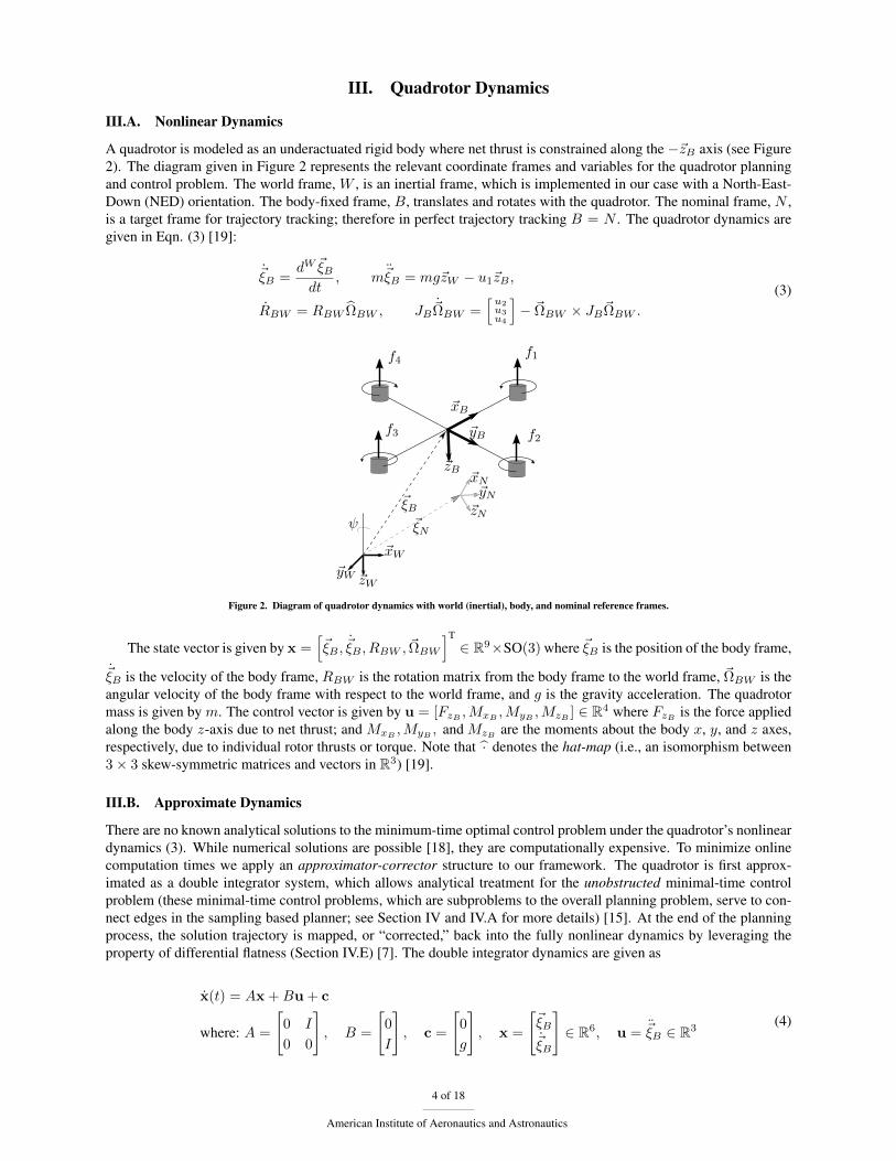
A quadrotor is modeled as an underactuated rigid body where net thrust is constrained along the −~zB axis (see Figure2). The diagram given in Figure 2 represents the relevant coordinate frames and variables for the quadrotor planningand control problem. The world frame, W , is an inertial frame, which is implemented in our case with a North-East-Down (NED) orientation. The body-fixed frame, B, translates and rotates with the quadrotor. The nominal frame, N ,is a target frame for trajectory tracking; therefore in perfect trajectory tracking B = N . The quadrotor dynamics aregiven in Eqn. (3) [19]:

~ξB =dW ~ξBdt

, m~ξB = mg~zW − u1~zB ,

RBW = RBW ΩBW , JB ~ΩBW =[u2u3u4

]− ~ΩBW × JB~ΩBW .

(3)

f1

f2f3

f4

~ξB

~zB

~xB

~yB

~xW

~yW ~zW

~ξNψ~zN

~xN~yN

Figure 2. Diagram of quadrotor dynamics with world (inertial), body, and nominal reference frames.

The state vector is given by x =[~ξB , ~ξB , RBW , ~ΩBW

]T∈ R9×SO(3) where ~ξB is the position of the body frame,

~ξB is the velocity of the body frame, RBW is the rotation matrix from the body frame to the world frame, ~ΩBW is theangular velocity of the body frame with respect to the world frame, and g is the gravity acceleration. The quadrotormass is given by m. The control vector is given by u = [FzB ,MxB

,MyB ,MzB ] ∈ R4 where FzB is the force appliedalong the body z-axis due to net thrust; and MxB

,MyB , and MzB are the moments about the body x, y, and z axes,respectively, due to individual rotor thrusts or torque. Note that · denotes the hat-map (i.e., an isomorphism between3× 3 skew-symmetric matrices and vectors in R3) [19].

III.B. Approximate Dynamics

There are no known analytical solutions to the minimum-time optimal control problem under the quadrotor’s nonlineardynamics (3). While numerical solutions are possible [18], they are computationally expensive. To minimize onlinecomputation times we apply an approximator-corrector structure to our framework. The quadrotor is first approx-imated as a double integrator system, which allows analytical treatment for the unobstructed minimal-time controlproblem (these minimal-time control problems, which are subproblems to the overall planning problem, serve to con-nect edges in the sampling based planner; see Section IV and IV.A for more details) [15]. At the end of the planningprocess, the solution trajectory is mapped, or “corrected,” back into the fully nonlinear dynamics by leveraging theproperty of differential flatness (Section IV.E) [7]. The double integrator dynamics are given as

x(t) = Ax +Bu + c

where: A =

[0 I

0 0

], B =

[0

I

], c =

[0

g

], x =

[~ξB~ξB

]∈ R6, u = ~ξB ∈ R3

(4)

4 of 18

American Institute of Aeronautics and Astronautics

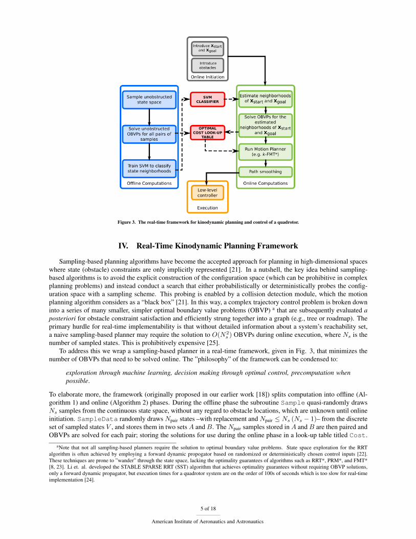
Figure 3. The real-time framework for kinodynamic planning and control of a quadrotor.

IV. Real-Time Kinodynamic Planning Framework

Sampling-based planning algorithms have become the accepted approach for planning in high-dimensional spaceswhere state (obstacle) constraints are only implicitly represented [21]. In a nutshell, the key idea behind sampling-based algorithms is to avoid the explicit construction of the configuration space (which can be prohibitive in complexplanning problems) and instead conduct a search that either probabilistically or deterministically probes the config-uration space with a sampling scheme. This probing is enabled by a collision detection module, which the motionplanning algorithm considers as a “black box” [21]. In this way, a complex trajectory control problem is broken downinto a series of many smaller, simpler optimal boundary value problems (OBVP) a that are subsequently evaluated aposteriori for obstacle constraint satisfaction and efficiently strung together into a graph (e.g., tree or roadmap). Theprimary hurdle for real-time implementability is that without detailed information about a system’s reachability set,a naive sampling-based planner may require the solution to O(N2

s ) OBVPs during online execution, where Ns is thenumber of sampled states. This is prohibitively expensive [25].

To address this we wrap a sampling-based planner in a real-time framework, given in Fig. 3, that minimizes thenumber of OBVPs that need to be solved online. The ”philosophy” of the framework can be condensed to:

exploration through machine learning, decision making through optimal control, precomputation whenpossible.

To elaborate more, the framework (originally proposed in our earlier work [18]) splits computation into offline (Al-gorithm 1) and online (Algorithm 2) phases. During the offline phase the subroutine Sample quasi-randomly drawsNs samples from the continuous state space, without any regard to obstacle locations, which are unknown until onlineinitiation. SampleData randomly draws Npair states –with replacement and Npair ≤ Ns (Ns − 1)– from the discreteset of sampled states V , and stores them in two sets A and B. The Npair samples stored in A and B are then paired andOBVPs are solved for each pair; storing the solutions for use during the online phase in a look-up table titled Cost.

aNote that not all sampling-based planners require the solution to optimal boundary value problems. State space exploration for the RRTalgorithm is often achieved by employing a forward dynamic propogator based on randomized or deterministically chosen control inputs [22].These techniques are prone to ”wander” through the state space, lacking the optimality guarantees of algorithms such as RRT*, PRM*, and FMT*[8, 23]. Li et. al. developed the STABLE SPARSE RRT (SST) algorithm that achieves optimality guarantees without requiring OBVP solutions,only a forward dynamic propagator, but execution times for a quadrotor system are on the order of 100s of seconds which is too slow for real-timeimplementation [24].

5 of 18

American Institute of Aeronautics and Astronautics

The OBVP solution subroutine, SolveOBVP, which is often referred to as a ”steering function” in the motion plan-ning literature, is given in Section IV.A. The look-up table Cost can equivalently be thought of as an precomputed,unobstructed roadmap (i.e. it is wholly ignorant of obstacle information which is not available until online initiation)through the state space. During the offline phase, a support vector machine (SVM) classifier, referred to as NearSVM,is trained using the look-up table Cost. The SVM provides query-based estimates of cost-limited reachable sets(i.e., neighborhoods) and is discussed in further details in Section IV.B. The cost threshold of the reachable set, oftenreferred to a ”neighborhood radius” in the motion planning literature, is the user defined value Jth.

Algorithm 1 Offline Phase for the Kinodynamic Motion Planning Framework1 V ← Sample(X , Ns)2 A← SampleData(V,Npair, replace)3 B ← SampleData(V,Npair, replace)4 Cost← SolveOBVP(A,B)5 NearSVM← TrainClassifier([A,B],Cost(A,B), Jth)

At the initiation of the online phase, obstacle data is presented along with the start state, xinit, and goal region,Xgoal

b. A set of Ngoal states are sampled from the goal region and stored in the discrete set Xgoal. The SVM classifieris used to rapidly approximate the outgoing neighborhood of xinit and the incoming neighborhood of Xgoal amongthe pre-sampled states; storing the sets in N out

init and storing in N ingoal, respectively (see Section IV.B for discussion on

outgoing and incoming neighborhoods). OBVPs are then solved from xinit and Xgoal to their nearest neighbors andthe solutions are stored in the look-up table. Note that this reduces the number of online OBVPs solved to O(1)!

The sampling-based planner, kino-FMT , is then called to return the optimal trajectory through the set of sampledstates, V , using the look-up table, or ”roadmap”, Cost. Though many candidate sampling-based planners could beused to compute a trajectory across this roadmap, we rely on the asymptotically-optimal (AO) FMT∗ algorithm forits efficiency (see [23] for a detailed discussion of the advantages of FMT∗ over state-of-the-art counterparts) andkinodynamic extension [26]. The Kinodynamic Fast Marching Trees algorithm (kino-FMT ) (adapted from [26])leverages the roadmap to efficiently determine the optimal sequence of sampled states to connect xinit and Xgoal,performing collision checking in real-time (see Section IV.C).

Algorithm 2 Online Phase for the Kinodynamic Motion Planning Framework1 Xgoal ← Sample(Xgoal, Ngoal)2 N out

init ← NearSVM(xinit, V \xinit, Jth)3 N in

goal ← NearSVM(V \Xgoal, Xgoal, Jth)4 for x ∈ V do5 if x ∈ N out

init then6 Cost← SolveOBVP(xinit, x)7 if x ∈ N in

goal then8 Cost← SolveOBVP(x,Xgoal)9 Path← kino-FMT (V,Cost, xinit, Xgoal)

10 return SmoothPath(Path)

Finally the sequence of states generated by kino-FMT is used as a set of waypoints for a path smoothing algorithmthat generates a minimum-snap, dynamically feasible trajectory for the quadrotor (see Section IV.D). Mapping thedifferentially flat output variables from the smooth trajectory back to the full state and control space (Section IV.E),we can provide feedforward terms to the flight controller (Section IV.F).

We now present the mathematical details for each of the framework components (to make the paper self-contained,we also state a number of results already available in the literature).

IV.A. Analytical Solution to OBVP

As explained in Section II, we minimize computations by approximating our system as the double integrator givenin Eqn (4). This approximation enables analytical solutions to the optimal boundary value problem between twosampled states, which is executed in the SolveOBVP algorithm. The approximation is corrected for in Section IV.E.The results in this section come from the works [15, 27].

bIf this information was available a priori, than all computations could be performed offline and the real-time implementation would becomeirrelevant.

6 of 18

American Institute of Aeronautics and Astronautics

To address control constraints on thrust, a control penalty term is added to the minimum-time cost function, thatis:

J [u, τ ] =

∫ τ

0

1 + u[t]TRuu[t] dt, (5)

where Ru ∈ Rm×m is symmetric positive definite. For a fixed final time, τ , the optimal cost J ∗ for the control-penalized double integrator model is given in closed form by Eqn. (6) where Ru = wRI and wR is the control penaltyweight [15, 27]:

J ∗[τ ] = τ + ‖x− x[τ ]‖Td[τ ]. (6)

The corresponding control and state trajectories as functions of time t, for a fixed final time τ , are given in Eqn.(7), respectively [15, 27]:

u[t] = R−1u BTexp

[AT(τ − t)

]d[τ ],

x[t] = x[t] +G[t]exp[AT(τ − t)

]d[τ ],

(7)

where

d[τ ] = G[τ ]−1 (x− x[τ ]) ,

G[t] =1

wR

t3/3 0 0 t2/2 0 0

0 t3/3 0 0 t2/2 0

0 0 t3/3 0 0 t2/2

t2/2 0 0 t 0 0

0 t2/2 0 0 t 0

0 0 t2/2 0 0 t

,x[t] = exp [At]x0 +

[0, 0, gt2/2, 0, 0, gt

]T,

(8)

Note that Eqns. (6) and (7) require a fixed final time τ The optimal final time τ∗ is found as argminJ [τ ],whichcan be solved for via a bisection search of Eqn. (6).

IV.B. Machine Learning of Neighborhoods

When the boundary states, xinit andXgoal, are introduced at online initiation they must be connected to the pre-sampledstates before the motion planner can execute. Naively connecting the terminal states to all pre-sampled states wouldrequire O(Ns) calls to SolveOBVP, which is prohibitively many to execute in real-time. Instead we seek to onlyconnect the boundary states with their nearest neighbors, as defined by the cost-limited reachable set (see Figure 4).By limiting edge connections from the boundary states to a fixed number of states in their respective neighborhoodswe have effectively reduced the number of online OBVPs to O(1). This reduction in online OBVPs lies at the core ofachieving real-time execution of a kinodynamic planner.

Figure 4. Conceptual representation of a cost-limited reachable set for a notional 2D dynamical system. Formally, a (forward) cost-limited reachable set is theset of states that can be reached from a given state with a cost bounded above by a given threshold (denoted as Jth).

7 of 18

American Institute of Aeronautics and Astronautics

A conceptual diagram of a cost-limited reachable set, i.e. neighborhood, of a given state is represented in Fig. 4.The mathematical definition of the “outgoing neighborhood” or forward cost-limited reachable set of a state xa is:

Rout (xa,U , Jth) := xb ∈ X | ∃u ∈ U and ∃t′ ∈ [t0, tf ] s.t. x (t′) = xb and J ∗ ≤ Jth, (9)

where Jth is a user-defined cost threshold. In plain English, the forward reachable set is the union of all states xb ∈ Xsuch that the optimal cost, J ∗, to steer the system from xa to xb is less than the cost threshold Jth. Also of importanceis the concept of an “incoming neighborhood” or backward reachable set. The backward reachable set of state xb isthe union of all states, xa, such that xb is in the forward reachable set of xa.

In general the determination of reachability sets is a computationally-expensive problem [28], therefore the real-time planning framework applies an approximation to the reachable sets based on machine learning. During the offlinephase a support vector machine (SVM) is trained with data stored in Cost and provides a query-based classificationof nearest neighbors. This approach leverage the authors’ prior work [29], which demonstrated the accuracy andefficiency of this procedure for a number of nonlinear dynamical systems.

To elaborate, we seek a function that makes a simple, binary discrimination:

is the optimal cost to traverse from an arbitrary state xa to an arbitrary state xb less than a giventhreshold Jth, or not?

To develop such a function, we leverage the data in Cost to provide training examples. A training example consistsof a initial state xa, final state xb, and optimal cost of traversal between the two. For each training example i =1, . . . , Ntrain where Ntrain ≤ Npair, the initial and final states are concatenated into an attribute vector p(i). If theoptimal cost of the training example is less than the user-defined threshold, Jth, then it is given a label y(i) = +1;otherwise it is given label y(i) = −1. The training of the SVM is accomplished with the optimization given in Eqn.(10) [30]:

maximizeα

Ntrain∑i=1

αi −1

2

Ntrain∑i,j=1

y(i)y(j)αiαjK(p(i),p(j)

)subject to 0 ≤ αi ≤ C, i = 1, . . . , Ntrain

m∑i=1

αiy(i) = 0

(10)

where the αi’s are Lagrange multipliers, C is a user-defined parameter that relaxes the requirement that the trainingexamples be completely separable, and K(·) is the kernel function. The vectors corresponding to non-zero Lagrangemultipliers αi’s are the support vectors. For this work the kernel function, K, has the form

K(p1,p2) =(φ (p1)

Tφ (p2) + c

)p,

where φ is a nonlinear mapping of the attribute vector to a feature vector, c is a weighting parameter between first andsecond order terms, and p is kernel order chosen by the user. Once the support vectors are obtained, predictions onreachability for a new OBVP, paramaterized by p, can be made with the predictor

NearSVM

(Ntrain∑i=1

αiy(i)K

(p(i), p

)+ b

). (11)

where b is a bias term that is determined as a function of the Lagrange multipliers [30].Note that NearSVM is trained on data in Cost which is generated with no knowledge of obstacle placement.

Therefore, NearSVM has no function in predicting obstacle collisions. Collision checking is solely within the realmof the sampling-based planner discussed in Section IV.C. Results on training and testing of the SVM classifier for aquadrotor system are presented in Section V.

IV.C. Sampling-Based Planner

The sampling-based motion planner at the core of our real-time framework is a kinodynamic variant of the FastMarching Tree (FMT∗ ) algorithm [23], and is presented in pseudo-code in Algorithm 3. The algorithm works by

8 of 18

American Institute of Aeronautics and Astronautics

expanding a tree, stored in a set of edge connections E, along the minimum cost-to-come front through the pre-sampled set of states V . The frontier of the tree is stored in set H and unconnected samples are stored in set W .

For each iteration of the algorithm, the minimum cost-to-come sample z is used as a pivot for exploration. Theforward-reachable set of z among the sampled states V is stored in the discrete set Nout

z . The intersection of Noutz

and set W is determined and the result is stored in set Xnear. Each sample, x ∈ Xnear, represents a candidate forexpansion of the tree. For each candidate x the backward reachable set among sampled states is determined and savedas set N in

x . The set Ynear is determined as the intersection of H and backward reachable set of x, N inx . The sample

ymin ∈ Ynear represents the optimal connection point (assuming no obstacles) between x and the existing tree. If theconnection from ymin and x is free of collisions with obstacles, then the (ymin, x) edge is added to the tree, x is addedto the frontier set H and removed from W . Once all nodes in Xnear are analyzed, the pivot node z is removed fromthe frontier set and the process is repeated. The algorithm succeeds in finding a path from xinit to Xgoal as soon as thecurrent pivot, z, is an element of Xgoal. If H ever becomes empty, then kino-FMT reports failure. The (asymptotic)optimality properties of FMT∗ (and its kinodynamic variants) are discussed in [23, 31, 26].

Algorithm 3 Kinodynamic Fast Marching Tree Algorithm (kino-FMT )1 V ← V ∪ xinit ∪ Xgoal2 E ← ∅3 W ← V \xinit; H ← xinit4 z ← xinit5 while z /∈ Xgoal do6 Nout

z ← Near(z, V \z, Jth)7 Xnear = Intersect(Nout

z ,W )8 for x ∈ Xnear do9 N in

x ← Near(V \x, x, Jth)10 Ynear ← Intersect(N in

x , H)11 ymin ← arg miny∈YnearCost(y, T = (V,E))+Cost(yx)12 if CollisionFree(ymin, x) then13 E ← E ∪ (ymin, x)14 H ← H ∪ x15 W ←W\x16 H ← H\z17 if H = ∅ then18 return Failure19 z ← arg miny∈HCost(y, T = (V,E))20 return Path(z, T = (V,E))

IV.D. Minimum-Snap Trajectory Smoother

Trajectory smoothing is commonly implemented in motion planning to improve the quality of the trajectory returnedby the planner. Furthermore, in our case, we need to correct for the double integrator approximation previously made.To this end we improve the sampling-based planner’s solution computed via kino-FMT by connecting the solutionsamples with a high-order polynomial spline. Building on Mellinger’s work [7], Richter et. al. [5] formulate the splinedetermination as an unconstrained quadratic programming problem that minimizes the integral of the square of thesnap (i.e. the 4th derivative of position); see Eqn. (12). In the unconstrained formulation, derivatives at samples of themotion plan, i.e. waypoints, are left as free parameters for optimization. For completeness we present the essentialresults of Richter as they are used in our current approach [5, 6].

Our goal in this section is to determine the coefficients of M polynomials of order N . These polynomials forma spline that is continuous up to the 4th derivative and passes through the sampled states, or “nodes”, of the solutiontrajectory determined in Section IV.C. While an infinite number of splines may exist that satisfy these conditions, weseek the spline that minimizes the integral of the square of the snap. Let us begin by considering a single polynomialP (t) =

∑Nn=0 pnt

n. The minimum-snap cost function for a single polynomial is defined as

Jsnap =

∫ T

0

P (4)(t)2 dt = pTQ(T )p, (12)

9 of 18

American Institute of Aeronautics and Astronautics

where Q(T ) is the Hessian matrix of Jsnap with respect to the polynomial coefficients, p is a vector of the N + 1polynomial coefficients, and T is the polynomial segment time which is determined by the kinodynamic planner.Without derivation, the Hessian matrix is given asc

Qi,j(T ) = 2

(3∏k=0

(i− k)(j − k)

)T i+j−7

i+ j − 7for: i ≥ 4 ∧ j ≥ 4,

Qi,j(T ) = 0 otherwise.

(13)

As previously mentioned, the polynomial is constrained at its terminal points, t = 0 and t = T , to the waypoints ofthe motion plan determined in Section IV.C. The derivatives of the polynomial at its terminal points can be fixed or leftas free parameters for optimization. Even as free parameters, however, the derivatives must satisfy continuity betweenpolynomials in the spline. These constraints can be encoded as the linear function

Ap = d (14)

A =

[A0

AT

], d =

[d0

dT

](15)

where the terms are given as

A0i,j=

∏i−1k=0(i− k) if i = j

0 if i 6= j(16)

d0i= P (i)(0) (17)

ATi,j=

(∏i−1

k=0(i− k))T i−j if i ≥ j

0 if i < j(18)

dTi= P (i)(T ) (19)

Numerical stability can be achieved by reformulating the constrained problem represented in Eqns. (12) and (15) asan unconstrained optimization [5, 6]. This is achieved by optimizing over the polynomial derivatives at the terminalpoints instead of the polynomial coefficients. Under this reformulation, Eqns. (12) and (15) become

Jsnap = dTA−TQ(T )A−1d, (20)

and the polynomial coefficients are determined, a posteriori, via inversion of Eqn. (14).Now that we have formulated the optimization problem for a single polynomial, we must consider the optimization

over the spline ofM polynomials. To this end we formA1...M andQ1...M which are block diagonal matrices composedof the A and Q matrices for each segment. We could also simply concatenate the derivative vectors into a vectord1...M , however it is desirable to separate this vector into components that are fixed and those that are free parametersof optimization. Therefore the derivative vector for the spline optimization is formed as

dtotal =

[dfix

dfree

]. (21)

With this reordering of the derivative vector in Eqn. (21), an ordering matrix C is required that preserves the properrelationships with the block matrices A1...M and Q1...M . Furthermore, the ordering matrix C also encodes the en-forcement of continuity of derivatives at intermediate waypoints. Now the minimum-snap cost function for the entirespline is given as

Jsnap = dTtotalCA

−T1...MQ1...MA1...MC

Tdtotal. (22)

cNote that we diverge from Richter by only considering the minimization on the 4th derivative, where Richter leaves the formulation moregeneral as a weighted sum of squares of derivatives. Furthermore, due to the fact that Richter uses a geometric planner to determine waypoints, hisapproach requires a time allocation optimization to determine polynomial segment times, T [5, 6]. In contrast, our work determines the polynomialsegment times during the time-minimizing kinodynamic planning; see Section IV.C.

10 of 18

American Institute of Aeronautics and Astronautics

For simplicity, define the matrix H = CA−T1...MQ1...MA1...MC

T and partition it such that Eqn. (22) can be written

Jsnap =

[dfix

dfree

]T [H11 H12

H21 H22

][dfix

dfree

]. (23)

Differentiating and setting to zero solves for the free derivatives at the waypoints

d∗free = −H−122 H

T12dfix. (24)

Now that the derivatives at each waypoint are determined, the polynomial coefficients can be determined by invertingEqn. (14). This process is applied for the determination of four splines: x, y, and z positions and yaw. These splinescorrespond to the differential flat output variables discussed in Section IV.E.

It is important to note here that once smoothing is applied, the trajectory is no longer guaranteed to be collisionfree. Therefore it is necessary to perform an additional collision checking phase during the trajectory smoothingphase. If one of the polynomials in the spline is found to collide with an obstacle, then a new smoothed trajectorymust be determined. This is accomplished by sampling the midpoint of the underlying motion plan solution which isguaranteed to be collision free (else it would have not been selected as a valid motion plan). The trajectory smootherthan solves the minimum-snap optimization problem forM+1 trajectory segments. This is repeated until the smoothedtrajectory is collision free. See Richter et. al. for more details [5, 6].

IV.E. Differentially Flat Mapping

The trajectory smoother from Section IV.D produces polynomial splines for position and yaw that are continuous upto their fourth derivative. Mellinger et. al. showed that the state and control variables for the nonlinear quadrotordynamics can be expressed in terms of ~ξN and ψN and their derivatives up to fourth order; thus proving Eqn. (3)represents a differentially flat system with flat output variables ~ξN and ψN [7]. This mathematical property provesthat the smoothed trajectory from Section IV.D is guaranteed to be dynamically feasible for the quadrotor; thereforecorrecting the double-integrator approximation made to solve the planning problem. For completeness we state theresults of Mellinger et. al. for the mapping from the flat outputs to the nominal state and control variables. Note that,while the following equations are taken almost directly from [7], there are some subtle coordinate frame changes.

The nominal position and velocity state variables are identically ~ξN and ~ξN , respectively. The thrust controlvariable is given as

u1ff= −~zB · ~FN , where: ~FN = m~ξN −mg~zW (25)

The subscript ff indicate that this thrust value appears as a feedforward term in the flight controller (Section IV.F).The nominal orientation matrix is given by the nominal frame axes represented in world coordinates:

~RN =[W~xN ,

W~yN ,W~zN

], (26)

where

~zN = −~FN

‖~FN‖~yS = [−sinψN , cosψN , 0]

T

~xN =~yS × ~zN‖~yS × ~zN‖

~yN = ~zN × ~xN .

(27)

The nominal angular velocity vector is given by

~ΩNW = pN~xN + qN~yN + rN~zN (28)

where the individual components of nominal angular velocity are

11 of 18

American Institute of Aeronautics and Astronautics

pN = −~hΩ · ~yNqN = ~hΩ · ~xNrN = ψN~zW · ~zN

(29)

For compactness we have defined

~hΩ =m

u1ff

((~ξ

(3)N · ~zN

)~zN − ~ξ(3)

N

)(30)

The nominal angular acceleration, used in the calculation of the feedforward moment terms, is derived to be

~ΩNW = α1N~xN + α2N

~yN + α3N~zN (31)

where the individual components of nominal angular acceleration are

α1N= −~hα · ~yN

α2N= ~hα · ~xN

α3N=(ψN~zN − ψN~hΩ

)· ~zW

(32)

Again for compactness we give

~hα = − 1

u1ff

(m~ξ

(4)N + u1ff

~zN + 2u1ff~ΩNW × ~zN

+~ΩNW × ~ΩNW × ~zN) (33)

The derivative of the net thrust, which appear in Eqn (33), are derived to be

u1ff= −m~ξ(3)

N · ~zN

u1ff= −

(m~ξ

(4)N + ~ΩNW × ~ΩNW × ~zN

)· ~zN

(34)

Note that the equations presented in this section are taken almost directly from Mellinger et. al. [7] but are stated herefor completeness of our approach.

IV.F. Flight Controller

The flight controller is based on work by Lee et. al. and can be consider a form of feedforward/feedback control [19].Feedforward inputs, denoted with subscript ff , are generated from the differentially flat mapping in Section IV.Eand feedback terms, denoted with subscript fb, are generated via proportional-derivative (PD) tracking of position,velocity, orientation and angular velocity. Equation (35) gives the net thrust control input.

u1 = u1ff+ u1fb

= −~zB ·(m~ξN −mg~zW +Kξ~exi+Kv~ev

) (35)

Equation (36) presents the control inputs for the moments about the body axes.

[u2, u3, u4]T

= [u2, u3, u4]Tff + [u2, u3, u4]

Tfb

= JB

(RTBRN

~ΩBW − ~ΩBW ×(RTBRN ~ΩBW

))+ ~ΩBW × JB~ΩBW +KR~eR +KΩ~eΩ

(36)

The error terms for feedback control are given by Eqn. (37) [19]

12 of 18

American Institute of Aeronautics and Astronautics

~eξ = ~ξN − ~ξ

~ev = ~ξN − ~ξ

~eR =1

2

(RTBRD −RT

DRB)∨

~eΩ = RTBRD~ΩD − ~ΩB

(37)

where ∨ represents the vee-map; the inverse of the hat-map. The matrices Kξ,Kv,KR,KΩ ∈ R3×3 are user-definedgain matrices for PD trajectory tracking.

V. Experimental Results

V.A. Experimental Setup

The real-time framework is demonstrated on a Pixhawk autopilot flown on a DJI F-450 frame. Positioning informationis provided by a Vicon motion tracker with data streamed to the quadrotor via a Wifly RN-XV module. Currently themotion planning and path smoothing computations are run in MATLAB/C++ on a single-threaded Intel Core i7-4790KCPU. The final trajectory is transmitted to the Pixhawk for low-level flight control. This communication structure isrepresented in Fig. 5. Table 1 gives detailed information on the computational platform and programming languagefor each of the major components of the framework discussed in Section IV. Future work will convert all portions ofthe online phase (see Alg. 2) to C++ to be run on an embedded processor on the quadrotor.

Table 1. Computational platform and programming language for the major components of the real-time framework.

Process Reference Processor Languagelocalization NA workstation C++

precomputations IV workstation MATLABneighborhood estimation IV.B workstation MATLAB

OBVP solutions IV.A workstation MATLABsampling-based planning IV.C workstation C++

min-snap smoothing IV.D workstation MATLABflat-to-nonlinear mapping IV.E Pixhawk C/C++

flight control IV.F Pixhawk C/C++

The quadrotor is navigating an indoor environment with dimensions of approximately 3m×4m×3m. The obstacleset consists of two parrallel walls with 1.5m openings at opposite ends and a 1.5m separating corridor. This obstacleset is designed to be similar in form to that presented by Webb and van den Berg [15].

Figure 5. Communication/computation structure for flight tests.

13 of 18

American Institute of Aeronautics and Astronautics

V.B. Numerical Results and Flight Data

The real-time kinodynamic planner was successfully demonstrated in flight tests. The first image in Fig 6 givesan overhead view of the exploration tree generated by kino-FMT during execution with the final solution shown inblue. The second image in Fig 6 compares the minimum-time, sampling-based motion plan; minimum-snap smoothedtrajectory of the differentially flat output variables; and the flight trajectory that was physically flown by the quadrotor.Fig 7 shows a set of screen captures from a recording of the flight.

Figure 6. (left) Tree explored by the kino-FMT algorithm with optimal solution in blue. (right) Motion plan (blue), smoothed trajectory (multi-colored), andflight data (green) shown with the parallel wall obstacles.

The primary goal of this work was to prove that the entire planning framework can be executed in a real-timeenvironment. The computational timing data and path cost are given in Table 2 for a range of sampled states. Itis shown that the entire kinodynamic planning and control problem can be solved in under 1/3 of a second for 500sampled nodes. Even with 3000 sampled states, the computation time for the entire planner is under 2 seconds.

To compare this to existing results, Webb and van den Berg simulate an almost identical problem; however they donot perform any path smoothing or communication to a physical quadrotor [15]. With 1000 sampled states Webb andvan den Berg’s solution takes 51.603 seconds; i.e. 120x, or 2 orders of magnitude, slower than the technique presentedhere. Richter et. al. do not state the computation time for motion plan demonstrated in their work [5]. They do,however, give the computation time for a simplified, 2-dimensional problem that incorporates geometric path planningand minimum-snap path smoothing. Richter’s simplified, 2D planning problem takes 3 seconds of computation time;i.e. 9.6x, or 1 order of magnitude, slower than the fastest computation time presented here. Therefore the real-time kinodynamic framework demonstrates a significant reduction in computation time when compared to existingtechniques.

Frazzoli et. al. boasts the most impressive computation times with sub-second execution for the similar, but notidentical, helicopter system navigating spherical objects [11]. Computation times for a parallel wall obstacle set riseinto the 10s of seconds, however Frazzoli is considering the more challenging situation of dynamic obstacles. Directcomparison with Frazzoli’s work is more difficult because it only seeks feasible trajectories, not necessarily optimalones. The work employs only a small set of motion primitives - avoiding the solution to online OBVPs all together -to achieve path planning. Restricting trajectories to a small set of predefined maneuvers limits the technique’s abilityto handle novel, complex, or even pathological obstacle environments.

In Table 2 the computation time is broken down into percentages for the major components of the framework:neighborhood classification for the terminal states (see Sec. IV.B); neighborhood OBVP solutions for the terminalstates (see Sec. IV.A); sampling-based motion planning (see Sec. IV.C); path smoothing to generate a minimum-snap, dynamically feasible trajectory (see Sec. IV.D); and communication (see Sec. V.A). We see that the majority ofthe computation time is consumed by the solution of optimal boundary value problems between the terminal states,xinit and the samples in Xgoal, and their estimated neighborhoods. This result exemplifies the motivation to minimizethe number of online OBVPs to be solved. For the double integrator model of the quadrotor, the average OBVPsolution time is 0.0235 seconds per OBVP solution. In comparison, the average NearSVM classification time is

14 of 18

American Institute of Aeronautics and Astronautics

Table 2. Path cost and computation time breakdown for the Real-Time Kinodynamic Framework for differing numbers of sampled states

# ofSamples

PathCost [s]

ComputationTime [s]

NeighborClassifier [%]

NeighborOBVPs [%]

Kino-FMT*[%]

Smoothing[%]

Comms[%]

500 5.4958 0.3125 6.42 37.73 9.43 30.43 25.291000 5.4721 0.4293 5.31 41.01 13.60 32.70 4.242000 5.2382 0.9242 4.56 41.65 19.81 26.40 3.383000 5.2910 1.789 3.08 53.69 29.74 9.65 1.63

1.95×10−5 seconds per classification; roughly 1200 times, or three orders of magnitude, faster than OBVP solution.This rapid approximation of neighborhood sets as –opposed to explicit determination via OBVP solutions– is thecritically enabling component for real-time implementation.

Table 3. Feature vector for neighbor determination of the double integrator quadrotor model.

x1 x2 |∆x| (∆x)2 (∆x)3√

(∆x)2 + (∆y)2 + (∆z)2

y1 y2 |∆y| (∆y)2 (∆y)3√

(∆x)2 + (∆y)2 + (∆z)2

z1 z2 |∆z| (∆z)2 (∆z)3√

(∆x)2 + (∆y)2 + (∆z)2 + (∆x)2 + (∆y)2 + (∆z)2

x1 x2 |∆x| (∆x)2 (∆x)3

y1 y2 |∆y| (∆y)2 (∆x)3

z1 z2 |∆z| (∆z)2 (∆x)3

Due to the reliance on machine-learning of neighbor sets, it is important to determine the classification accuracy ofthe NearSVM algorithm. The feature vector is a 33-element vector, given in Table 3, composed of nonlinear mappingsof the boundary value state variables. A third order kernel function is chosen; therefore p = 3 in Eqn. (11). Fortraining and testing of the SVM classifier 50000 OBVPs are solved from randomly selected pairs of sampled statesduring the offline computation phase. A neighbor radius, or cost threshold, is chosen as the 10th quantile of all OBVPcosts; which for this test campaign evaluated to neighbor cost threshold of roughly 0.69 seconds. In other words, for agiven state, roughly 10% of all other states are within 0.69 seconds as measured by a minimum-time optimal controlproblem. To train the SVM classifier, Ntrain = 20000 of the 50000 OBVP solutions were used with the 0.69 secondcost threshold. On average less than one training error occurred per the 20000 training examples. The algorithmwas tested against 30000 additional OBVP examples to ensure that the SVM was not over-trained to the training setd. The average testing error was under 3%, well within the acceptable tolerance for the purpose of this work and amarked improvement over the author’s prior work on machine learning of cost-limited reachable sets [29]. Table 4gives the training and testing results. A ‘positive’ indicates that NearSVM classified the OBVP example as withinthe cost threshold, and a ‘negative’ indicates a classification of the OBVP outside of the cost threshold. The numberof true positives is roughly 10% of the number of true negatives; as expected with the 10th quantile cost threshold.The average number of false positives and false negatives are approximately equal indicating that the classifier is notbiased toward one classificatione.

Table 4. Training and testing accuracy of machine-learning-based neighborhood classification algorithm

# TrainingExamples

Avg. #TrainingErrors

# TestingExamples

Avg. #True

Positives

Avg. #True

Negatives

Avg. #False

Positives

Avg. #False

Negatives

TestingError [%]

20000 0.6 30000 2693 26600.6 371.8 334.6 2.35

dTypically the training set would be much larger than the testing set, but due to convergence issues while training, the training set was reducedand the remainder of OBVP examples was dedicated to the testing set.

eFor example, we could use a trivial classifier that only predicted negatives and it would return a testing error of 10% because only 10% of casesare positive. This would actually constitute an acceptable rate of classification error if it were not for the fact that all errors would be false negativesas the the classifier is trivial. Therefore a well trained classifier should not be biased toward one type of error.

15 of 18

American Institute of Aeronautics and Astronautics

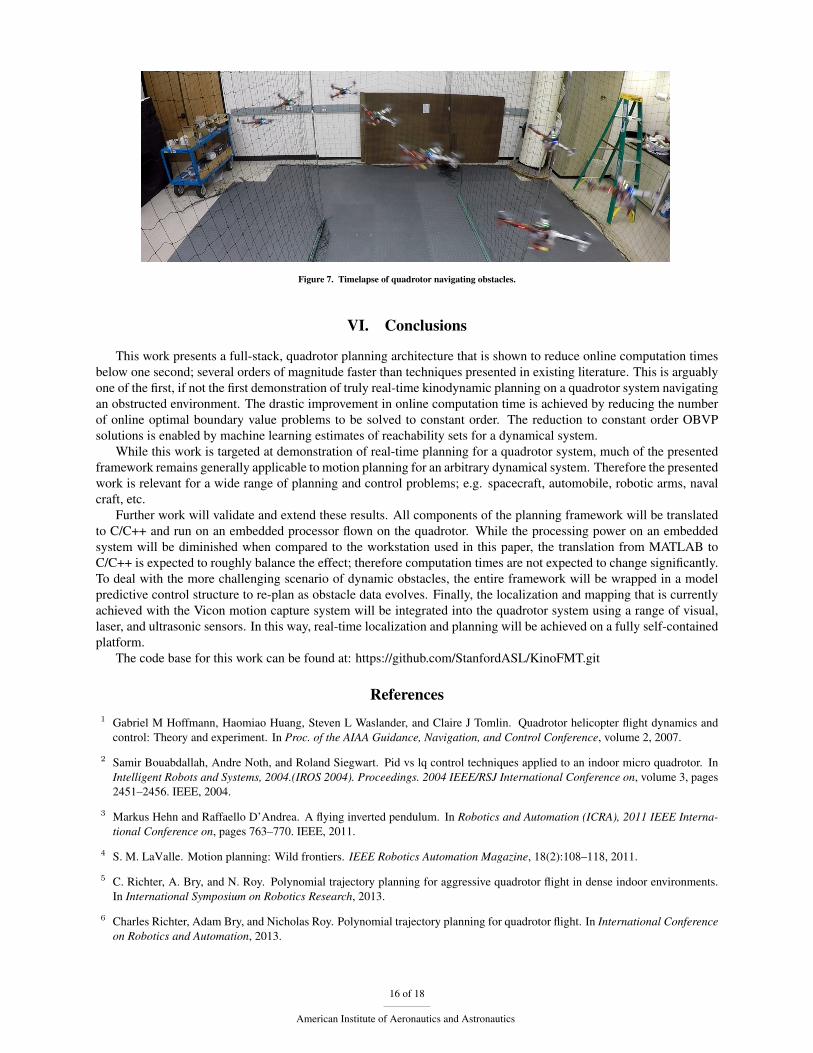
Figure 7. Timelapse of quadrotor navigating obstacles.

VI. Conclusions

This work presents a full-stack, quadrotor planning architecture that is shown to reduce online computation timesbelow one second; several orders of magnitude faster than techniques presented in existing literature. This is arguablyone of the first, if not the first demonstration of truly real-time kinodynamic planning on a quadrotor system navigatingan obstructed environment. The drastic improvement in online computation time is achieved by reducing the numberof online optimal boundary value problems to be solved to constant order. The reduction to constant order OBVPsolutions is enabled by machine learning estimates of reachability sets for a dynamical system.

While this work is targeted at demonstration of real-time planning for a quadrotor system, much of the presentedframework remains generally applicable to motion planning for an arbitrary dynamical system. Therefore the presentedwork is relevant for a wide range of planning and control problems; e.g. spacecraft, automobile, robotic arms, navalcraft, etc.

Further work will validate and extend these results. All components of the planning framework will be translatedto C/C++ and run on an embedded processor flown on the quadrotor. While the processing power on an embeddedsystem will be diminished when compared to the workstation used in this paper, the translation from MATLAB toC/C++ is expected to roughly balance the effect; therefore computation times are not expected to change significantly.To deal with the more challenging scenario of dynamic obstacles, the entire framework will be wrapped in a modelpredictive control structure to re-plan as obstacle data evolves. Finally, the localization and mapping that is currentlyachieved with the Vicon motion capture system will be integrated into the quadrotor system using a range of visual,laser, and ultrasonic sensors. In this way, real-time localization and planning will be achieved on a fully self-containedplatform.

The code base for this work can be found at: https://github.com/StanfordASL/KinoFMT.git

References1 Gabriel M Hoffmann, Haomiao Huang, Steven L Waslander, and Claire J Tomlin. Quadrotor helicopter flight dynamics and

control: Theory and experiment. In Proc. of the AIAA Guidance, Navigation, and Control Conference, volume 2, 2007.

2 Samir Bouabdallah, Andre Noth, and Roland Siegwart. Pid vs lq control techniques applied to an indoor micro quadrotor. InIntelligent Robots and Systems, 2004.(IROS 2004). Proceedings. 2004 IEEE/RSJ International Conference on, volume 3, pages2451–2456. IEEE, 2004.

3 Markus Hehn and Raffaello D’Andrea. A flying inverted pendulum. In Robotics and Automation (ICRA), 2011 IEEE Interna-tional Conference on, pages 763–770. IEEE, 2011.

4 S. M. LaValle. Motion planning: Wild frontiers. IEEE Robotics Automation Magazine, 18(2):108–118, 2011.

5 C. Richter, A. Bry, and N. Roy. Polynomial trajectory planning for aggressive quadrotor flight in dense indoor environments.In International Symposium on Robotics Research, 2013.

6 Charles Richter, Adam Bry, and Nicholas Roy. Polynomial trajectory planning for quadrotor flight. In International Conferenceon Robotics and Automation, 2013.

16 of 18

American Institute of Aeronautics and Astronautics

7 D. Mellinger and V. Kumar. Minimum snap trajectory generation and control for quadrotors. In Proc. IEEE Conf. on Roboticsand Automation, pages 2520–2525, 2011.

8 S. Karaman and E. Frazzoli. Sampling-based algorithms for optimal motion planning. International Journal of RoboticsResearch, 30(7):846–894, 2011.

9 Koushil Sreenath, Taeyoung Lee, and Vipin Kumar. Geometric control and differential flatness of a quadrotor UAV with acable-suspended load. In Decision and Control (CDC), 2013 IEEE 52nd Annual Conference on, pages 2269–2274. IEEE, 2013.

10 Daniel Mellinger, Nathan Michael, and Vijay Kumar. Trajectory generation and control for precise aggressive maneuvers withquadrotors. The International Journal of Robotics Research, page 0278364911434236, 2012.

11 E. Frazzoli, M. A. Dahleh, and E. Feron. Real-time motion planning for agile autonomous vehicles. AIAA Journal of Guidance,Control, and Dynamics, 25(1):116–129, 2002.

12 Ian D Cowling, Oleg A Yakimenko, James F Whidborne, and Alastair K Cooke. Direct method based control system for anautonomous quadrotor. Journal of Intelligent & Robotic Systems, 60(2):285–316, 2010.

13 Ian D Cowling, Oleg A Yakimenko, James F Whidborne, and Alastair K Cooke. A prototype of an autonomous controller fora quadrotor UAV. In Control Conference (ECC), 2007 European, pages 4001–4008. IEEE, 2007.

14 Y Bouktir, M Haddad, and T Chettibi. Trajectory planning for a quadrotor helicopter. In Control and Automation, 2008 16thMediterranean Conference on, pages 1258–1263. IEEE, 2008.

15 D. J. Webb and J. van den Berg. Kinodynamic RRT*: Optimal Motion Planning for Systems with Linear Differential Con-straints. In Proc. IEEE Conf. on Robotics and Automation, pages 5054–5061, 2013.

16 Benoit Landry. Planning and Control for Quadrotor Flight Through Cluttered Environments. Master’s thesis, MassachusettsInstitute of Technology, 2015.

17 Slawomir Grzonka, Giorgio Grisetti, and Wolfram Burgard. A fully autonomous indoor quadrotor. Robotics, IEEE Transactionson, 28(1):90–100, 2012.

18 Ross Allen and Marco Pavone. Toward a Real-Time Framework for Solving the Kinodynamic Motion Planning Problem. InProc. IEEE Conf. on Robotics and Automation, Seattle, WA, May 2015. In Press.

19 Taeyoung Lee, Melvin Leok, and N Harris McClamroch. Nonlinear robust tracking control of a quadrotor UAV on SE (3).Asian Journal of Control, 15(2):391–408, 2013.

20 John Schulman, Jonathan Ho, Alex Lee, Ibrahim Awwal, Henry Bradlow, and Pieter Abbeel. Finding Locally Optimal,Collision-Free Trajectories with Sequential Convex Optimization. In Robotics: Science and Systems, volume 9, pages 1–10.Citeseer, 2013.

21 S. Lavalle. Planning Algorithms. Cambridge University Press, 2006.

22 S. M. LaValle and J. J. Kuffner. Randomized Kinodynamic Planning. International Journal of Robotics Research, 20(5):378–400, 2001.

23 Lucas Janson, Edward Schmerling, Ashley Clark, and Marco Pavone. Fast Marching Tree: A Fast Marching Sampling-BasedMethod for Optimal Motion Planning in Many Dimensions. International Journal of Robotics Research, 34(7):883–921, 2015.

24 Yanbo Li, Zakary Littlefield, and Kostas E Bekris. Asymptotically optimal sampling-based kinodynamic planning. arXivpreprint arXiv:1407.2896, 2014.

25 I Michael Ross and Fariba Fahroo. Issues in the real-time computation of optimal control. Mathematical and computer mod-elling, 43(9):1172–1188, 2006.

26 E. Schmerling, L. Janson, and M. Pavone. Optimal Sampling-Based Motion Planning under Differential Constraints: the DriftCase with Linear Affine Dynamics. In Proc. IEEE Conf. on Decision and Control, 2015. In Press.

27 Edward Schmerling, Lucas Janson, and Marco Pavone. Optimal Sampling-Based Motion Planning under Differential Con-straints: the Drift Case with Linear Affine Dynamics (Extended Version). Available at http://arxiv.org/abs/1405.7421/, May 2015.

28 D. M. Stipanovic, I. Hwang, and C. J. Tomlin. Computation of an Over-Approximation of the Backward Reachable Set UsingSubsystem Level Set Functions. Dynamics of Continuous Discrete and Impulsive Systems, 11:397–412, 2004.

17 of 18

American Institute of Aeronautics and Astronautics

29 Ross Allen, Ashley Clark, Joseph Starek, and Marco Pavone. A Machine Learning Approach for Real-Time ReachabilityAnalysis. In IEEE/RSJ Int. Conf. on Intelligent Robots & Systems, pages 2202–2208, Chicago, IL, September 2014.

30 Christopher M Bishop. Pattern recognition and machine learning. Springer, 2006.

31 E. Schmerling, L. Janson, and M. Pavone. Optimal Sampling-Based Motion Planning under Differential Constraints: theDriftless Case. In Proc. IEEE Conf. on Robotics and Automation, pages 2368–2375, 2015.

18 of 18

American Institute of Aeronautics and Astronautics