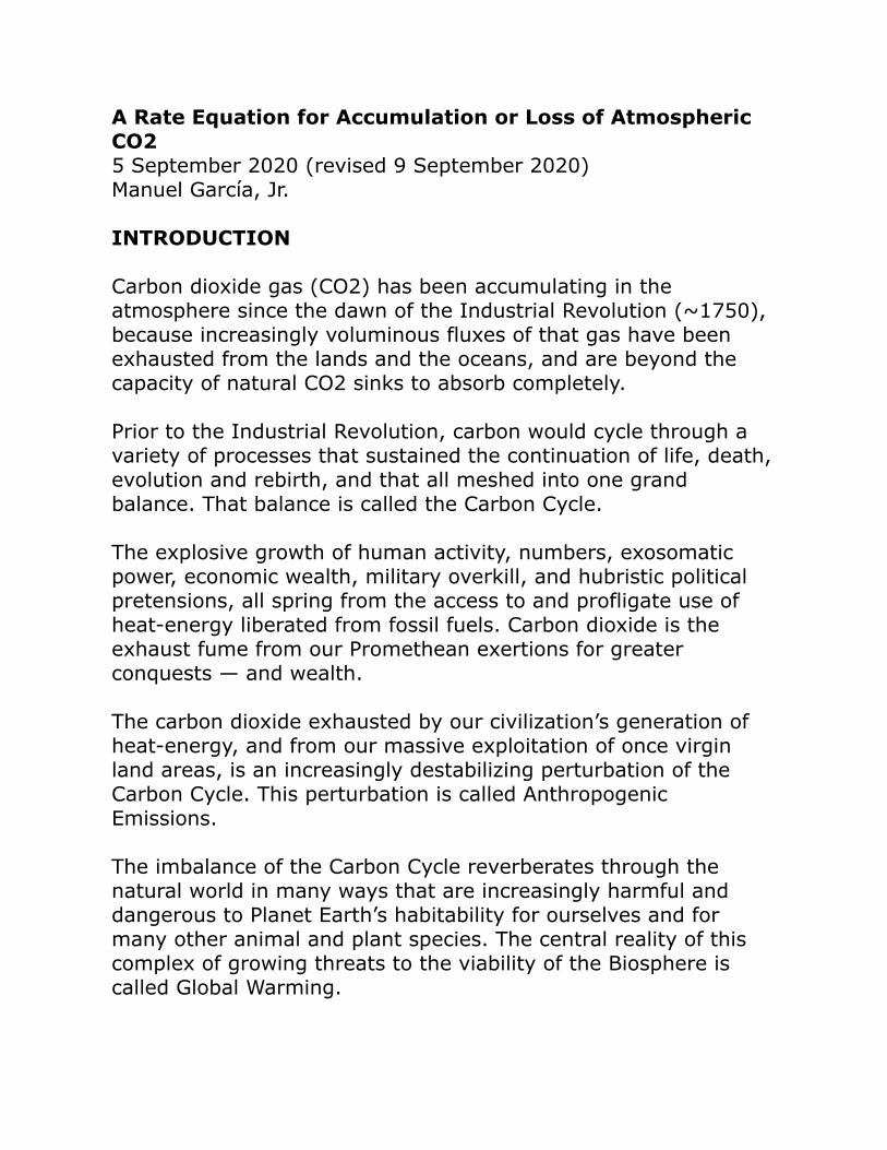
A Rate Equation for Accumulation or Loss of Atmospheric CO25 September 2020 (revised 9 September 2020)Manuel García, Jr.

INTRODUCTION

Carbon dioxide gas (CO2) has been accumulating in the atmosphere since the dawn of the Industrial Revolution (~1750), because increasingly voluminous fluxes of that gas have been exhausted from the lands and the oceans, and are beyond the capacity of natural CO2 sinks to absorb completely.

Prior to the Industrial Revolution, carbon would cycle through a variety of processes that sustained the continuation of life, death, evolution and rebirth, and that all meshed into one grand balance. That balance is called the Carbon Cycle.

The explosive growth of human activity, numbers, exosomatic power, economic wealth, military overkill, and hubristic political pretensions, all spring from the access to and profligate use of heat-energy liberated from fossil fuels. Carbon dioxide is the exhaust fume from our Promethean exertions for greater conquests — and wealth.

The carbon dioxide exhausted by our civilization’s generation of heat-energy, and from our massive exploitation of once virgin land areas, is an increasingly destabilizing perturbation of the Carbon Cycle. This perturbation is called Anthropogenic Emissions.

The imbalance of the Carbon Cycle reverberates through the natural world in many ways that are increasingly harmful and dangerous to Planet Earth’s habitability for ourselves and for many other animal and plant species. The central reality of this complex of growing threats to the viability of the Biosphere is called Global Warming.

Carbon dioxide gas traps heat radiated towards space, as infrared radiation from the surface of Planet Earth, reducing our planet’s ability to regulate its temperature by cooling to compensate for the influx of solar light that is absorbed by the lands and the oceans, and stored by them as heat.

Because of the existential implications of runaway global warming — as well as the intrinsic fascination to curious minds of such a richly complex and grand human-entwined natural phenomenon — scientists have been studying global warming, and its impact on the biosphere, which is called Climate Change.

While scientists of all kinds are excited to share their findings on climate change and impress their colleagues with their new insights, members of the public are singularly interested to know how climate change will affect their personal futures. Can science offer them clear and reliable answers to their questions — and fears — and provide practical remedies and technological inoculations to ward off the threats by climate change to our existing ways of life?

Science does what it can to offer practical insights and helpful recommendations, and humanity does what it usually does when faced with a collective existential crisis: it hides from the inconvenience of drastically changing its personal attitudes and societal structures, which is in fact the only way it would be able to navigate the majority of Earth’s people through the transition to a new social paradigm; a new, sustainable and harmonious relationship between human life and Planet Earth.

While I am grateful to all the professional climate scientists — and their related life scientists who study many aspects of this complex of geophysical processes and biological organisms and systems — for making known so much of the workings of the globally warming biosphere, I am nevertheless curious to gain a quantitative understanding of it all for myself. To that end, I have devised my own phenomenological thermodynamic “toy models” of global warming. The sequence of my reports charting the

evolution of my quantitative understanding of global warming, are listed at:

<><><><><><><>

One Year of Global Warming Reports by MG,Jr15 July 2020https://manuelgarciajr.com/2020/07/15/one-year-of-global-warming-reports-by-mgjr/

Updated to 2 September 2020

<><><><><><><>

The present report will describe a rate equation for the accumulation or loss of atmospheric CO2 over the course of future time. This equation is derived from considerations of recent data on the Carbon Cycle, along with some mathematical assumptions about the relationships used to quantify “carbon dioxide sweepers,” the processes that scavenge atmospheric CO2.

The results of this work are projections of possible future histories of the concentration of atmospheric carbon dioxide, as well as a projection of the most likely trend of rising average global temperature. As is true of all future-casts, we will just have to wait till then to see if they were accurate, assuming we don’t do anything beforehand — collectively — to avoid the worst possibilities. Such is the dance with the chaos and nonlinearity of the approaching future.

TABLE OF CONTENTS

- Introduction- Units and Data- General Form of the Rate Equation- Sinks- Long-term CO2 Sweepers and the PETM

- Rate Equation for the Accumulation or Loss of Atmospheric CO2- Case #1, “business as usual”- Case #2, “flat” at 407.4ppm- Case #3, “maximum loss”- Temperature Rise for “Business as Usual”- Proportionalities- Graphs

UNITS AND DATA

All quantities of material bulk will be shown in units of Giga-tonnes of carbon dioxide (GtCO2). A tonne is a metric unit of mass equivalent to 1000 kilograms.

The concentration of carbon dioxide gas in the atmosphere will be described either in GtCO2, or in parts-per-million-by-volume (ppm).

The rate at which CO2 is emitted into or scavenged from the atmosphere will be expressed as either GtCO2-per-year (GtCO2/y) or ppm-per-year (ppm/y).

Temperature change relative to the pre-industrial world will be shown as degrees Centigrade (°C) above the average global temperature in, say, 1850 to 1910.

In the descriptions to follow, units will explicitly accompany numerical quantities so as to avoid any confusion.

Following are 5 pages from the Global Carbon Project (GCP, https://www.globalcarbonproject.org/carbonbudget/) showing most of the data used in this report; along with a graphic constructed (by others) from the data in the IPCC reports of 2007, showing a summary of the average operation of the Carbon Cycle between 1958 and 2004.

GtC (Giga-tonnes-carbon) to GtCO2 units conversion

Global Fossil CO2 Emissions (1990-2019)

Atmospheric CO2 Concentration (1960-2018)

Anthropogenic Perturbation of the Carbon Cycle (2009-2018)

Global Carbon Budget 2019 (Infographic)

and

Anthropogenic Perturbation of the Carbon Cycle (IPCC 2007).

<><><><><><><>

All the data is shown in billion tonnes CO2 (GtCO2)

1 Gigatonne (Gt) = 1 billion tonnes = 1×1015g = 1 Petagram (Pg)

1 kg carbon (C) = 3.664 kg carbon dioxide (CO2)

1 GtC = 3.664 billion tonnes CO2 = 3.664 GtCO2

(Figures in units of GtC and GtCO2 are available from http://globalcarbonbudget.org/carbonbudget)

Most figures in this presentation are available for download as PNG filesfrom tinyurl.com/GCB19figs along with the data required to produce them.

DisclaimerThe Global Carbon Budget and the information presented here are intended for those interested in

learning about the carbon cycle, and how human activities are changing it. The information contained herein is provided as a public service, with the understanding that the Global Carbon Project team make

no warranties, either expressed or implied, concerning the accuracy, completeness, reliability, or suitability of the information.

The 2019 projection is based on preliminary data and modelling.Source: CDIAC; Friedlingstein et al 2019; Global Carbon Budget 2019

Global Fossil CO2 Emissions

Uncertainty is ±5% for one standard deviation

(IPCC “likely” range)

Global fossil CO2 emissions: 36.6 ± 2 GtCO2 in 2018, 61% over 1990 Projection for 2019: 36.8 ± 2 GtCO2, 0.6% higher than 2018 (range -0.2% to 1.5%)

Fossil CO2 emissions will likely be more than 4% higher in 2019 than the year of the Paris Agreement in 2015

Atmospheric concentration

The global CO2 concentration increased from ~277ppm in 1750 to 407ppm in 2018 (up 46%)2016 was the first full year with concentration above 400ppm

Globally averaged surface atmospheric CO2 concentration. Data from: NOAA-ESRL after 1980; the Scripps Institution of Oceanography before 1980 (harmonised to recent data by adding 0.542ppm)

Source: NOAA-ESRL; Scripps Institution of Oceanography; Friedlingstein et al 2019; Global Carbon Budget 2019

Anthropogenic perturbation of the global carbon cycle

Perturbation of the global carbon cycle caused by anthropogenic activities,averaged globally for the decade 2009–2018 (GtCO2/yr)

The budget imbalance is the difference between the estimated emissions and sinks. Source: CDIAC; NOAA-ESRL; Friedlingstein et al 2019; Ciais et al. 2013; Global Carbon Budget 2019

Copyright:

Global Carbon Budget 2019Fossil CO2 emissions grow more slowly... but do not yet decline

Natural gas and oil now drive global emissions growth

The rise in atmospheric CO2 causes climate change

CoalOilGas Land

Emissions growth in the last 10 years was slower than in the previous 10 years because of slower growth of coal

CO2emissions

need to decline rapidly to net-zero

around mid-century to pursue the

Paris Agreement 1.5°C goal

2000-2009 per year +3%

2010-2018 per year

+0.9%

2019 projection+0.6%

(-0.2 to +1.5)

Gas2019

projection

+2.6%(+1.3 to +3.9)

Oil2019

projection

+0.9%(+0.3 to +1.6)

Coal2019

projection

-0.9%(-2.0 to +0.2)

The global carbon cycle 2009-2018

Continued support for low-carbon technologies needs to be combined with policies that phase out fossil fuels.

Deforestation fires in 2019 drive emissions up on land

201719982017199820171998

2019projection

1998 2018

CO2 emissions grow amidst slowly emerging climate policies

Anthropogenic fluxes 2009-2018 average GtCO2

per year

Carbon cyclingGtCO2 per year

Stocks GtCO2

Land CO2 (deforestation)Fossil CO2 Biosphere Ocean

440

12

330

330

9

440

60.5

(33-37)

(3-8)

(9-14)(7-11)

35

+18

Budget imbalance +2

Surface sediments

Organiccarbon

Marinebiota Dissolved

inorganiccarbon

PermafrostSoils

Vegetation

Atmospheric CO2

Gas reserves

Oil reserves

Coal reserves

4000

Uncertainty range

Uncertainty range

Land

Other gas use

BuildingsIndustry

Electricity& Heat

Otheroil use

Aviation& Shipping

Roadtransport

0

2

4

6

8

10

0

2

4

6

8

10

0

2

4

6

8

10

0

2

4

6

8

10

1999 2010 20152005 2018

Other coal use

Industry

Electricity& Heat

140,000

20

25

30

35

40

Produced by the Global Carbon Project based on Friedlingstein et al. Earth System Science Data (2019).Written and edited by Corinne Le Quéré (UEA) with the Global Carbon Budget team. Graphics by Nigel Hawtin. Infographic funded by the European Commission VERIFY (776810) project.

GtCO2/yr

GtCO2/yr

GtCO2/yr

Source: Global Carbon Project based on UNFCCC/CDIAC/BP/USGS. Units: Billion tonnes of carbon dioxide per year (GtCO2/yr)

Source: 2019 projection by the Global Carbon Project. Trend to 2017 based on data from the IEA (2019) CO2 Emissions from Fuel Combustion, www.iea.org/statistics. All rights reserved.

TABLE 1 shows a comparison of the Carbon Cycle as given by the GCP (for 2019) and the IPCC (for 2007), in units of GtCO2/y.

At the end of 2018 there was a total of 3,328.063GtCO2 in the atmosphere (by my calculation), and the atmospheric concentration of CO2 was 407.4ppm.

The ratio of these quantities, which I will use is: 8.16903GtCO2/ppm.

TABLE 2 shows a comparison of the Carbon Cycle as given by the GCP (for 2019) and the IPCC (for 2007), in units of ppm/y.

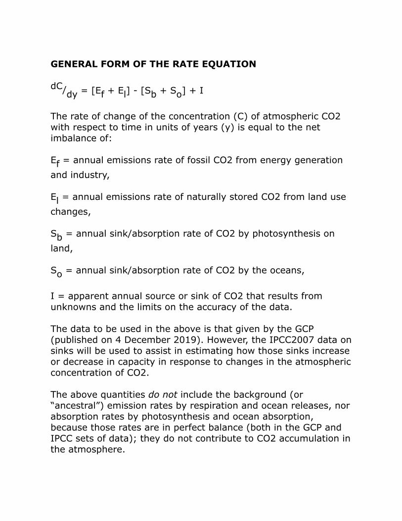
GENERAL FORM OF THE RATE EQUATION

dC/dy = [Ef + El] - [Sb + So] + I

The rate of change of the concentration (C) of atmospheric CO2 with respect to time in units of years (y) is equal to the net imbalance of:

Ef = annual emissions rate of fossil CO2 from energy generation

and industry,

El = annual emissions rate of naturally stored CO2 from land use

changes,

Sb = annual sink/absorption rate of CO2 by photosynthesis on

land,

So = annual sink/absorption rate of CO2 by the oceans,

I = apparent annual source or sink of CO2 that results from unknowns and the limits on the accuracy of the data.

The data to be used in the above is that given by the GCP (published on 4 December 2019). However, the IPCC2007 data on sinks will be used to assist in estimating how those sinks increase or decrease in capacity in response to changes in the atmospheric concentration of CO2.

The above quantities do not include the background (or “ancestral”) emission rates by respiration and ocean releases, nor absorption rates by photosynthesis and ocean absorption, because those rates are in perfect balance (both in the GCP and IPCC sets of data); they do not contribute to CO2 accumulation in the atmosphere.

SINKS

From GCP2019 data:

Sb = 1.47ppm/y

So = 1.10ppm/y

Therefore

S = Sb + So = 2.57ppm/y,

C = 407.4ppm at the end of 2018.

From IPCC2007 data:

Sb = 1.22ppm/y

So = 1.22ppm/y, (= 9.79-8.57, ppm/y)

Therefore

S = Sb + So = 2.44ppm/y,

C = 375ppm at the end of 2004.

The above shows a growth in the capacity of the total Sink (S) as the concentration was increased. This probably reflects an added stimulation for CO2 absorption by photosynthesis and the oceans because of an increased concentration of atmospheric CO2. Will this ‘growth of CO2 appetite effect’ be true indefinitely, or will this effect saturate at some higher level of CO2 concentration? Unknown (by me).

The simplest speculative quantification of this ‘sink growth’ effect that I can form is a linear relationship between S and C:

The slope of that linear equation is given by

∆S/∆C = (2.57-2.44, ppm/y)/(407.4-375, ppm) =

= 4.012*10-3 y-1 = (249.23y)-1,

so that S as a function of C is given by

S = [C-407.4, ppm]/249.23y + 2.57ppm/y.

This relationship gives:

S = 0.94 ppm/y at C = 0 ppmS = 2.05 ppm/y at C = 277 ppmS = 2.44 ppm/y at C = 375 ppmS = 2.57 ppm/y at C = 407.4 ppmS = 10.97 ppm/y at C = 2500 ppm.

In reality, I would expect S equal to 0 when C is zero, and to saturate at a capacity below 10.97ppm/y when C is at 2500ppm, or some as-yet to be reached high level of concentration. Nevertheless, I will use this model of sink capacity as a function of atmospheric CO2 concentration.

<><><><><><><>

The idea of linking S and C with a linear relationship was suggested to me (in a personal correspondence) by Sibbele Hietkamp, Chemist (PhD) who specialises in energy related science as well as energy efficiency and is living in South Africa. The linear relationship I use here is different from the one Sibbele Hietkamp is using. I have found his suggestions and corrections most helpful.

<><><><><><><>

LONG TERM CO2 SWEEPERS AND THE PETM

The “fast” processes, which initially scavenge atmospheric CO2, are photosynthesis and absorption by the oceans. Each of these processes can saturate if there is too much atmospheric CO2, and if the emission fluxes (both their magnitude and speed) are higher that the total sink capacity (scavenging rate).

The long-term, or “slow,” processes of scavenging atmospheric CO2 are the chemical reactions of weathering of rocks (carbonate and silicate) and soils.

Somewhere between 14,000GtCO2 and 26,000GtCO2 was injected into the atmosphere 55.5 million years ago (55.5mya) over a geologically short span of perhaps 1000 to 3000 years, most likely by a combination of volcanic activity, magmatic heating of seafloor carbonate sediments, wildfires and the burning of peat deposits. The time of this event is now classified by geologists as the transition from the Paleocene Epoch to the Eocene Epoch, and is known as the Paleocene-Eocene Thermal Maximum (PETM).

As noted by the PETM’s name, the Earth’s average global temperature reached its highest point since the extinction of the dinosaurs 66mya, during the 200,000 years of the PETM. After the relative cooling off of the PETM, the global temperature during the Eocene rose steadily for ~5my, peaking ~50mya at nearly the level of the highest temperature during the PETM excursion, and then fell steadily for ~15my, when the global temperature plummeted at the start of the Oligocene Epoch and Antarctic Glaciation began. The ~20my span after the PETM is known to geologists as the Eocene Optimum, a long period of high global temperature with an ice-free Earth; with swamps, ferns and Redwood forests in the Arctic, and jungles in the Antarctic.

I gave a detailed description of the PETM, and pointed out two major expositions on it (a 2014 video-recorded presentation by

Dr. Scott Wing of the Smithsonian Institute, and a major publication on Climate Change by the National Research Council of National Academies of Science in 2011), in the following report (at the web-link).

<><><><><><><>

Ye Cannot Swerve Me: Moby-Dick and Climate Change15 July 2019https://manuelgarciajr.com/2019/07/15/ye-cannot-swerve-me-moby-dick-and-climate-change/

<><><><><><><>

Note 11 from the above article is duplicated below.

<><><><><><><>

CO2 “lifetime” in the atmosphereNational Research Council 2011. Understanding Earth's Deep Past: Lessons for Our Climate Future. Washington, DC: The National Academies Press.Figure 3.5, page 93 of the PDF file, page numbered 78 in the text. https://doi.org/10.17226/13111

CO2 Sweepers and Sinks in the Earth SystemThe carbon fluxes in and out of the surface and sedimentary reservoirs over geological timescales are finely balanced, providing a planetary thermostat that regulates Earth’s surface temperature. Initially, newly released CO2 (e.g., from the combustion of hydrocarbons) interacts and equilibrates with Earth’s surface reservoirs of carbon on human timescales (decades to centuries). However, natural “sinks” for anthropogenic CO2 exist only on much longer timescales, and it is therefore possible to perturb climate for tens to hundreds of thousands of years (Figure 3.5). Transient (annual to century-scale) uptake by the terrestrial biosphere (including soils) is

easily saturated within decades of the CO2 increase, and therefore this component can switch from a sink to a source of atmospheric CO2 (Friedlingstein et al., 2006). Most (60 to 80 percent) CO2 is ultimately absorbed by the surface ocean, because of its efficiency as a sweeper of atmospheric CO2, and is neutralized by reactions with calcium carbonate in the deep sea at timescales of oceanic mixing (1,000 to 1,500 years). The ocean’s ability to sequester CO2 decreases as it is acidified and the oceanic carbon buffer is depleted. The remaining CO2 in the atmosphere is sufficient to impact climate for thousands of years longer while awaiting sweeping by the “ultimate” CO2 sink of the rock weathering cycle at timescales of tens to hundreds of thousands of years (Zeebe and Caldeira, 2008; Archer et al., 2009). Lessons from past hyperthermals suggest that the removal of greenhouse gases by weathering may be intensified in a warmer world but will still take more than 100,000 years to return to background values for an event the size of the Paleocene-Eocene Thermal Maximum (PETM).

In the context of the timescales of interaction with these carbon sinks, the mean lifetime of fossil fuel CO2 in the atmosphere is calculated to be 12,000 to 14,000 years (Archer et al., 1997, 2009), which is in marked contrast to the two to three orders of magnitude shorter lifetimes commonly cited by other studies (e.g., IPCC, 1995, 2001). In addition, the equilibration timescale for a pulse of CO2 emission to the atmosphere, such as the current release by fossil fuel burning, scales up with the magnitude of the CO2 release. “The result has been an erroneous conclusion, throughout much of the popular treatment of the issue of climate change, that global warming will be a century-timescale phenomenon” (Archer et al., 2009, p. 121).

<><><><><><><>

The “Figure 3.5” noted in the above excerpt from the 2011 NRC report is given here.

CO2 “lifetime” in the atmosphere.

It was because of the above that my earlier estimates of how long it would take to clear away the present excess of CO2 in the atmosphere, if we were to halt all anthropogenic emissions, range to about 1,300 years. The radiation of the excess heat-energy (which controls the weather) stored in the oceans would take longer.

I arrived at a mathematical function to characterize the long-term sweeping of atmospheric CO2, guided by the information given in the above reports, in the following manner.

A computer simulation of the PETM “instantly” injected over 18,000GtCO2 (5000GtC) into the atmosphere to arrive at a CO2 concentration of 2500ppm. Half of this atmospheric load of CO2 (carbon) was scavenged in the first 1000 years; 30% to 40% remained at 10,000 years; and “all” of that remainder was removed well after 100,000 years, mainly during the last 50,000 years of the entire 200,000 year span of the PETM. As noted by the 2011 NRC report, the lifetime of CO2 in the atmosphere is 12,000 to 14,000 years.

A very crude estimate of the average removal rate during the first 1000 years is

(2500-1250, ppm)/1000y = 1.25ppm/y.

The estimated concentration at 10,000 years is 875ppm (35% of 2500ppm). A very crude estimate of the removal rate during the subsequent 9,000 years is

(1250-875, ppm)/(10,000-1000, y) = 4.17*10-2 ppm/y.

A very crude estimate of the removal rate during the final 190,000 years of the PETM is

(875-275, ppm)/(200,000-10,000, y) = 3.16*10-3 ppm/y.

If the decay of CO2 concentration during the first 1000 years of the PETM was exponential, then it can be characterized by

C = C1*e-(y-y1)/1442.7y

, (at year “y” after year y1),

for C1 the initial concentration at y1 the start time (in years).

C=(C1/2) at (y-y1)=1000y.

The derivative of that decay function is

dC/dy = -(C1/1442.7y)*e-(y-y1)/1442.7y

.

For C1=2500ppm, this moderately long-term decay rate function

is

dC/dy = -(1.73)*e-(∆y)/1442.7y

ppm/y.

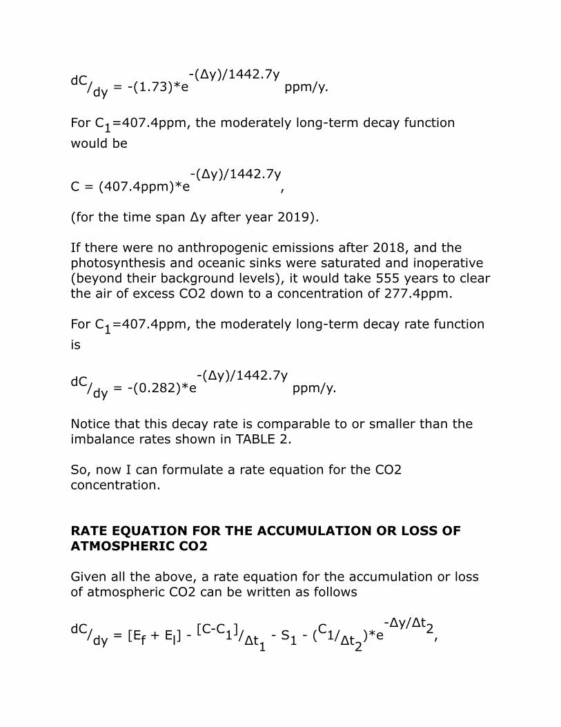
For C1=407.4ppm, the moderately long-term decay function

would be

C = (407.4ppm)*e-(∆y)/1442.7y

,

(for the time span ∆y after year 2019).

If there were no anthropogenic emissions after 2018, and the photosynthesis and oceanic sinks were saturated and inoperative (beyond their background levels), it would take 555 years to clear the air of excess CO2 down to a concentration of 277.4ppm.

For C1=407.4ppm, the moderately long-term decay rate function

is

dC/dy = -(0.282)*e-(∆y)/1442.7y

ppm/y.

Notice that this decay rate is comparable to or smaller than the imbalance rates shown in TABLE 2.

So, now I can formulate a rate equation for the CO2 concentration.

RATE EQUATION FOR THE ACCUMULATION OR LOSS OF ATMOSPHERIC CO2

Given all the above, a rate equation for the accumulation or loss of atmospheric CO2 can be written as follows

dC/dy = [Ef + El] - [C-C1]/∆t1

- S1 - (C1/∆t2)*e

-∆y/∆t2,

where:

∆t1 = 249.23y,

∆t2 = 1442.7y,

S1 = 2.57ppm/y,

and the other quantities are as previously defined (∆y is the elapsed time since the ‘starting’ year).

To solve this equation, I first substitute the variable name “x” for ∆y, the independent variable.

dC/dx = [Ef + El] - [C-C1]/∆t1

- S1 - (C1/∆t2)*e

-x/∆t2.

Two of the steps in the derivation of the solution are as follows:

dC/dx + (C/∆t1) = [Ef + El - S1 + C1/∆t1

] - (C1/∆t2)*e

-x/∆t2.

[e-x/∆t1]*d/dx[C*e

+x/∆t1] = [Ef + El - S1 + C1/∆t1] +

- (C1/∆t2)*e

-x/∆t2.

Integration of this last form yields

C(x) = C1*e-x/∆t1 + [(Ef + El - S1)*∆t1 + C1]*[1 - e

-x/∆t1] +

- [C1*e-x/∆t1]*[1 - e

-x/∆t2],

which simplifies to

C(x) = C1*e-x*[1/∆t1 + 1/∆t2]

+

+ [(Ef + El - S1)*∆t1 + C1]*[1 - e-x/∆t1].

This is the projected near-term time history for CO2 concentration C, given specific values for the parameters shown.

CASE #1

For “business as usual,” using the parameters at the end of year 2018:

C1 = 407.4ppm,

Ef = 4.28ppm/y,

El = 0.73ppm/y,

S1 = 2.57ppm/y,

∆t1 = 249.23y,

∆t2 = 1442.7y,

C(year “y”) = (407.4ppm)*e-(y-2019)/212.52y

+

+ (851.8ppm)*[1 - e-(y-2019)/249.52

].

This is a pure growth trend from 407.4ppm to 851.8ppm over the course of about 3,000 years.

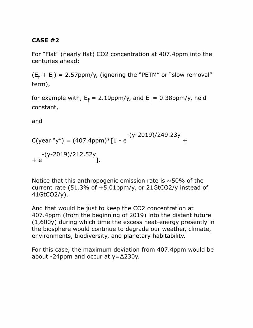
CASE #2

For “Flat” (nearly flat) CO2 concentration at 407.4ppm into the centuries ahead:

(Ef + El) = 2.57ppm/y, (ignoring the “PETM” or “slow removal”

term),

for example with, Ef = 2.19ppm/y, and El = 0.38ppm/y, held

constant,

and

C(year “y”) = (407.4ppm)*[1 - e-(y-2019)/249.23y

+

+ e-(y-2019)/212.52y

].

Notice that this anthropogenic emission rate is ~50% of the current rate (51.3% of +5.01ppm/y, or 21GtCO2/y instead of 41GtCO2/y).

And that would be just to keep the CO2 concentration at 407.4ppm (from the beginning of 2019) into the distant future (1,600y) during which time the excess heat-energy presently in the biosphere would continue to degrade our weather, climate, environments, biodiversity, and planetary habitability.

For this case, the maximum deviation from 407.4ppm would be about -24ppm and occur at y=∆230y.

CASE #3

To have dC/dx = 0 at C=0, in the rate equation, (so always have

C≥0),

we must have

[Ef + El] = S1 - (C1/∆t1)*[1 - (∆t1/∆t2

)*e-(∆y)/∆t2],

[Ef + El] = 2.57ppm/y - (1.63ppm/y)*[1 +

- (1/5.79)*e-(∆y)/1442.7y

].

Expecting this situation to be operative after ∆t1 = 249.23y, and

using that value for ∆y in the above, gives

[Ef + El] = 1.18ppm/y, (or 9.64GtCO2/y).

Notice that this anthropogenic emission rate is ~1/5 of the current total emission rate of 5.01ppm/y, or 41GtCO2/y.

Projections by the GCP are that anthropogenic emissions after 2019 will rise above 42GtCO2/y (or, +5.14ppm/y). Recall, it is unknown how much longer the growth of ‘CO2 appetite’ by the photosynthesis and oceanic sinks will continue.

The projected concentration history for this “maximum loss” case (from 407.4ppm to 60.97ppm, over the course of ~700+y) is

C(year “y”) = (407.4ppm)*e-(y-2019)/212.52y

+

+ (60.97ppm)*[1 - e-(y-2019)/249.23y

].

Again, recall that in the three cases above, I have allowed the photosynthesis and oceanic sinks (above background) to proportionally track the concentration (C) over its full range of values. This is an overly optimistic assumption. Were this ‘growth of CO2 appetite effect’ constrained to operate in a smaller range of concentration values, then the ‘clearing times’ that would be estimated, from cases similar to CASE #3, would be longer, probably stretching from centuries to millennia (with long-term weathering being the operative process).

Also, with sinks constrained to a smaller range of C values, CASE #1 will rise to higher concentrations sooner and the corresponding global temperature will also rise higher and sooner than would be calculated from the following.

TEMPERATURE RISE FOR “BUSINESS AS USUAL”

The projected history of temperature rise (from 2019) for “business as usual” (CASE #1) can be estimated as follows.

∆T in 2019, for 407.4ppm, was +1°C. The concentration that year was 130ppm above 277.4ppm, which I take as representative of pre-industrial conditions.

Therefore, ∆T for CASE #1 can be modeled as

∆T = +(1/130ppm)*{(407.4ppm)e-(∆y)/212.52y

+

+ (851.78ppm)*[1 - e-(∆y)/249.23

] - 277.4ppm},

in °C above the global temperature in pre-industrial times. Inserting the appropriate parametric values gives

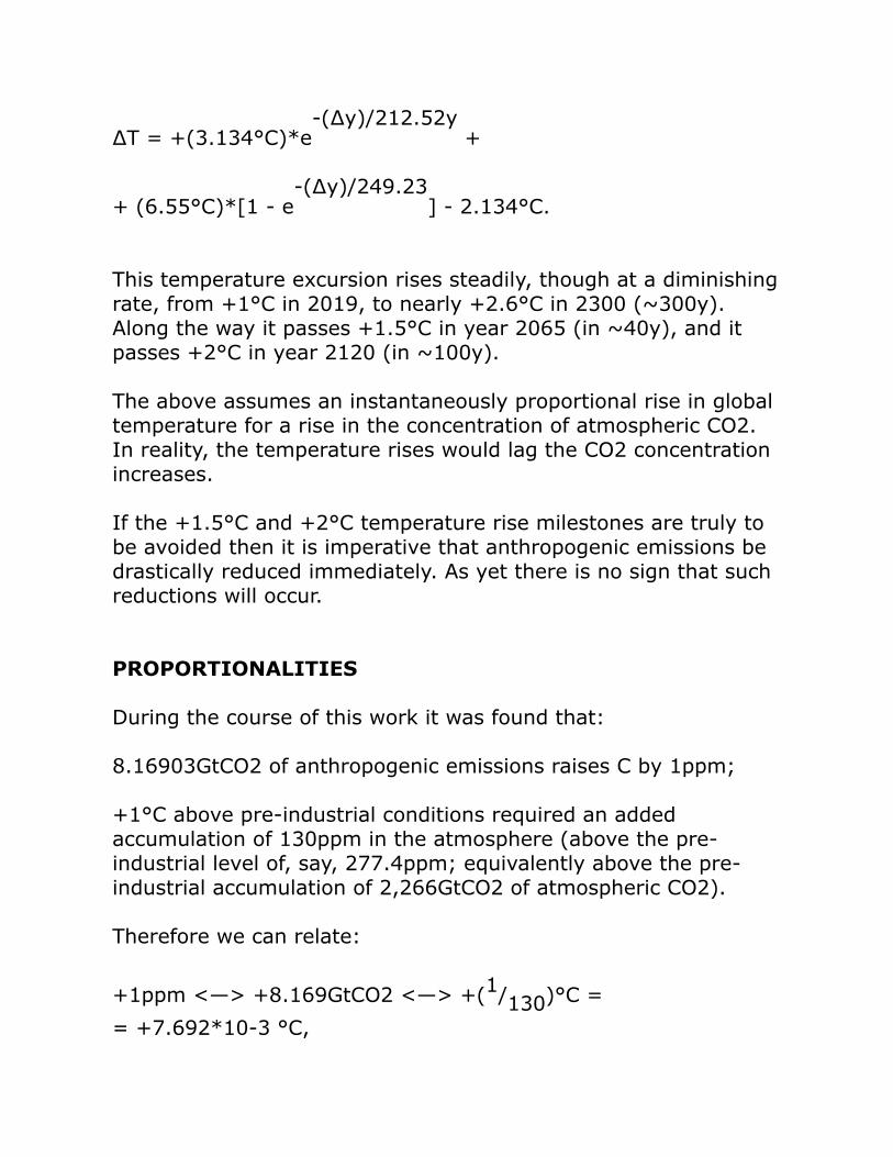
∆T = +(3.134°C)*e-(∆y)/212.52y

+

+ (6.55°C)*[1 - e-(∆y)/249.23

] - 2.134°C.

This temperature excursion rises steadily, though at a diminishing rate, from +1°C in 2019, to nearly +2.6°C in 2300 (~300y). Along the way it passes +1.5°C in year 2065 (in ~40y), and it passes +2°C in year 2120 (in ~100y).

The above assumes an instantaneously proportional rise in global temperature for a rise in the concentration of atmospheric CO2. In reality, the temperature rises would lag the CO2 concentration increases.

If the +1.5°C and +2°C temperature rise milestones are truly to be avoided then it is imperative that anthropogenic emissions be drastically reduced immediately. As yet there is no sign that such reductions will occur.

PROPORTIONALITIES

During the course of this work it was found that:

8.16903GtCO2 of anthropogenic emissions raises C by 1ppm;

+1°C above pre-industrial conditions required an added accumulation of 130ppm in the atmosphere (above the pre-industrial level of, say, 277.4ppm; equivalently above the pre-industrial accumulation of 2,266GtCO2 of atmospheric CO2).

Therefore we can relate:

+1ppm <—> +8.169GtCO2 <—> +(1/130)°C =

= +7.692*10-3 °C,

and

the addition of 1,061.97GtCO2 to the atmosphere raises the global temperature by +1°C.

GRAPHS

The following 5 graphs are shown:

CO2 ppm trend (2019-2300)

CO2 ppm trend (2019-2120)

CO2 ppm trend, “flat case” (2019-3600)

CO2 ppm trend, “PETM case” (2019-10,000)

“Business as Usual” temperature rise (2019-2200)

<><><><><><><>