A QUANTUM CHEMICAL STUDY OF TITANIUM DIOXIDE SURFACES

A QUANTUM CHEMICAL STUDY OF

WATER AND AMMONIA ADSORPTION MECHANISMS ON

TITANIUM DIOXIDE SURFACES

A THESIS SUBMITTED TO

THE GRADUATE SCHOOL OF NATURAL AND APPLIED SCIENCES OF

MIDDLE EAST TECHNICAL UNIVERSITY

BY

REZAN ERDOĞAN

IN PARTIAL FULFILLMENT OF THE REQUIREMENTS FOR

THE DEGREE OF MASTER OF SCIENCE IN

CHEMICAL ENGINEERING

JANUARY 2010

Approval of the thesis:

A QUANTUM CHEMICAL STUDY OF WATER AND AMMONIA ADSORPTION MECHANISMS ON TITANIUM DIOXIDE SURFACES

submitted by REZAN ERDOĞAN in partial fulfillment of the requirements for the degree of Master of Science in Chemical Engineering Department, Middle East Technical University by, Prof. Dr. Canan Özgen Dean, Graduate School of Natural and Applied Sciences Prof. Dr. Gürkan Karakaş Head of Department, Chemical Engineering Prof. Dr. Işık Önal Supervisor, Chemical Engineering Dept., METU Examining Committee Members: Prof. Dr. Hayrettin Yücel Chemical Engineering Dept., METU Prof. Dr. Işık Önal Chemical Engineering Dept., METU Prof. Dr. Güngör Gündüz Chemical Engineering Dept., METU Prof. Dr. Şinasi Ellialtıoğlu Physics Dept., METU Assoc. Prof. Dr. Göknur Bayram Chemical Engineering Dept., METU

Date: January 15, 2010

iii

I hereby declare that all information in this document has been obtained and presented in accordance with academic rules and ethical conduct. I also declare that, as required by these rules and conduct, I have fully cited and referenced all material and results that are not original to this work. Name, Last name : Rezan Erdoğan Signature :

iv

ABSTRACT

A QUANTUM CHEMICAL STUDY OF WATER AND AMMONIA ADSORPTION MECHANISMS ON

TITANIUM DIOXIDE SURFACES

Erdoğan, Rezan

M.Sc., Department of Chemical Engineering

Supervisor : Prof. Dr. Işık Önal

January 2010, 106 pages

Theoretical methods can be used to describe surface chemical reactions in detail

and with sufficient accuracy. Advances, especially in density functional theory

(DFT) method, enable to compare computational results with experiments.

Quantum chemical calculations employing ONIOM DFT/B3LYP/6-31G**-

MM/UFF cluster method provided in Gaussian 03 are conducted to investigate

water adsorption on rutile (110), and water and ammonia adsorption on anatase

(001) surfaces of titanium dioxide. Water and ammonia adsorption on anatase

(001) surface is studied by also performing PW:DFT-GGA-PW91 periodic DFT

method by using VASP code and the results are compared with the results of

ONIOM method.

v

The results obtained by means of ONIOM method indicate that dissociative water

adsorption on rutile (110) surface is not favorable due to high activation barrier,

whereas on anatase (001) surface, it is favorable since molecular and dissociative

water adsorption energies are calculated to be -23.9 kcal/mol and -58.12 kcal/mol.

Moreover, on anatase (001) surface, dissociative ammonia adsorption is found

energetically more favorable than molecular one (-37.17 kcal/mol vs. -23.28

kcal/mol). Thermodynamic functions at specific experimental temperatures for

water and ammonia adsorption reactions on anatase (001) surface are also

evaluated.

The results obtained using periodic DFT method concerning water adsorption on

anatase (001) surface indicate that dissociative adsorption is more favorable than

molecular one (-32.28 kcal/mol vs. -14.62 kcal/mol) as in ONIOM method. On

the same surface molecular ammonia adsorption energy is computed as -25.44

kcal/mol.

The vibration frequencies are also computed for optimized geometries of

adsorbed molecules. Finally, computed adsorption energy and vibration frequency

values are found comparable with the values reported in literature.

KEYWORDS: DFT; ONIOM; periodic DFT; rutile; water adsorption; anatase;

water and ammonia adsorption.

vi

ÖZ

SU VE AMONYAĞIN TİTANYUM DİOKSİT YÜZEYLERİ ÜZERİNDE

ADSORPSİYON MEKANİZMALARININ KUANTUM KİMYASAL

ÇALIŞMASI

Erdoğan, Rezan

Yüksek Lisans, Kimya Mühendisliği Bölümü

Tez Yöneticisi: Prof. Dr. Işık Önal

Ocak 2010, 106 sayfa

Kimyasal yüzey reaksiyonlarını ayrıntılı olarak ve yeterli doğrulukta tanımlamak

için teorik metotlar kullanılabilir. Özellikle ‘density functional theory’ (DFT)

metodundaki gelişmeler, hesaba dayalı sonuçları deneylerle karşılaştırmaya

olanak sağlar.

Titanyum dioksitin rutil (110) yüzeyi üzerinde su adsorpsiyonunu, anataz (001)

yüzeyi üzerinde su ve amonyak adsorpsiyonlarını incelemek için Gaussian 03

programında ONIOM DFT/B3LYP/6-31G**-MM/UFF küme metodu

kullanılarak kuantum kimyasal hesaplamalar yapılmıştır. Ayrıca, anataz (001)

yüzeyi üzerinde su ve amonyak adsorpsiyonları VASP kodu kullanılarak

PW:DFT-GGA-PW91 periyodik DFT metoduyla da çalışılmış ve sonuçlar

ONIOM metodunun sonuçlarıyla karşılaştırılmıştır.

vii

ONIOM metodu kullanılarak elde edilen sonuçlar, rutil (110) yüzeyi üzerinde

suyun ayrışma adsorpsiyonunun yüksek aktivasyon bariyerinden dolayı avantajlı

olmadığını, bununla birlikte anataz (001) yüzeyi üzerinde, suyun molekül olarak

ve ayrışarak gerçekleşen adsorpsiyon enerjileri -23.9 kcal/mol ve -58.12 kcal/mol

olarak hesaplandığından, suyun ayrışma adsorpsiyonunun molekül olarak

gerçekleşen su adsorpsiyonuna göre daha avantajlı olduğunu göstermektedir.

Ayrıca, anataz (001) yüzeyi üzerinde amonyağın ayrışma adsorpsiyonunun

molekül olarak gerçekleşen amonyak adsorpsiyonundan enerjiler açısından daha

avantajlı olduğu bulunmuştur. (-37.17 kcal/mol’e karşın -23.28 kcal/mol). Anataz

(001) yüzeyi üzerinde su ve amonyak adsorpsiyon reaksiyonları için belirli

deneysel sıcaklıklarda termodinamik fonksiyonlar da hesaplanmıştır.

Periyodik DFT metodu kullanılarak, anataz (001) yüzeyi üzerinde su

adsorpsiyonuna dair elde edilen sonuçlar, ONIOM metodunda olduğu gibi, suyun

ayrışma adsorpsiyonunun molekül olarak gerçekleşen su adsorpsiyonundan

enerjiler açısından daha avantajlı olduğunu işaret etmektedir (-32.28 kcal/mol’e

karşın -14.62 kcal/mol). Aynı yüzey üzerinde, moleküler olarak gerçekleşen

amonyak adsorpsiyonunun enerjisi -25.44 kcal/mol olarak bulunmuştur.

Adsorplanmış moleküllerin optimize edilmiş geometrilerinin vibrasyon frekans

değerleri de hesaplanmıştır. Son olarak, adsorpsiyon enerji ve vibrasyon frekans

değerlerinin literatürde belirtilen değerlerle kıyaslanabilir olduğu bulunmuştur.

ANAHTAR SÖZCÜKLER: DFT; ONIOM; periyodik DFT; rutil; su

adsorpsiyonu; anataz; su ve amonyak adsorpsiyonları.

viii

To my mother Filiz Erdoğan

ix

ACKNOWLEDGEMENTS

I wish to express my sincere thanks to my supervisor Prof. Dr. Işık Önal for his

guidance and interest throughout this study.

I would like to thank my colleague Dr. M. Ferdi Fellah for his helps, suggestions,

solutions to my problems, and conveying his invaluable experiences to me. I wish

also thank my colleague Oluş Özbek for his helps and criticism in periodic DFT

calculations using VASP. Thanks also to all my lab mates for their helpful and

enjoyable friendships throughout this study.

I would like to thank also my dear friend Volkan Çankaya for not only editing the

whole thesis with me but also his endless support and understanding.

This research was supported in part by TÜBİTAK through TR-Grid e-

Infrastructure Project. TR-Grid systems are hosted by TÜBİTAK ULAKBİM and

Middle East Technical University. Visit http://www.grid.org.tr for more

information.

x

TABLE OF CONTENTS

ABSTRACT................................................................................................................ iv

ÖZ ............................................................................................................................... vi

ACKNOWLEDGEMENTS........................................................................................ ix

TABLE OF CONTENTS............................................................................................. x

LIST OF TABLES.................................................................................................... xiii

LIST OF FIGURES .................................................................................................. xvi

LIST OF SYMBOLS AND ABBREVIATIONS ..................................................... xix

CHAPTERS

1. INTRODUCTION ...................................................................................................1

2. LITERATURE SURVEY........................................................................................9

2.1 Water Adsorption on Rutile TiO2 (110) Surface................................................9

2.1.1 Experimental Studies.................................................................................9

2.1.2 Theoretical Studies ..................................................................................10

2.2 Water and Ammonia Adsorption on Anatase TiO2 (001) Surface...................12

2.2.1 Experimental Studies...............................................................................12

2.2.2 Theoretical Studies ..................................................................................13

3. METHODOLOGY ................................................................................................16

3.1 Overview of Computational Quantum Chemistry ...........................................16

xi

3.2 ONIOM Method...............................................................................................19

3.3 Surface Models and Computational Methods ..................................................23

3.3.1 ONIOM Cluster Method..........................................................................24

3.3.1.1 Surface Models.....................................................................................24

3.3.1.2 Computational Method.........................................................................32

3.3.2 Periodic DFT Method..............................................................................34

3.3.2.1 Surface Model and Computational Method .........................................34

4. RESULTS AND DISCUSSION............................................................................36

4.1 ONIOM Cluster Method ..................................................................................36

4.1.1 Water Adsorption on Rutile TiO2 (110) Cluster Surface ........................36

4.1.1.1 Optimization of Cluster ........................................................................36

4.1.1.2 Molecular Adsorption Mechanism.......................................................38

4.1.1.3 Dissociative Adsorption Mechanism....................................................39

4.1.1.4 Comparison of Adsorption Energies with Literature Values ...............41

4.1.1.5 Vibrational Frequency Studies .............................................................43

4.1.2 Water and Ammonia Adsorption on Anatase TiO2 (001) Cluster

Surface..............................................................................................................45

4.1.2.1 Optimization of Cluster ........................................................................45

4.1.2.2 Water Adsorption on Anatase TiO2 (001) Cluster Surface ..................46

4.1.2.2.1 Molecular Adsorption Mechanism....................................................46

4.1.2.2.2 Dissociative Adsorption Mechanism.................................................47

4.1.2.2.3 Comparison of Adsorption Energies with Literature Values ............48

4.1.2.2.4 Vibrational Frequency Studies ..........................................................49

4.1.2.2.5 Thermochemical Data at Specific Temperatures ..............................49

4.1.2.3 Ammonia Adsorption on Anatase TiO2 (001) Cluster Surface ............51

xii





4.1.2.3.5 Thermochemical Data at Specific Temperatures ..............................57

4.2 Periodic DFT Method ......................................................................................59

4.2.1 Water and Ammonia Adsorption on Anatase TiO2 (001) Slab Surface..59

4.2.1.1 Optimization of Slab Geometry............................................................59

4.2.1.2 Water Adsorption on Anatase TiO2 (001) Slab Surface.......................60





4.2.1.3 Ammonia Adsorption on Anatase TiO2 (001) Slab Surface ................64




5. CONCLUSIONS....................................................................................................67

REFERENCES ..........................................................................................................69

APPENDICES

A. BACKGROUND AND THEORY OF COMPUTATIONAL QUANTUM

CHEMISTRY ............................................................................................................78

B. SAMPLE INPUT AND OUTPUT FILES ............................................................84

xiii

LIST OF TABLES

TABLES

Table 1.1 Gregor's analysis of the ilmenite............................................................2

Table 1.2 Bulk properties of TiO2 (rutile) .............................................................3

Table 3.1 Experimental parameters of TiO2 (Rutile)...........................................24

Table 3.2 Atomic parameters (Fractional coordinates) of TiO2 (Rutile) .............24

Table 3.3 Atomic parameters (Cartesian coordinates) of TiO2 (Rutile) ..............25

Table 3.4 Experimental parameters of TiO2 (Anatase)........................................28

Table 3.5 Atomic parameters (Fractional coordinates) of TiO2 (Anatase) ..........28

Table 3.6 Atomic parameters (Cartesian coordinates) of TiO2 (Anatase) ...........29

Table 4.1 The comparison of the atomic displacements away from the

rutile TiO2 (110) surface relative to an ideal bulk structure with

the available literature values................................................................37

Table 4.2 The comparison of the calculated energies of H2O adsorption

and activation barrier on rutile TiO2 (110) surface with the

theoretical and experimental values in the literature.............................42

Table 4.3 Structural and vibrational properties of adsorbed H2O molecule

(molecularly and dissociatively) on rutile TiO2 (110) surface via

ONIOM DFT/B3LYP/6-31G**-MD/UFF calculations c .....................44

xiv

Table 4.4 A comparison of the calculated H2O adsorption energies

(kcal/mol) on perfect anatase TiO2 (001) surface with the


Table 4.5 Vibrational frequencies (cm-1) of dissociatively adsorbed H2O

molecule on anatase TiO2 (001) surface as obtained from

ONIOM DFT/B3LYP-6-31G**-MD/UFF calculations. ......................49

Table 4.6 Calculated ΔH˚, ΔG˚ (kcal/mol), and ΔS˚ (cal/mol.K) values at

0 K and specific experimental temperatures (170, 260 K) [52]

for H2O adsorption on anatase TiO2 (001) surface b .............................50

Table 4.7 A comparison of the calculated NH3 adsorption energies on

anatase TiO2 (001) surface with the theoretical and experimental

values in the literature ...........................................................................55

Table 4.8 The vibrational frequency (cm-1) properties of molecularly and

dissociatively adsorbed NH3 molecule on anatase TiO2 (001)

surface as obtained from ONIOM DFT/B3LYP-MD/UFF

calculations with the experimental literature values e ...........................56

Table 4.9 Calculated ΔH˚, ΔG˚ (kcal/mol), and ΔS˚ (cal/mol.K) values at

0 K and specific experimental temperatures (150, 360 K [52],

and 423 K [59]) for NH3 adsorption on anatase TiO2 (001)

surface c .................................................................................................58

Table 4.10 A comparison of the calculated H2O adsorption energies

(kcal/mol) on perfect anatase TiO2 (001) surface with the


Table 4.11 Vibrational frequencies (cm-1) of dissociatively adsorbed H2O

molecule on anatase TiO2 (001) surface as obtained from

periodic DFT (PW:DFT-GGA) calculations.........................................63

xv

Table 4.12 A comparison of the calculated NH3 adsorption energies on

perfect anatase TiO2 (001) surface with the theoretical and

experimental values in the literature .....................................................65

Table 4.13 A comparison of the vibrational frequencies (cm-1) of

molecularly adsorbed NH3 molecule on anatase TiO2 (001)

surface as obtained from periodic DFT (PW:DFT-GGA)

calculations with the experimental literature values e ...........................66

Table B.1 Gaussian input file of vibrational frequency calculation of

optimized single H2O molecule ............................................................85

Table B.2 Gaussian output file of vibrational frequency calculation of

optimized single H2O molecule. ...........................................................86

Table B.3 Gaussian input file for coordinate driving calculation of

dissociative NH3 adsorption on anatase TiO2 (001) surface. ................95

Table B.4 Gaussian input file for transition state calculation of

dissociative NH3 adsorption on anatase TiO2 (001) surface .................98

Table B.5 VASP files (POSCAR, INCAR, K-POINTS, and POTCAR) for

volume relaxation calculation of anatase TiO2. ..................................105

xvi

LIST OF FIGURES

FIGURES

Figure 1.1 TiO2 crystals (titanium white) ..............................................................1

Figure 1.2 Observed conditions for persistence or induced transformation

of unstable anatase [7].............................................................................4

Figure 1.3 Observed conditions for persistence or induced transformation

of unstable brookite [7]. ..........................................................................4

Figure 1.4 Bulk structures of rutile and anatase. The tetragonal bulk unit

cell of rutile has the dimensions, a=b=4.587 Å, c=2.953 Å, and

the one of anatase a=b=3.782 Å, c=9.502 Å [4].. ...................................5

Figure 1.5 The equilibrium shape of a macroscopic TiO2-rutile crystal

using the Wulff construction and surface energies calculated in

[8] ............................................................................................................6

Figure 1.6 (a) The equilibrium shape of a TiO2-anatase crystal according

to the Wulff construction and surface energies calculated in [17].

(b) Picture of an anatase mineral crystal .................................................7

Figure 3.1 A comparison of the computational quantum chemistry models

in terms of accuracy and computational cost. .......................................19

Figure 3.2 ONIOM terminology for link atoms using ethane [76]......................22

Figure 3.3 (a) TiO2 (rutile) unit cell (Ti2O4). (b) The completed tetragonal

cell (Ti9O6) ............................................................................................25

xvii

Figure 3.4 The 3-D structures of enlarged (3x-3y-3z) TiO2 (rutile) cluster ........26

Figure 3.5 (a) TiO2 Rutile (110) cluster surface. (b) ONIOM TiO2 Rutile

(110) cluster surface. .............................................................................27

Figure 3.6 (a) TiO2 (anatase) unit cell (Ti2O4). (b) The completed

tetragonal cell (Ti11O18).........................................................................29

Figure 3.7 The 3-D structures of enlarged (3x-3y-1z) TiO2 (anatase)

cluster ....................................................................................................30

Figure 3.8 (a) TiO2 Anatase (001) cluster surface. (b) ONIOM TiO2

Anatase (001) cluster surface. ...............................................................31

Figure 3.9 Four layer p(2x2) TiO2 anatase (001) slab .........................................34

Figure 4.1 Optimized geometry of 2-region ONIOM rutile TiO2 (110)

cluster model .........................................................................................36

Figure 4.2 Relative energy profile and equilibrium geometry of molecular

H2O adsorption on rutile TiO2 (110) surface. .......................................38

Figure 4.3 Relative energy profile for dissociative H2O adsorption on

rutile TiO2 (110) surface. ......................................................................39

Figure 4.4 Dissociative H2O adsorption on rutile TiO2 (110) surface.

(a) Equilibrium geometry, (b) Transition state geometry .....................40

Figure 4.5 Relative energy diagram of reaction steps of molecular and

dissociative H2O adsorption on rutile TiO2 (110) surface ....................41

Figure 4.6 Optimized geometry of 2-region ONIOM anatase TiO2 (001)

cluster model .........................................................................................45

Figure 4.7 Relative energy profile for the adsorption of single water

molecule on (001) anatase TiO2 surface................................................46

xviii

Figure 4.8 (a) Molecular H2O adsorption geometry on anatase TiO2 (001)

surface. (b) Equilibrium geometry of dissociative H2O

adsorption on anatase TiO2 (001) surface. ............................................47

Figure 4.9 Relative energy profile and equilibrium geometry of molecular

NH3 adsorption on anatase TiO2 (001) surface. ....................................51

Figure 4.10 Relative energy profile for dissociative NH3 adsorption on

anatase TiO2 (001) surface ....................................................................52

Figure 4.11 Geometries of dissociative NH3 adsorption on anatase TiO2

(001) surface. (a) Equilibrium geometry, (b) Transition state

geometry................................................................................................53

Figure 4.12 A summary energy diagram of molecular and dissociative

NH3 adsorption on anatase TiO2 (001) surface .....................................54

Figure 4.13 Optimized slab geometry of 4 layer p(2x2) TiO2 anatase (001)

slab ........................................................................................................59

Figure 4.14 Optimized geometry of molecular H2O adsorption on anatase

TiO2 (001) slab model. (a) Perspective view, (b) Top view..................60

Figure 4.15 Optimized geometry of dissociative H2O adsorption on

anatase TiO2 (001) slab model. (a) Perspective view, (b) Top

view.......................................................................................................61

Figure 4.16 Optimized geometry of molecular NH3 adsorption on anatase

TiO2 (001) slab model. (a) Perspective view, (b) Top view..................64

xix

LIST OF SYMBOLS AND ABBREVATIONS

CI 77891 : Color index number for TiO2

E171 : E number (food additive) for TiO2

MOSFET : Metal oxide semiconductor field effect transistor

TPD : Temperature programmed desorption

XPS : X-ray photoelectron spectroscopy

HREELS : High resolution electron energy loss spectroscopy

UHV : Ultra high vacuum

STM : Scanning tunneling microscope

DFT : Density functional theory

HF : Hartree Fock

MP2 : Møller Plesset perturbation theory 2

PW91 : Perdew Wang 1991 functional

PBE : Perdew Burke Ernzerhof functional

FTIR : Fourier transform infrared

MO : Molecular orbital

SINDO1 : Semi-empirical MO

MSINDO : Semi-empirical molecular orbital

MSINDO-CCM : Semi-empirical molecular orbital method-cyclic cluster

model

CPU : Central processing unit

MM : Molecular mechanics

ONIOM : Our own n-layered integrated molecular orbital and

molecular mechanics

SM : Small model

IM : Intermediate model

R : Real

xx

B3LYP : Becke’s three-parameter hybrid method involving the Lee

et al. correlation functional formalism

QST3 : Synchronous quasi-Newtonian method of optimization

XRD : X-ray diffraction

BET : Brunauer et al. 1938

VASP : Vienna ab initio simulation package

PAW : Projector augmented-wave

GGA : Generalized gradient approximation

LDA : Local density approximation

LCAO : Linear combination of atomic orbital

RPBE : Revised Perdew Burke Ernzerhof functional

1

CHAPTER 1

INTRODUCTION

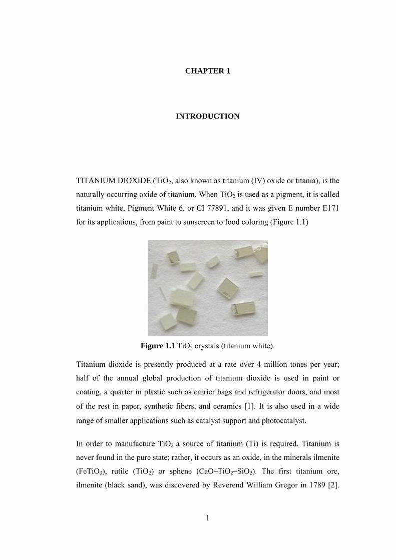
TITANIUM DIOXIDE (TiO2, also known as titanium (IV) oxide or titania), is the

naturally occurring oxide of titanium. When TiO2 is used as a pigment, it is called

titanium white, Pigment White 6, or CI 77891, and it was given E number E171

for its applications, from paint to sunscreen to food coloring (Figure 1.1)

Figure 1.1 TiO2 crystals (titanium white).

Titanium dioxide is presently produced at a rate over 4 million tones per year;

half of the annual global production of titanium dioxide is used in paint or

coating, a quarter in plastic such as carrier bags and refrigerator doors, and most

of the rest in paper, synthetic fibers, and ceramics [1]. It is also used in a wide

range of smaller applications such as catalyst support and photocatalyst.

In order to manufacture TiO2 a source of titanium (Ti) is required. Titanium is

never found in the pure state; rather, it occurs as an oxide, in the minerals ilmenite

(FeTiO3), rutile (TiO2) or sphene (CaO–TiO2–SiO2). The first titanium ore,

ilmenite (black sand), was discovered by Reverend William Gregor in 1789 [2].

2

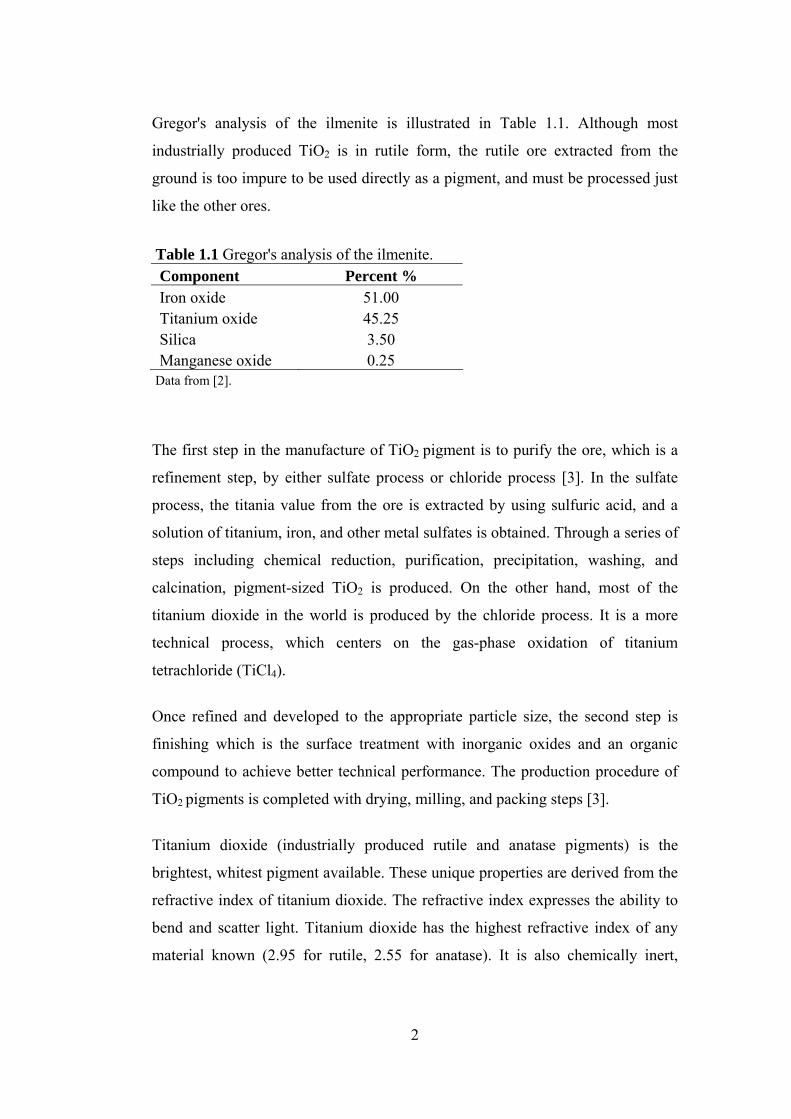
Gregor's analysis of the ilmenite is illustrated in Table 1.1. Although most

industrially produced TiO2 is in rutile form, the rutile ore extracted from the

ground is too impure to be used directly as a pigment, and must be processed just

like the other ores.

Table 1.1 Gregor's analysis of the ilmenite. Component Percent % Iron oxide 51.00 Titanium oxide 45.25 Silica 3.50 Manganese oxide 0.25

Data from [2].

The first step in the manufacture of TiO2 pigment is to purify the ore, which is a

refinement step, by either sulfate process or chloride process [3]. In the sulfate

process, the titania value from the ore is extracted by using sulfuric acid, and a

solution of titanium, iron, and other metal sulfates is obtained. Through a series of

steps including chemical reduction, purification, precipitation, washing, and

calcination, pigment-sized TiO2 is produced. On the other hand, most of the

titanium dioxide in the world is produced by the chloride process. It is a more

technical process, which centers on the gas-phase oxidation of titanium

tetrachloride (TiCl4).

Once refined and developed to the appropriate particle size, the second step is

finishing which is the surface treatment with inorganic oxides and an organic

compound to achieve better technical performance. The production procedure of

TiO2 pigments is completed with drying, milling, and packing steps [3].

Titanium dioxide (industrially produced rutile and anatase pigments) is the

brightest, whitest pigment available. These unique properties are derived from the

refractive index of titanium dioxide. The refractive index expresses the ability to

bend and scatter light. Titanium dioxide has the highest refractive index of any

material known (2.95 for rutile, 2.55 for anatase). It is also chemically inert,

3

insoluble in polymers, and heat stable under harshest processing conditions. It has

also high band gap energy (3.0 eV for rutile, 3.2 eV for anatase) [4].

Due to mixed ionic and covalent bonding in metal oxide systems, the surface

structure has a strong influence on local surface chemistry [5]. The bulk

properties of TiO2 (rutile) can be seen in Table 1.2.

Data from [5].

The surface of TiO2 is saturated by coordinatively bonded water, which then

forms hydroxyl ions. Depending on the type of bonding of the hydroxyl groups,

TiO2 shows acidic or basic character. The surface of TiO2 is thus always polar.

The presence of hydroxyl groups makes photochemically induced reactions

possible, e.g., the decomposition of water into hydrogen and oxygen and nitrogen

into ammonia and hydrazine (N2H4) [6].

Five polymorphs (crystalline forms) of TiO2 exist: anatase and brookite, which

are low-temperature, low-pressure forms; TiO2-II and TiO2-III, which are formed

from anatase or brookite under pressure; and rutile, the stable phase at all

temperature and ambient pressure [6].

The polymorphic transformations anatase to rutile and brookite to rutile do not

occur reversibly. This fact and heat of transformation data show that anatase and

brookite are not stable at any temperature. Similarly, the transformations of

anatase and brookite to the high-pressure forms, TiO2-II and TiO2-III, occur

irreversibly. The transformations of anatase → rutile, anatase → TiO2-II, and

TiO2-II → rutile in a nonequilibrium temperature-pressure diagram is shown in

Table 1.2 Bulk properties of TiO2 (rutile). Atomic radius (nm)

O (covalent) 0.066 Ti (metallic) 0.146 Ionic radius (nm) O (-2) 0.140 Ti (+4) 0.064

4

Figure 1.2. The transformations of brookite → rutile, brookite → TiO2-II, and

TiO2-II → rutile in a nonequilibrium temperature-pressure diagram can be seen in

Figure 1.3 [7].

Figure 1.2 Observed conditions for persistence or induced transformation of unstable anatase [7].

Figure 1.3 Observed conditions for persistence or induced transformation of unstable brookite [7].

5

The diagrams in Figures 1.2 and 1.3 indicate conditions for which the rate of

transformation in the appropriate direction is appreciable. Of the high-pressure

phases, TiO2-II is formed more easily and the only one that can be retained during

quenching. The transformation of anatase → rutile occurs infinitely slowly at 610

˚C. Transformation of rutile to TiO2-II occurs at pressures above 7 GPa and

temperatures above 700 ˚C. The transformation of TiO2-II to TiO2-III occurs at

about 20 to 30 GPa [7].

Among the crystalline forms of titania, rutile and anatase have given importance

since they play any role in the applications of TiO2. Their unit cells are shown in

Figure 1.4.

Figure 1.4 Bulk structures of rutile and anatase. The tetragonal bulk unit cell of rutile has the dimensions, a=b=4.587 Å, c=2.953 Å, and the one of anatase a=b=3.782 Å, c=9.502 Å [4].

6

In both rutile and anatase phases, the basic building block consists of a titanium

atom in the lattice surrounded octahedrally by six oxygen atoms and each oxygen

atom surrounded by three titanium atoms in trigonal arrangement.

Rutile, which is the most thermodynamically stable one, has the highest density

and the most compact atomic structure [6]. Many surface science studies focused

on single crystal rutile TiO2 (110) surface, because of its thermodynamic stability

and relatively easy preparation as a model surface [4]. Ramamoorthy and

Vanderbilt [8] calculated the total energy of periodic TiO2 slabs using a self-

consistent ab-initio method and they found that the (110) surface has the lowest

surface energy, and the (001) surface has the highest. From the calculated

energies, they constructed a three-dimensional Wulff plot, which gives the

equilibrium crystal shape of a macroscopic crystal, is shown in Figure 1.5.

Figure 1.5 The equilibrium shape of a macroscopic TiO2-rutile crystal using the Wulff construction [8].

Most commercial titania powder catalysts are a mixture of rutile and anatase (e.g.,

the most often used Degussa P25 contains approx. 80–90% anatase and the rest

rutile [9]). Such mixtures work best for certain photocatalytic reactions and non-

photo induced catalysis [10].

7

There is growing evidence that anatase is more active than rutile, especially in

catalysis, anatase phase of titanium dioxide is used much more often as a support

or a catalyst by itself [4,11,12].

TiO2-anatase nanoparticles have predominantly (101) and (100)/(010) majority

surfaces, together with minority (001) surface [13]. However, many studies

concerning the structure and reactivity of different anatase surfaces suggest that

the minority (001) surface is more reactive and plays a key role in the reactivity

of anatase nanoparticles [13-16]. The calculated Wulff shape of an anatase crystal

and the shape of naturally grown mineral samples can be seen in Figure 1.6.

Figure 1.6 (a) The equilibrium shape of a TiO2-anatase crystal according to the Wulff construction [17]. (b) Picture of an anatase mineral crystal.

TiO2 has wide range of technological applications. It is used in heterogeneous

catalysis (metal/TiO2 systems) [9,18], as a photocatalyst, in solar cells for the

production of hydrogen and electric energy [19], as a gas sensor [20], as a white

pigment (e.g. in paint, food, and cosmetic products) [21,22,23], as a corrosion-

protective coating [24], as an optical coating [25], in ceramics, and in electric

devices such as varistors [26]. It is used also in toxic material conversion [27,28]

and bone implants [29], air purifying, and self-cleaning window [30] applications.

It is utilized as a gate insulator for the new generation of MOSFETS (metal oxide

semiconductor field effect transistor) [31], as a spacer material in magnetic spin-

valve systems [32,33], and finds applications in nanostructured form in Li-based

batteries and electrochromic devices [34].

8

One good reason for pursuing research on single-crystalline TiO2 surfaces is that

it is a model system in surface science studies of metal oxides. The

thermodynamically stable rutile (110) surface certainly falls into this category.

Furthermore, TiO2 is a preferred system for experimentalists because it is well

suited for many experimental techniques. A second reason for studying TiO2

surfaces is the wide range of its applications in many fields including catalysis.

Water commands a fundamental interest as an adsorbate on TiO2 surfaces. To

illustrate, many of the applications, almost all photocatalytic processes, are

performed in an aqueous environment. In addition, TiO2 exposed to air will

always be covered by a water film and the presence of water can affect adsorption

and reaction processes. The adsorption of water on TiO2 have been extensively

reported both in experimental and theoretical literature. Therefore, in this study,

H2O adsorption on rutile and anatase TiO2 surfaces is studied to check the

reliability of the methodology used. In other words, this is a validation test for

future calculations on ammonia adsorption. NH3 adsorption on anatase TiO2 can

be important for industrial catalytic reactions such as selective catalytic reduction

(SCR) of NO and photo-oxidation of NH3 over TiO2. There are very few

experimental studies and theoretical calculations concerning adsorption of

ammonia on anatase TiO2. Moreover, for H2O and NH3 adsorptions on anatase

TiO2 surface, theoretical ONIOM and periodic DFT methods are intended to be

compared. It is known that periodic DFT methods involve heavy computations

but they are also more accurate methods.

The aim of this thesis is to theoretically investigate adsorption mechanisms of

H2O and NH3 molecules on different titania surfaces by using quantum chemical

calculations. More precisely, water adsorption on rutile TiO2 (110) surface is

studied by ONIOM method, water adsorption on anatase TiO2 (001) surface is

studied and compared by both ONIOM and periodic DFT methods, and finally

ammonia adsorption on anatase TiO2 (001) surface is studied and compared by

both ONIOM and periodic DFT methods.

9

CHAPTER 2

LITERATURE SURVEY

2.1 Water Adsorption on Rutile TiO2 (110) Surface

2.1.1 Experimental Studies

There are some experimental studies with regard to the surface properties and

adsorption mechanisms of water on rutile TiO2 (110) surface. Using synchrotron

radiation and photoemission spectroscopy Kurtz et al. [35] reported that water

molecules adsorbed on the perfect (stoichiometric) rutile (110) surface

molecularly or dissociatively depending on temperature.

Hugenshmith et al. [36] studied interaction of H2O with rutile TiO2 (110) surface

by TPD (temperature programmed desorption), XPS (x-ray photoelectron

spectroscopy) and work function measurements. They reported that water is

mainly molecularly adsorbed and not dissociated on this surface.

Henderson et al. [37] reached the same results as Hugenshmith et al. by

performing HREELS (high resolution electron energy loss spectroscopy) and

TPD studies. Henderson et al. [37] reported that water adsorbed on rutile TiO2

(110) surface predominately in a molecular state with exothermic adsorption

energy of 17-19 kcal/mol, little or no water dissociates on ideal TiO2 (110)

surface under UHV (ultra high vacuum) conditions; but that dissociation may be

linked to structural and/or point defects.

Brinkley et al. [38] investigated the adsorption properties of water on rutile TiO2

(110) surface using modulated molecular beam scattering and TPD studies. They

10

detected that very few of the molecules dissociate, even in the limit of zero

coverage and they found molecularly adsorbed H2O with -(17–24) kcal/mol

which is also in agreement with TPD studies reported in [36,37].

Recent STM (scanning tunneling microscope) studies, most notably the ones

published by Brookes et al. [39] and Schaub et al. [40] support the earlier

experimental results that dissociative adsorption occurs at defects or at oxygen

vacancies as active sites for water dissociation. Molecular adsorption is more

favorable than dissociation on the defect-free surface.

2.1.2 Theoretical Studies

There are many theoretical studies about adsorption reactions and surface

properties on rutile TiO2 (110). Unlike the experimental results, Goniakowski et

al. [41] found that dissociative adsorption of water molecule is

thermodynamically more stable than molecular adsorption with 6 kcal/mol lower

in adsorption energy.

Lindan et al. [42] also indicated that dissociation of the water molecule is

thermodynamically favored on low coverages but both molecular and dissociative

adsorption were confirmed at high coverages on rutile TiO2 (110) surface by use

of both DFT (density functional theory) and HF (Hartree-Fock) methods.

Casarin et al. [43] and Stefanovich et al. [44] predicted that molecular water

adsorption is more favorable than dissociative chemisorption as shown in recent

experimental studies. Casarin et al. [43] studied molecular adsorption of water on

rutile TiO2 (110) surface by use of DFT calculations and obtained -19.3 kcal/mol

molecular adsorption energy that in good agreement with experimental data.

Stefanovich et al. [44] have studied adsorption of a single water molecule in both

molecular and dissociative geometries by using HF, MP2 (Møller–Plesset

perturbation theory 2), and DFT/B3LYP methods. They concluded that isolated

11

water molecule adsorbs on the rutile TiO2 (110) surface in the molecular form and

adsorption energy was estimated to be about -30 kcal/mol.

Menetrey et al. [45] performed periodic DFT calculations to study the effect of

oxygen vacancies. They found that the reactivity at reduced surface differs from

that on the stoichiometric perfect surfaces. For the water molecule, the

dissociative adsorption energy (-31.6 kcal/mol) is lower than on the perfect

surface (-29.3 kcal/mol).

Most recent plane wave (PW:DFT-GGA-PW91) calculations performed by

Bandura et al. [46] pointed out that adsorption energy values for molecular and

dissociative adsorption of water molecule on rutile TiO2 (110) surface are -21.9

kcal/mol and -18.4 kcal/mol, respectively. They also employed ab-initio

(LCAO:HF LANL1-CEP) calculations on the same surface and reported that

molecular and dissociative adsorption energies of water are -22.5 kcal/mol and -

11.5 kcal/mol, respectively.

Wendt et al. [47] studied water adsorption on stoichiometric and reduced rutile

TiO2 (110) surfaces. Their results obtained using DFT calculations indicate that

on stoichiometric surface, the molecular and dissociative adsorption of water are

exothermic by 15.22 kcal/mol and 18.22 kcal/mol, respectively. In their other

study [48], they reported a high activation barrier (27 kcal/mol) for the diffusion

dissociation reaction of water by applications of periodic slab calculations.

Lindan and Zhang [49] studied water dissociation on rutile TiO2 (110) surface by

using periodic slab calculations. They reported that molecular and dissociative

adsorption energy and activation barrier values for water are -11.8 kcal/mol, -6.5

kcal/mol and 5.8 kcal/mol at 1 ML (monolayer) water coverage, respectively. In

their study, they also pointed out that, the barrier increases with decreasing

coverage.

Perron et al. [50] performed periodic DFT calculations to investigate water

adsorption process to determine whether molecular and/or dissociative

adsorptions take place. It was determined that molecular adsorption of water is

12

energetically favorable but dissociative one can also be envisaged because it

could be stabilized with hydrogen bonding.

Kamisaka et al. [51] studied the surface stresses and adsorption energies of clean

and water-adsorbed (110) and (100) surfaces of rutile. Two forms of water,

molecularly and dissociatively adsorbed water, and water adsorbed at surface

oxygen vacancies, were studied. In all cases, the effect of functionals was

discussed by using the PW91 (Perdew Wang 1991) and PBE (Perdew Burke

Ernzerhof) functionals provided in VASP software. In their calculations, the H2O

(molecular) adsorbate had a larger adsorption energy than that of the H2O

(dissociative) adsorbate by 5.8 kcal/mol with either functional. However, they

reported that these values should not be regarded as evidence of a preferred

molecular form since convergence properties and effect of functionals should be

considered.

2.2 Water and Ammonia Adsorption on Anatase TiO2 (001) Surface

2.2.1 Experimental Studies

There are some experimental studies with regard to the surface properties and

adsorption reactions of water and ammonia on TiO2-anatase surfaces. Srnak et al.

[52] reported that they observed two states of water desorption from anatase

titania and estimated desorption activation energies of adsorbed states as -11

kcal/mol and -18 kcal/mol from vacuum TPD studies.

In the study of Munuera et al. [53] a heat of desorption value for water adsorption

on TiO2-anatase was reported as -12 kcal/mol.

For the case of ammonia, using combined temperature-programmed in situ FTIR

(Fourier transform infrared) and on-line mass spectrometric studies, Topsøe et al.

[54,55] indicated that ammonia adsorption on pure titania surface occurs

predominantly on Lewis acid sites.

13

Ramis and Busca et al. [56-58] reported that ammonia is activated by

coordination over Lewis acid sites on TiO2-anatase and this activated ammonia is

easily transformed to amide NH2 species by the abstraction of hydrogen.

Srnak et al. [52] reported that they observed two states of ammonia desorption

from titania, as in the case of water and their estimated desorption activation

energy of strongly adsorbed state is -27 kcal/mol.

Sprinceana et al. [59] carried out a calorimetric study of the acidity and interface

effects of tin dioxide layers deposited on another metal oxide and reported a

differential heat of -31 to -36 kcal/mol for ammonia adsorption on anatase titania.

2.2.2 Theoretical Studies

There are many theoretical studies about water adsorption reactions and surface

properties on anatase TiO2 (001). Fahmi and Minot [60] investigated water

adsorption on TiO2-anatase surfaces by using periodic Hartree-Fock method and

they reported that water adsorbs on acidic site (fivefold coordinated titanium

atom) and afterwards it dissociates to give hydroxyl groups.

Bredow and Jug [61] studied molecular and dissociative adsorption of water on

rutile (110) and anatase (001) surfaces simulated with model clusters by means of

a semi-empirical molecular orbital method called SINDO1. They reported that

dissociative adsorption is energetically favored on both surfaces.

In their other study, Jug et al. [62] investigated water adsorption on various TiO2-

anatase surfaces by means of a semi-empirical molecular orbital method called

MSINDO. They reported molecular and dissociative water adsorption energies on

anatase TiO2 (001) as -23.9 and -49.7 kcal/mol, respectively and according to

their results, dissociative adsorption of water is thermodynamically more

favorable than molecular one.

14

Vittadini et al. [13] investigated structure and energetics of water adsorption on

TiO2-anatase (101) and (001) surfaces at various coverages by use of DFT

calculations and they reported that on the (001) surface, for θ=0.5, H2O is

adsorbed dissociatively, with an adsorption energy of -33.2 kcal/mol. At θ=1,

H2O can be adsorbed molecularly (-18.9 kcal/mol), but a state with half of the

H2O adsorbed dissociatively and the other half H bonded in a “second layer” is

energetically more favorable.

Kachurovskaya et al. [63] reported a molecular adsorption energy value of -13.6

kcal/mol for water adsorption on TiO2-anatase (001) surface and did not study

any dissociation case.

Nair [64] investigated water adsorption on anatase by means of MSINDO-CCM

(semi-empirical molecular orbital method-cyclic cluster model) calculations and

they reported that dissociative adsorption of water is thermodynamically more

favorable than molecular one on anatase (001) surface with the adsorption energy

values of -32.98 and -18.64 kcal/mol, respectively.

Arrouvel et al. [65] investigated surface hydroxylation states for anatase-TiO2 by

density functional simulations and thermodynamic analysis. Their results

concerning the (001) surface showed that water is mainly dissociated and

adsorption energy varies strongly with increasing coverage from -39.44 to -24.14

kcal/mol.

In agreement with previous theoretical studies, Gong and Selloni [66] found that

dissociative adsorption is favored, with average adsorption energies of -28.8, -

25.6, and -27 eV per H2O at 1/6, 1/3, and 1/2 ML coverages, respectively, by use

of PW:DFT-GGA and Car-Parrinello methods.

Barnard et al. [67] studied TiO2 nanoparticles in water by means of DFT

calculations, and they reported energy values of molecular and dissociative water

adsorption on anatase TiO2 (001) surface as -5.3 and -10.4 kcal/mol, respectively.

15

Ignatchenko et al. [68] studied interaction of water with anatase form of titania by

means of isotopic exchange of water and periodic DFT calculations. Their

experimental data support computational results showing that interaction of water

with anatase (001) surface proceeds through insertion into a Ti-O bond.

Wahab et al. [69] studied adsorption of water molecule onto (100), (010), and

(001) surfaces of nano-sized anatase TiO2 with semi-empirical MSINDO method,

and they reported molecular and dissociative water adsorption energy values on

anatase TiO2 (001) as -17.7 and -24.6 kcal/mol, respectively. Their results were in

agreement with other computational studies and they stated that dissociated form

of water molecule adsorption on anatase TiO2 surfaces is always more stabilized

than the molecular one.

In our research group, Onal et al. [70] have performed a cluster study with regard

to water and ammonia adsorption on anatase TiO2 (101) and (001) surfaces. In the

study of Onal et al. [70] on relaxed (001) cluster, it was reported that non-

activated dissociation of water takes place with an exothermic relative energy

difference of 54.12 kcal/mol that is calculated via DFT-B3LYP/6-31G** method

in SPARTAN 04 program package.

There are few theoretical studies [70,71], one of which is our own research

group’s study [70], concerning ammonia adsorption on (001) anatase TiO2. In the

study of Onal et al. [70] it was reported that on fixed cluster anatase TiO2 (001)

surface, ammonia dissociation turns out to be an energetically unfavorable

process, while on relaxed cluster surface dissociation occurs with a slight

activation barrier of 3.63 kcal/mol and an adsorption energy value of -36.32

kcal/mol.

Calatayud et al. [71] studied ammonia adsorption on anatase TiO2 (001) surface

and determined molecular adsorption energy value as -19.4 kcal/mol by using

periodic calculations, however; they did not study or could not find a dissociation

case.

16

CHAPTER 3

METHODOLOGY

3.1 Overview of Computational Quantum Chemistry

The term theoretical chemistry may be defined as a mathematical description of

chemistry, whereas computational chemistry is a branch of chemistry that uses

computers to assist in solving chemical problems. Computational quantum

chemistry uses the results of theoretical chemistry, incorporated into efficient

computer programs, to calculate the structures and properties of molecules and

solids. Examples of such properties are structure (i.e. the expected positions of the

constituent atoms), absolute and relative (interaction) energies, electronic charge

distributions, dipoles and higher multipole moments, vibrational frequencies,

reactivity or other spectroscopic quantities, and cross sections for collision with

other particles [72].

A wide variety of different procedures or models have been developed to

calculate the molecular structure and energetics. These have generally been

broken down into two categories, quantum chemical models and molecular

mechanics models.

Quantum chemical models, explained in Appendix section in detail, all ultimately

stem from the Schrödinger equation. It treats molecules as collections of nuclei

and electrons without any reference whatsoever to chemical bonds. One drawback

of Schrödinger equation is that it cannot be solved for exactly for multi-electron

systems, and approximations need to be made. Quantum chemical models differ

in the nature of these approximations, and span a wide range, both in terms of

their capability, reliability, and their computational cost [73]. For an overall view,

17

quantum chemical models can be mainly classified as ab-initio models, density

functional models, and semi-empirical models. Ab-initio models are derived

directly from theoretical principles with no inclusion of experimental data and the

simplest type of Ab-initio models is Hartree-Fock (HF) model. Density functional

theory (DFT) models are often considered to be ab-initio models for determining

the molecular electronic structure, even though many of the most common

functionals use parameters derived from empirical data, or from more complex

calculations. In DFT, total energy is expressed in terms of the total one-electron

density rather than the wave function. Semi-empirical quantum chemistry models

are based on the Hartree-Fock formalism, but use many approximations and

obtain some parameters from empirical data [72].

Molecular mechanics (MM) models, alternative to quantum chemical models, do

not start from an exact-theory (the Schrödinger equation), but rather from a

simple but chemically reasonable picture of molecular structure. In this picture,

molecules are made up of atoms and bonds (as opposed to nuclei and electrons)

and atom positions are adjusted to best match known structural data (bond lengths

and angles) as well as to accommodate non-bonded interactions [73].

Taking both quality of results (accuracy) and computational cost into account

some comparison can be made among theoretical models, but it is not possible to

say exactly which model is the best for a particular application.

However, in general, molecular mechanics allows the modeling of enormous

molecules, such as proteins and segments of DNA. It also models intermolecular

forces well. The disadvantage of molecular mechanics is that there are many

chemical properties that are not even defined within the method, such as

electronic excited states. Molecular mechanics models are easy, but not

necessarily good, way to describe a system [72].

Ab-initio calculations give very good qualitative results and can yield

increasingly accurate quantitative results as the molecules in question become

smaller. The disadvantages of ab-initio methods are that they are expensive and

18

take enormous amounts of computer CPU (central processing unit) time, memory,

and disk space [72].

Semi-empirical models can provide results accurate enough to be useful, where

there are only a few elements used extensively and the molecules are of moderate

size. They are much faster than ab-initio calculations but the results can be erratic

and fewer properties can be predicted reliably. If the molecule being computed is

significantly different from anything in the parameterization set, the answers may

be very poor. However, semi-empirical methods are not as sensitive to the

parameterization set as are molecular mechanics calculations [72].

Density functional theory (DFT) has become very popular in recent years. This is

justified based on the pragmatic observation that DFT is less computationally

intensive than other methods with similar accuracy. DFT’s recent heavy usage has

been due to optimal accuracy versus CPU time. The B3LYP method with basis

sets of 6-31G* or larger is the method of choice for many molecule calculations

[72].

A comparison between accuracy and computational cost of theoretical models are

illustrated in Figure 3.1. As can be seen from this figure selecting the method to

use for a computational study usually involves finding an effective tradeoff

between accuracy and computational cost. Unfortunately, high accuracy models

scale unfavorably with the size of the molecule, resulting in a practical limit on

how large a system can be studied. However, hybrid methods, e.g. ONIOM

method, provide a means for overcoming these limitations by allowing the

combination of two or more computational techniques in one calculation and

make it possible to investigate the chemistry of very large systems with high

precision.

19

Figure 3.1 A comparison of the computational quantum chemistry models in terms of accuracy and computational cost.

3.2 ONIOM Method

In hybrid methods the region of the system where the chemical process takes

place, for example bond breaking or bond formation, is treated with an

appropriately accurate method, while the remainder of the system is treated at a

lower level. For example, MO/MM class of hybrid methods use a molecular

orbital (MO) method, which is a high level of theory ab-initio method, for the

interesting or difficult portion of the system, and use a molecular mechanics

(MM) method, computationally less demanding one, for the rest of the system.

Alternatively, QM/MM methods are the most common class of hybrid methods,

which combine a quantum mechanical (QM) method with a molecular mechanics

(MM) method. The ONIOM method is a more general in the sense that it can

combine any number of molecular orbital methods as well as molecular

mechanics methods [74].

ONIOM stands for our own n-layered integrated molecular orbital and molecular

mechanics. This computational technique that is originally developed by

Morokuma et al. [75], can be used to theoretically compute energies, perform

geometry optimizations, and predict vibrational frequencies and electric and

magnetic properties of large systems.

MolecularMechanics

Semi-empirical

DFT Ab InitioMolecularMechanics

Semi-empirical

DFT Ab Initio

Increasing Accuracy and Computational Cost

20

The ONIOM method is applicable to large molecules in many areas of research,

including enzyme reactions, reaction mechanisms for organic systems, photo-

chemical processes of organic species, substituent effects and reactivity of

organic and organometallic compounds, homogeneous catalysis and cluster

models of surfaces and surface reactions, which are also the two research areas of

this thesis study.

By explaining in depth, in an ONIOM calculation, the molecular system under

investigation is divided into 2 or 3 regions, typically called layers, which are

modeled using successively more accurate model chemistries [76]:

• The High Layer is the smallest region where the bond formation and breaking

take place, and it is treated with the most accurate method, e.g. quantum

mechanics models. This layer is also called the Small Model (SM) System. In a 2-

layer ONIOM calculation, it is often simply called the Model System.

• The Low Layer consists of the entire molecule in a 2-layer ONIOM model. The

calculation on this region corresponds to the environmental effects of the

molecular environment on the site of interest (i.e., the high layer). The low layer

is typically treated with an inexpensive model chemistry: a molecular mechanics

method, a semi-empirical method, or an inexpensive ab-initio method such a

Hartree-Fock with a modest basis set.

• In a 3-layer ONIOM model, a Middle Layer is defined, and it is treated with a

method that is intermediate in accuracy between the high level method and the

low level method. This layer consists of a larger subset of the entire molecule

than the higher layer. It models the electronic effects of the molecular

environment on the high layer. The combination of this layer along with the low

layer is referred to as the Intermediate Model (IM) System. The entire molecule is

referred by the Real (R) System.

The ONIOM method works by approximating the energy of the Real (R) System

as a combination of the energies computed by less computationally expensive

means. Specifically, the energy is computed as the energy of the Small Model

21

(SM) with corrections for the size difference between SM and R and for the

method accuracy difference between the low level model chemistry and the high

accuracy method used for SM (denoted low and high in the following equation)

[76]:

Ehigh(R) ≈ Elow(SM) + {Elow(R) – Elow(SM)} + {Ehigh(SM) – Elow(SM)}

(3.1)

Size (SM → R) Level of Theory (low → high)

The preceding equation reduces to:

EONIOM = Elow(R) – Ehigh(SM) – Elow(SM)

(3.2)

More specifically, in a 2-layer ONIOM (QM:MM) calculation, the equation (3.2)

refers to:

EONIOM = EMM, real – EQM, model – EMM, model (3.3)

The real system contains all the atoms and is calculated only at the MM level. The

model system contains the part of the system that is treated at the QM level. Both

QM and MM calculations need to be carried out for the model system [74].

Although the main concepts are similar, the ONIOM methods differ mainly in

two aspects. One major distinction is in the treatment of covalent interaction

between the two regions (boundary region). The covalent bonds have to be cut in

order to generate model system. This process leaves dangling bonds at the border

of the inner layer, which have to be saturated to avoid a chemically unrealistic

model. The simplest approach is to use link atoms [77,78], which are usually

hydrogen atoms. They are only present in the model system and their treatment

differs in the different implementations. The following figure illustrates link

atoms, using ethane as an example:

22

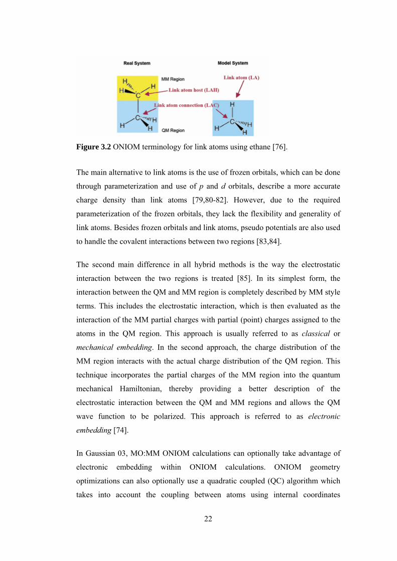
Figure 3.2 ONIOM terminology for link atoms using ethane [76].

The main alternative to link atoms is the use of frozen orbitals, which can be done

through parameterization and use of p and d orbitals, describe a more accurate

charge density than link atoms [79,80-82]. However, due to the required

parameterization of the frozen orbitals, they lack the flexibility and generality of

link atoms. Besides frozen orbitals and link atoms, pseudo potentials are also used

to handle the covalent interactions between two regions [83,84].

The second main difference in all hybrid methods is the way the electrostatic

interaction between the two regions is treated [85]. In its simplest form, the

interaction between the QM and MM region is completely described by MM style

terms. This includes the electrostatic interaction, which is then evaluated as the

interaction of the MM partial charges with partial (point) charges assigned to the

atoms in the QM region. This approach is usually referred to as classical or

mechanical embedding. In the second approach, the charge distribution of the

MM region interacts with the actual charge distribution of the QM region. This

technique incorporates the partial charges of the MM region into the quantum

mechanical Hamiltonian, thereby providing a better description of the

electrostatic interaction between the QM and MM regions and allows the QM

wave function to be polarized. This approach is referred to as electronic

embedding [74].

In Gaussian 03, MO:MM ONIOM calculations can optionally take advantage of

electronic embedding within ONIOM calculations. ONIOM geometry

optimizations can also optionally use a quadratic coupled (QC) algorithm which

takes into account the coupling between atoms using internal coordinates

23

(typically, those in the Small Model system) and those in Cartesian coordinates

(typically, the atoms only in the MM layer) in order to produce more accurate

steps. Note that optimizations in ONIOM proceed using the normal algorithms

and procedures. ONIOM affects only the energy and gradient computations

(ONIOM optimizations do not consist of independent, per-layer optimizations).

The use of an integrated potential surface also enables vibrational analysis to be

performed and related properties to be predicted [76].

3.3 Surface Models and Computational Methods

In this thesis work, water adsorption mechanisms on rutile (110), and water and

ammonia adsorption mechanisms on anatase (001) surfaces of TiO2 are

investigated by using ONIOM cluster method. In addition, water and ammonia

adsorption mechanisms on anatase TiO2 (001) slab surface are investigated by

means of periodic DFT method and the results are compared with the ones of

ONIOM cluster method.

ONIOM cluster calculations are performed by application of Gaussian 03 [87]

software, whereas periodic DFT calculations are carried out using VASP [95]

(Vienna ab-initio simulation package) code.

24

3.3.1 ONIOM Cluster Method

3.3.1.1 Surface Models

The first step applied to obtain ONIOM surface models is forming the crystalline

structures of bulk TiO2 (rutile and anatase). To do this the experimental

parameters of the bulk material; its space group, lattice parameters, atom

positions and unit cell formula, should be known. In Table 3.1 the experimental

parameters of bulk rutile TiO2 which are obtained from Wyckoff, 1963 [86] are

tabulated.

Table 3.1 Experimental parameters of TiO2 (Rutile). Space Group P42/mnm International Table No 136 Lattice Parameters a = b = 4.59373 A c = 2.95812 A u = 0.3053 AAtom Positions Ti : (2a) 000; 1/2 1/2 1/2 O : (4f) ± (uu0; u+1/2,1/2-u,1/2)

Data from [86].

The atomic parameters (X, Y, Z), called fractional coordinates, are determined by

applying atom positions to each atom considering their Wyckoff positions (2a) or

(4f). Table 3.2 illustrates the fractional coordinates of TiO2 (rutile) that are

evaluated by using atom positions given in Table 3.1.

Table 3.2 Atomic parameters (Fractional coordinates) of TiO2 (Rutile). Atom Position X Y Z

Ti (2a) 0.00000000 0.00000000 0.00000000 Ti (2a) 0.50000000 0.50000000 0.50000000 O (4f) 0.30530000 0.30530000 0.00000000 O (4f) 0.80530000 0.19470000 0.50000000 O (4f) -0.30530000 -0.30530000 0.00000000 O (4f) -0.80530000 -0.19470000 -0.50000000

25

The fractional coordinates are then multiplied by the respective lattice parameters

to find the Cartesian coordinates. Table 3.3 shows the Cartesian coordinates of

TiO2 (rutile) which are obtained by multiplying fractional coordinates shown in

Table 3.2 with the respective lattice parameters given in Table 3.1.

Table 3.3 Atomic parameters (Cartesian coordinates) of TiO2 (Rutile). Atom Position X Y Z

Ti (2a) 0.00000000 0.00000000 0.00000000 Ti (2a) 2.29686500 2.29686500 1.47906000 O (4f) 1.40246577 1.40246577 0.00000000 O (4f) 3.69933077 0.89439923 1.47906000 O (4f) -1.40246577 -1.40246577 0.00000000 O (4f) -3.69933077 -0.89439923 -1.47906000

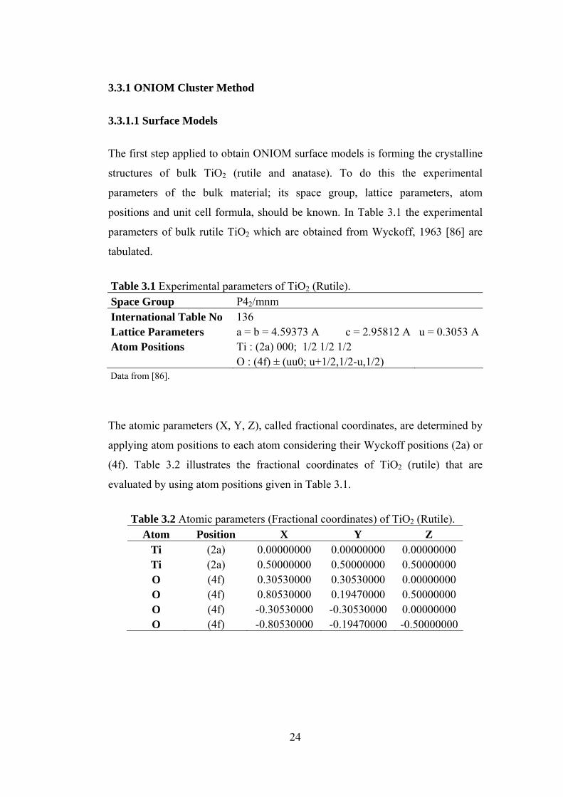
The Cartesian coordinates constitute the smallest repeated unit that is called unit

cell. TiO2 has a bimolecular unit cell so its unit cell formula is Ti2O4. The

structure of unit cell (Ti2O4) and the completed tetragonal cell (Ti9O6) are formed

in Gaussian 03 and presented in Figure 3.3 (a) and (b) respectively.

(a) (b)

Figure 3.3 (a) TiO2 (rutile) unit cell (Ti2O4). (b) The completed tetragonal cell (Ti9O6). Red balls are oxygen and gray ones are titanium atoms.

26

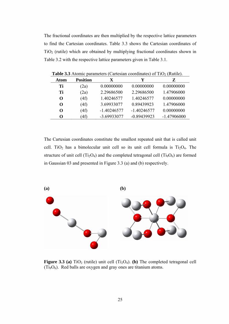
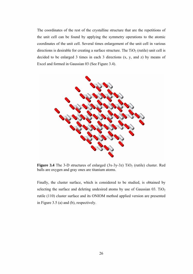
The coordinates of the rest of the crystalline structure that are the repetitions of

the unit cell can be found by applying the symmetry operations to the atomic

coordinates of the unit cell. Several times enlargement of the unit cell in various

directions is desirable for creating a surface structure. The TiO2 (rutile) unit cell is

decided to be enlarged 3 times in each 3 directions (x, y, and z) by means of

Excel and formed in Gaussian 03 (See Figure 3.4).

Figure 3.4 The 3-D structures of enlarged (3x-3y-3z) TiO2 (rutile) cluster. Red balls are oxygen and gray ones are titanium atoms.

Finally, the cluster surface, which is considered to be studied, is obtained by

selecting the surface and deleting undesired atoms by use of Gaussian 03. TiO2

rutile (110) cluster surface and its ONIOM method applied version are presented

in Figure 3.5 (a) and (b), respectively.

27

(a)

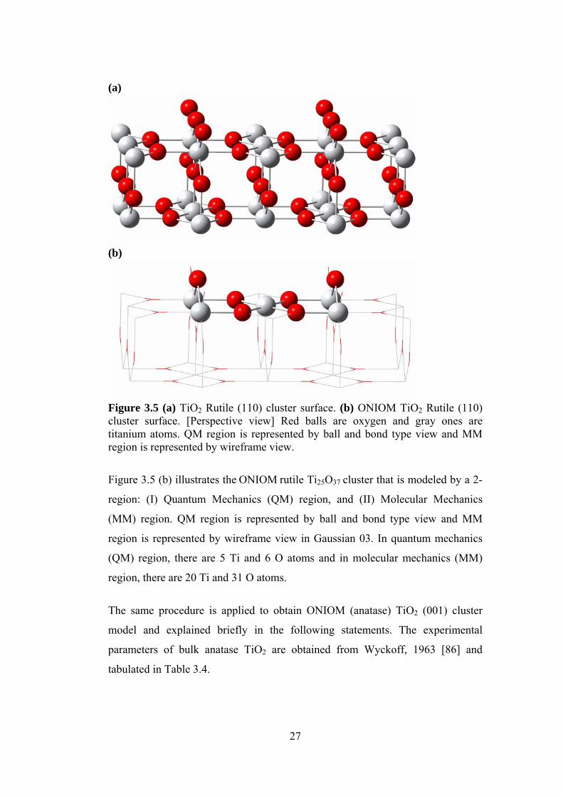
(b)

Figure 3.5 (a) TiO2 Rutile (110) cluster surface. (b) ONIOM TiO2 Rutile (110) cluster surface. [Perspective view] Red balls are oxygen and gray ones are titanium atoms. QM region is represented by ball and bond type view and MM region is represented by wireframe view.

Figure 3.5 (b) illustrates the ONIOM rutile Ti25O37 cluster that is modeled by a 2-

region: (I) Quantum Mechanics (QM) region, and (II) Molecular Mechanics

(MM) region. QM region is represented by ball and bond type view and MM

region is represented by wireframe view in Gaussian 03. In quantum mechanics

(QM) region, there are 5 Ti and 6 O atoms and in molecular mechanics (MM)

region, there are 20 Ti and 31 O atoms.

The same procedure is applied to obtain ONIOM (anatase) TiO2 (001) cluster

model and explained briefly in the following statements. The experimental

parameters of bulk anatase TiO2 are obtained from Wyckoff, 1963 [86] and

tabulated in Table 3.4.

28

Table 3.4 Experimental parameters of TiO2 (Anatase). Space Group I41/amd International Table No 141 Lattice Parameters a = b = 3.785 A c = 9.514 A u = 0.2066 AAtom Positions Ti : (4a) 000; 0 ½ ¼ B.C. O : (8e) 00u; 00-u; 0, ½, u+¼; 0, ½, ¼-u; B.C.

Data from [86].

Table 3.5 illustrates the fractional coordinates of TiO2 (anatase) which are

determined by means of atom positions given in Table 3.4.

Table 3.5 Atomic parameters (Fractional coordinates) of TiO2 (Anatase). Atom Position X Y Z

Ti (4a) 0.0000000 0.0000000 0.0000000 Ti (4a) 0.5000000 0.5000000 0.2500000 Ti (4a) 0.5000000 0.5000000 0.5000000 Ti (4a) 0.5000000 1.0000000 0.7500000 O (8e) 0.0000000 0.0000000 0.2066000 O (8e) 0.0000000 0.0000000 -0.2066000 O (8e) 0.0000000 0.5000000 0.4566000 O (8e) 0.0000000 0.5000000 0.0434000 O (8e) 0.5000000 0.5000000 0.7066000 O (8e) 0.5000000 0.5000000 0.2934000 O (8e) 0.5000000 1.0000000 0.9566000 O (8e) 0.5000000 1.0000000 0.5434000

Table 3.6 illustrates the Cartesian coordinates of TiO2 (anatase) which are

evaluated by multiplying fractional coordinates of TiO2 (anatase) shown in Table

3.5 with the respective lattice parameters given in Table 3.4.

29

Table 3.6 Atomic parameters (Cartesian coordinates) of TiO2 (Anatase). Atom Position X Y Z

Ti (4a) 0.000000 0.000000 0.000000 Ti (4a) 0.000000 1.892500 2.378500 Ti (4a) 1.892500 1.892500 4.757000 Ti (4a) 1.892500 3.785000 7.135500 O (8e) 0.000000 0.000000 1.965592 O (8e) 0.000000 0.000000 -1.965592 O (8e) 0.000000 1.892500 4.344092 O (8e) 0.000000 1.892500 0.412908 O (8e) 1.892500 1.892500 6.722592 O (8e) 1.892500 1.892500 2.791408 O (8e) 1.892500 3.785000 9.101092 O (8e) 1.892500 3.785000 5.169908

The structure of unit cell (Ti2O4) and the completed tetragonal cell (Ti11O18) are

formed in Gaussian 03 and presented in Figure 3.6 (a) and (b) respectively.

(a) (b)

Figure 3.6 (a) TiO2 (anatase) unit cell (Ti2O4). (b) The completed tetragonal cell (Ti11O18). Red balls are oxygen and gray ones are titanium atoms.

30

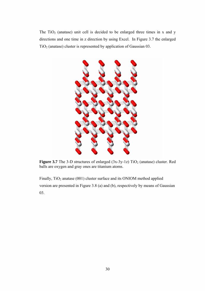
The TiO2 (anatase) unit cell is decided to be enlarged three times in x and y

directions and one time in z direction by using Excel. In Figure 3.7 the enlarged

TiO2 (anatase) cluster is represented by application of Gaussian 03.

Figure 3.7 The 3-D structures of enlarged (3x-3y-1z) TiO2 (anatase) cluster. Red balls are oxygen and gray ones are titanium atoms.

Finally, TiO2 anatase (001) cluster surface and its ONIOM method applied

version are presented in Figure 3.8 (a) and (b), respectively by means of Gaussian

03.

31

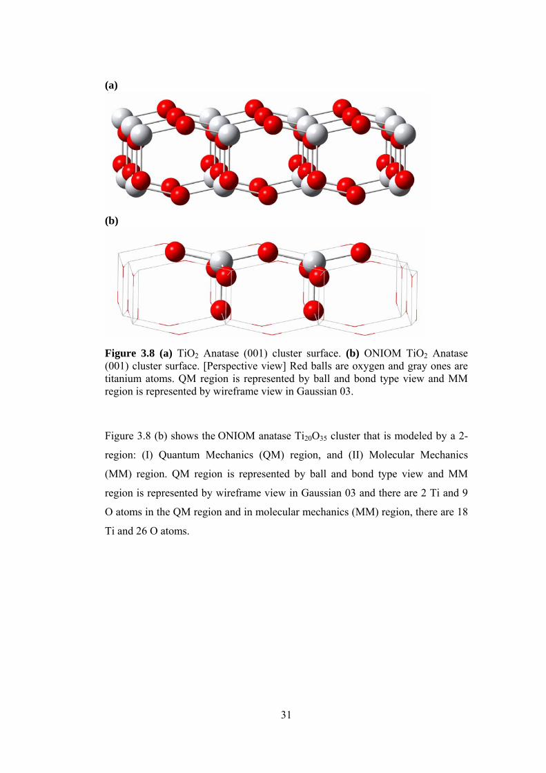
(a)

(b)

Figure 3.8 (a) TiO2 Anatase (001) cluster surface. (b) ONIOM TiO2 Anatase (001) cluster surface. [Perspective view] Red balls are oxygen and gray ones are titanium atoms. QM region is represented by ball and bond type view and MM region is represented by wireframe view in Gaussian 03.

Figure 3.8 (b) shows the ONIOM anatase Ti20O35 cluster that is modeled by a 2-

region: (I) Quantum Mechanics (QM) region, and (II) Molecular Mechanics

(MM) region. QM region is represented by ball and bond type view and MM

region is represented by wireframe view in Gaussian 03 and there are 2 Ti and 9

O atoms in the QM region and in molecular mechanics (MM) region, there are 18

Ti and 26 O atoms.

32

3.3.1.2. Computational Method

Quantum chemical calculations employing ONIOM DFT/B3LYP/6-31G**-

MM/UFF method provided in Gaussian 03 [87] are conducted to investigate the

energetics of water adsorption on rutile TiO2 (110), and water and ammonia

adsorption on anatase (001) cluster surfaces of TiO2.

In both ONIOM rutile and anatase cluster models, for quantum mechanical (QM)

region density functional theory (DFT) [88] calculations are conducted using

Becke’s [89,90] three-parameter hybrid method involving the Lee et al. [91]

correlation functional (B3LYP) formalism. The basis set employed in the DFT

calculations is 6-31G** for all atoms. For molecular mechanics (MM) region,

universal force field (UFF) [92] is used. Computations are carried out for partially

relaxed cluster representation where some of the atoms on QM region are relaxed

and the rest of the atoms are fixed.

The computational strategy used in this study is as follows: Initially, both the

cluster and the adsorbing molecule are optimized geometrically by means of

equilibrium geometry (optimized geometry or minimum-energy geometry)

calculations. Then, a coordinate driving calculation is initiated by selecting a

reaction coordinate distance between the adsorbing molecule and active site of the

cluster. Thus, the variation of the relative energy with decreasing distance is

obtained. Single point energy calculations are also performed where necessary by

locating the adsorbing molecule near the catalytic cluster. Provided unrestricted

calculations are performed, the <S2> value, spin contamination, is printed out and

compared with the value of s(s + 1) to check whether the spin contamination error

is negligible [72]. The relative energy is defined as:

ΔE = Esystem – (Ecluster + Eadsorbate)

where Esystem is the calculated energy of the given geometry containing the cluster

and the adsorbing molecule at any interatomic distance, Ecluster is the energy of the

cluster itself and Eadsorbate is that of the adsorbing molecule. Once having obtained

the energy profile, the geometry with the minimum energy on the energy profile

33

is re-optimized by means of the EG (equilibrium geometry) calculations to obtain

the final geometry for the reaction. For the calculated final geometry, vibration

frequencies are computed by the single point energy calculations. In this re-

optimization calculation, the reaction coordinate is not fixed. Finally, the

geometry with the highest energy from the energy profile is taken as the input

geometry for the transition state geometry calculations, and starting from these

geometries, the transition state structures with only one negative eigenvalue in

Hessian matrix are obtained. The synchronous quasi-Newtonian method of

optimization, (QST3) [93] is applied for transition state calculations.

Thermodynamic function values (ΔH˚, ΔG˚, and ΔS˚), for anatase phase only*, are

also calculated at specific temperatures which correspond to approximately the

experimental temperatures. The relevant equations are as follows:

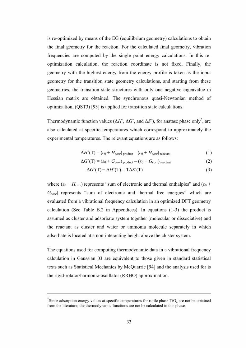
ΔH˚(T) = (ε0 + Hcorr) product – (ε0 + Hcorr) reactant (1)

ΔG˚(T) = (ε0 + Gcorr) product – (ε0 + Gcorr) reactant (2)

ΔG˚(T) = ΔH˚(T) – TΔS˚(T) (3)

where (ε0 + Hcorr) represents “sum of electronic and thermal enthalpies” and (ε0 +

Gcorr) represents “sum of electronic and thermal free energies” which are

evaluated from a vibrational frequency calculation in an optimized DFT geometry

calculation (See Table B.2 in Appendices). In equations (1-3) the product is

assumed as cluster and adsorbate system together (molecular or dissociative) and

the reactant as cluster and water or ammonia molecule separately in which

adsorbate is located at a non-interacting height above the cluster system.

The equations used for computing thermodynamic data in a vibrational frequency

calculation in Gaussian 03 are equivalent to those given in standard statistical

texts such as Statistical Mechanics by McQuarrie [94] and the analysis used for is

the rigid-rotator/harmonic-oscillator (RRHO) approximation.

*Since adsorption energy values at specific temperatures for rutile phase TiO2 are not be obtained from the literature, the thermodynamic functions are not be calculated in this phase.

34

3.3.2. Periodic DFT Method

3.3.2.1 Surface Model and Computational Method

The periodic DFT calculations are carried out by means of VASP [95] code,

which uses periodic plane wave basis sets. The electronic interactions are

described with PAW (projector augmented-wave) [96,97], and GGA (generalized

gradient approximation) [98] and the exchange and the correlation energy

proposed by Perdew and Wang (PW91) [99]. Except for the molecules and atoms

in the gas phase, dipole corrections are included for the asymmetric slab

calculations, where the top sides of the slabs are used. The cut-off energies and k-

points (Monkhorst Pack) used are; 500 eV and (3x3x1) for 4 layer p(2x2) anatase

TiO2 (001) slab (Figure 3.9). All the results reported in this work are carried out

by optimizing the respective structures until the net force acting on the atoms are

smaller than 0.01 eV/Å. The atoms and the molecules in the gas phase are

represented with the same level of precision by surrounding the species with a

vacuum layer of minimum 10 Å in all directions.

Figure 3.9 Four layer p(2x2) TiO2 anatase (001) slab.

Anatase TiO2 (001) surface slab (Figure 3.9) is prepared by initially optimizing

the respective crystal and then cutting the crystal along (001) plane and placing a

15 Å vacuum layer above.

35

The adsorption energy is calculated for adsorbate on the clean surface as follows:

Eadsorption = Eadsorbate/surface– (Eadsorbate + Esurface)

where Eadsorbate is the energy of the isolated molecule (H2O or NH3) in the

vacuum. Esurface is the energy of a clean anatase (001) surface, and Eadsorbate/surface is

the total energy of the molecule adsorbed together with the (001) anatase TiO2

surface. One side of the slab is occupied by adsorbed molecules. The coverage of

adsorbed molecules is taken as θ=0.25 with respect to surface Ti atoms.

The vibrational frequencies of adsorbed surface species are also calculated, after

the optimizations to equilibrium geometries as described above. This is done by

using the "IBRION = 5" parameter that turns on the calculation of the exact

Hessian matrix. The Hessian matrix is calculated based on a finite difference

approach with a step size of 0.02 for the displacements of the individual atoms of

the adsorbate along each direction. The frequencies are calculated for the

optimized geometries of minimas, by turning off the symmetry parameters. The

frequencies of the unfrozen surface atoms (phonons) are also calculated, however

they are not reported herein.

36

CHAPTER 4

RESULTS AND DISCUSSION

4.1 ONIOM Cluster Method

4.1.1 Water Adsorption on Rutile TiO2 (110) Cluster Surface

4.1.1.1 Optimization of Cluster

Optimization (equilibrium geometry calculations) of ONIOM rutile TiO2 (110)

cluster is conducted by using DFT method, B3LYP formalism, 6-31G** basis set

for QM region, and UFF for MM region. Computations are carried out taking the

total charge as neutral, the spin multiplicity as 6, and for partially relaxed cluster

representation where some of the atoms on QM region, (Ti1, O1 and O2), are

relaxed and the rest of the atoms are fixed. Optimized geometry of 2-region

ONIOM Ti25O37 cluster is shown in Figure 4.1.

Figure 4.1 Optimized geometry of 2-region ONIOM rutile TiO2 (110) cluster model. QM region is represented by ball and bond type view and MM region is represented by wireframe view.

37

The comparison of atomic displacements away from the rutile TiO2 (110) surface

relative to an ideal bulk structure with the available literature data is illustrated in

Table 4.1. The variation in the distance of Ti1 from the surface in z-direction (∆z)

is calculated to be -0.14 Å. The corresponding results in the experimental

literatures are -0.19 ± 0.03 Å [100], -0.16 ± 0.05 Å [101] and in the theoretical

literatures is - 0.17 Å [102]. The variation (Δz) in the distance of O2 from the

surface is calculated to be -0.14 Å. The corresponding results in the experimental

and theoretical literatures are 0.10 ± 0.05 Å [100] and -0.27 ± 0.08 Å [101] and -

0.01 Å [102], respectively. Table 4.1 points out that the results obtained in this

study agree very well with the literature values (See Figure 4.1 for Ti1 and O2).

Table 4.1 The comparison of the atomic displacements away from the rutile TiO2 (110) surface relative to an ideal bulk structure with the available literature values.

Experimental Other Theoretical Atom This study d

LEED-IVa SXRDb HFc DFT-LDAc

Ti1 ∆z (Å) -0.14 -0.19 ± 0.03 -0.16 ± 0.05 -0.17 -0.17 O2 ∆z (Å) 0.05 0.10 ± 0.05 -0.27 ± 0.08 -0.01 -0.01

a Lindsay et al. [100] b Charlton et al. [101] c Swamy et al. [102] d Erdogan et al. [112]

38

4.1.1.2 Molecular Adsorption Mechanism

For molecular water adsorption on rutile TiO2 (110) surface, a reaction coordinate

is selected as the distance between the O atom (O3) of the water molecule and the

fivefold coordinated Ti atom (Ti1) in QM region. As seen from the equilibrium

geometry and energy profile (see Figure 4.2), molecular water adsorption occurs

on partially relaxed ONIOM cluster with an exothermic relative energy difference

of 22.4 kcal/mol and with (Ti1-O3) distance of 2.32 Å, and (H2-O2) distance of

1.95 Å.

Figure 4.2 Relative energy profile and equilibrium geometry of molecular H2O adsorption on rutile TiO2 (110) surface. QM region is represented by ball and bond type view and MM region is represented by wireframe view.

39

4.1.1.3 Dissociative Adsorption Mechanism

Dissociative water adsorption is achieved on rutile TiO2 (110) surface starting

from the optimized geometry of molecular water adsorption. For this purpose, a

reaction coordinate is selected as the distance between the hydrogen atom (H2) of

the water molecule and the bridging oxygen atom (O2) of the cluster. (See Figure

4.4 for H2 and O2). As can be observed from the energy profile obtained for this

reaction, illustrated in Figure 4.3, water dissociatively adsorbs on the surface with

an activation barrier value of 23.2 kcal/mol.

Figure 4.3 Relative energy profile for dissociative H2O adsorption on rutile TiO2 (110) surface.

Figure 4.4 (a) shows equilibrium geometry of dissociative water adsorption on

rutile TiO2 (110) surface. H2O is dissociatively adsorbed on the surface with (Ti1-

O3) distance of 1.84 Å, (H2-O3) distance of 2.41 Å, and (H2-O2) distance of 0.98

Å. Transition state geometry of this interaction is also illustrated in Figure 4.4 (b).

One imaginary frequency is found as -776 cm-1 at transition state mode. The

corresponding distances (Ti1-O3), (H2-O3), (H2-O2) for the transition state

geometry are 2.23 Å, 1.44 Å, and 1.07 Å, respectively.

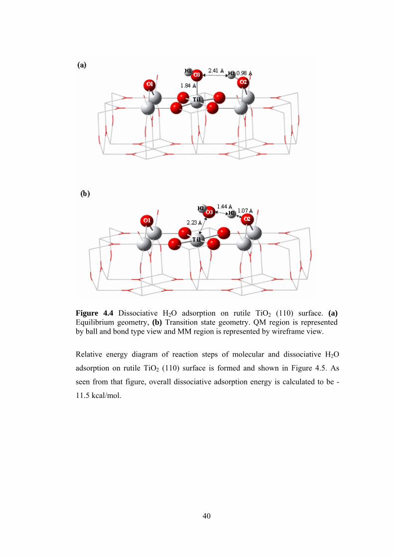
40

Figure 4.4 Dissociative H2O adsorption on rutile TiO2 (110) surface. (a) Equilibrium geometry, (b) Transition state geometry. QM region is represented by ball and bond type view and MM region is represented by wireframe view.

Relative energy diagram of reaction steps of molecular and dissociative H2O

adsorption on rutile TiO2 (110) surface is formed and shown in Figure 4.5. As

seen from that figure, overall dissociative adsorption energy is calculated to be -

11.5 kcal/mol.

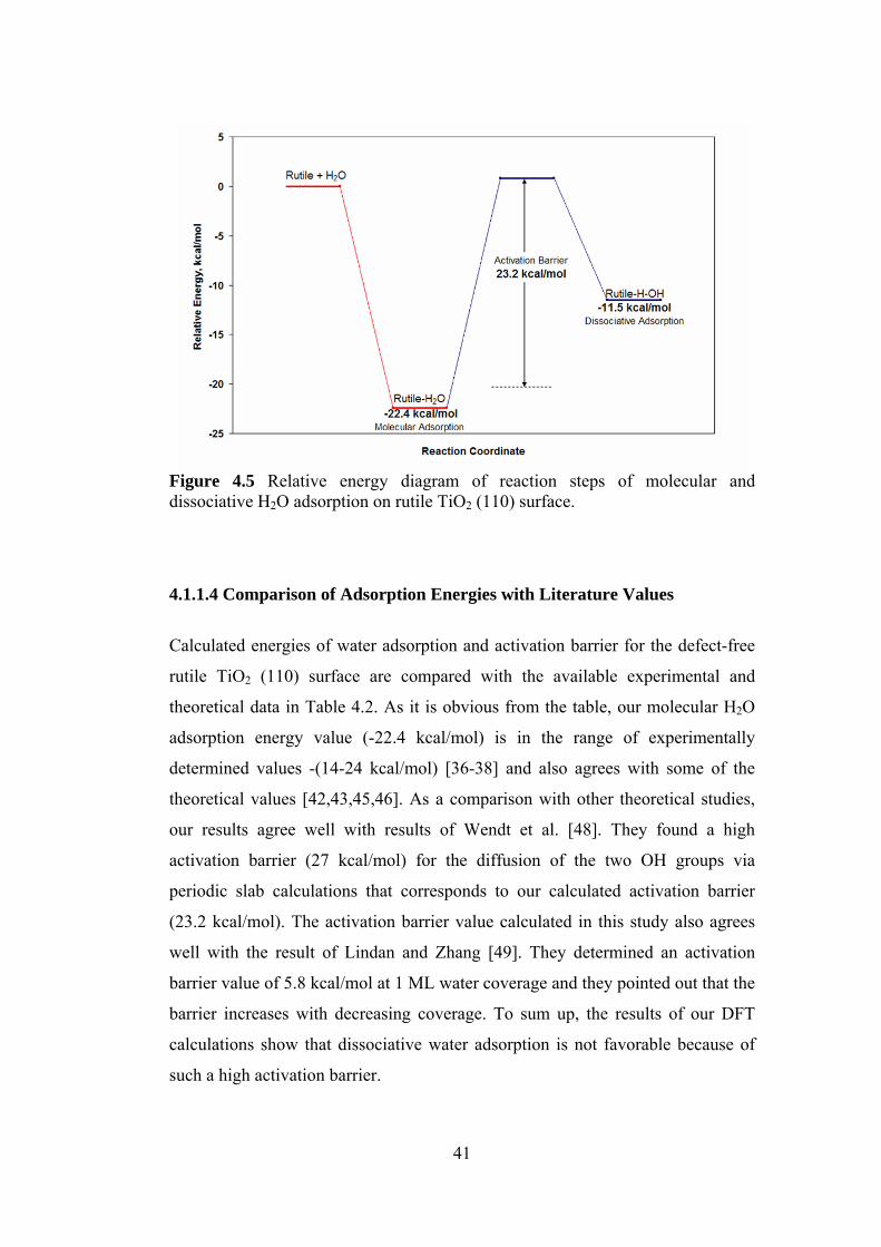
41

Figure 4.5 Relative energy diagram of reaction steps of molecular and dissociative H2O adsorption on rutile TiO2 (110) surface.

4.1.1.4 Comparison of Adsorption Energies with Literature Values

Calculated energies of water adsorption and activation barrier for the defect-free

rutile TiO2 (110) surface are compared with the available experimental and

theoretical data in Table 4.2. As it is obvious from the table, our molecular H2O

adsorption energy value (-22.4 kcal/mol) is in the range of experimentally

determined values -(14-24 kcal/mol) [36-38] and also agrees with some of the

theoretical values [42,43,45,46]. As a comparison with other theoretical studies,

our results agree well with results of Wendt et al. [48]. They found a high

activation barrier (27 kcal/mol) for the diffusion of the two OH groups via

periodic slab calculations that corresponds to our calculated activation barrier

(23.2 kcal/mol). The activation barrier value calculated in this study also agrees

well with the result of Lindan and Zhang [49]. They determined an activation

barrier value of 5.8 kcal/mol at 1 ML water coverage and they pointed out that the

barrier increases with decreasing coverage. To sum up, the results of our DFT

calculations show that dissociative water adsorption is not favorable because of

such a high activation barrier.

42

Table 4.2 The comparison of the calculated energies of H2O adsorption and activation barrier on rutile TiO2 (110) surface with the theoretical and experimental values in the literature. Energy, kcal/mol

References Molec. Ads.

Disso. Ads.

Act. Barr. Method and Software

Theoretical Lindan et al. 1998 [42] -22.9 -21.0 - DFT-GGA-PW91 1 ML

CASTEP Casarin et al. 1998 [43] -19.3 - - DFT-LDA-GGA-BP ADF Stefanovich et al. 1999 [44] -34.5 -7.9 - LCAO:HF LANL1-CEP -34.9 -22.6 - LCAO:B3LYP LANL1-CEP -34.4 -18.0 - LCAO:MP2 Gaussian 92 Menetrey et al. 2003 [45] -22.1 -29.3 - DFT-GGA-PW91 9L 1/3ML

VASP Bandura et al. 2004 [46] -22.5 -11.5 - LCAO:HF LANL1-CEP

Gaussian 98 -21.9 -18.4 - PW:DFT-GGA-PW91 5L

CASTEP Wendt et al. 2005 [47] -15.2 -18.2 - PW:DFT-GGA-RPBE

DACAPO Wendt et al. 2006 [48] - - 27.0 PW:DFT-GGA-RPBE Lindan and Zhang 2005 [49] -11.8 -6.5 5.8 DFT-GGA-PW91 5L 1ML

CASTEP Kamisaka et al. 2007 [51] -18.4 -13.4 - DFT-GGA-PW91 1/3 ML -16.1 -10.6 - DFT-GGA-PBE 1/3 ML

VASP Erdogan et al. 2009 [112] -22.4 -11.5 23.2 ONIOM

DFT/B3LYP/6-31G** -MD/UFF Gaussian 03

Experimental Hugenshimidt et al.1994 [36] -(17-21.5) XPS, TPD, work function Henderson et al. 1996 [37] -(17-19) TPD Brinkley et al. 1998 [38] -(14-24) TPD, Modulated Beams

There are also controversial results in theoretical literature regarding water

adsorption on perfect rutile TiO2 (110) surface as can be seen in Table 4.2. The

variations in the results of theoretical literature may be explained by the usage of

different quantum chemical methods, cluster models, basis sets, coverages, etc.

The result obtained in this study for molecular adsorption energy value (-22.4

kcal/mol) agrees well with the result (-19.3 kcal/mol) reported by Casarin et al.

[43]. However, they did not study or could not find a dissociation case. Results in

the study of Lindan and Zhang [49] are different from this study and it may be

due to the coverage effect as they studied adsorption at high water coverage (1

43

monolayer), whereas we used low water coverage. The most probable reasons for

the difference from the results of Stefanovich et al. [44] may be that they used

different quantum chemical methods, functionals and basis sets and a very old

version software program (Gaussian 92). Unlike most of other theoretical results,

Menetrey et al. [45] predicted that dissociative adsorption on rutile TiO2 (110)

surface is more favorable than molecular one and the reason for the disagreement

is unclear. It may not be related with coverage effect since when they decrease the

coverage; the trend (dissociative adsorption’s being favorable) is maintained.

However, recent VASP study published by Kamisaka et al. [51] and cluster study

reported by Bandura et al. [46] support our results for molecular and dissociative

water adsorption energies. Results obtained in this study for molecular and

dissociative water adsorption energy values (-22.4 kcal/mol and -11.5 kcal/mol,

respectively) are quite similar to what Kamisaka et al. [51] determined (-18.4

kcal/mol vs. -13.4 kcal/mol, respectively) using VASP and exactly same to what

Bandura et al. [46] obtained (-22.5 kcal/mol vs. -11.5 kcal/mol, respectively)

using Gaussian 98.

4.1.1.5 Vibrational Frequency Studies

Table 4.3 presents the structural and vibrational properties of molecularly, and

dissociatively adsorbed H2O molecule on rutile TiO2 (110) surface with relevant

experimental data. Asymmetric OH, symmetric OH, and bending HOH vibration

data of 3705, 3489, 1566 cm-1 for molecular water adsorption are in agreement

with the experimental [37] values of 3625, 3420, 1625 cm-1, respectively. The

frequency of terminal hydroxyl for dissociative water adsorption is computed in

this study as 3668 cm-1 that is in agreement with the experimental value of 3690

cm-1 reported by Henderson et al. [37]. They also reported that the small amount

of water dissociation observed by HREELS on ideal TiO2 (110) surface under

UHV conditions; but that dissociation may be linked to structural and/or point

defects. Frequency of deposited proton is computed as 3536 cm-1 and relevant

experimental data is not available in the literature.

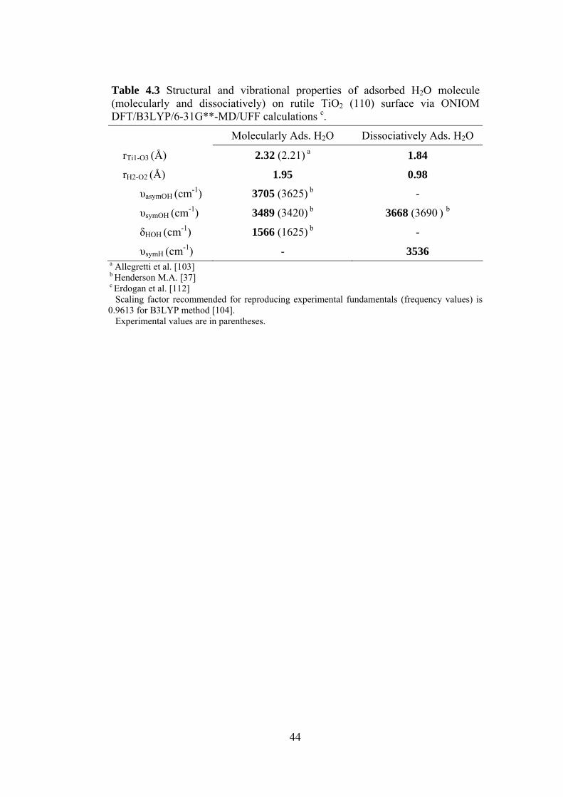
44

Table 4.3 Structural and vibrational properties of adsorbed H2O molecule (molecularly and dissociatively) on rutile TiO2 (110) surface via ONIOM DFT/B3LYP/6-31G**-MD/UFF calculations c.

Molecularly Ads. H2O Dissociatively Ads. H2O

rTi1-O3 (Å) 2.32 (2.21) a 1.84

rH2-O2 (Å) 1.95 0.98

υasymOH (cm-1) 3705 (3625) b -

υsymOH (cm-1) 3489 (3420) b 3668 (3690 ) b

δHOH (cm-1) 1566 (1625) b -

υsymH (cm-1) - 3536 a Allegretti et al. [103] b Henderson M.A. [37] c Erdogan et al. [112] Scaling factor recommended for reproducing experimental fundamentals (frequency values) is 0.9613 for B3LYP method [104]. Experimental values are in parentheses.

45

4.1.2 Water and Ammonia Adsorption on Anatase TiO2 (001) Cluster Surface

4.1.2.1 Optimization of Cluster

Optimization of ONIOM anatase TiO2 (001) cluster is conducted by using DFT

method, B3LYP formalism, 6-31G** basis set for QM region, and UFF for MM

region. Computations are carried out by taking the total charge as neutral, the spin

multiplicity as 2, and for partially relaxed cluster representation where some of

the atoms on QM region, (Ti1, O1 and Ti2), are relaxed and the rest of the atoms

are fixed. Optimized geometry of 2-region ONIOM Ti20O35 cluster model is

shown in Figure 4.6.

Figure 4.6 Optimized geometry of 2-region ONIOM anatase TiO2 (001) cluster model. QM region is represented by ball and bond type view and MM region is represented by wireframe view.

Fivefold coordinated titanium atoms (Ti1 and Ti2) (act as Lewis acid sites) and

the surface oxygen atoms (O1) (have Bronsted base properties) were reported as

the catalytic active sites of TiO2 anatase in [55,57] and illustrated in Figure 4.6.

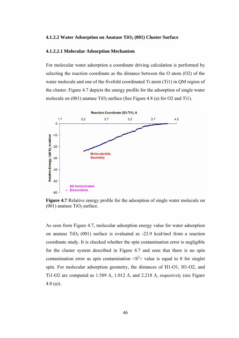
46

4.1.2.2 Water Adsorption on Anatase TiO2 (001) Cluster Surface

4.1.2.2.1 Molecular Adsorption Mechanism

For molecular water adsorption a coordinate driving calculation is performed by

selecting the reaction coordinate as the distance between the O atom (O2) of the

water molecule and one of the fivefold coordinated Ti atom (Ti1) in QM region of

the cluster. Figure 4.7 depicts the energy profile for the adsorption of single water

molecule on (001) anatase TiO2 surface (See Figure 4.8 (a) for O2 and Ti1).

Figure 4.7 Relative energy profile for the adsorption of single water molecule on (001) anatase TiO2 surface.

As seen from Figure 4.7, molecular adsorption energy value for water adsorption

on anatase TiO2 (001) surface is evaluated as -23.9 kcal/mol from a reaction

coordinate study. It is checked whether the spin contamination error is negligible

for the cluster system described in Figure 4.7 and seen that there is no spin

contamination error as spin contamination <S2> value is equal to 0 for singlet

spin. For molecular adsorption geometry, the distances of H1-O1, H1-O2, and

Ti1-O2 are computed as 1.589 Å, 1.012 Å, and 2.218 Å, respectively (see Figure

4.8 (a)).

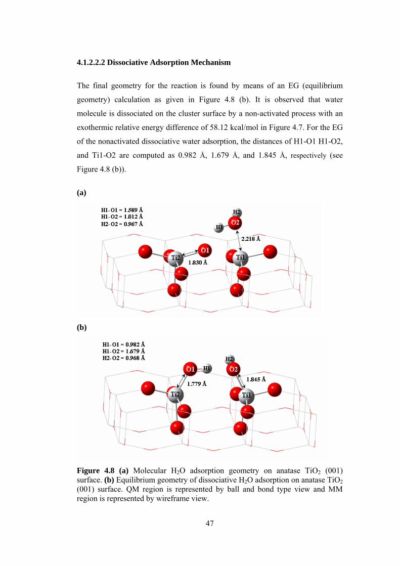
47

4.1.2.2.2 Dissociative Adsorption Mechanism

The final geometry for the reaction is found by means of an EG (equilibrium

geometry) calculation as given in Figure 4.8 (b). It is observed that water

molecule is dissociated on the cluster surface by a non-activated process with an

exothermic relative energy difference of 58.12 kcal/mol in Figure 4.7. For the EG

of the nonactivated dissociative water adsorption, the distances of H1-O1 H1-O2,

and Ti1-O2 are computed as 0.982 Å, 1.679 Å, and 1.845 Å, respectively (see

Figure 4.8 (b)).

(a)

(b)

Figure 4.8 (a) Molecular H2O adsorption geometry on anatase TiO2 (001) surface. (b) Equilibrium geometry of dissociative H2O adsorption on anatase TiO2 (001) surface. QM region is represented by ball and bond type view and MM region is represented by wireframe view.

48

4.1.2.2.3 Comparison of Adsorption Energies with Literature Values

The computed molecular and dissociative adsorption energy values for water on

anatase TiO2 surface (001) are given in Table 4.4 with the available theoretical

and experimental literature data for comparison. Experimental studies by Srnak et

al. [52] and Munuera et al. [53] have reported molecular adsorption of water on

TiO2 (anatase) surface only. As also observed from Table 4.4, in our study and

other published studies [13,60-62,64-66,68-70], water molecule is dissociated by

a non-activated process or the computed adsorption energy value for dissociative

adsorption is lower than the molecular one. Thus, dissociative adsorption of water

molecule is energetically favored on anatase TiO2 (001) surface.

Table 4.4 A comparison of the calculated H2O adsorption energies (kcal/mol) on perfect anatase TiO2 (001) surface with the theoretical and experimental values in the literature.

Adsorption Energy Authors and References Method Molec. Dissoc.

Theoretical Fahmi and Minot 1994 [60] Periodic -14.34 -28.68 Bredow et al. 1995 [61] MO/SINDO1 4x4x3 cluster -25.33 -31.79 3x3x3 cluster -32.50 -38.72 2x2x3 cluster -35.61 -52.82 Vittadini et al. 1998 [13] PW:DFT-GGA Car-Parrinello -18.68 -33.21 Nair 2004 [64] DFT -18.64 -32.98 Arrouvel et al. 2004 [65] PW:DFT-GGA KS - -(24-39) Jug et al. 2005 [62] MSINDO -23.90 -49.71 Gong and Selloni 2005 [66] PW:DFT-GGA Car-Parrinello

1/6 ML- -28.80

1/3 ML - -25.60 1/2 ML - -26.98 Ignatchenko et al. 2006 [68] DN-PW91 1/2 ML - -45.30 DNP-PW91 1/2 ML - -41.00 DNP-PBE 1/2 ML - -39.90 DNP-PBE (1xn) H2O add. - -38.50 Wahab et al. 2008 [69] MSINDO -17.69 -24.62 Onal et al. 2006 [70] DFT-B3LYP/6-31G** Relax. -24.93 -54.00 Erdogan et al. 2009 [113] ONIOM DFT/B3LYP/

6-31G**-MD/UFF -23.90 -33.67

Experimental Srnak et al. 1992 [52] TPD Anatase TiO2 -11, -18 Munuera et al. 1999 [53] TPD Anatase TiO2 -12

49

4.1.2.2.4 Vibrational Frequency Studies

The vibration frequency values of dissociatively adsorbed H2O on (001) anatase

TiO2 surface are calculated by single point energy calculations. A comparison of

the results with the available experimental literature is given in Table 4.5. As seen

in the table, the O–H stretching vibration value of 3657 cm-1 computed for

dissociative water adsorption agrees well with the experimental values of (3665,

3715 cm-1) where (001) anatase surface was assumed [105] and it is also in the

experimentally predicted range (3600–3800 cm-1) reported by another reference

[106].

a Primet et al. [105] bMorterra et al. [106] c Erdogan et al. [113] Scaling factor recommended for reproducing experimental fundamentals (frequency values) is 0.9613 for B3LYP method [104].

4.1.2.2.5 Thermochemical Data at Specific Temperatures

Table 4.6 shows calculated reaction enthalpy, free energy (kcal/mol) and entropy

(cal/mol.K) values at 0 K and at specific experimental temperatures (170, 260 K)

[52] for molecular or dissociative H2O adsorption on anatase TiO2 (001) surface.

As can be seen from the table, there is no remarkable difference between the

calculated reaction enthalpies in this range of temperatures. Our results also

indicate that calculated reaction enthalpies for molecular water adsorption at 170

K and 260 K (-22.2 kcal/mol and -22 kcal/mol, respectively) are approximately

close to one of the experimentally obtained desorption enthalpies of adsorbed

states of water (-18 kcal/mol) [52]. It should be noted that these experimental

Table 4.5 Vibrational frequencies (cm-1) of dissociatively adsorbed H2O molecule on anatase TiO2 (001) surface as obtained from ONIOM DFT/B3LYP-6-31G**-MD/UFF calculations.

This work c

Anatase (001) TiO2 Experimental Anatase TiO2

υsymOH stret. 3657 3665a, 3715a, 3600-3800b

50

results are obtained for titania (anatase) material, which may include all types of

surfaces rather than the specific (001) surface.

Table 4.6 Calculated ΔH˚, ΔG˚ (kcal/mol), and ΔS˚ (cal/mol.K) values at 0 K and specific experimental temperatures (170, 260 K) [52] for H2O adsorption on anatase TiO2 (001) surface b.

Molecularly Adsorbed H2O

Dissociatively Adsorbed H2O

At 0 K ΔH˚ = ΔG˚ -23.9 -58.1 At 170 K ΔH˚ -22.2 (-18)a -51.9 ΔG˚ -21.7 -50.9 ΔS˚ -2.8 -6.2 At 260 K ΔH˚ -22.0 (-11)a -52.0 ΔG˚ -21.5 -50.3 ΔS˚ -2.2 -6.8

a Srnak et al. [52] b Erdogan et al. [113] Experimental values are in parentheses and belong to titania (anatase) material which may include many types of surfaces and not specifically (001) surface.

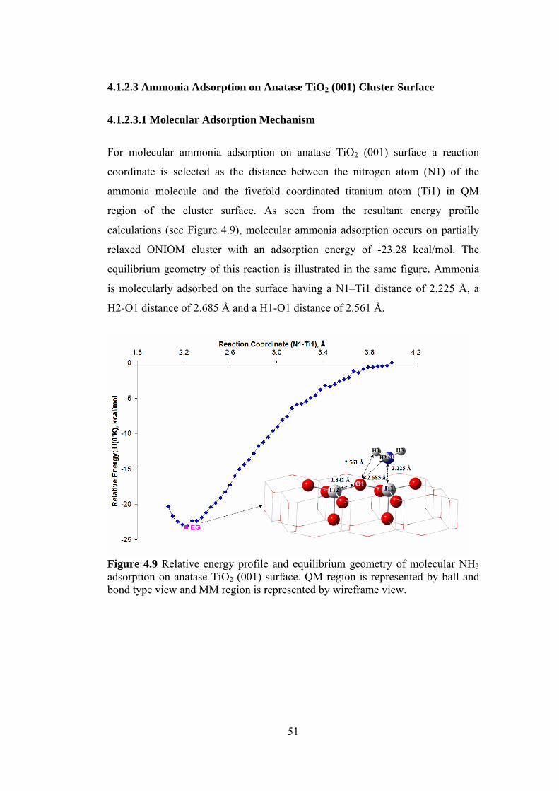
51

4.1.2.3 Ammonia Adsorption on Anatase TiO2 (001) Cluster Surface


For molecular ammonia adsorption on anatase TiO2 (001) surface a reaction

coordinate is selected as the distance between the nitrogen atom (N1) of the

ammonia molecule and the fivefold coordinated titanium atom (Ti1) in QM

region of the cluster surface. As seen from the resultant energy profile

calculations (see Figure 4.9), molecular ammonia adsorption occurs on partially

relaxed ONIOM cluster with an adsorption energy of -23.28 kcal/mol. The

equilibrium geometry of this reaction is illustrated in the same figure. Ammonia

is molecularly adsorbed on the surface having a N1–Ti1 distance of 2.225 Å, a

H2-O1 distance of 2.685 Å and a H1-O1 distance of 2.561 Å.

Figure 4.9 Relative energy profile and equilibrium geometry of molecular NH3 adsorption on anatase TiO2 (001) surface. QM region is represented by ball and bond type view and MM region is represented by wireframe view.

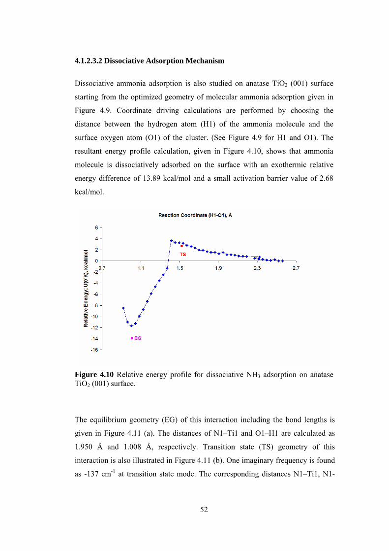
52


Dissociative ammonia adsorption is also studied on anatase TiO2 (001) surface

starting from the optimized geometry of molecular ammonia adsorption given in

Figure 4.9. Coordinate driving calculations are performed by choosing the

distance between the hydrogen atom (H1) of the ammonia molecule and the

surface oxygen atom (O1) of the cluster. (See Figure 4.9 for H1 and O1). The

resultant energy profile calculation, given in Figure 4.10, shows that ammonia

molecule is dissociatively adsorbed on the surface with an exothermic relative

energy difference of 13.89 kcal/mol and a small activation barrier value of 2.68

kcal/mol.

Figure 4.10 Relative energy profile for dissociative NH3 adsorption on anatase TiO2 (001) surface.

The equilibrium geometry (EG) of this interaction including the bond lengths is

given in Figure 4.11 (a). The distances of N1–Ti1 and O1–H1 are calculated as

1.950 Å and 1.008 Å, respectively. Transition state (TS) geometry of this

interaction is also illustrated in Figure 4.11 (b). One imaginary frequency is found

as -137 cm-1 at transition state mode. The corresponding distances N1–Ti1, N1-

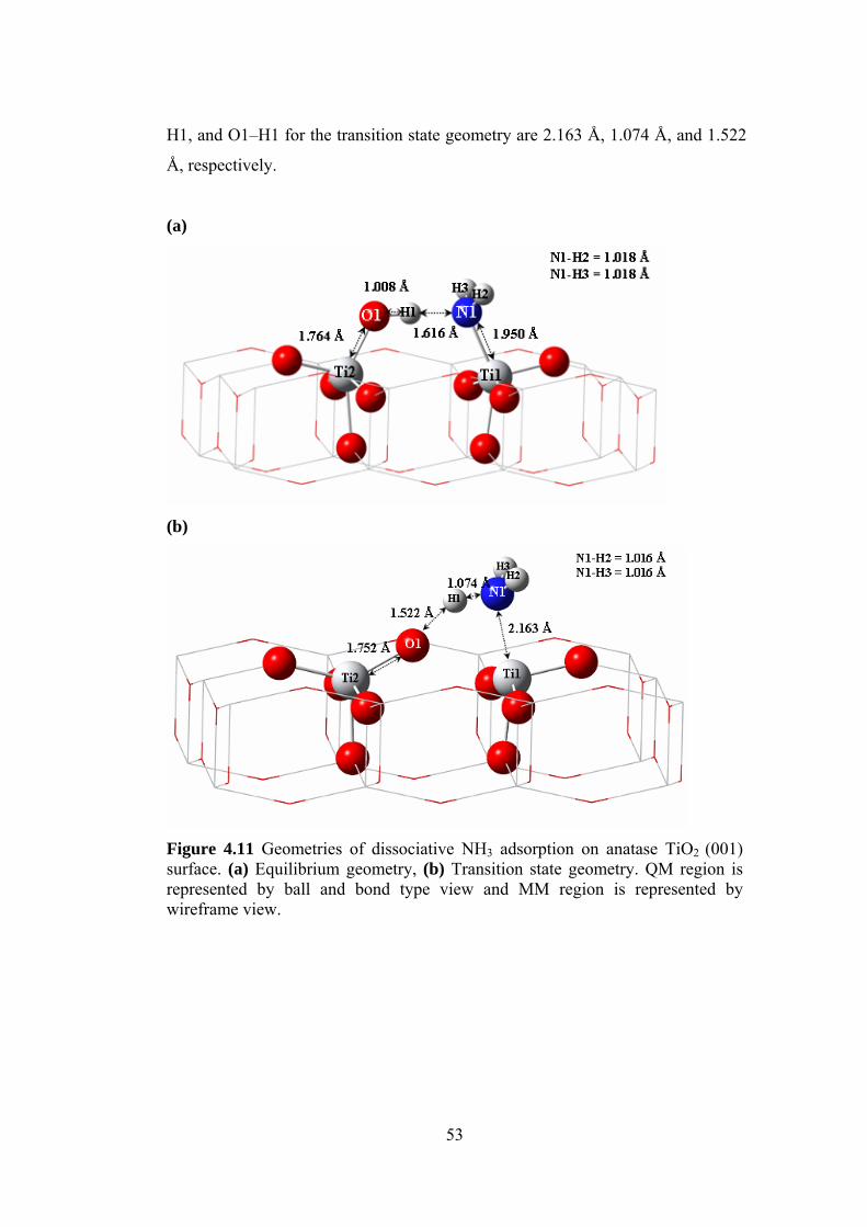
53

H1, and O1–H1 for the transition state geometry are 2.163 Å, 1.074 Å, and 1.522

Å, respectively.

(a)

(b)

Figure 4.11 Geometries of dissociative NH3 adsorption on anatase TiO2 (001) surface. (a) Equilibrium geometry, (b) Transition state geometry. QM region is represented by ball and bond type view and MM region is represented by wireframe view.

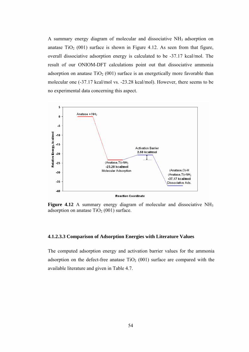
54

A summary energy diagram of molecular and dissociative NH3 adsorption on

anatase TiO2 (001) surface is shown in Figure 4.12. As seen from that figure,

overall dissociative adsorption energy is calculated to be -37.17 kcal/mol. The

result of our ONIOM-DFT calculations point out that dissociative ammonia

adsorption on anatase TiO2 (001) surface is an energetically more favorable than

molecular one (-37.17 kcal/mol vs. -23.28 kcal/mol). However, there seems to be

no experimental data concerning this aspect.

Figure 4.12 A summary energy diagram of molecular and dissociative NH3 adsorption on anatase TiO2 (001) surface.


The computed adsorption energy and activation barrier values for the ammonia

adsorption on the defect-free anatase TiO2 (001) surface are compared with the

available literature and given in Table 4.7.

55

Table 4.7 A comparison of the calculated NH3 adsorption energies on anatase TiO2 (001) surface with the theoretical and experimental values in the literature.

Adsorption Energy, kcal/mol Authors and References Method

Molec. Dissoc. Act. Barrier

Theoretical Onal et al. 2006 [70] DFT-B3LYP-6-31G** -26.57 -36.32 3.63 Calatayud et al 2004 [71] DFT -19.40 -

Erdogan et al. [113] ONIOM DFT/B3LYP/6-31G**-MD/UFF

-23.28 -37.17 2.68

Experimental (Anatase TiO2) Srnak et al. 1992 [52] TPD -14, -27 Sprinceana et al. 1999 [59] XRD BET -(31-36)

Experimental works involving TPD [52] and XRD, BET [59] studied NH3

adsorption on TiO2 (anatase) only. However, the computed molecular NH3

adsorption energy value of -23.28 kcal/mol is comparable with -27 kcal/mol of

NH3 desorption enthalpy value reported by Srnak et al. [52]. The slight deviation

is reasonable in view of the fact that (001) surface is minority in anatase as

previously mentioned. There seems to be only two theoretical studies concerning

NH3 adsorption on (001) anatase TiO2 [70,71]. Molecular and dissociative NH3

adsorption energy values (-23.28 kcal/mol and -37.17 kcal/mol, respectively)

obtained in this study are quite comparable to what Onal et al. [70] obtained (-

26.57 kcal/mol vs. -36.32 kcal/mol, respectively) using SPARTAN’04 software.

The activation barrier value (2.68 kcal/mol) calculated in this study also agrees

well with their activation barrier value of 3.63 kcal/mol. Calatayud et al. [71]

reported a molecular NH3 adsorption energy as -19.4 kcal/mol using periodic DFT

calculations. However, they did not study or could not find a dissociation case.

56


Vibration frequencies for ammonia adsorption on anatase TiO2 (001) cluster

surface are also calculated by single point energy calculations. Table 4.8 shows

the vibrational properties of molecularly and dissociatively adsorbed NH3

molecule on the (001) surface with available experimental data reported for

anatase surfaces in general.

Table 4.8 The vibrational frequency (cm-1) properties of molecularly and dissociatively adsorbed NH3 molecule on anatase TiO2 (001) surface as obtained from ONIOM DFT/B3LYP-MD/UFF calculations with the experimental literature values e. Molecularly Ads. NH3 Dissociatively Ads. NH3

EG EG TS

υasymHNH stret. 3485, 3494 (3400c) 3463 3482 υsymHNH stret. 3347 (3350c) 3365 3395 δasymHNH bend. 1576, 1586 (1599a, 1600c) - 1573 δsymHNH bend. 1086 (1190a, 1225a, 1215b) - 1082 υHNH scis. - 1464 (1480c, 1540d) 1514

a Amores et al. [107] b Teramura et al. [108] c Schneider et al. [109] d Lietti et al. [110] e Erdogan et al. [113] Scaling factor recommended for reproducing experimental fundamentals (frequency values) is 0.9613 for B3LYP method [104]. Experimental values are in parentheses and particular surface of the TiO2 (anatase) has not been reported. As it is seen from the Table 4.8, symmetric bending frequency value of 1086 cm−1

and asymmetric stretching frequency data of (3485 cm−1, 3494 cm−1) for

molecular ammonia adsorption deviate significantly from the experimental values

of 1190 cm−1, 1225 cm−1 [107] and 1215 cm−1 [108] and of 3400 cm−1 [109],

respectively. On the other hand, asymmetric bending (1576 cm−1, 1586 cm-1), and

symmetric stretching (3347 cm-1), vibration data for molecular ammonia

adsorption are in agreement with the experimental values of (1599 cm−1 [107],

1600 cm-1 [109]), and 3350 cm-1 [109], respectively. And also, vibration

frequency value (1464 cm-1) for scissoring mode of NH2 species for the

57

dissociative ammonia adsorption is quite comparable with the experimental value

of 1480 cm−1 [109]. For the transition state of dissociative ammonia adsorption,

vibrational frequency values are also evaluated and illustrated in Table 4.8. To

sum up, it can be concluded from the findings given in Table 4.8 that the results

are reasonable and the deviations from the experimental studies could be expected

since the particular surface of the TiO2 (anatase) on which NH3 adsorbed was not

determined in the real catalyst surface in these studies, and it is known that (001)

surface is minority in anatase.

4.1.2.3.5 Thermochemical Data at Specific Temperatures

Table 4.9 illustrates calculated ΔH˚, ΔG˚ (kcal/mol), and ΔS˚ (cal/mol.K) values

at 0 K and at specific experimental temperatures (150, 360 K [52], and 423 K

[59]) for molecular or dissociative NH3 adsorption on anatase TiO2 (001) surface.

As can be seen from Table 4.9, calculated reaction enthalpy for dissociative

ammonia adsorption at 423 K (-32 kcal/mol) obtained in this study is quite

comparable to what Sprinceana et al. [59] obtained (-(31–36) kcal/mol) using

experimental XRD and BET techniques. For this reason, the experimental value

may belong to dissociative ammonia adsorption. In addition, calculated reaction

enthalpies for molecular ammonia adsorption at 150 K and 360 K (-20.9 kcal/mol

and -20.7 kcal/mol, respectively) are close to the experimentally obtained

desorption enthalpy of strongly adsorbed state of ammonia (-27 kcal/mol) [52].

As in the case of water, it should be noticed that the experimental results are

obtained for titania (anatase) material which may include many types of surfaces

and not specifically (001) surface.

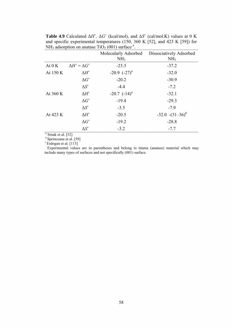
58

Table 4.9 Calculated ΔH˚, ΔG˚ (kcal/mol), and ΔS˚ (cal/mol.K) values at 0 K and specific experimental temperatures (150, 360 K [52], and 423 K [59]) for NH3 adsorption on anatase TiO2 (001) surface c.

Molecularly Adsorbed NH3

Dissociatively Adsorbed NH3

At 0 K ΔH˚ = ΔG˚ -23.3 -37.2 At 150 K ΔH˚ -20.9 (-27)a -32.0 ΔG˚ -20.2 -30.9 ΔS˚ -4.4 -7.2 At 360 K ΔH˚ -20.7 (-14)a -32.1 ΔG˚ -19.4 -29.3 ΔS˚ -3.5 -7.9 At 423 K ΔH˚ -20.5 -32.0 -(31–36)b ΔG˚ -19.2 -28.8 ΔS˚ -3.2 -7.7

a Srnak et al. [52] b Sprinceana et al. [59] c Erdogan et al. [113] Experimental values are in parentheses and belong to titania (anatase) material which may include many types of surfaces and not specifically (001) surface.

59

4.2 Periodic DFT Method

4.2.1 Water and Ammonia Adsorption on Anatase TiO2 (001) Slab Surface

4.2.1.1 Optimization of Slab Geometry

Optimized geometry of 4 layer p(2x2) anatase TiO2 (001) surface slab (Figure

4.13) is prepared by initially relaxing the crystal and then cutting the crystal along

(001) plane and placing a 15 Å vacuum layer above. The optimization of the bulk

crystal is carried out to determine the optimal lattice parameters, which are

calculated as a=b=3.822 Å, and c=9.670 Å. These values are in a good agreement

with the experimentally reported values, 3.785 Å and 9.514 Å [86].

Figure 4.13 Optimized slab geometry of 4 layer p(2x2) TiO2 anatase (001) slab.

60

4.2.1.2 Water Adsorption on Anatase TiO2 (001) Slab Surface


By using a slab geometry and a periodic DFT approach, water adsorption on

anatase TiO2 (001) surface is investigated. Molecular adsorption energy is

evaluated from total energy calculations as -14.62 kcal/mol. Figure 4.14 depicts

the optimized geometry of molecular H2O adsorption on anatase TiO2 (001) slab

model. For the molecular adsorption geometry, the distances between hydrogen

and oxygen of water molecule (Hw-Ow) and oxygen of water molecule and

fivefold coordinated titanium (Ow-Ti) are computed as 0.972 Å, and 2.171 Å,

respectively.

(a)

(b)

Figure 4.14 Optimized geometry of molecular H2O adsorption on anatase TiO2 (001) slab model. (a) Perspective view, (b) Top view.

61


For the case of dissociative adsorption mechanism, it is observed that water

molecule is dissociated on (001) anatase TiO2 slab surface with an exothermic

relative energy difference of 32.28 kcal/mol. For the optimized geometry of this

reaction (see Figure 4.15), the distances between hydrogen and oxygen of water

molecule (Hleft-Ow), hydrogen of water molecule and surface oxygen (Hright-Os),

and oxygen of water molecule and fivefold coordinated titanium (Ow-Ti) are

computed as 0.971 Å, 0.982 Å, and 1.892 Å respectively.

(a)

(b)

Figure 4.15 Optimized geometry of dissociative H2O adsorption on anatase TiO2 (001) slab model. (a) Perspective view, (b) Top view.

62


The calculated molecular and dissociative water adsorption energy values on

(001) anatase TiO2 surface are -14.62 kcal/mol and -32.28 kcal/mol, respectively.

These values are comparable with the available theoretical and experimental

literature data given in Table 4.10.

Table 4.10 A comparison of the calculated H2O adsorption energies (kcal/mol) on perfect anatase TiO2 (001) surface with the theoretical and experimental values in the literature.

Adsorption Energy Authors and References Method Molecular Dissociative Theoretical Fahmi and Minot 1994 [60] Periodic -14.34 -28.68 Vittadini et al. 1998 [13] PW:DFT-GGA Car-

Parrinello 1/2 ML-18.68 -33.21

Nair 2004 [64] DFT -18.64 -32.98 Jug et al. 2005 [62] MSINDO -23.90 -49.71 Arrouvel et al. 2004 [65] PW:DFT-GGA KS - -(24.1-39.4) Gong and Selloni 2005 [66] PW:DFT-GGA Car-

Parrinello 1/6 ML- -28.80

1/3 ML - -25.60 1/2 ML - -26.98 Onal et al. 2006 [70] DFT-B3LYP/6-31G** Relax -24.93 -54.00 Wahab et al. 2008 [69] MSINDO -17.69 -24.62 Erdogan et al. 2009 [113] ONIOM DFT/B3LYP/

6-31G**-MD/UFF -23.90 -33.67

Erdogan et al. 2009 [114] PW:DFT-GGA-PW91 -14.62 -32.28 Experimental Srnak et al. 1992 [52] TPD Anatase TiO2 -11, -18 Munuera et al. 1999 [53] TPD Anatase TiO2 -12

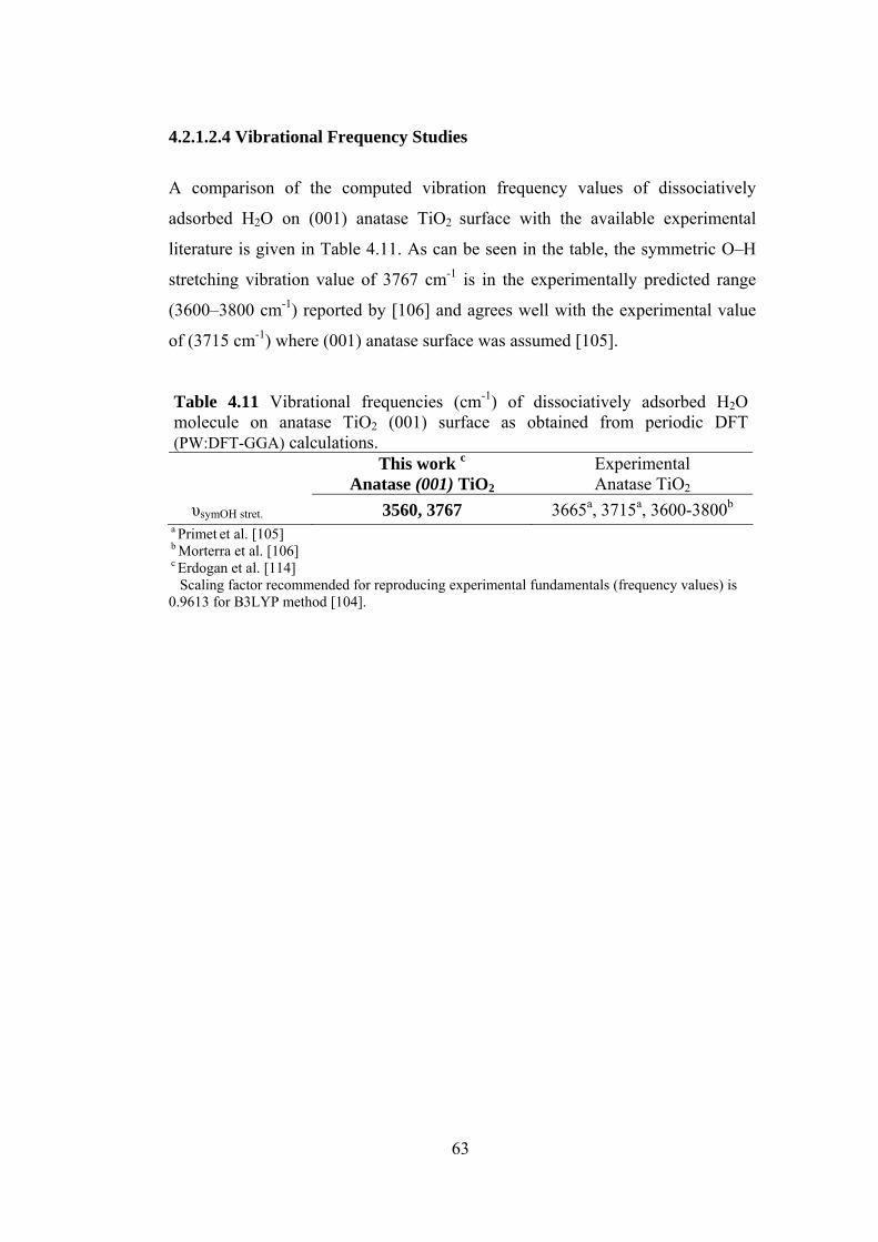
63


A comparison of the computed vibration frequency values of dissociatively

adsorbed H2O on (001) anatase TiO2 surface with the available experimental

literature is given in Table 4.11. As can be seen in the table, the symmetric O–H

stretching vibration value of 3767 cm-1 is in the experimentally predicted range

(3600–3800 cm-1) reported by [106] and agrees well with the experimental value

of (3715 cm-1) where (001) anatase surface was assumed [105].

a Primet et al. [105] b Morterra et al. [106] c Erdogan et al. [114] Scaling factor recommended for reproducing experimental fundamentals (frequency values) is 0.9613 for B3LYP method [104].

Table 4.11 Vibrational frequencies (cm-1) of dissociatively adsorbed H2O molecule on anatase TiO2 (001) surface as obtained from periodic DFT (PW:DFT-GGA) calculations.

This work c

Anatase (001) TiO2 Experimental Anatase TiO2

υsymOH stret. 3560, 3767 3665a, 3715a, 3600-3800b

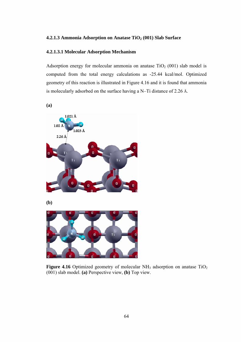
64

4.2.1.3 Ammonia Adsorption on Anatase TiO2 (001) Slab Surface


Adsorption energy for molecular ammonia on anatase TiO2 (001) slab model is

computed from the total energy calculations as -25.44 kcal/mol. Optimized

geometry of this reaction is illustrated in Figure 4.16 and it is found that ammonia

is molecularly adsorbed on the surface having a N–Ti distance of 2.26 Å.

(a)

(b)

Figure 4.16 Optimized geometry of molecular NH3 adsorption on anatase TiO2 (001) slab model. (a) Perspective view, (b) Top view.

65


A comparison of the computed adsorption energy values obtained from periodic

DFT method for NH3 adsorption on anatase TiO2 (001) surface with the available

literature is given in Table 4.12. Experimental TPD [52] and XRD, BET [59]

studies investigated NH3 adsorption on real TiO2 (anatase) catalyst surface and

therefore the slight deviation is reasonable in view of the fact that (001) surface is

minority in anatase as previously mentioned. However, molecular NH3 adsorption

energy value (-25.44 kcal/mol) obtained from periodic DFT calculations in this

study is quite comparable to the results of our preceding relaxed [70] and ONIOM

[113] cluster studies (-26.57 kcal/mol and -23.28 kcal/mol, respectively).

Table 4.12 A comparison of the calculated NH3 adsorption energies on perfect anatase TiO2 (001) surface with the theoretical and experimental values in the literature.

Adsorption Energy, kcal/mol Authors and References Method Molec. Dissoc. Act.Barr

Theoretical Calatayud et al. 2004 [71] PW:DFT-GGA KS -19.40 - Onal et al. 2006 [70] Relaxed cluster

DFT-B3LYP-6-31G** -26.57 -36.32 3.63

Erdogan et al. 2009 [113] ONIOM cluster DFT/B3LYP6-31G**-MD /UFF

-23.28 -37.17 2.68

Erdogan et al. 2009 [114] Periodic slab PW:DFT-GGA-PW91

-25.44 - -

Experimental Srnak et al. 1992 [52] TPD AnataseTiO2 -14, -27 Sprinceana et al. 1999 [59] XRD BET AnataseTiO2 -(31-36)


A vibration frequency study for ammonia adsorption is also performed and a

comparison of the vibrational properties of molecularly adsorbed NH3 molecule

on the (001) surface with the available experimental data reported for anatase

surfaces in general is given in Table 4.13. As this table shows, a symmetric

bending frequency value of 1094 cm−1 and asymmetric stretching frequency data

of (3510, 3535 cm−1) for molecular ammonia adsorption deviate significantly

from the experimental values of 1190, 1225 and 1215 cm−1 [107,108] and of 3400

66

cm−1 [109], respectively. The deviations from the experimental studies could be

expected since the particular surface of the TiO2 (anatase) on which NH3

adsorbed has not been reported in these studies and it is known that (001) surface

is minority in anatase. For the molecular ammonia adsorption asymmetric

bending (1573 cm-1, 1609 cm-1), and symmetric stretching (3385 cm-1), vibration

data are in agreement with the experimental values of (1599 cm-1 [107], 1600 cm-

1 [109]), and 3350 cm-1 [109], respectively.

Table 4.13 A comparison of the vibrational frequencies (cm-1) of molecularly adsorbed NH3 molecule on anatase TiO2 (001) surface as obtained from periodic DFT (PW:DFT-GGA) calculations with the experimental literature values e. Molecularly Ads. NH3

υasym HNH stret. 3510, 3535 (3400c)

υsym HNH stret. 3385 (3350c)

δasym HNH bend. 1573, 1609 (1599a, 1600c)

δsym HNH bend. 1094 (1190a, 1225a, 1215b) a Amores et al. [107] b Teramura et al. [108] c Schneider et al. [109] e Erdogan et al. [113] Scaling factor recommended for reproducing experimental fundamentals (frequency values) is 0.9613 for B3LYP method [104]. Experimental values are in parentheses and particular surface of the TiO2 (anatase) has not been reported.

67

CHAPTER 5

CONCLUSIONS

In this thesis, water adsorption on rutile TiO2 (110) surface represented by

partially relaxed Ti25O37 ONIOM cluster and water and ammonia adsorption on

anatase TiO2 (001) surface represented by partially relaxed Ti20O35 ONIOM

cluster models are investigated by means of quantum chemical calculations

employing ONIOM DFT/B3LYP/6-31G**-MM/UFF method provided in

Gaussian 03. Water and ammonia adsorption on anatase TiO2 (001) surface is

studied and compared by also performing periodic DFT calculations (PW:DFT-

GGA-PW91) using VASP code.

Firstly, ONIOM cluster calculations concerning water adsorption on rutile TiO2

(110) surface point out that the results obtained for molecular and dissociative

water adsorption energy values (-22.4 kcal/mol and -11.5 kcal/mol, respectively)

are quite similar to the most recent publication values (-18.4 kcal/mol vs. -13.4

kcal/mol, respectively) reported on this subject by Kamisaka et al. [51] using

VASP and exactly same to what Bandura et al. [46] obtained (-22.5 kcal/mol vs. -

11.5 kcal/mol, respectively) using Gaussian 98. Furthermore, if the diffusion of

the two OH groups is taken into consideration, we have calculated a reasonable

activation barrier value of 23.2 kcal/mol similar to what Wendt et al. [48]

obtained (27 kcal/mol) via periodic slab calculations in DACAPO. According to

such a high activation barrier, ONIOM cluster calculations indicate that

dissociative water adsorption on rutile TiO2 (110) is not favorable. There is a

good agreement with experimental literature regarding that molecular H2O

adsorption energy value obtained in this study (-22.4 kcal/mol) is in the range of

experimentally determined values -(14-24 kcal/mol). In fact, experimental studies

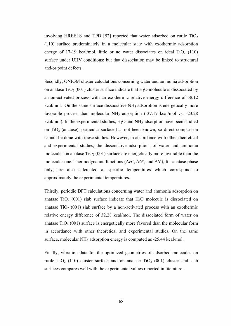
68

involving HREELS and TPD [52] reported that water adsorbed on rutile TiO2

(110) surface predominately in a molecular state with exothermic adsorption

energy of 17-19 kcal/mol, little or no water dissociates on ideal TiO2 (110)

surface under UHV conditions; but that dissociation may be linked to structural

and/or point defects.

Secondly, ONIOM cluster calculations concerning water and ammonia adsorption

on anatase TiO2 (001) cluster surface indicate that H2O molecule is dissociated by

a non-activated process with an exothermic relative energy difference of 58.12

kcal/mol. On the same surface dissociative NH3 adsorption is energetically more

favorable process than molecular NH3 adsorption (-37.17 kcal/mol vs. -23.28

kcal/mol). In the experimental studies, H2O and NH3 adsorption have been studied

on TiO2 (anatase), particular surface has not been known, so direct comparison

cannot be done with these studies. However, in accordance with other theoretical

and experimental studies, the dissociative adsorptions of water and ammonia

molecules on anatase TiO2 (001) surface are energetically more favorable than the

molecular one. Thermodynamic functions (ΔH˚, ΔG˚, and ΔS˚), for anatase phase

only, are also calculated at specific temperatures which correspond to

approximately the experimental temperatures.

Thirdly, periodic DFT calculations concerning water and ammonia adsorption on

anatase TiO2 (001) slab surface indicate that H2O molecule is dissociated on

anatase TiO2 (001) slab surface by a non-activated process with an exothermic

relative energy difference of 32.28 kcal/mol. The dissociated form of water on

anatase TiO2 (001) surface is energetically more favored than the molecular form

in accordance with other theoretical and experimental studies. On the same

surface, molecular NH3 adsorption energy is computed as -25.44 kcal/mol.

Finally, vibration data for the optimized geometries of adsorbed molecules on

rutile TiO2 (110) cluster surface and on anatase TiO2 (001) cluster and slab

surfaces compares well with the experimental values reported in literature.

69

REFERENCES

1. Emsley, J. Molecules at an Exhibition: portraits of intriguing materials in

everyday life; Oxford University Press; 1999.

2. Trengove, L.; William Gregor (1761–1817) discoverer of titanium; Annals of

Science 1972, 29, 36.

3. Kirk-Othmer Encyclopedia of Chemical Technology; 5th ed. Canada, John

Wiley & Sons, Inc., 2007, 25, 9.

4. Diebold, U. Surf Sci Reports 2003, 48, 53.

5. Samsonov, G.V. The Oxide Handbook; IFI/Plenum; New York; 1982.

6. Ulmann's Encyclopedia of Industrial Chemistry; 7th ed., New York, Wiley

Interscience; 2005, 20, 271.

7. Murray, J.L. Phase Diagrams of Binary Titanium Alloy; 1990, p.219.

8. Ramamoorthy, M.D.; Vanderbilt and R.D. King-Smith, Phys Rev B 1994, 49,

16721.

9. Satterfield, C.N. Heterogeneous Catalysis in Industrial Practice; 2nd ed.,

McGraw-Hill, New York, 1991.

10. Ohno, T.; Sarukawa, K.; Matsumura M. J Phys Chem B 2001, 105, 2417.

11. Hagfelt, A.; Gratzel, M. Chem Rev 1995, 95, 49.

12. Hadjivanov, K.I.; Klissurski, D.K. Chem Soc Rev 1996, 25, 61.

70

13. Vittadini, A.; Selloni, A.; Rotzinger, F.P.; Gratzel, M. Phys Rev Lett 1998,

81, 2954.

14. Lazzeri, M.; Vittadini, A.; Selloni, A. Phys Rev B 2001, 63, 155409.

15. Diebold, U.; Ruzycki, N.; Herman, G. S.; Selloni, A. Catal Today 2003, 85,

93.

16. Vittadini, A.; Casarin, M.; Selloni, A. Theor Chem Acc 2007, 117, 663.

17. Lazzeri, M.; Vittadini, A.; Selloni, A. Phys Rev B 2001, 63, 155409/1

18. Ando, M.; Kobayashi, T.; Haruta, M. Catal Today 1997, 36, 135.

19. Fujishima, A.; Honda, K. Nature 1972, 238, 37.

20. Dutta, P.K.; Ginwalla, A.; Hogg, B.; Patton, B.R.; Chwieroth, B; Liang, Z;

Gouma, P.; Mills, M.; Akbar, S. J Phys Chem 1999, 103, 4412.

21. Kronos International, 1996.

22. Phillips, L.G.; Barbano, D.M. J Dairy Sci 1997, 80, 2726.

23. Hewitt J. Cosmet Toiletries 1999, 114, 59.

24. Poulios, I.; Spathis, P.; Tsoumparis, P.; J Environ Sci Health 34, 1999, 1455.

25. Selhofer, H. Vacuum Thin Film 1999, 15.

26. Sambrano, J.R.; Andres, J.; Beltran, A.; Sensato, F.R.; Leite, E.R.; Stamato

F.M.L.G.; Longo E. Int J Quantum Chem 1997, 65, 625.

27. Mills, A.; Davies H.R.; Worsley, D. Chem Soc Rev 1993, 22, 417.

28. Maness, P.-C.; Smolinski, S.; Jacoby W.A. Appl Environ Microbiol 1999, 65,

4094.

71

29. Lausmaa, J.; Ask, M.; Rolander, U.; Kasemo, B. Mater Res Soc Symp Proc

1988, 110, 647.

30. Paz, Y.; Luo, Z.; Rabenberg, L.; Heller A. J Mater Res 1995, 10, 2842.

31. Garfunkel, E.; Gusev, E.; Vul (Eds.), A., Fundamental Aspects of Ultrathin

Dielectrics on Si-based Devices, NATO Science Series, Kluwer Academic

Publishers, Dordrecht, 1998.

32. Campbell, S.A.; Kim, H.-S.; Gilmer, D.C.; He, B.; Ma T.; Gladfelter, W.L.

IBM J Res Devlop 1999, 43, 383.

33. Matsumoto, Y.; Shono, T.; Hasegawa, T.; Fukumura, T.; Kawasaki, M.;

Ahmet, P.; Chikyow, T.; Koshihara, S.; Koinuma, H. Science 2001, 291, 854.

34. Bonhote, P.; Gogniat, E.; Grätzel, M.; Ashrit, P.V. Thin Solid Films 1999,

350, 269.

35. Kurtz, R.L.; Stockbauer, R.T.; Madey, E.; Roman, E.; de Segovia, J. L. Surf

Sci 1989, 218, 178.

36. Hugenschmidt, M.B.; Gamble, L.; Campbell, C.T. Surf Sci 1994, 302, 329.

37. Henderson, M.A. Surf Sci 1996, 355, 151.

38. Brinkley, D.; Dietrich, M.; Engel, T.; Farrall, P.; Gantner, G.; Schafer, A.;

Szuchmacher, A. Surf Sci 1998, 395, 292.

39. Brookes, I.M.; Muryn C.A.; Thornton, G. Phys Rev Lett 2001, 87, 266103/1.

40. Schaub, R.; Thostrup, P.; Lopez, N.; Lægsgaard, E.; Stensgaard, I.; Nørskov,

J.K.; Besenbacher, F. Phys Rev Lett 2001, 87, 266104.

41. Goniakowski, J.; Gillan, M.J. Surf Sci 1996, 350, 145.

42. Lindan, P.J.D.; Harrison, N.M.; Gillan, M. J Phys Rev Lett 1998, 80, 762.

72

43. Casarin M.; Maccato, C. J Phys Chem B 1998, 102, 10745.

44. Stefanovich, E.V.; Truong, T.N. Chem Phys Lett 1999, 299, 623.

45. Menetrey, M.; Markovits, M.A.; Minot, C. Surf Sci 2003, 524, 49.

46. Bandura, A.V.; Sykes, D.G.; Shapovalov, V.; Troung, T.N.; Kubicki, J.D.;

Evarestov, R.A. J Phys Chem B 2004, 108, 7844.

47. Wendt, S.; Shaub, R.; Matthiesen, J.; Vestergaard, E.K.; Wahlström, E.;

Rasmussen, M.D.; Thostrup, P; Molina, L.M.; Laegsgaarrd, E.; Stensgaard, I;

Hammer, B.; Besenbacher, F. Surf Sci 2005, 598, 226.

48. Wendt, S.; Matthiesen, J.; Shaub, R.; Vestergaard, E.K.; Laegsgaarrd, E.;

Besenbacher, F.; Hammer, B. Phys Rev Lett 2006, 96, 066107.

49. Lindan, P.J.D; Zhang, C. Phys Rev B 2005, 72, 075439.

50. Perron, H.; Vandenborre, J.; Domain, C.; Drot, R.; Roques, J.; Simoni, E.;

Ehrhardt, J.J.; Catalette, H. Surf Sci 2007, 601, 518.

51. Kamisaka H.; Yamashita, K.; Surf Sci 2007, 601, 4824.

52. Srnak, T.Z.; Dumesic, J.A.; Clausen, B.S.; Tornqvist, E.; Topsoe, N.Y. J Catal

1992, 135, 246.

53. Munuera, G.; Moreno, F.; Gonzales, F. A model for anatase TiO2 surfaces:

interpretation of some interface processes. Reactivity of solids; Proceedings of the

7th International Symposium Reaction Solids, Chapman & Hall, London 1972,

681.

54. Topsøe, N-Y.; Topsøe, H.; Dumesic, J.A. J Catal 1995, 151, 226.

55. Topsøe, N-Y.; Topsøe, H.; Dumesic, J.A. J Catal 1995, 151, 241.

73

56. Ramis, G.; Yi, L.; Busca, G.; Turco, M.; Kotur E.; Willey, R.J. J Catal 1995,

157, 523.

57. Ramis, G.; Yi, L.; Busca, G. Catal Today 1996, 28, 373.

58. Busca, G.; Lietti, L.; Ramis, G.; Berti, F. Appl Catal B 1998, 18, 1.

59. Sprinceana, D.; Caldararu, M.; Ionescu, N.I.; Auroux, A. J Therm Anal

Calorim 1999, 56, 109.

60. Fahmi, A.; Minot, C. Surf Sci 1994, 304, 343.

61. Bredow, T.; Jug, K. Surf Sci 1995, 327, 398.

62. Jug, K.; Nair, N.N.; Bredow, T. Surf Sci 2005, 596, 108.

63. Kachurovskaya, N.A.; Mikheeva, E.P.; Zhidomirov, G.M. J Mol Catal 2000,

178, 191.

64. Nair, N.N. Molecular Dynamics Investigation of Clusters and Solids, Ph.D.

Thesis; Theoretical Chemistry Institute, Hannover University, Germany, 2004.

65. Arrouvel C., Digne, M.; Breysse, M.; Toulhoat, H.; Raybaud, P. J Catal 2004,

222, 152.

66. Gong, X.-Q.; Selloni, A. J Phys Chem B Lett 2005, 109, 19560.

67. Barnard, A.S.; Zapol, P.; Curtiss, A. J Chem Theory Comput 2005, 1, 107.

68. Ignatchenko, A.; Nealon, D.G.; Dushane, R.; Humphries, K. J Mol Catal A

Chemical 2006, 256, 57.

69. Wahab, H.S.; Bredow, T.; Aliwi, M. Chem Phys 2008, 354 50.

70. Onal, I.; Soyer, S.; Senkan, S. Surf Sci 2006, 600, 2457.

71. Calatayud, M.; Mguig, B.; Minot, C. Surf Sci Reports 2004, 55, 169.

74

72. Young, D.C. Computational Chemistry; John Wiley & Sons, Inc., New York,

Chapter 27, 2001.

73. Hehre, J.W. A Guide to Molecular Mechanics and Quantum Calculations;

Wavefunction, Inc., Irvine, Chapter 2 and 3, 2003.

74. Vreven, T.; Byun, K.S.; Komaromi, I.; Dapprich, S.; Montgomery, J.A. Jr.;

Morokuma, K.; Frisch, M.J. J Chem Theory and Comput 2006, 2, 815.

75. Dapprich, S.; Komáromi, I.; Byun, K.S.; Morokuma, K.; Frisch, M.J. J Mol

Struct (Theochem) 1999, 46, 21.

76. Gaussian, Inc., www.gaussian.com/g_whitepap/oniom_technote.htm

Introduction to ONIOM, 11 Aug 2009.

77. Maseras, F.; Morokuma, K. J Comput Chem 1995, 16, 1170.

78. Derat, E.; Bouquant, J.; Humbel, S. J Mol Struct (THEOCHEM) 2003, 632,

61.

79. Warshel, A.; Levitt, M. J Mol Biol 1976, 103, 227.

80. Thery, V.; Rinaldi, D.; Rivail, J.L.; Maigret, B.; Ferenczy, G.G. J Comput

Chem 1994, 15, 269.

81. Reuter, N.; Dejaegere, A.; Maigret, B.; Karplus, M. J Phys Chem A 2000,

104, 1720.

82. Gao, J.; Amara, P.; Alhambra, C.; Field, M.J. J Phys Chem A 1998, 102,

4714.

83. Zhang, Y.K.; Lee, T.S.; Yang, W.T. J Chem Phys 1999, 110, 46.

84. DiLabio, G.A.; Hurley, M.M.; Christiansen, P.A. J Chem Phys 2002, 116,

9578.

75

85. Bakowies, D.; Thiel, W. J Phys Chem 1996, 100, 10580.

86. Wyckoff, R.W.G. Crystal structures; John Wiley & Sons, Inc., USA, 1963

Vol. I, pp. 250.

87. Gaussian 03, Revision D.01, Frisch, M.J.; Trucks, G.W.; Schlegel, H.B.;

Scuseria, G.E.; Robb, M.A.; Cheeseman, J.R.; J.A. Montgomery, Jr.,T. Vreven,

K.N. Kudin, J.C. Burant, J.M. Millam, S.S. Iyengar, J. Tomasi, V. Barone, B.

Mennucci, M. Cossi, G. Scalmani, N. Rega, G. A. Petersson, H. Nakatsuji, M.

Hada, M. Ehara, K. Toyota, R. Fukuda, J. Hasegawa, M. Ishida, T. Nakajima, Y.

H onda, O. Kitao, H . Nakai, M. Klene, X. Li, J.E.Knox, H .P. H ratchian,

J.B.Cross, C. Adamo, J. Jaramillo, R. Gomperts, R.E. Stratmann, O. Yazyev, A.J.

Austin, R. Cammi, C. Pomelli, J.W. Ochterski, P.Y. Ayala, K. Morokuma, G.A.

Voth, P. Salvador, J.J. Dannenberg, V.G. Zakrzewski, S. Dapprich, A.D. Daniels,

M.C. Strain, O. Farkas, D.K. Malick, A.D. Rabuck, K. Raghavachari, J.B.

Foresman, J.V. Ortiz, Q. Cui, A.G. Baboul, S. Clifford, J. Cioslowski, B.B.

Stefanov, G. Liu, A. Liashenko, P. Piskorz, I. Komaromi, R.L. Martin, D.J. Fox,

T. Keith, M.A. Al-Laham, C.Y. Peng, A. Nanayakkara, M. Challacombe, P.M.W.

Gill, B. Johnson, W. Chen, M.W. Wong, C. Gonzalez and J.A. Pople, Gaussian,

Inc., Pittsburgh PA, 2003.

88. Kohn W.; Sham, L.J. Phys Rev 1965, 140, A1133.

89. Becke, A.D. Phys Rev B 1988, 38, 3098.

90. Becke, A.D.; Roussel, M.R. Phys Rev A 1989, 39, 3761.

91. Lee, C.; Yang W.; Parr, R.G. Phys Rev B 1988, 37, 785.

92. Rappé, A.K.; Casewit, C.J.; Colwell, K.S.; Goddard III, W.A.; Skiff, W.M. J

Am Chem Soc 1992, 114, 10024.

93. Peng, C.; Schlegel, H.; Israel B. J Chem 1993, 33, 449.

76

94. McQuarrie, D.A.; Statistical Thermodynamics; Harper & Row Publishers;

NewYork, 1973.

95. Kresse G.; Furthmüller, J. Comp Mat Sci 1996, 6, 15.

96. Kresse G.; Joubert D. Phys Rev B 1999, 59, 1758.

97. Blöchl P.E. Phys Rev B 1994, 50, 17953.

98. Perdew J.P.; Chevary J. A.; Vosko S. H.; Jackson K.A.; Pederson M.R.; Singh

D.J.; Fiolhais C. Phys Rev B 1992, 46, 6671.

99. Wang Y.; Perdew J.P. Phys Rev B 1991, 44, 13298.

100. Lindsay, R.; Wander, A.; Ernst, A.; Montanari, B.; Thornton, G.; Harrison,

N.M. Phys Rev Lett 2005, 94, 246102.

101. Charlton, G.P.; Howes, B.C.; Nicklin, L.; Steadman, P.; Taylor, J.S.G.;

Muryn, C.A.; Harte, S.P.; Mercer, J.; McGrath, R.; Norman, D.; Turner, T.S.;

Thornton, G. Phys Rev Lett 1997, 78, 495.

102. Swamy, V.; Muscat, J.; Gale, J.D.; Harrison, N.M. Surf Sci 2002, 504, 115.

103. Allegretti, F.; O’Brien S.; Polcik, M.; Aayago, D.I.; Woodruff, D.P. Surf Sci

2006, 600, 1487.

104. Wong, M.W. Chem Phys Lett 1996, 256, 391.

105. Primet, M.; Pichat, P.; Mathieu, M-V. J Phys Chem 1971, 75, 1216.

106. Morterra, C. J Chem Soc Faraday Trans 1, 1988, 84, 1617.

107. Amores, J.M.G.; Escribano, V.S.; Ramis G.; Busca, G. Appl Catal B 1997,

13, 45.

108. Teramura, K.; Tanaka T.; Funabiki, T. Langmuir 2003, 19, 1209.

77

109. Schneider, H.; Tschudin, S.; Schneider, M.; Wokaun, A.; Baiker, A. J Catal

1994, 147, 5.

110. Lietti, L.; Ramis, G.; Berti, F.; Toledo, G.; Robba, D.; Busca, G.; Forzatti,

P. Catal Today 1998, 42, 101.

111. Pilar, F.L. Elementary Quantum Chemistry, Courier Dover Publications,

2001.

112. Erdogan, R.; Fellah, M.F.; Onal, I. “An ONIOM and DFT Study of Water

Adsorption on Rutile TiO2 (110) Cluster”, International Journal of Quantum

Chemistry, Accepted, DOI 10.1002/qua.22400.

113. Erdogan, R.; Onal, I. “An ONIOM and DFT Study of Water and Ammonia

Adsorption on Anatase TiO2 (001) Cluster”, International Journal of Quantum

Chemistry, Accepted, DOI 10.1002/qua.22501.

114. Erdogan, R.; Ozbek, O.; Onal, I. “A Periodic DFT Study of Water and

Ammonia Adsorption on Anatase TiO2 (001) Slab”, submitted to Surface Science.

78

APPENDIX A

INTRODUCTION BACKGROUND AND THEORY OF

COMPUTATIONAL QUANTUM CHEMISTRY

First Principles of Quantum Chemistry

In quantum chemistry, molecules are expressed in terms of interactions among

nuclei and electrons, and molecular geometry in terms of minimum energy

arrangements of nuclei [73]. All quantum chemical methods trace back to

Schrödinger equation, which for the special case of hydrogen atom may be solved

exactly. In generalized form of Schrödinger equation, the positions of nuclei and

electrons within a system are described by the wave function Ψ, which in

principal can be found by solving the molecular Schrödinger equation:

Ĥ Ψ = EΨ (A.1)

where Ĥ is the molecular Hamiltonian operator and E is an eigenvalue of Ĥ,

corresponding to total energy of the system. With the information of the positions

of the nuclei and electrons, the true values for all the molecular properties of

interest can be found. However, because the Schrödinger equation cannot be

solved exactly for multi-electron atoms and molecules system, approximation

methods are necessary. These approximations neglect or simplify a variety of

intra- and inter-atomic interactions.

Relativistic effects are neglected, as they only matter for very heavy atoms where

the electrons approach the speed of light. The molecular Hamiltonian operator can

then be written as: [111]

79

enn HVTH∧∧∧∧

++= (A.2)

where nT∧

represents the kinetic energy of the nuclei, nV∧

represents the potential

energy of nuclear-nuclear repulsions, and eH∧

represents all the terms involving

electrons:

eeenee HVTH −

∧

−

∧∧∧

++= (A.3)

Here eT∧

represents the kinetic energy of the electrons, enV −

∧

represents electron-

nucleus attraction, and eeH −

∧

represents the pair wise repulsion of electrons.

One way to simplify the Schrödinger equation for molecular systems is to assume

that the nuclei do not move thereby separating nT∧

and nV∧

from the problem. The

ability to study electrons in a field of stationary nuclei is based on the separation

of timescales; electrons respond very fast (the speed of light) to the slow

movements of nuclei. This is called Born-Oppenheimer approximation, and leads

to an “electronic” Schrödinger equation. This approximation is generally good,

although it does not hold when there are two electronic states with very similar

energies, as then even small perturbations, such as electron-nucleus interactions,

can be important.

The terms in the electronic Hamiltonian operator representing the kinetic energy

of the electrons ( eT∧

) and the electron-nucleus attraction ( enV −

∧

) act on one

electron at a time. The computational bottleneck is the pair wise repulsion of

electrons, eeH −

∧

, which depends on the coordinates of two electrons at the same

time.

The orbital approximation assumes that each electron moves in its own orbital.

The electron-electron interactions are de-coupled by treating the interaction

between one electron and all the others in an average way: each electron interacts

80

with the potential field caused by the average position of all the other electrons,

i.e. the electrons are uncorrelated. This reduces the eeH −

∧

term to an electric

potential term eV∧

. This approximation regarding uncorrelated electrons is a major

limitation, leading to a “correlation error”.

To find each electron orbital, the average electric potential due to all other

electron orbitals has to be known, but initially none of these are known. Trial

orbitals are used which are modified iteratively until a self-consistent field (SCF)

is found. This is known as the Hartree-Fock (HF) method, the most common ab-

initio method.

To find the wave function (Ψ) we express it as a linear combination of basis

functions, which can be thought of as atomic orbitals, and search for the set of

coefficients that gives the best combination. The HF method relies on the

Variation Principle, which states that the SCF with the lowest energy is the most

accurate approximation to the true wave function. The linear combination of basis

functions that leads to the SCF with the lowest energy is the best approximation.

Perturbation theory

Correlation can be added as a perturbation from the Hartree-Fock wave function.

This is called Møller-Plesset perturbation theory. In mapping the HF wave

function onto a perturbation theory formulation, HF becomes a first-order

perturbation. Thus, a minimal amount of correlation is added by using the second

order MP2 method. Third order (MP3) and fourth-order (MP4) calculations are

also common. Beyond MP2 the theory is not always convergent (precision does

not always improve), although computational cost always increases. These “post-

Hartree-Fock” calculations are very slow [72].

81

Coupled Cluster methods

Other post-Hartree-Fock methods for estimating electron correlation are the

coupled cluster (CC) methods. These allow for correlation between clusters, or

groups, of molecular orbitals. The abbreviations for these methods indicate the

size of the clusters considered: Singles – S, Doubles – D, Triples – T, Quadruples

– Q. For example, CCSD includes the correlation of electrons in each individual

orbital, as well as the pair wise correlation of electrons in every possible pair of

orbitals. This is roughly equivalent to what MP2 tries to estimate. CCSDT would

also include contributions from all possible groupings of three molecular orbitals.

The inclusion of all n levels of excitation for an n-electron system would give the

exact solution of the Schrödinger equation, within the given basis set. However,

because the number of possible groupings increases rapidly with the size of the

group, these methods scale poorly as the number of excitations considered is

increased, and it is very rare to exceed CCSDT. Parentheses in the acronym

indicate that an effect is estimated with perturbation theory, e.g. CCSD(T). This

particular level of theory is often called the “gold standard” of quantum chemistry

because of its high accuracy and feasible computational cost, although, scaling as

n7 with the number of basis functions, even this can be unaffordable for large

molecules.

Semi-empirical methods

Although they make approximations, ab-initio methods such as Hartree Fock use

no empirical information, except for fundamental constants such as the mass of an

electron. To calculate the repulsion between each electron and all the others, these

ab-initio methods require the computation of many integrals. In contrast, semi-

empirical methods neglect some integrals (the Zero Differential Overlap

assumption) and other integrals are replaced with parameters rather than being

calculated. These parameters have been determined empirically to fit the results to

experimental data. Semi-empirical methods are much faster than ab-initio

82

methods, but are less accurate and require the atoms of interest to be

parameterized in advance.

Density Functional Theory methods

Since the 1990s, Density Functional Theory (DFT) methods have often been used

instead of post-Hartree-Fock methods to calculate the electron correlation. These

methods work directly with electron density instead of with molecular wave

functions. The Hartree-Fock (HF) methods described above try to calculate the

exact energy of an approximate wave function. The energy is given exactly by the

Hamiltonian operator, but the wave function cannot be found without the mean-

field approximation. The wave function Ψ is a function of the positions (xi, yi, zi)

of each of the N electrons, and the energy E is a functional of Ψ:

Eexact (Ψ (x1, y1, z1, x2, y2, z2, . . . , xN, yN, zN)) (A.4)

Although the exact form of E(Ψ) is known, it cannot be solved without

approximation. In contrast, density functional methods calculate the energy, E,

directly from the electron density of the ground state, ρ, without the need to

approximate the wave function. However, the functional used to find the energy

from the electron density is an approximation. According to the Hohenberg-Kohn

theorem, the functional E(ρ) does exist in principle; its exact form however is

unknown. Instead, a variety of approximate functionals has been developed to

give good agreement with experimental data and detailed quantum calculations at

higher levels of theory. DFT calculations are therefore not strictly ab-initio.

In the Kohn-Sham formalism, the ground-state electronic energy, E, is written as

a sum of the kinetic energy, ET, the electron-nuclear interaction energy, EV, the

Coulomb energy, EJ, and the exchange/correlation energy, EXC.

E = ET + EV + EJ + EXC (A.5)

The preceding equation can be written in a more open way:

83

(A.6)

Notice that there are only three variables, compared to 3N for the HF method. For

large molecules, this makes DFT methods much faster than HF methods of

comparable accuracy. One disadvantage of DFT methods is the lack of systematic

improvement: with the HF methods one could continually add another term to the

perturbation or another excitation level to the cluster operator, until satisfied that

the change it makes is small; with DFT, although some functionals are probably

better than others, there is no way to guarantee convergence upon the true value

by changing functionals.

xcii

iA

iA

Aiii

iiie

Erdrdrr

rrrdrrR

ZrdrrE +−

+−

+∇−= ∫∑∫∑− 21211

2 )()(21)()()(

21 rr

rr

rrrr

rrrrr ρρρφφ

84

APPENDIX B

SAMPLE INPUT AND OUTPUT FILES

To represent the calculations those are done in this study:

Gaussian input and output files of vibrational frequency calculation of optimized

single H2O molecule are given in Table B.1 and Table B.2, respectively.

Gaussian input files of coordinate driving calculation and transition state

calculation of dissociative NH3 adsorption on anatase TiO2 (001) surface are

given in Table B.3 and Table B.4, respectively.

Finally, VASP files (POSCAR, K-POINTS, INCAR, and POTCAR) for volume

relaxation calculation of anatase TiO2 are given in Tables B.5-B.8, respectively.

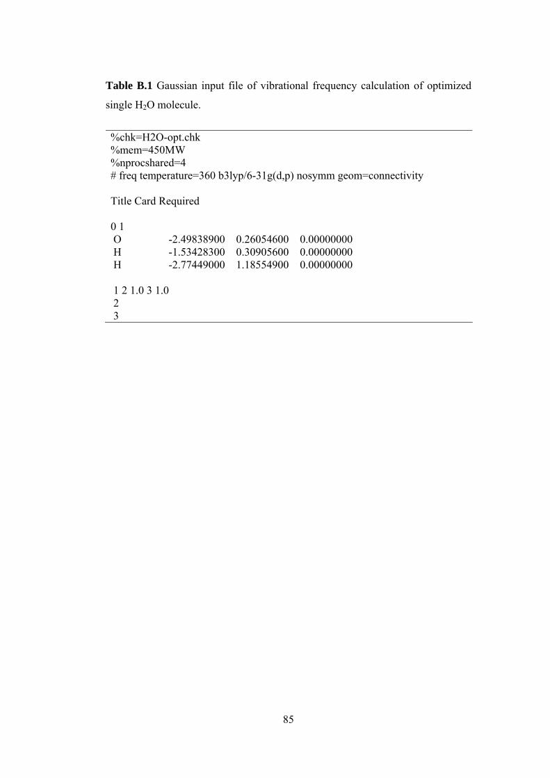
85

Table B.1 Gaussian input file of vibrational frequency calculation of optimized

single H2O molecule.

%chk=H2O-opt.chk %mem=450MW %nprocshared=4 # freq temperature=360 b3lyp/6-31g(d,p) nosymm geom=connectivity Title Card Required 0 1 O -2.49838900 0.26054600 0.00000000 H -1.53428300 0.30905600 0.00000000 H -2.77449000 1.18554900 0.00000000 1 2 1.0 3 1.0 2 3

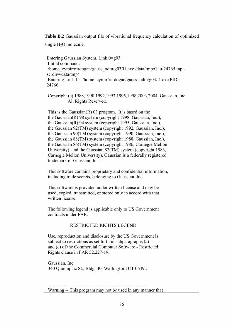
86

Table B.2 Gaussian output file of vibrational frequency calculation of optimized

single H2O molecule.

Entering Gaussian System, Link 0=g03 Initial command: /home_eymir/rerdogan/gauss_odtu/g03/l1.exe /data/tmp/Gau-24765.inp -scrdir=/data/tmp/ Entering Link 1 = /home_eymir/rerdogan/gauss_odtu/g03/l1.exe PID= 24766. Copyright (c) 1988,1990,1992,1993,1995,1998,2003,2004, Gaussian, Inc. All Rights Reserved. This is the Gaussian(R) 03 program. It is based on the the Gaussian(R) 98 system (copyright 1998, Gaussian, Inc.), the Gaussian(R) 94 system (copyright 1995, Gaussian, Inc.), the Gaussian 92(TM) system (copyright 1992, Gaussian, Inc.), the Gaussian 90(TM) system (copyright 1990, Gaussian, Inc.), the Gaussian 88(TM) system (copyright 1988, Gaussian, Inc.), the Gaussian 86(TM) system (copyright 1986, Carnegie Mellon University), and the Gaussian 82(TM) system (copyright 1983, Carnegie Mellon University). Gaussian is a federally registered trademark of Gaussian, Inc. This software contains proprietary and confidential information, including trade secrets, belonging to Gaussian, Inc. This software is provided under written license and may be used, copied, transmitted, or stored only in accord with that written license. The following legend is applicable only to US Government contracts under FAR: RESTRICTED RIGHTS LEGEND Use, reproduction and disclosure by the US Government is subject to restrictions as set forth in subparagraphs (a) and (c) of the Commercial Computer Software - Restricted Rights clause in FAR 52.227-19. Gaussian, Inc. 340 Quinnipiac St., Bldg. 40, Wallingford CT 06492 --------------------------------------------------------------- Warning -- This program may not be used in any manner that

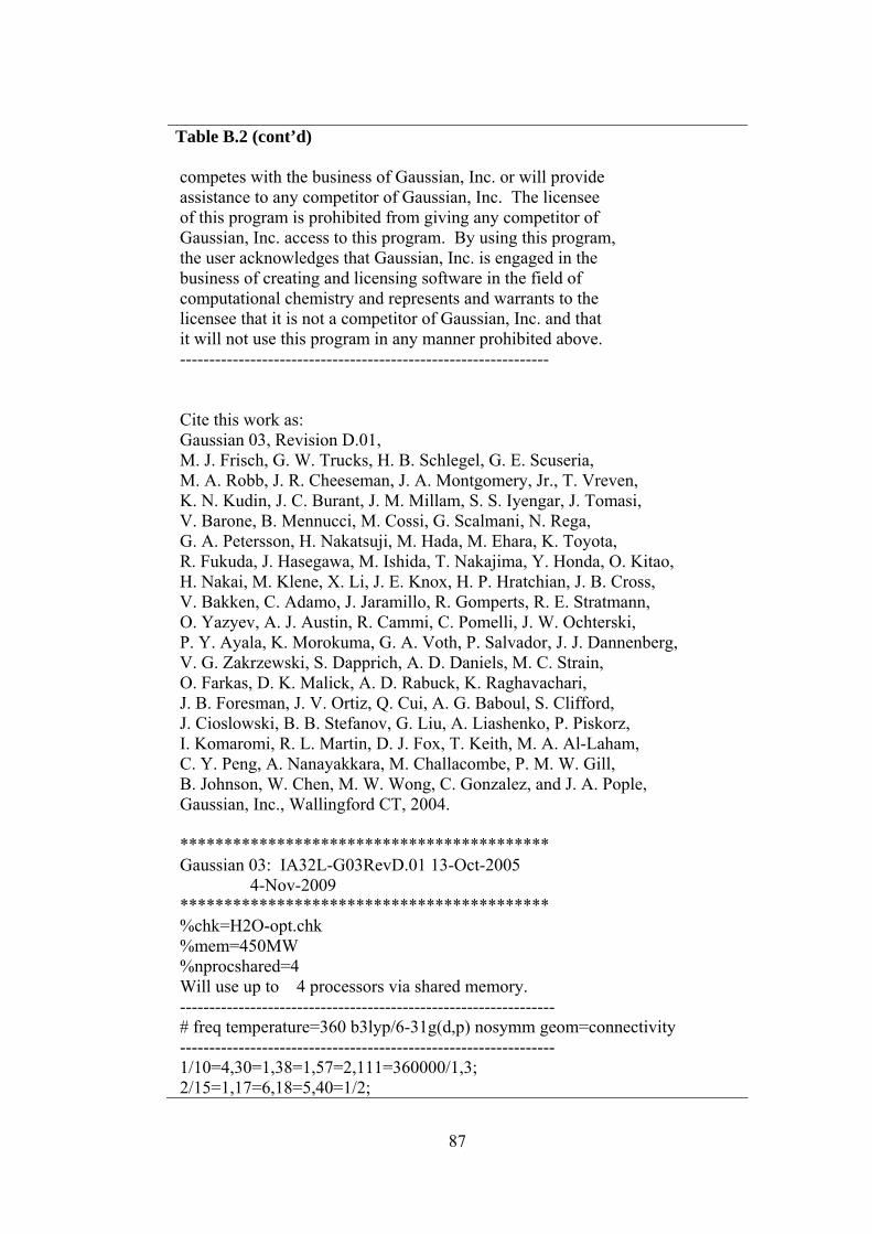
87

Table B.2 (cont’d) competes with the business of Gaussian, Inc. or will provide assistance to any competitor of Gaussian, Inc. The licensee of this program is prohibited from giving any competitor of Gaussian, Inc. access to this program. By using this program, the user acknowledges that Gaussian, Inc. is engaged in the business of creating and licensing software in the field of computational chemistry and represents and warrants to the licensee that it is not a competitor of Gaussian, Inc. and that it will not use this program in any manner prohibited above. --------------------------------------------------------------- Cite this work as: Gaussian 03, Revision D.01, M. J. Frisch, G. W. Trucks, H. B. Schlegel, G. E. Scuseria, M. A. Robb, J. R. Cheeseman, J. A. Montgomery, Jr., T. Vreven, K. N. Kudin, J. C. Burant, J. M. Millam, S. S. Iyengar, J. Tomasi, V. Barone, B. Mennucci, M. Cossi, G. Scalmani, N. Rega, G. A. Petersson, H. Nakatsuji, M. Hada, M. Ehara, K. Toyota, R. Fukuda, J. Hasegawa, M. Ishida, T. Nakajima, Y. Honda, O. Kitao, H. Nakai, M. Klene, X. Li, J. E. Knox, H. P. Hratchian, J. B. Cross, V. Bakken, C. Adamo, J. Jaramillo, R. Gomperts, R. E. Stratmann, O. Yazyev, A. J. Austin, R. Cammi, C. Pomelli, J. W. Ochterski, P. Y. Ayala, K. Morokuma, G. A. Voth, P. Salvador, J. J. Dannenberg, V. G. Zakrzewski, S. Dapprich, A. D. Daniels, M. C. Strain, O. Farkas, D. K. Malick, A. D. Rabuck, K. Raghavachari, J. B. Foresman, J. V. Ortiz, Q. Cui, A. G. Baboul, S. Clifford, J. Cioslowski, B. B. Stefanov, G. Liu, A. Liashenko, P. Piskorz, I. Komaromi, R. L. Martin, D. J. Fox, T. Keith, M. A. Al-Laham, C. Y. Peng, A. Nanayakkara, M. Challacombe, P. M. W. Gill, B. Johnson, W. Chen, M. W. Wong, C. Gonzalez, and J. A. Pople, Gaussian, Inc., Wallingford CT, 2004. ****************************************** Gaussian 03: IA32L-G03RevD.01 13-Oct-2005 4-Nov-2009 ****************************************** %chk=H2O-opt.chk %mem=450MW %nprocshared=4 Will use up to 4 processors via shared memory. ---------------------------------------------------------------- # freq temperature=360 b3lyp/6-31g(d,p) nosymm geom=connectivity ---------------------------------------------------------------- 1/10=4,30=1,38=1,57=2,111=360000/1,3; 2/15=1,17=6,18=5,40=1/2;

88

Table B.2 (cont’d) 3/5=1,6=6,7=101,11=2,16=1,25=1,30=1,74=-5/1,2,3; 4//1; 5/5=2,38=5/2; 8/6=4,10=90,11=11/1; 11/6=1,8=1,9=11,15=111,16=1,31=1/1,2,10; 10/6=1,31=1/2; 6/7=2,8=2,9=2,10=2,18=1,28=1/1; 7/8=1,10=1,25=1,30=1/1,2,3,16; 1/10=4,30=1/3; 99//99; ------------------- Title Card Required ------------------- Symbolic Z-matrix: Charge = 0 Multiplicity = 1 O -2.49839 0.26055 0. H -1.53428 0.30906 0. H -2.77449 1.18555 0. GradGradGradGradGradGradGradGradGradGradGradGradGradGradGradGrad Berny optimization. Initialization pass. Trust Radius=3.00D-01 FncErr=1.00D-07 GrdErr=1.00D-07 Number of steps in this run= 2 maximum allowed number of steps= 2. GradGradGradGradGradGradGradGradGradGradGradGradGradGradGradGrad Input orientation: --------------------------------------------------------------------- Center Atomic Atomic Coordinates (Angstroms) Number Number Type X Y Z --------------------------------------------------------------------- 1 8 0 -2.498389 0.260546 0.000000 2 1 0 -1.534283 0.309056 0.000000 3 1 0 -2.774490 1.185549 0.000000 --------------------------------------------------------------------- Distance matrix (angstroms): 1 2 3 1 O 0.000000 2 H 0.965326 0.000000 3 H 0.965330 1.518668 0.000000 Symmetry turned off by external request. Stoichiometry H2O Framework group CS[SG(H2O)]

89

Table B.2 (cont’d) Deg. of freedom 3 Full point group CS Rotational constants (GHZ): 794.6747273 434.8467193 281.0538190 Standard basis: 6-31G(d,p) (6D, 7F) Integral buffers will be 262144 words long. Raffenetti 2 integral format. Two-electron integral symmetry is turned off. 25 basis functions, 42 primitive gaussians, 25 cartesian basis functions 5 alpha electrons 5 beta electrons nuclear repulsion energy 9.1193905001 Hartrees. NAtoms= 3 NActive= 3 NUniq= 3 SFac= 7.50D-01 NAtFMM= 80 NAOKFM=F Big=F One-electron integrals computed using PRISM. NBasis= 25 RedAO= T NBF= 25 NBsUse= 25 1.00D-06 NBFU= 25 Harris functional with IExCor= 402 diagonalized for initial guess. ExpMin= 1.61D-01 ExpMax= 5.48D+03 ExpMxC= 8.25D+02 IAcc=1 IRadAn= 1 AccDes= 1.00D-06 HarFok: IExCor= 402 AccDes= 1.00D-06 IRadAn= 1 IDoV=1 ScaDFX= 1.000000 1.000000 1.000000 1.000000 Requested convergence on RMS density matrix=1.00D-08 within 128 cycles. Requested convergence on MAX density matrix=1.00D-06. Requested convergence on energy=1.00D-06. No special actions if energy rises. Keep R1 integrals in memory in canonical form, NReq= 1771596. Integral accuracy reduced to 1.0D-05 until final iterations. Initial convergence to 1.0D-05 achieved. Increase integral accuracy. SCF Done: E(RB+HF-LYP) = -76.4197371213 A.U. after 9 cycles Convg = 0.4819D-08 -V/T = 2.0078 S**2 = 0.0000 Range of M.O.s used for correlation: 1 25 NBasis= 25 NAE= 5 NBE= 5 NFC= 0 NFV= 0 NROrb= 25 NOA= 5 NOB= 5 NVA= 20 NVB= 20 Symmetrizing basis deriv contribution to polar: IMax=3 JMax=2 DiffMx= 0.00D+00 G2DrvN: will do 4 centers at a time, making 1 passes doing MaxLOS=2. FoFDir/FoFCou used for L=0 through L=2. DoAtom=TTT Differentiating once with respect to electric field. with respect to dipole field. Differentiating once with respect to nuclear coordinates. Store integrals in memory, NReq= 873587. There are 12 degrees of freedom in the 1st order CPHF. 9 vectors were produced by pass 0. AX will form 9 AO Fock derivatives at one time. 9 vectors were produced by pass 1.

90

Table B.2 (cont’d) 9 vectors were produced by pass 2. 9 vectors were produced by pass 3. 7 vectors were produced by pass 4. 4 vectors were produced by pass 5. Inv2: IOpt= 1 Iter= 1 AM= 4.70D-16 Conv= 1.00D-12. Inverted reduced A of dimension 47 with in-core refinement. Isotropic polarizability for W= 0.000000 5.35 Bohr**3. End of Minotr Frequency-dependent properties file 721 does not exist. **************************************************************** Population analysis using the SCF density. **************************************************************** Alpha occ. eigenvalues -- -19.13801 -0.99731 -0.51498 -0.37102 -0.29196 Alpha virt. eigenvalues -- 0.06534 0.15122 0.75684 0.80551 0.89135 Alpha virt. eigenvalues -- 0.89353 1.01557 1.17538 1.52951 1.53765 Alpha virt. eigenvalues -- 1.64363 2.23869 2.26821 2.45005 2.64098 Alpha virt. eigenvalues -- 2.66677 3.02783 3.30718 3.53153 3.69289 Condensed to atoms (all electrons): 1 2 3 1 O 8.041971 0.283940 0.283940 2 H 0.283940 0.439602 -0.028468 3 H 0.283940 -0.028468 0.439603 Mulliken atomic charges: 1 1 O -0.609851 2 H 0.304925 3 H 0.304926 Sum of Mulliken charges= 0.00000 Atomic charges with hydrogens summed into heavy atoms: 1 1 O 0.000000 2 H 0.000000 3 H 0.000000 Sum of Mulliken charges= 0.00000 APT atomic charges: 1 1 O -0.481533 2 H 0.240765 3 H 0.240768 Sum of APT charges= 0.00000 APT Atomic charges with hydrogens summed into heavy atoms: 1 1 O 0.000000

91

Table B.2 (cont’d) 2 H 0.000000 3 H 0.000000 Sum of APT charges= 0.00000 Electronic spatial extent (au): <R**2>= 237.8347 Charge= 0.0000 electrons Dipole moment (field-independent basis, Debye): X= 1.1791 Y= 1.6684 Z= 0.0000 Tot= 2.0429 Quadrupole moment (field-independent basis, Debye-Ang): XX= -10.5855 YY= -4.2224 ZZ= -7.1378 XY= -4.4226 XZ= 0.0000 YZ= 0.0000 Traceless Quadrupole moment (field-independent basis, Debye-Ang): XX= -3.2703 YY= 3.0929 ZZ= 0.1774 XY= -4.4226 XZ= 0.0000 YZ= 0.0000 Octapole moment (field-independent basis, Debye-Ang**2): XXX= 57.8778 YYY= -3.5677 ZZZ= 0.0000 XYY= 9.6006 XXY= 10.2208 XXZ= 0.0000 XZZ= 17.5139 YZZ= -2.3114 YYZ= 0.0000 XYZ= 0.0000 Hexadecapole moment (field-independent basis, Debye-Ang**3): XXXX= -260.9400 YYYY= -7.3490 ZZZZ= -5.1254 XXXY= -19.4142 XXXZ= 0.0000 YYYX= 7.9614 YYYZ= 0.0000 ZZZX= 0.0000 ZZZY= 0.0000 XXYY= -24.3018 XXZZ= -45.0390 YYZZ= -2.7529 XXYZ= 0.0000 YYXZ= 0.0000 ZZXY= 5.7578 N-N= 9.119390500099D+00 E-N=-1.988497441065D+02 KE= 7.582636293535D+01 Exact polarizability: 6.860 -0.920 6.209 0.000 0.000 2.994 Approx polarizability: 8.445 -1.035 7.712 0.000 0.000 3.295 Full mass-weighted force constant matrix: Low frequencies --- -44.9705 -33.5976 -0.0012 -0.0005 0.0010 32.9914 Low frequencies --- 1664.8733 3799.6572 3912.8604 Diagonal vibrational polarizability: 0.2521340 0.4691807 0.0000000 Harmonic frequencies (cm**-1), IR intensities (KM/Mole), Raman scattering activities (A**4/AMU), depolarization ratios for plane and unpolarized incident light, reduced masses (AMU), force constants (mDyne/A), and normal coordinates: 1 2 3 A' A' A' Frequencies -- 1664.8733 3799.6572 3912.8604 Red. masses -- 1.0827 1.0452 1.0811 Frc consts -- 1.7681 8.8905 9.7522 IR Inten -- 70.3204 1.6388 20.2112 Atom AN X Y Z X Y Z X Y Z 1 8 0.04 0.06 0.00 -0.03 -0.04 0.00 0.06 -0.04 0.00 2 1 0.03 -0.70 0.00 0.70 -0.01 0.00 -0.71 -0.04 0.00 3 1 -0.67 -0.21 0.00 -0.25 0.66 0.00 -0.20 0.67 0.00

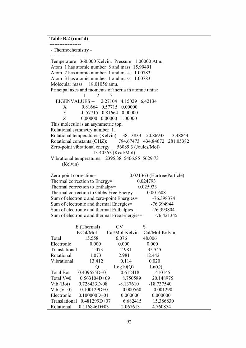
92

Table B.2 (cont’d) ------------------- - Thermochemistry - ------------------- Temperature 360.000 Kelvin. Pressure 1.00000 Atm. Atom 1 has atomic number 8 and mass 15.99491 Atom 2 has atomic number 1 and mass 1.00783 Atom 3 has atomic number 1 and mass 1.00783 Molecular mass: 18.01056 amu. Principal axes and moments of inertia in atomic units: 1 2 3 EIGENVALUES -- 2.27104 4.15029 6.42134 X 0.81664 0.57715 0.00000 Y -0.57715 0.81664 0.00000 Z 0.00000 0.00000 1.00000 This molecule is an asymmetric top. Rotational symmetry number 1. Rotational temperatures (Kelvin) 38.13833 20.86933 13.48844 Rotational constants (GHZ): 794.67473 434.84672 281.05382 Zero-point vibrational energy 56089.3 (Joules/Mol) 13.40565 (Kcal/Mol) Vibrational temperatures: 2395.38 5466.85 5629.73 (Kelvin) Zero-point correction= 0.021363 (Hartree/Particle) Thermal correction to Energy= 0.024793 Thermal correction to Enthalpy= 0.025933 Thermal correction to Gibbs Free Energy= -0.001608 Sum of electronic and zero-point Energies= -76.398374 Sum of electronic and thermal Energies= -76.394944 Sum of electronic and thermal Enthalpies= -76.393804 Sum of electronic and thermal Free Energies= -76.421345 E (Thermal) CV S KCal/Mol Cal/Mol-Kelvin Cal/Mol-Kelvin Total 15.558 6.076 48.006 Electronic 0.000 0.000 0.000 Translational 1.073 2.981 35.545 Rotational 1.073 2.981 12.442 Vibrational 13.412 0.114 0.020 Q Log10(Q) Ln(Q) Total Bot 0.409655D+01 0.612418 1.410145 Total V=0 0.563104D+09 8.750589 20.148975 Vib (Bot) 0.728433D-08 -8.137610 -18.737540 Vib (V=0) 0.100129D+01 0.000560 0.001290 Electronic 0.100000D+01 0.000000 0.000000 Translational 0.481299D+07 6.682415 15.386830 Rotational 0.116846D+03 2.067613 4.760854

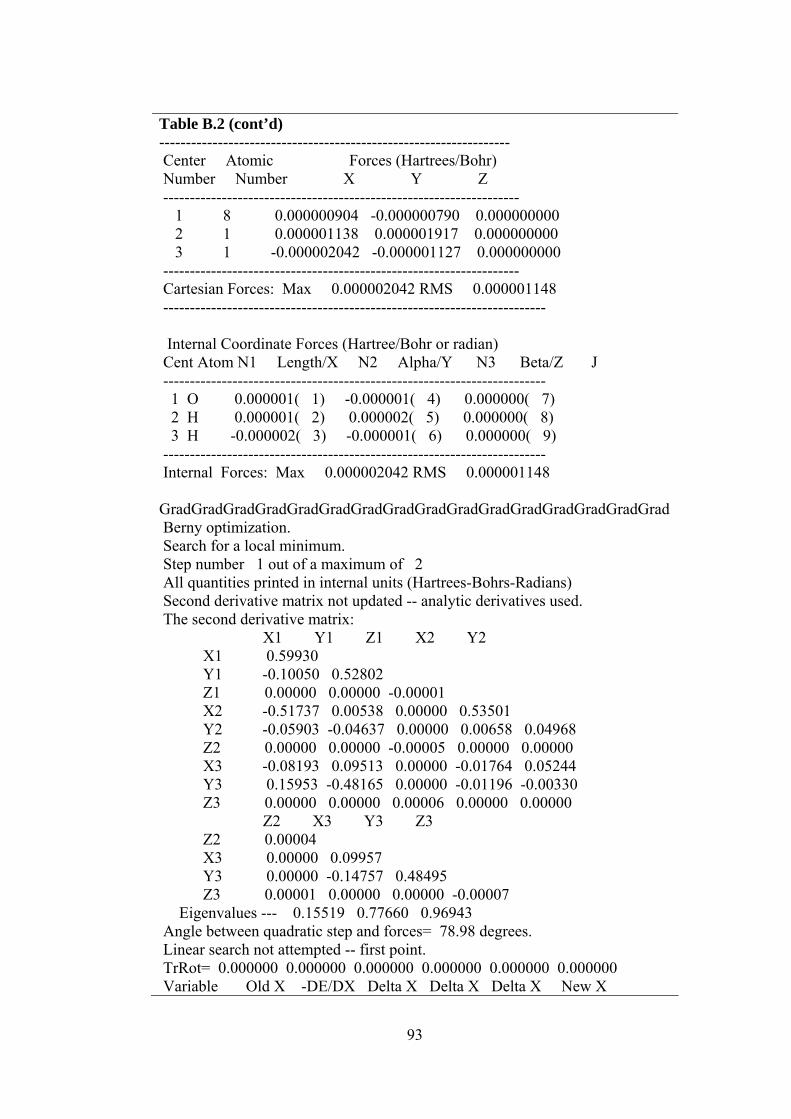
93

Table B.2 (cont’d) ------------------------------------------------------------------ Center Atomic Forces (Hartrees/Bohr) Number Number X Y Z ------------------------------------------------------------------- 1 8 0.000000904 -0.000000790 0.000000000 2 1 0.000001138 0.000001917 0.000000000 3 1 -0.000002042 -0.000001127 0.000000000 ------------------------------------------------------------------- Cartesian Forces: Max 0.000002042 RMS 0.000001148 ------------------------------------------------------------------------ Internal Coordinate Forces (Hartree/Bohr or radian) Cent Atom N1 Length/X N2 Alpha/Y N3 Beta/Z J ------------------------------------------------------------------------ 1 O 0.000001( 1) -0.000001( 4) 0.000000( 7) 2 H 0.000001( 2) 0.000002( 5) 0.000000( 8) 3 H -0.000002( 3) -0.000001( 6) 0.000000( 9) ------------------------------------------------------------------------ Internal Forces: Max 0.000002042 RMS 0.000001148 GradGradGradGradGradGradGradGradGradGradGradGradGradGradGradGrad Berny optimization. Search for a local minimum. Step number 1 out of a maximum of 2 All quantities printed in internal units (Hartrees-Bohrs-Radians) Second derivative matrix not updated -- analytic derivatives used. The second derivative matrix: X1 Y1 Z1 X2 Y2 X1 0.59930 Y1 -0.10050 0.52802 Z1 0.00000 0.00000 -0.00001 X2 -0.51737 0.00538 0.00000 0.53501 Y2 -0.05903 -0.04637 0.00000 0.00658 0.04968 Z2 0.00000 0.00000 -0.00005 0.00000 0.00000 X3 -0.08193 0.09513 0.00000 -0.01764 0.05244 Y3 0.15953 -0.48165 0.00000 -0.01196 -0.00330 Z3 0.00000 0.00000 0.00006 0.00000 0.00000 Z2 X3 Y3 Z3 Z2 0.00004 X3 0.00000 0.09957 Y3 0.00000 -0.14757 0.48495 Z3 0.00001 0.00000 0.00000 -0.00007 Eigenvalues --- 0.15519 0.77660 0.96943 Angle between quadratic step and forces= 78.98 degrees. Linear search not attempted -- first point. TrRot= 0.000000 0.000000 0.000000 0.000000 0.000000 0.000000 Variable Old X -DE/DX Delta X Delta X Delta X New X

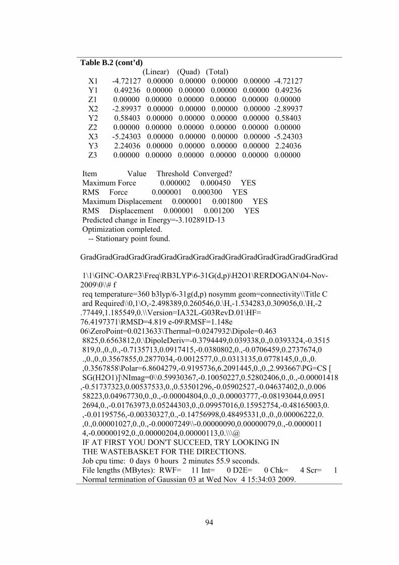
94

Table B.2 (cont’d) (Linear) (Quad) (Total) X1 -4.72127 0.00000 0.00000 0.00000 0.00000 -4.72127 Y1 0.49236 0.00000 0.00000 0.00000 0.00000 0.49236 Z1 0.00000 0.00000 0.00000 0.00000 0.00000 0.00000 X2 -2.89937 0.00000 0.00000 0.00000 0.00000 -2.89937 Y2 0.58403 0.00000 0.00000 0.00000 0.00000 0.58403 Z2 0.00000 0.00000 0.00000 0.00000 0.00000 0.00000 X3 -5.24303 0.00000 0.00000 0.00000 0.00000 -5.24303 Y3 2.24036 0.00000 0.00000 0.00000 0.00000 2.24036 Z3 0.00000 0.00000 0.00000 0.00000 0.00000 0.00000 Item Value Threshold Converged? Maximum Force 0.000002 0.000450 YES RMS Force 0.000001 0.000300 YES Maximum Displacement 0.000001 0.001800 YES RMS Displacement 0.000001 0.001200 YES Predicted change in Energy=-3.102891D-13 Optimization completed. -- Stationary point found. GradGradGradGradGradGradGradGradGradGradGradGradGradGradGradGrad 1\1\GINC-OAR23\Freq\RB3LYP\6-31G(d,p)\H2O1\RERDOGAN\04-Nov-2009\0\\# f req temperature=360 b3lyp/6-31g(d,p) nosymm geom=connectivity\\Title C ard Required\\0,1\O,-2.498389,0.260546,0.\H,-1.534283,0.309056,0.\H,-2 .77449,1.185549,0.\\Version=IA32L-G03RevD.01\HF= 76.4197371\RMSD=4.819 e-09\RMSF=1.148e 06\ZeroPoint=0.0213633\Thermal=0.0247932\Dipole=0.463 8825,0.6563812,0.\DipoleDeriv=-0.3794449,0.039338,0.,0.0393324,-0.3515 819,0.,0.,0.,-0.7135713,0.0917415,-0.0380802,0.,-0.0706459,0.2737674,0 .,0.,0.,0.3567855,0.2877034,-0.0012577,0.,0.0313135,0.0778145,0.,0.,0. ,0.3567858\Polar=6.8604279,-0.9195736,6.2091445,0.,0.,2.993667\PG=CS [ SG(H2O1)]\NImag=0\\0.59930367,-0.10050227,0.52802406,0.,0.,-0.00001418 ,-0.51737323,0.00537533,0.,0.53501296,-0.05902527,-0.04637402,0.,0.006 58223,0.04967730,0.,0.,-0.00004804,0.,0.,0.00003777,-0.08193044,0.0951 2694,0.,-0.01763973,0.05244303,0.,0.09957016,0.15952754,-0.48165003,0. ,-0.01195756,-0.00330327,0.,-0.14756998,0.48495331,0.,0.,0.00006222,0. ,0.,0.00001027,0.,0.,-0.00007249\\-0.00000090,0.00000079,0.,-0.0000011 4,-0.00000192,0.,0.00000204,0.00000113,0.\\\@ IF AT FIRST YOU DON'T SUCCEED, TRY LOOKING IN THE WASTEBASKET FOR THE DIRECTIONS. Job cpu time: 0 days 0 hours 2 minutes 55.9 seconds. File lengths (MBytes): RWF= 11 Int= 0 D2E= 0 Chk= 4 Scr= 1 Normal termination of Gaussian 03 at Wed Nov 4 15:34:03 2009.

95

Table B.3 Gaussian input file for coordinate driving calculation of dissociative

NH3 adsorption on anatase TiO2 (001) surface. (The output “relative energy

profile” is shown in Figure 4.10).

%chk=anatase-3x-3y-3z-001-2ti.chk %mem=400MW %nprocshared=2 # opt=(modredundant,loose,maxcycle=1000) oniom(b3lyp/6-31g(d,p):uff) nosymm geom=connectivity scf=(maxcycle=2000,conver=4) Title Card Required 0 1 0 1 0 1 Ti- -1 -3.780277 -5.678187 -0.870925 L Ti-Ti3+4 -1 -1.887277 -5.678187 1.507075 L O-O_3 -1 -3.780277 -5.678187 1.094075 L O-O_3 -1 -1.887277 -5.678187 -0.458925 L O-O_3 -1 -1.887277 -3.786187 1.920075 L Ti-Ti3+4 -1 0.004723 -5.678187 -0.870925 L H-H_21 0 Ti-Ti3+4 -1 1.897723 -5.678187 1.507075 L O-O_3 -1 0.004723 -5.678187 1.094075 L O-O_3 -1 1.897723 -5.678187 -0.458925 L O-O_3 -1 1.897723 -3.786187 1.920075 L Ti- -1 3.789723 -5.678187 -0.870925 L O-O_3 -1 3.789723 -5.678187 1.094075 L Ti-Ti3+4 -1 -3.780277 -1.893187 -0.870925 L H-H_17 0 Ti- -1 -1.887277 -1.893187 1.507075 L H-H_22 0 O-O_3 -1 -3.780277 -3.786187 -1.283925 L O-O_3 -1 -3.780277 -1.893187 1.094075 L O-O_3 -1 -1.887277 -1.893187 -0.458925 H O-O_3 -1 -1.887277 -0.001187 1.920075 L Ti- 0 0.004090 -1.920835 -0.889064 H Ti- -1 1.897723 -1.893187 1.507075 L H-H_22 0 O-O_3 -1 0.004723 -3.786187 -1.283925 H O-O_3 -1 0.004723 -1.893187 1.094075 H O-O_3 -1 1.897723 -1.893187 -0.458925 H O-O_3 -1 1.897723 -0.001187 1.920075 L Ti-Ti3+4 -1 3.789723 -1.893187 -0.870925 L H-H_22 0 O-O_3 -1 3.789723 -3.786187 -1.283925 L O-O_3 -1 3.789723 -1.893187 1.094075 L Ti-Ti3+4 -1 -3.780277 1.891813 -0.870925 L H-H_32 0 Ti- -1 -1.887277 1.891813 1.507075 L H-H_37 0 O-O_3 -1 -3.780277 -0.001187 -1.283925 L O-O_3 -1 -3.780277 1.891813 1.094075 L O-O_3 -1 -1.887277 1.891813 -0.458925 H O-O_3 -1 -1.887277 3.783813 1.920075 L Ti- 0 0.004453 1.899084 -0.834613 H Ti- -1 1.897723 1.891813 1.507075 L H-H_37 0 O-O_3 0 0.002857 0.112321 -1.284824 H O-O_3 -1 0.004723 1.891813 1.094075 H O-O_3 -1 1.897723 1.891813 -0.458925 H O-O_3 -1 1.897723 3.783813 1.920075 L

96

Table B.3 (cont’d) Ti-Ti3+4 -1 3.789723 1.891813 -0.870925 L H-H_38 0 O-O_3 -1 3.789723 -0.001187 -1.283925 L O-O_3 -1 3.789723 1.891813 1.094075 L Ti- -1 -3.780277 5.676813 -0.870925 L Ti-Ti3+4 -1 -1.887277 5.676813 1.507075 L O-O_3 -1 -3.780277 3.783813 -1.283925 L O-O_3 -1 -3.780277 5.676813 1.094075 L O-O_3 -1 -1.887277 5.676813 -0.458925 L Ti-Ti3+4 -1 0.004723 5.676813 -0.870925 L H-H_50 0 Ti-Ti3+4 -1 1.897723 5.676813 1.507075 L O-O_3 -1 0.004723 3.783813 -1.283925 H O-O_3 -1 0.004723 5.676813 1.094075 L O-O_3 -1 1.897723 5.676813 -0.458925 L Ti- -1 3.789723 5.676813 -0.870925 L O-O_3 -1 3.789723 3.783813 -1.283925 L O-O_3 -1 3.789723 5.676813 1.094075 L N-N_3 0 0.076971 -1.773815 -3.107569 H H-H_ 0 0.011323 -2.685768 -3.551398 H H-H_ 0 0.953207 -1.318295 -3.348198 H H-H_ 0 -0.679341 -1.160896 -3.399117 H 1 3 1.0 4 1.0 15 1.0 2 3 1.0 4 1.0 5 1.0 8 1.0 3 4 6 1.0 5 14 1.0 6 8 1.0 9 1.0 21 1.0 7 8 1.0 9 1.0 10 1.0 12 1.0 8 9 11 1.0 10 20 1.0 11 12 1.0 26 1.0 12 13 15 1.0 16 1.0 17 1.0 30 1.0 14 16 1.0 17 1.0 18 1.0 22 1.0 15 16 17 19 1.0 18 29 1.0 19 21 1.0 22 1.0 23 1.0 36 1.0 20 22 1.0 23 1.0 24 1.0 27 1.0 21 22 23 25 1.0 24 35 1.0 25 26 1.0 27 1.0 41 1.0 26 27 28 30 1.0 31 1.0 32 1.0 45 1.0 29 31 1.0 32 1.0 33 1.0 37 1.0 30 31 32 34 1.0 33 44 1.0 34 36 1.0 37 1.0 38 1.0 50 1.0 35 37 1.0 38 1.0 39 1.0 42 1.0

97

Table B.3 (cont’d) 36 37 38 40 1.0 39 49 1.0 40 41 1.0 42 1.0 54 1.0 41 42 43 45 1.0 46 1.0 47 1.0 44 46 1.0 47 1.0 51 1.0 45 46 47 48 1.0 48 50 1.0 51 1.0 52 1.0 49 51 1.0 52 1.0 55 1.0 50 51 52 53 1.0 53 54 1.0 55 1.0 54 55 56 57 1.0 58 1.0 59 1.0 57 58 59 B 59 36 S 40 -0.041000

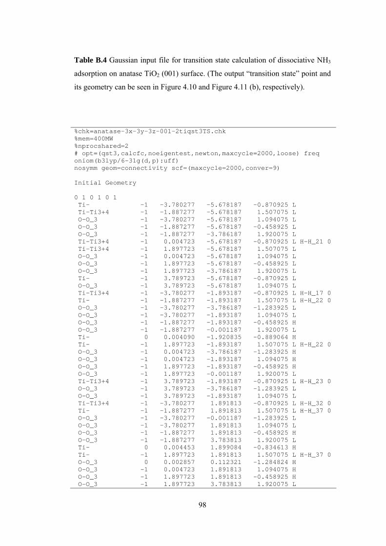
98

Table B.4 Gaussian input file for transition state calculation of dissociative NH3

adsorption on anatase TiO2 (001) surface. (The output “transition state” point and

its geometry can be seen in Figure 4.10 and Figure 4.11 (b), respectively).

%chk=anatase-3x-3y-3z-001-2tiqst3TS.chk %mem=400MW %nprocshared=2 # opt=(qst3,calcfc,noeigentest,newton,maxcycle=2000,loose) freq oniom(b3lyp/6-31g(d,p):uff) nosymm geom=connectivity scf=(maxcycle=2000,conver=9) Initial Geometry 0 1 0 1 0 1 Ti- -1 -3.780277 -5.678187 -0.870925 L Ti-Ti3+4 -1 -1.887277 -5.678187 1.507075 L O-O_3 -1 -3.780277 -5.678187 1.094075 L O-O_3 -1 -1.887277 -5.678187 -0.458925 L O-O_3 -1 -1.887277 -3.786187 1.920075 L Ti-Ti3+4 -1 0.004723 -5.678187 -0.870925 L H-H_21 0 Ti-Ti3+4 -1 1.897723 -5.678187 1.507075 L O-O_3 -1 0.004723 -5.678187 1.094075 L O-O_3 -1 1.897723 -5.678187 -0.458925 L O-O_3 -1 1.897723 -3.786187 1.920075 L Ti- -1 3.789723 -5.678187 -0.870925 L O-O_3 -1 3.789723 -5.678187 1.094075 L Ti-Ti3+4 -1 -3.780277 -1.893187 -0.870925 L H-H_17 0 Ti- -1 -1.887277 -1.893187 1.507075 L H-H_22 0 O-O_3 -1 -3.780277 -3.786187 -1.283925 L O-O_3 -1 -3.780277 -1.893187 1.094075 L O-O_3 -1 -1.887277 -1.893187 -0.458925 H O-O_3 -1 -1.887277 -0.001187 1.920075 L Ti- 0 0.004090 -1.920835 -0.889064 H Ti- -1 1.897723 -1.893187 1.507075 L H-H_22 0 O-O_3 -1 0.004723 -3.786187 -1.283925 H O-O_3 -1 0.004723 -1.893187 1.094075 H O-O_3 -1 1.897723 -1.893187 -0.458925 H O-O_3 -1 1.897723 -0.001187 1.920075 L Ti-Ti3+4 -1 3.789723 -1.893187 -0.870925 L H-H_23 0 O-O_3 -1 3.789723 -3.786187 -1.283925 L O-O_3 -1 3.789723 -1.893187 1.094075 L Ti-Ti3+4 -1 -3.780277 1.891813 -0.870925 L H-H_32 0 Ti- -1 -1.887277 1.891813 1.507075 L H-H_37 0 O-O_3 -1 -3.780277 -0.001187 -1.283925 L O-O_3 -1 -3.780277 1.891813 1.094075 L O-O_3 -1 -1.887277 1.891813 -0.458925 H O-O_3 -1 -1.887277 3.783813 1.920075 L Ti- 0 0.004453 1.899084 -0.834613 H Ti- -1 1.897723 1.891813 1.507075 L H-H_37 0 O-O_3 0 0.002857 0.112321 -1.284824 H O-O_3 -1 0.004723 1.891813 1.094075 H O-O_3 -1 1.897723 1.891813 -0.458925 H O-O_3 -1 1.897723 3.783813 1.920075 L

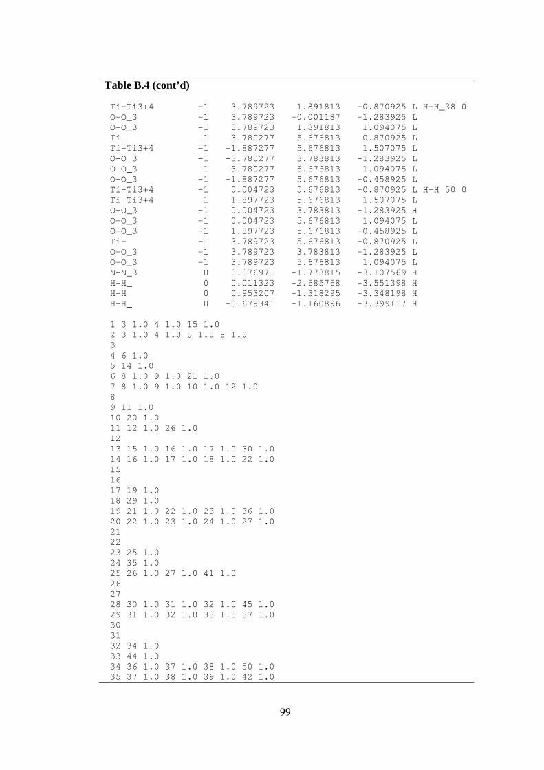
99

Table B.4 (cont’d) Ti-Ti3+4 -1 3.789723 1.891813 -0.870925 L H-H_38 0 O-O_3 -1 3.789723 -0.001187 -1.283925 L O-O_3 -1 3.789723 1.891813 1.094075 L Ti- -1 -3.780277 5.676813 -0.870925 L Ti-Ti3+4 -1 -1.887277 5.676813 1.507075 L O-O_3 -1 -3.780277 3.783813 -1.283925 L O-O_3 -1 -3.780277 5.676813 1.094075 L O-O_3 -1 -1.887277 5.676813 -0.458925 L Ti-Ti3+4 -1 0.004723 5.676813 -0.870925 L H-H_50 0 Ti-Ti3+4 -1 1.897723 5.676813 1.507075 L O-O_3 -1 0.004723 3.783813 -1.283925 H O-O_3 -1 0.004723 5.676813 1.094075 L O-O_3 -1 1.897723 5.676813 -0.458925 L Ti- -1 3.789723 5.676813 -0.870925 L O-O_3 -1 3.789723 3.783813 -1.283925 L O-O_3 -1 3.789723 5.676813 1.094075 L N-N_3 0 0.076971 -1.773815 -3.107569 H H-H_ 0 0.011323 -2.685768 -3.551398 H H-H_ 0 0.953207 -1.318295 -3.348198 H H-H_ 0 -0.679341 -1.160896 -3.399117 H 1 3 1.0 4 1.0 15 1.0 2 3 1.0 4 1.0 5 1.0 8 1.0 3 4 6 1.0 5 14 1.0 6 8 1.0 9 1.0 21 1.0 7 8 1.0 9 1.0 10 1.0 12 1.0 8 9 11 1.0 10 20 1.0 11 12 1.0 26 1.0 12 13 15 1.0 16 1.0 17 1.0 30 1.0 14 16 1.0 17 1.0 18 1.0 22 1.0 15 16 17 19 1.0 18 29 1.0 19 21 1.0 22 1.0 23 1.0 36 1.0 20 22 1.0 23 1.0 24 1.0 27 1.0 21 22 23 25 1.0 24 35 1.0 25 26 1.0 27 1.0 41 1.0 26 27 28 30 1.0 31 1.0 32 1.0 45 1.0 29 31 1.0 32 1.0 33 1.0 37 1.0 30 31 32 34 1.0 33 44 1.0 34 36 1.0 37 1.0 38 1.0 50 1.0 35 37 1.0 38 1.0 39 1.0 42 1.0

100

Table B.4 (cont’d) 36 37 38 40 1.0 39 49 1.0 40 41 1.0 42 1.0 54 1.0 41 42 43 45 1.0 46 1.0 47 1.0 44 46 1.0 47 1.0 51 1.0 45 46 47 48 1.0 48 50 1.0 51 1.0 52 1.0 49 51 1.0 52 1.0 55 1.0 50 51 52 53 1.0 53 54 1.0 55 1.0 54 55 56 57 1.0 58 1.0 59 1.0 57 58 59 Equilibrium Geometry 0 1 0 1 0 1 Ti- -1 -3.780277 -5.678187 -0.870925 L Ti-Ti3+4 -1 -1.887277 -5.678187 1.507075 L O-O_3 -1 -3.780277 -5.678187 1.094075 L O-O_3 -1 -1.887277 -5.678187 -0.458925 L O-O_3 -1 -1.887277 -3.786187 1.920075 L Ti-Ti3+4 -1 0.004723 -5.678187 -0.870925 L H-H_21 0 Ti-Ti3+4 -1 1.897723 -5.678187 1.507075 L O-O_3 -1 0.004723 -5.678187 1.094075 L O-O_3 -1 1.897723 -5.678187 -0.458925 L O-O_3 -1 1.897723 -3.786187 1.920075 L Ti- -1 3.789723 -5.678187 -0.870925 L O-O_3 -1 3.789723 -5.678187 1.094075 L Ti-Ti3+4 -1 -3.780277 -1.893187 -0.870925 L H-H_17 0 Ti- -1 -1.887277 -1.893187 1.507075 L H-H_22 0 O-O_3 -1 -3.780277 -3.786187 -1.283925 L O-O_3 -1 -3.780277 -1.893187 1.094075 L O-O_3 -1 -1.887277 -1.893187 -0.458925 H O-O_3 -1 -1.887277 -0.001187 1.920075 L Ti- 0 0.005075 -2.122250 -0.861672 H Ti- -1 1.897723 -1.893187 1.507075 L H-H_22 0 O-O_3 -1 0.004723 -3.786187 -1.283925 H O-O_3 -1 0.004723 -1.893187 1.094075 H O-O_3 -1 1.897723 -1.893187 -0.458925 H O-O_3 -1 1.897723 -0.001187 1.920075 L Ti-Ti3+4 -1 3.789723 -1.893187 -0.870925 L H-H_23 0 O-O_3 -1 3.789723 -3.786187 -1.283925 L O-O_3 -1 3.789723 -1.893187 1.094075 L Ti-Ti3+4 -1 -3.780277 1.891813 -0.870925 L H-H_32 0

101

Table B.4 (cont’d) Ti- -1 -1.887277 1.891813 1.507075 L H-H_37 0 O-O_3 -1 -3.780277 -0.001187 -1.283925 L O-O_3 -1 -3.780277 1.891813 1.094075 L O-O_3 -1 -1.887277 1.891813 -0.458925 H O-O_3 -1 -1.887277 3.783813 1.920075 L Ti- 0 0.005327 2.103799 -0.912863 H Ti- -1 1.897723 1.891813 1.507075 L H-H_37 0 O-O_3 0 0.007377 1.341705 -2.503577 H O-O_3 -1 0.004723 1.891813 1.094075 H O-O_3 -1 1.897723 1.891813 -0.458925 H O-O_3 -1 1.897723 3.783813 1.920075 L Ti-Ti3+4 -1 3.789723 1.891813 -0.870925 L H-H_38 0 O-O_3 -1 3.789723 -0.001187 -1.283925 L O-O_3 -1 3.789723 1.891813 1.094075 L Ti- -1 -3.780277 5.676813 -0.870925 L Ti-Ti3+4 -1 -1.887277 5.676813 1.507075 L O-O_3 -1 -3.780277 3.783813 -1.283925 L O-O_3 -1 -3.780277 5.676813 1.094075 L O-O_3 -1 -1.887277 5.676813 -0.458925 L Ti-Ti3+4 -1 0.004723 5.676813 -0.870925 L H-H_50 0 Ti-Ti3+4 -1 1.897723 5.676813 1.507075 L O-O_3 -1 0.004723 3.783813 -1.283925 H O-O_3 -1 0.004723 5.676813 1.094075 L O-O_3 -1 1.897723 5.676813 -0.458925 L Ti- -1 3.789723 5.676813 -0.870925 L O-O_3 -1 3.789723 3.783813 -1.283925 L O-O_3 -1 3.789723 5.676813 1.094075 L N-N_3 0 -0.002786 -1.278629 -2.620168 H H-H_ 0 -0.841903 -1.469158 -3.164268 H H-H_ 0 0.811048 -1.502694 -3.189412 H H-H_ 0 0.014603 0.337241 -2.587325 H 1 3 1.0 4 1.0 15 1.0 2 3 1.0 4 1.0 5 1.0 8 1.0 3 4 6 1.0 5 14 1.0 6 8 1.0 9 1.0 21 1.0 7 8 1.0 9 1.0 10 1.0 12 1.0 8 9 11 1.0 10 20 1.0 11 12 1.0 26 1.0 12 13 15 1.0 16 1.0 17 1.0 30 1.0 14 16 1.0 17 1.0 18 1.0 22 1.0 15 16 17 19 1.0 18 29 1.0 19 21 1.0 22 1.0 23 1.0 56 1.0 20 22 1.0 23 1.0 24 1.0 27 1.0 21 22 23 25 1.0 24 35 1.0

102

Table B.4 (cont’d) 25 26 1.0 27 1.0 41 1.0 26 27 28 30 1.0 31 1.0 32 1.0 45 1.0 29 31 1.0 32 1.0 33 1.0 37 1.0 30 31 32 34 1.0 33 44 1.0 34 36 1.0 37 1.0 38 1.0 50 1.0 35 37 1.0 38 1.0 39 1.0 42 1.0 36 59 1.0 37 38 40 1.0 39 49 1.0 40 41 1.0 42 1.0 54 1.0 41 42 43 45 1.0 46 1.0 47 1.0 44 46 1.0 47 1.0 51 1.0 45 46 47 48 1.0 48 50 1.0 51 1.0 52 1.0 49 51 1.0 52 1.0 55 1.0 50 51 52 53 1.0 53 54 1.0 55 1.0 54 55 56 57 1.0 58 1.0 57 58 59 Approx TS 0 1 0 1 0 1 Ti- -1 -3.780277 -5.678187 -0.870925 L Ti-Ti3+4 -1 -1.887277 -5.678187 1.507075 L O-O_3 -1 -3.780277 -5.678187 1.094075 L O-O_3 -1 -1.887277 -5.678187 -0.458925 L O-O_3 -1 -1.887277 -3.786187 1.920075 L Ti-Ti3+4 -1 0.004723 -5.678187 -0.870925 L H-H_21 0 Ti-Ti3+4 -1 1.897723 -5.678187 1.507075 L O-O_3 -1 0.004723 -5.678187 1.094075 L O-O_3 -1 1.897723 -5.678187 -0.458925 L O-O_3 -1 1.897723 -3.786187 1.920075 L Ti- -1 3.789723 -5.678187 -0.870925 L O-O_3 -1 3.789723 -5.678187 1.094075 L Ti-Ti3+4 -1 -3.780277 -1.893187 -0.870925 L H-H_17 0 Ti- -1 -1.887277 -1.893187 1.507075 L H-H_22 0 O-O_3 -1 -3.780277 -3.786187 -1.283925 L O-O_3 -1 -3.780277 -1.893187 1.094075 L O-O_3 -1 -1.887277 -1.893187 -0.458925 H

103

Table B.4 (cont’d) O-O_3 -1 -1.887277 -0.001187 1.920075 L Ti-Ti3+4 0 0.007294 -2.045197 -0.876354 H Ti- -1 1.897723 -1.893187 1.507075 L H-H_22 0 O-O_3 -1 0.004723 -3.786187 -1.283925 H O-O_3 -1 0.004723 -1.893187 1.094075 H O-O_3 -1 1.897723 -1.893187 -0.458925 H O-O_3 -1 1.897723 -0.001187 1.920075 L Ti-Ti3+4 -1 3.789723 -1.893187 -0.870925 L H-H_23 0 O-O_3 -1 3.789723 -3.786187 -1.283925 L O-O_3 -1 3.789723 -1.893187 1.094075 L Ti-Ti3+4 -1 -3.780277 1.891813 -0.870925 L H-H_32 0 Ti- -1 -1.887277 1.891813 1.507075 L H-H_37 0 O-O_3 -1 -3.780277 -0.001187 -1.283925 L O-O_3 -1 -3.780277 1.891813 1.094075 L O-O_3 -1 -1.887277 1.891813 -0.458925 H O-O_3 -1 -1.887277 3.783813 1.920075 L Ti- 0 0.000964 1.960949 -0.847360 H Ti- -1 1.897723 1.891813 1.507075 L H-H_37 0 O-O_3 0 -0.003030 0.343073 -1.587548 H O-O_3 -1 0.004723 1.891813 1.094075 H O-O_3 -1 1.897723 1.891813 -0.458925 H O-O_3 -1 1.897723 3.783813 1.920075 L Ti-Ti3+4 -1 3.789723 1.891813 -0.870925 L H-H_38 0 O-O_3 -1 3.789723 -0.001187 -1.283925 L O-O_3 -1 3.789723 1.891813 1.094075 L Ti- -1 -3.780277 5.676813 -0.870925 L Ti-Ti3+4 -1 -1.887277 5.676813 1.507075 L O-O_3 -1 -3.780277 3.783813 -1.283925 L O-O_3 -1 -3.780277 5.676813 1.094075 L O-O_3 -1 -1.887277 5.676813 -0.458925 L Ti-Ti3+4 -1 0.004723 5.676813 -0.870925 L H-H_50 0 Ti-Ti3+4 -1 1.897723 5.676813 1.507075 L O-O_3 -1 0.004723 3.783813 -1.283925 H O-O_3 -1 0.004723 5.676813 1.094075 L O-O_3 -1 1.897723 5.676813 -0.458925 L Ti- -1 3.789723 5.676813 -0.870925 L O-O_3 -1 3.789723 3.783813 -1.283925 L O-O_3 -1 3.789723 5.676813 1.094075 L N-N_3 0 0.109526 -1.600169 -2.986096 H H-H_ 0 -0.664397 -1.957554 -3.537849 H H-H_ 0 0.987674 -1.875248 -3.413828 H H-H_ 0 0.056940 -0.536394 -2.691360 H 1 3 1.0 4 1.0 15 1.0 2 3 1.0 4 1.0 5 1.0 8 1.0 3 4 6 1.0 5 14 1.0 6 8 1.0 9 1.0 21 1.0 7 8 1.0 9 1.0 10 1.0 12 1.0 8 9 11 1.0 10 20 1.0 11 12 1.0 26 1.0 12 13 15 1.0 16 1.0 17 1.0 30 1.0

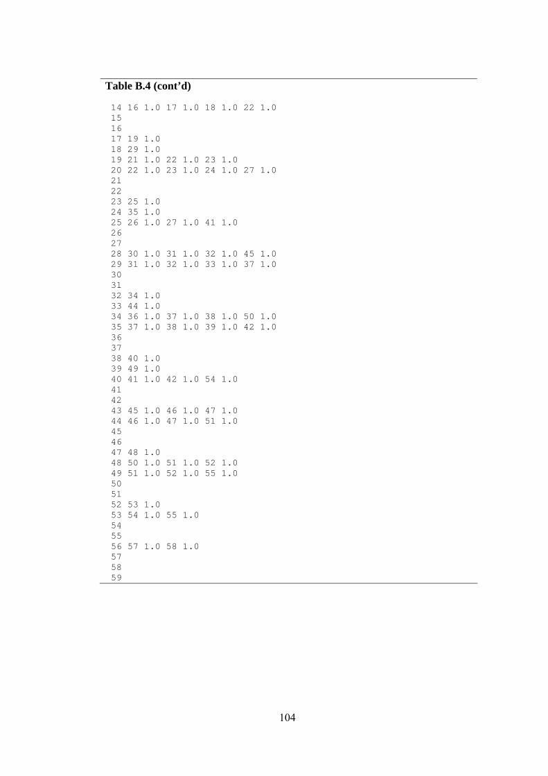
104

Table B.4 (cont’d) 14 16 1.0 17 1.0 18 1.0 22 1.0 15 16 17 19 1.0 18 29 1.0 19 21 1.0 22 1.0 23 1.0 20 22 1.0 23 1.0 24 1.0 27 1.0 21 22 23 25 1.0 24 35 1.0 25 26 1.0 27 1.0 41 1.0 26 27 28 30 1.0 31 1.0 32 1.0 45 1.0 29 31 1.0 32 1.0 33 1.0 37 1.0 30 31 32 34 1.0 33 44 1.0 34 36 1.0 37 1.0 38 1.0 50 1.0 35 37 1.0 38 1.0 39 1.0 42 1.0 36 37 38 40 1.0 39 49 1.0 40 41 1.0 42 1.0 54 1.0 41 42 43 45 1.0 46 1.0 47 1.0 44 46 1.0 47 1.0 51 1.0 45 46 47 48 1.0 48 50 1.0 51 1.0 52 1.0 49 51 1.0 52 1.0 55 1.0 50 51 52 53 1.0 53 54 1.0 55 1.0 54 55 56 57 1.0 58 1.0 57 58 59

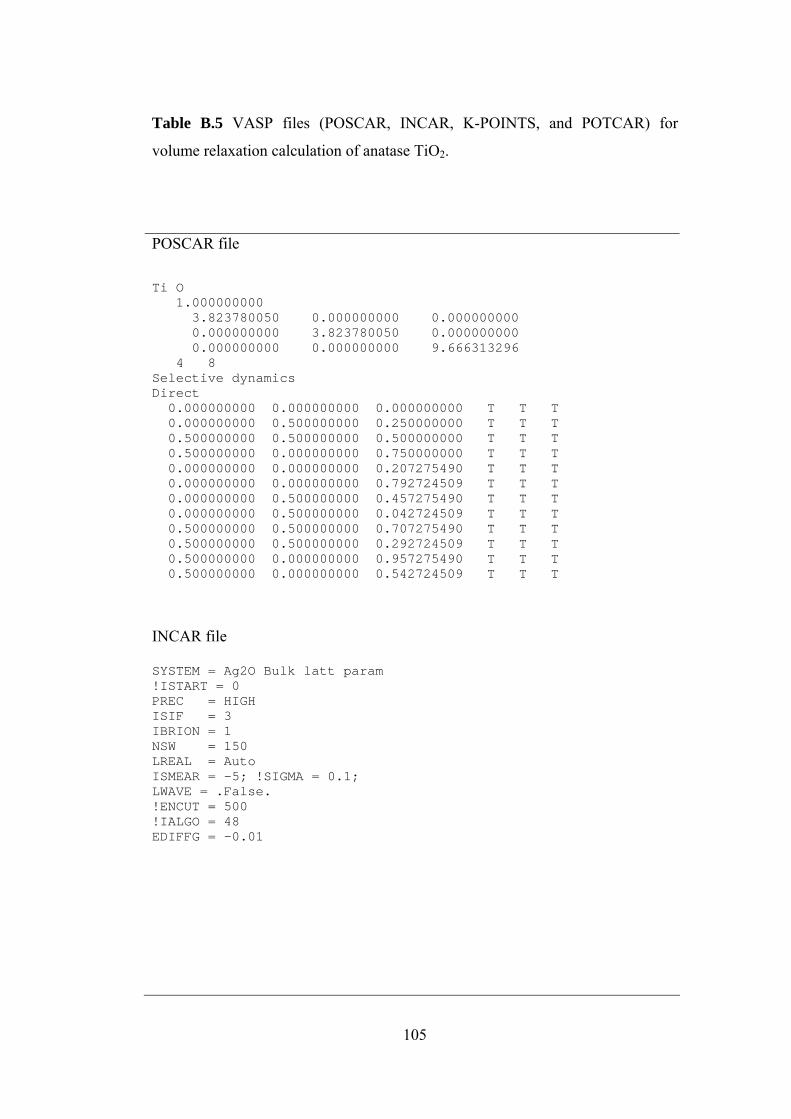
105

Table B.5 VASP files (POSCAR, INCAR, K-POINTS, and POTCAR) for

volume relaxation calculation of anatase TiO2.

POSCAR file

Ti O 1.000000000 3.823780050 0.000000000 0.000000000 0.000000000 3.823780050 0.000000000 0.000000000 0.000000000 9.666313296 4 8 Selective dynamics Direct 0.000000000 0.000000000 0.000000000 T T T 0.000000000 0.500000000 0.250000000 T T T 0.500000000 0.500000000 0.500000000 T T T 0.500000000 0.000000000 0.750000000 T T T 0.000000000 0.000000000 0.207275490 T T T 0.000000000 0.000000000 0.792724509 T T T 0.000000000 0.500000000 0.457275490 T T T 0.000000000 0.500000000 0.042724509 T T T 0.500000000 0.500000000 0.707275490 T T T 0.500000000 0.500000000 0.292724509 T T T 0.500000000 0.000000000 0.957275490 T T T 0.500000000 0.000000000 0.542724509 T T T INCAR file SYSTEM = Ag2O Bulk latt param !ISTART = 0 PREC = HIGH ISIF = 3 IBRION = 1 NSW = 150 LREAL = Auto ISMEAR = -5; !SIGMA = 0.1; LWAVE = .False. !ENCUT = 500 !IALGO = 48 EDIFFG = -0.01

106

Table B.5 (cont’d) K-POINTS file K-Points 0 Monkhorst Pack 15 15 15 0 0 0 POTCAR file PAW_GGA Ti 08Aug2001 4.00000000000000000 parameters from PSCTR are: VRHFIN =Ti: d3 s1 LEXCH = 91 EATOM = 95.1745 eV, 6.9951 Ry TITEL = PAW_GGA Ti 08Aug2001 LULTRA = F use ultrasoft PP ? IUNSCR = 1 unscreen: 0-lin 1-nonlin 2-no RPACOR = 2.200 partial core radius POMASS = 47.880; ZVAL = 4.000 mass and valenz RCORE = 2.800 outmost cutoff radius RWIGS = 2.500; RWIGS = 1.323 wigner-seitz radius (au A) ENMAX = 178.367; ENMIN = 133.775 eV RCLOC = 2.215 cutoff for local pot LCOR = T correct aug charges LPAW = T paw PP EAUG = 328.883 DEXC = -.021 RMAX = 3.452 core radius for proj-oper RAUG = 1.300 factor for augmentation sphere RDEP = 2.885 radius for radial grids QCUT = -3.621; QGAM = 7.241 optimization parameters “The following part in POTCAR file is cut in order to save place”

A QUANTUM CHEMICAL STUDY OF TITANIUM DIOXIDE SURFACES

Documents

Transcript of A QUANTUM CHEMICAL STUDY OF TITANIUM DIOXIDE SURFACES