1

User’s Guide

DipAnalyst 2.0 for Windows

Software for Kinematic Analysis of Rock Slopes

Developed by

Yonathan Admassu, Ph.D.

Engineering Geologist

E-mail: DipAnalyst 2.0@gmail.com Tel: 330 289 8226

Copyright © 2012

2

Welcome to DipAnalyst 2.0 for Windows

TERMS OF USE FOR DIPANALYST 2.0 1. The program described below refers to DipAnalyst 2.0.

2. This program is in trial version and is NOT for sale.

3. You may not extend the use of the program beyond the date allowed by the author without

permission.

4. You may use the program only on a single computer.

5. You may make one copy of the program for backup only in support of use on a single computer

and not use it on any other computer.

6. You may not use, copy, modify, or transfer the program, or any copy, in whole or part. You may

not engage in any activity to obtain the source code of the program.

7. You may not sell, sub-license, rent, or lease this program.

8. No responsibility is assumed by the author for any errors, mistakes in the program.

9. No responsibility is assumed by the author for any misrepresentations by a user that may occur

while using the program

10. No responsibility is assumed for any indirect, special, incidental or consequential damages arising

from use of the program.

3

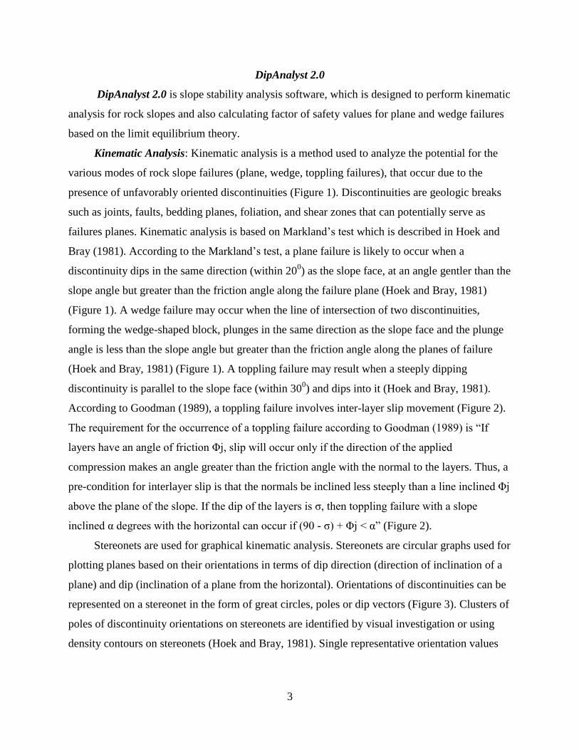
DipAnalyst 2.0

DipAnalyst 2.0 is slope stability analysis software, which is designed to perform kinematic

analysis for rock slopes and also calculating factor of safety values for plane and wedge failures

based on the limit equilibrium theory.

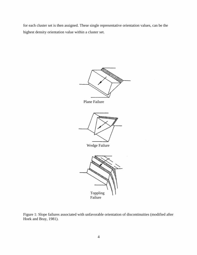
Kinematic Analysis: Kinematic analysis is a method used to analyze the potential for the

various modes of rock slope failures (plane, wedge, toppling failures), that occur due to the

presence of unfavorably oriented discontinuities (Figure 1). Discontinuities are geologic breaks

such as joints, faults, bedding planes, foliation, and shear zones that can potentially serve as

failures planes. Kinematic analysis is based on Markland’s test which is described in Hoek and

Bray (1981). According to the Markland’s test, a plane failure is likely to occur when a

discontinuity dips in the same direction (within 200) as the slope face, at an angle gentler than the

slope angle but greater than the friction angle along the failure plane (Hoek and Bray, 1981)

(Figure 1). A wedge failure may occur when the line of intersection of two discontinuities,

forming the wedge-shaped block, plunges in the same direction as the slope face and the plunge

angle is less than the slope angle but greater than the friction angle along the planes of failure

(Hoek and Bray, 1981) (Figure 1). A toppling failure may result when a steeply dipping

discontinuity is parallel to the slope face (within 300) and dips into it (Hoek and Bray, 1981).

According to Goodman (1989), a toppling failure involves inter-layer slip movement (Figure 2).

The requirement for the occurrence of a toppling failure according to Goodman (1989) is “If

layers have an angle of friction Φj, slip will occur only if the direction of the applied

compression makes an angle greater than the friction angle with the normal to the layers. Thus, a

pre-condition for interlayer slip is that the normals be inclined less steeply than a line inclined Φj

above the plane of the slope. If the dip of the layers is σ, then toppling failure with a slope

inclined α degrees with the horizontal can occur if (90 - σ) + Φj < α” (Figure 2).

Stereonets are used for graphical kinematic analysis. Stereonets are circular graphs used for

plotting planes based on their orientations in terms of dip direction (direction of inclination of a

plane) and dip (inclination of a plane from the horizontal). Orientations of discontinuities can be

represented on a stereonet in the form of great circles, poles or dip vectors (Figure 3). Clusters of

poles of discontinuity orientations on stereonets are identified by visual investigation or using

density contours on stereonets (Hoek and Bray, 1981). Single representative orientation values

4

for each cluster set is then assigned. These single representative orientation values, can be the

highest density orientation value within a cluster set.

Figure 1: Slope failures associated with unfavorable orientation of discontinuities (modified after

Hoek and Bray, 1981).

Plane Failure

Wedge Failure

Toppling

Failure

5

Figure 2: Kinematics of toppling failure (Goodman, 1989). α is slope angle, σ is dip of

discontinuity, Φj is the friction angle along discontinuity surfaces and N is the normal to

discontinuity planes. The condition for toppling is (90 - σ) + Φj < α.

Figure 3: Stereonet showing a great circle, a pole and dip vector representing a discontinuity with

a dip direction of 45 degrees E of N and dip of 45 degrees (figure created using RockPack).

90 - σ

Φj

N

σ

α

Great circle

(horizontal projection

of intersection of a plane with a lower

hemisphere of a

sphere)

Dip vector (orientation

of a point representing a line that has the

maximum inclination

on a plane)

Pole (orientation of a

point representing a

line that is perpendicular to a

plane)

6

Figure 4: a) stereonet showing 4 clusters of poles, b) density contoured poles for the poles shown

in (a). Contours spaced at every 1% pole density.

Alternatively, the mean dip direction/dip of cluster of poles is calculated as follows

(Borradaille, 2003) (Figure 4).

Mean dip direction = arctan (Y / X ) (1)

Mean Dip = arcsin ( z ) (2)

Where X = 1/R ∑ Li Y = 1/R ∑ Mi z = 1/R ∑ Ni

Li = cosIi cosDi, Mi = cosIi sin Di, Ni = sin Ii (3)

Where, Ii = individual dip direction, Di = individual dip

R2 = (∑ Li)

2 + (∑ Mi)

2 + (∑ Ni)

2 (4)

If a line survey or a drilled core is used to collect discontinuity data, some discontinuity

orientations can be over represented, if they have strike directions nearly perpendicular to the

scan line. Such sampling bias also affects the value of mean orientation values and Terzaghi’s

(1965) weight factors for each discontinuity data should be used. Based on Terzaghi (1965) and

Priest (1993) the probability that a certain discontinuity can be crossed by a certain scan line of a

certain trend and plunge can be estimated by:

Cluster of poles Highest density within a

cluster

7

cos = snsnsn sinsincoscos)cos( (5)

Where s = trend of scan line

n = trend of a normal line to a discontinuity

s = plunge of scan line

n = plunge of a normal line to a discontinuity

The weight (wi) assigned to a discontinuity plane based on the trend and plunge of a scan line is

given by:

wi=1/ cos (6)

Since the value of wi can be a large number, Priest(1993) suggests using a normalized

weight (wni), whose summation is the same as total number discontinuity count. wni is

calculated as follows:

wni = wi (N/Nw), (7)

Where N is the total number discontinuity data, and Nw is the summation of wi.

Equation (3) can now be re-written as:

Li = wni cosIi cosDi, Mi = wni cosIi sin Di, Ni = wni sin Ii (8)

If no bias exists, wni can be set to one.

Great circles for representative orientation values along with great circle for slope face

and the friction circle are plotted on the same stereonet to evaluate the potential for

discontinuity-orientation dependent failures (Figures 5,6,7) (Hoek and Bray, 1981). This

stereonet-based analysis is qualitative in nature and requires the presence of tight data clusters

for which a reasonable representative orientation value can be assigned. The chosen

representative value may or may not be a good representation for a cluster set depending on the

tightness of data within a cluster. Tight circular data is more uniform and has less variation

making representative values more meaningful than for cases where data shows a wide scatter.

Fisher’s K value is used to describe the tightness of a scatter (Fisher, 1953). It is calculated as

follows:

K = M – 1/M-|rn|, where M is no. of data within a cluster, and |rn| is the magnitude of

resultant vector for the cluster set (Fisher, 1953).

High K values indicate tightly clustered data, i.e. well-developed cluster set. If the cluster

set is tight, the representative values are more reliable and so is the stereonet-based kinematic

analysis. However, there are cases when a tight circular clustering of discontinuity orientations

8

does not exist. A different quantitative approach can be performed by DipAnalyst 2.0, which can

also be used for the stereonet-based method.

DipAnalyst 2.0 is an application software that is developed for stereonet-based analysis as

well as a new quantitative kinematic analysis. The quantitative kinematic analysis, instead of

relying on representative values, considers all discontinuities and their possible intersections to

calculate failure indices. Failure indices are calculated based on the ratio of the number of

discontinuities that cause plane failures or toppling failures or the number of intersection lines

that cause wedge failures to the total number of discontinuities or intersection lines. If

discontinuity data was collected along a scan line or drill core, some discontinuity orientations

will be overrepresented and other underrepresented. Therefore, instead of considering just the

number of discontinuities or possible intersections that cause failure, normalized weights are

recommended as they would remove the unwanted effects of over represented discontinuity data.

DipAnalyst 2.0 compares every dip direction/dip value with slope angle and friction angle to

evaluate its potential to cause plane or toppling failure. It also calculates all potential intersection

line plunge direction and amount for wedge failure potential.

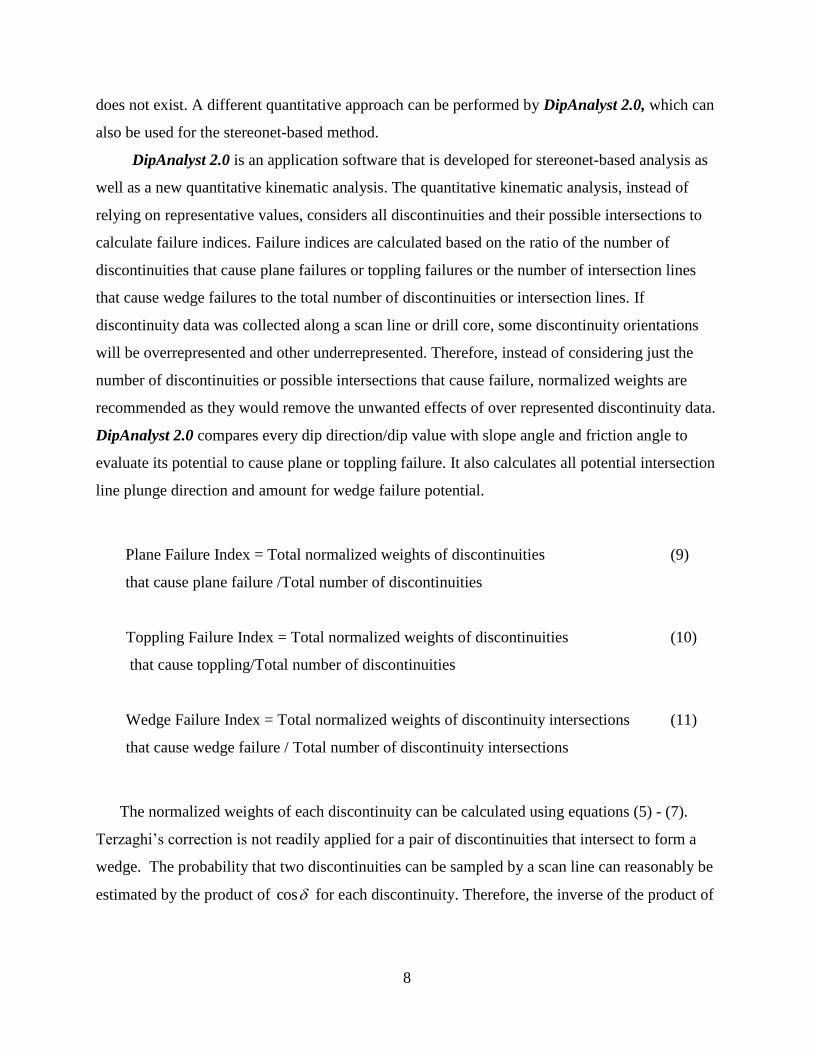
Plane Failure Index = Total normalized weights of discontinuities (9)

that cause plane failure /Total number of discontinuities

Toppling Failure Index = Total normalized weights of discontinuities (10)

that cause toppling/Total number of discontinuities

Wedge Failure Index = Total normalized weights of discontinuity intersections (11)

that cause wedge failure / Total number of discontinuity intersections

The normalized weights of each discontinuity can be calculated using equations (5) - (7).

Terzaghi’s correction is not readily applied for a pair of discontinuities that intersect to form a

wedge. The probability that two discontinuities can be sampled by a scan line can reasonably be

estimated by the product of cos for each discontinuity. Therefore, the inverse of the product of

9

cos 1 for discontinuity 1 and cos 2 for discontinuity 2, can be used as the weight factor for

each intersection.

The weight factor for each intersection can be calculated as follows:

wi = 1/( cos 1 cos 2) (12)

The normalized weight factor wni can be calculated using equation (7). The sum of wni is equal

to the total number of discontinuity intersections. One can set wni values to unity if there is no

bias during data collection.

Failure indices are therefore the sum of normalized weights of discontinuities that have the

potential to fail, divided by the total number of discontinuities. A higher index value for a given

type of failure indicates a greater chance for that type of failure to occur. DipAnalyst 2.0 also

allows a simple sensitivity analysis to evaluate the change of failure indices with changing

friction angles, slope angles, and slope azimuths. The quantitative approach for kinematic

analysis can be easily interpreted by professionals who are not familiar with the use of

stereonets.

Figure 5: Stereographic plot showing requirements for a plane failure (Hoek and Bray, 1981,

Watts 2003). If the dip vector (middle point of the great circle) of the great circle representing a

discontinuity set falls within the shaded area (area where the friction angle is higher than slope

angle), the potential for a plane failure exists (figure created using RockPack).

Representative dip vector for a discontinuity

set

Representative pole for a discontinuity set

Shaded critical zone

10

Figure 6: Stereographic plot showing requirements for a wedge failure (Hoek and Bray, 1981,

Watts 2003). If the intersection of two great circles representing discontinuities falls within the

shaded area (area where the friction angle is higher than slope angle), the potential for a wedge

failure exists (figure created using RockPack software).

Figure 7: Stereographic plot showing requirements for a toppling failure (Goodman, 1989, Watts

2003). The potential for a toppling failure exists if dip vector (middle point of the great circle)

falls in the triangular shaded zone (figure created using RockPack software).

Great circle for discontinuity cluster

set 2

Great circle for discontinuity

cluster set 1

Shaded critical zone

Triangular critical zone for

toppling failure

Representative dip

vector for a

discontinuity set

Representative pole

for a discontinuity set

Line of intersection between the

representative orientations of the

two discontinuity sets

11

Factor of Safety Calculations: Limit equilibrium analysis is used to calculate the factor

of safety (F.S.) of a slope against failure once the kinematic analysis indicates the potential for

failure. Factor of safety is the ratio of the resisting forces (shear strength) that tend to oppose the

slope movement to the driving forces (shear stress) that tend to cause the movement along a

plane of discontinuity. The equation for F.S. is:

F.S. = (c + tan )/ (13)

Where: F.S. = factor of safety

c = cohesion

= angle of internal friction

= normal stress on slip surface

= shear stress

According to the limit equilibrium approach, a factor of safety value equal to 1 represents

limiting condition, a value greater than 1 represents a stable slope, and a value less than 1

indicates an unstable slope. The desired value of factor of safety depends upon the importance of

the slope and the consequences of failure. For heavily travelled roads, slopes are usually

designed to have a factor of safety equal to or greater than 1.3 under saturated conditions,

maximum loads, and worst expected geological conditions (Canadian Geotechnical Society,

1992; Wyllie and Mah, 2004). The equations derived for both plane and wedge failure, consider

weight of the sliding block, cohesion along plane of discontinuity, effect of water present along

planes of discontinuity and tension applied from a rock bolt. Although the equations for factor of

safety calculations of plane and wedge failures are based on Equation (13), they vary due to

differences in the shape of the sliding block for the case of plane vs. wedge failures. The

methods for calculating the factor of safety for plane and wedge failures with corresponding

12

equations to determine the resisting and driving forces, including the effect of water pressure

along discontinuities and application of a rock bolt are given in Hoek and Bray (1981) and

Wyllie and Mah (2004).

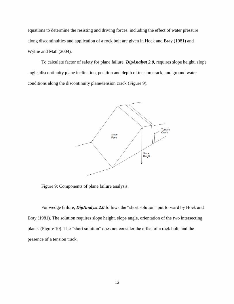
To calculate factor of safety for plane failure, DipAnalyst 2.0, requires slope height, slope

angle, discontinuity plane inclination, position and depth of tension crack, and ground water

conditions along the discontinuity plane/tension crack (Figure 9).

Figure 9: Components of plane failure analysis.

For wedge failure, DipAnalyst 2.0 follows the “short solution” put forward by Hoek and

Bray (1981). The solution requires slope height, slope angle, orientation of the two intersecting

planes (Figure 10). The “short solution” does not consider the effect of a rock bolt, and the

presence of a tension track.

13

Figure 10: Components of wedge failure analysis.

14

Using DipAnalyst 2.0

Entering, Opening and Saving Data

New data can be entered directly onto the dip direction and dip columns or can be imported

from a .csv file, where the first column contains dip direction, the second column contains dip

values and the third contains symbol codes. .csv files can be created with Microsoft excel. Dip

direction and dip data can be saved as .csv file. Slope azimuth, slope angle, and friction angle

need to be entered. To correct for bias arising from scan line orientation, scan line information

should be entered in this window.

Refresh

The ‘Refresh’ tool calculates the azimuths and plunges of all possible lines of intersection

between all possibly intersecting discontinuity planes. Once executed, the other icons will be

functional. Every time a new discontinuity data set is entered or an opened data is modified, the

15

‘Refresh’ should be run. To consider normalized weights based on scan line trend and plunge,

the “use weighted values” checkbox should be checked in the data entry window.

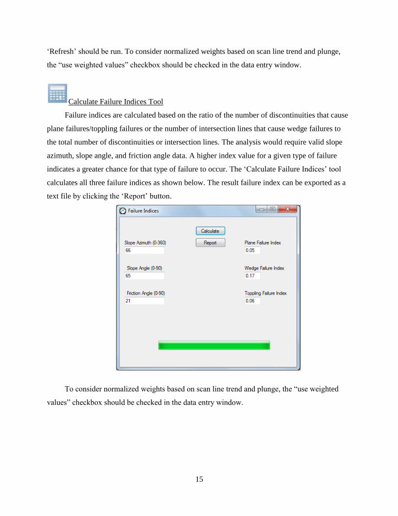
Calculate Failure Indices Tool

Failure indices are calculated based on the ratio of the number of discontinuities that cause

plane failures/toppling failures or the number of intersection lines that cause wedge failures to

the total number of discontinuities or intersection lines. The analysis would require valid slope

azimuth, slope angle, and friction angle data. A higher index value for a given type of failure

indicates a greater chance for that type of failure to occur. The ‘Calculate Failure Indices’ tool

calculates all three failure indices as shown below. The result failure index can be exported as a

text file by clicking the ‘Report’ button.

To consider normalized weights based on scan line trend and plunge, the “use weighted

values” checkbox should be checked in the data entry window.

16

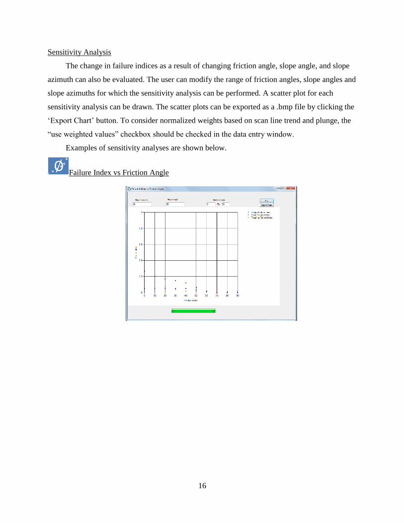
Sensitivity Analysis

The change in failure indices as a result of changing friction angle, slope angle, and slope

azimuth can also be evaluated. The user can modify the range of friction angles, slope angles and

slope azimuths for which the sensitivity analysis can be performed. A scatter plot for each

sensitivity analysis can be drawn. The scatter plots can be exported as a .bmp file by clicking the

‘Export Chart’ button. To consider normalized weights based on scan line trend and plunge, the

“use weighted values” checkbox should be checked in the data entry window.

Examples of sensitivity analyses are shown below.

Failure Index vs Friction Angle

17

Failure Index vs Slope Angle

Failure Index vs Slope Azimuth

Stereonet

The ‘Stereonet’ tool opens the ‘Stereonet’ window. Poles, dip vectors and plunge of all

possible intersection lines can be plotted on the stereonet by clicking ‘Draw’ button. Based

18

the symbol codes entered in the data entry, dip vectors and poles may be represented by

different symbols.

The ‘stereonet’ tool also allows stereonet-based kinematic analysis by checking the ‘Dip

Vectors, Great Circles, Friction Angle’ radio button and clicking ‘Draw’. Plane and toppling

failure indices are also provided on the stereonet with dip vectors.

The stereonet-based kinematic analysis for wedge failure can be performed based on

plunges of all possible intersection lines as shown below.

Slope face

Toppling zone satisfying

Goodman’s (1989)

criteria

Dip vectors

within these

boundary lines

are within 200 to

the slope face.

19

Wedge failure indices are provided at the corner of the stereonet. To consider normalized

weights based on scan line trend and plunge for indices calculation, the “use weighted values”

checkbox should be checked stereonet window.

Selection of Discontinuity Sets

Cluster of discontinuities can be visually identified from pole plot of discontinuities.

Selection can be done by left clicking at the upper left corner of the cluster set and holding down

the mouse until reaching the lower right corner of the cluster set. The selected poles will be

highlighted and the boundary around the selected set will be visible. The mean dip direction, dip,

percentage of selected discontinuities, and Fisher’s K value can then be added into discontinuity

set table by clicking the ‘Add Selected Set’ button. To consider weighted values, the “use

weighted values” checkbox should be clicked in the stereonet window. Clicking ‘Add Selected

Set’ would also open the ‘Failure Potential’ window which contains the discontinuity set table.

20

Evaluating Discontinuity Sets

The selected joint sets can be evaluated by clicking the ‘Evaluate Discontinuity Sets’

button. The result is a text report of the mean dip direction, mean dip, percentage of selected

discontinuities, and Fisher’s K values. It will also report on which discontinuity sets would cause

plane and toppling failures as well as which intersecting discontinuity cluster sets will cause

wedge failures.

21

Great circles representing discontinuity sets, slope face and the friction circle will be drawn

by clicking ‘Plot Sets on Stereonet’ button.

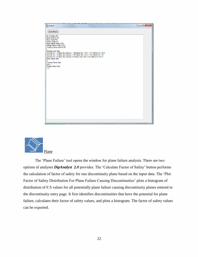
Report

The ‘Report’ tool will open a window with a text box showing the result of failure indices

calculation performed within the ‘Failure Indices’ window and discontinuity set evaluation

within the ‘Failure Potential’ window. The ‘Report’ button should be clicked in the ‘Failure

Indices’ window and/or ‘Failure Potential’ window for the ‘Report’ tool to record a report.

22

Plane

The ‘Plane Failure’ tool opens the window for plane failure analysis. There are two

options of analyses DipAnalyst 2.0 provides. The ‘Calculate Factor of Safety’ button performs

the calculation of factor of safety for one discontinuity plane based on the input data. The ‘Plot

Factor of Safety Distribution For Plane Failure Causing Discontinuities’ plots a histogram of

distribution of F.S values for all potentially plane failure causing discontinuity planes entered in

the discontinuity entry page. It first identifies discontinuities that have the potential for plane

failure, calculates their factor of safety values, and plots a histogram. The factor of safety values

can be exported.

23

Wedge

The ‘Wedge Failure’ tool opens the wedge failure analysis window. Similar to

plane failure analysis, DipAnalyst 2.0 can calculate factor of safety for a single wedge defined by

a pair of discontinuities as well as plot distribution of factor of safety values for all possible

intersecting discontinuities that potentially can lead to wedge failures. The factor of safety values

can be exported.

24

REFERENCES

Borradaile, G., 2003. Statistics of Earth Science Data, Springer, New York, USA, 351pp.

Canadian Geotechnical Society, 1992, Canadian Foundation Engineering Manual,

BiTech Publishers Ltd., Vancouver, Canada.

Fisher, R.,A., 1953. Dispersion on a sphere. In: Proceedings of the Royal society of

London, A217, pp.295-305.

Goodman, R. E., 1989. Introduction to Rock Mechanics, John Wiley & Sons, New York,

USA, 562pp.

Hoek, E. and Bray, J. W., 1981. Rock Slope Engineering, 3rd edn., The Institute of

Mining and Metallurgy, London, England, 358 pp.

Priest, S.D, 1993. Discontinuity Analysis for Rock Engineering, Chapman & Hall Ltd.,

London, UK, 473pp.

Terzaghi, R.D., 1965. Sources of error in joint surveys. Geotechnique 15, 287-304.

Watts, C.F., Gilliam, D.R., Hrovatic, M.D., and, Hong, H., 2003. User’s Manual-ROCKPACK III

for Windows, C.F.Watts and Associates, Radford, VA, USA, 33 pp.

Wyllie, D. C. and Mah, C. W., 2004, Rock slope Engineering: 4th

Edition, Spon Press,

London and New York, 432p.