HAL Id: hal-01551476https://hal.archives-ouvertes.fr/hal-01551476

Submitted on 30 Jun 2017

HAL is a multi-disciplinary open accessarchive for the deposit and dissemination of sci-entific research documents, whether they are pub-lished or not. The documents may come fromteaching and research institutions in France orabroad, or from public or private research centers.

L’archive ouverte pluridisciplinaire HAL, estdestinée au dépôt et à la diffusion de documentsscientifiques de niveau recherche, publiés ou non,émanant des établissements d’enseignement et derecherche français ou étrangers, des laboratoirespublics ou privés.

A Quadratic Model and A Heuristic for Sizing anHybrid Renewable Energy System

Serigne Gueye, Rachid Belfkira, Georges Barakat, Adnan Yassine

To cite this version:Serigne Gueye, Rachid Belfkira, Georges Barakat, Adnan Yassine. A Quadratic Model and A Heuristicfor Sizing an Hybrid Renewable Energy System. Operational Research Practice in Africa (ORPA),2010, Dakar, Senegal. �hal-01551476�

Technical Report LMAH, 2009

A Quadratic Model and A Heuristic for Sizing an Hybrid

Renewable Energy System.

Serigne Gueye · Rachid Belfkira ·

Georges Barakat · Adnan Yassine

December 29, 2009

Abstract An Hybrid Renewable Energy System (HRES) may be defined as

a system in which various renewable energy components (solar panels, wind

turbines,...,batteries) are interconnected in such a way to satisfy, at any time,

a demand of electrical energy. Since electrical power supplied by each compo-

nent (taking independently) depends on different environment conditions (sun,

wind), and since the demand fluctuates, the objective of such system is to be

able to produce energy at any time by optimally exploiting favourable weather

Serigne Gueye · Adnan Yassine

Universite du Havre, Laboratoire de Mathematiques Appliquees du Havre (LMAH), BP 540,

76058 Le Havre cedex, France.

E-mail: serigne.gueye,adnan.yassine@univ-lehavre.fr

Rachid Belfkira · Georges Barakat

Universite du Havre, Groupe de Recherche en Electronique et Automatique du Havre

(GREAH), BP 540, 76058 Le Havre cedex, France.

E-mail: rachid.belfkira,georges.barakat@univ-lehavre.fr

2

conditions for each component, and to stock available energy (for latter use

in non favourable conditions) of surproduction periods. The induced problem

is to compute the optimal number of each component, minimizing installation

and maintenance costs. We propose an integer quadratic programming model

to solve this problem. The model is linearized and solved with a heuristic

scheme. Numerical results, based on data obtained on a site in Dakar (Sene-

gal) in which the system has to be installed, are provided.

Keywords 0-1 Quadratic Programming, Heuristic, Linearization, Renewable

Energy system.

1 Introduction

Renewable energy is energy generated from natural resources such as sunlight,

wind, rain, tides, which are naturally replenished. The environmental prob-

lems, high oil prices and increasing government support, are driving increasing

renewable-energy commercialization. The industry is currently growing more

and more. From the end of 2004 to the end of 2008, solar photovoltaic (PV)

capacity increased sixfold to more than 16 gigawatts (GW), wind power ca-

pacity increased 250 percent to 121 GW, and total power capacity from new

renewables increased 75 percent to 280 GW. The renewable energy technolo-

gies are non-polluting but in the same time suffer to at least two ”critics”.

It is well known that the electrical power generation from the renewable energy

technology is site-dependent and intermittent. The power generated depends

3

on the environment conditions, which fluctuate randomly and impact con-

siderably the power generation. However, some of them have complementary

profiles. This is specially the case for solar and wind energy. For instance, in

summer significant solar radiations may be expected whereas in winter wind

speed is higher. In a geographical point of view, the locations of a country (or

a region) may also have complementary potential in the sense that some loca-

tions may be more suitable for a kind of renewable energy than some others.

For example, the north-west european coast benefit to high wind exposition

while in the south solar radiations are higher. Hence, one may imagine systems

exploiting as best as possible weather conditions of any seasons, or potential

of regions (or locations), in such a way to deliver at any time required elec-

trical power. A part of this kind of system limited to individual uses (not

at a scale of regional or country production) have been imagined by GREAH

Researchers (Groupe de Recherche en Electronique et Automatique du Havre).

The expensive installation and maintenance costs of renewable energy sys-

tems, in comparison to other energy sources (gas, oil,...), is also a critical

point. Wind and solar power costs are currently higher than gas or oil energy

sources but the trend is going down with economies of scale and better mate-

rials. Thus, when implementing any renewable energy technology, one has to

analyze carefully the problem of optimizing induced costs.

The hybrid system proposed by Belfkira et al [1] may be summarized as in the

4

figure 1. Very schematically, it may be viewed as a network where the sources

are the wind turbines and solar panels and the destination is the customers.

The energy flow fulfilled by the sources is summed up on a so called ”bus”.

When the customer demands are lower to the energy supplied the surplus

are stored in batteries. In the case of bad weather conditions, the demand

may exceed the offer of the sources, hence the batteries are used if possible.

Many additional power equipments (rectifier, chopper,...) are necessary to im-

plement in practice this system. The explanations of such equipments is out

of the scope of this paper. Shortly, these equipments are used to convert the

electrical power from a given form to another (i.e Alternative Current (AC)

to Direct Current (DC) and vice versa).

Each material of this sytem is expensive in terms of installation and main-

tenance costs. Thus, we seek to find the optimal numbers of solar panels, wind

turbines and batteries needed to satisfy the demand of electrical energy at

any time of the year. These optimal numbers correspond to the minimal ac-

quisition, installation and maintenance costs of the system. The demand of

electrical energy and the amount of enegy that may be produced by the dif-

ferent sources are in practice difficult to know accurately since it depends on

customer consumption profiles, meteorologic conditions during a year, etc. To

evaluate this demand two approaches may be used : stochastic and determinis-

tic. In the stochastic approach the demand and power of the renewable energy

sources over the time are modelized as stochastic variables, then a stochastic

5

Fig. 1 HRES

programming model has to be solved. In the deterministic case, an observation

period of length T is considered, for instance 6 significant months of the year.

This period is discretized (i.e t = 0, ..., T ). Then at any time t, the demand

is evaluated by a constant giving the average consumption. Observations are

also done in this period on solar radiations, temperature, wind speed. These

data are then used to evaluate at each time t the electrical power generated

by solar panels and wind turbines of different types. This paper is concerned

with the deterministic approach.

In section 2, we introduce data notations. In section 3, we detail the quadratic

model proposed to find the optimal size of the renewable energy system taking

into account deterministic informations. The model has been applied to size a

renewable energy system in a site located at the Cheikh Anta Diop University

at Dakar (Senegal). The observation period considered in this site is 6 months

with a discretization of 1 hour. This small step of discretization induced a

very large scale mathematical program, impossible to solve optimally in our

6

Fig. 2 Supply Chain

computing environment. A heuristic is then proposed in section 4. The numer-

ical results are provided in section 5. Finally conclusion and perspectives are

drawn in section 6.

2 Renewable Energy Supply Chain

Providing electrical energy corresponding to customer demands may be rep-

resented as a supply chain starting from the renewable energy sources and

ending at the final consumers as shown in figure 2. At any time of the year

(from January to December) and in any weather conditions we want to im-

plement an Hybrid Renewable Energy System (HRES for short) giving the

required quantity of energy. The sizing decision problem is located precisely in

the link ”HRES System” of this logistic chain. For this decision, informations

about the links at the left (Site) and at the right (Demand) of the HRES

system is necessary at any time. These informations are obtained by obser-

vations in a given period of the year. A period of size T (6 to 12 months) is

chosen and discretized , i.e t = 0, 1, , 2, ..., T . At any time t, some measures

7

are performed related to site and demand properties : solar radiations, tem-

perature and wind speed. The informations about the customers consist on

an evaluation of the demand at time t. All of these data are supposed to be

fixed scalar. With these data and additional informations about the physi-

cal properties of the renewable energy components, it is possible to compute

at any time t the power fulfilled by each component and the customer demand.

We notice dt the demand at time t. Let us consider that different types

i = 1, ..., I (resp. j = 1, ..., J) of solar panels (resp. wind turbines) exist.

The (known) electrical power provided by a solar panel (resp. wind turbine of

type j) of type i at time t is noticed Pit (resp. Wjt). Pit and Wjt values are

given by equations depending on material and site properties.

Given the demand dt and powers Pit and Wjt, our purpose is to size the

HRES System in such a way to minimize the installation and maintenance

costs with respect to the demand and the batteries life cycle. The next section

deals with the associated optimization model.

3 Model

We subdivide the model presentation in subsections corresponding to the dif-

ferent parts of any mathematical program : Decision variables, Objective Func-

tion, Constraints.

8

3.1 Decision Variables

Decisions that we have to take deal with the optimal numbers of solar pan-

els, wind turbines and batteries. In order to understand the meaning of the

variables, we briefly show below how the renewable energy components of the

system are organized. The solar panels, of type i, are interconnected in se-

ries and in parallel in a matrix structure called ”PV array” where PV stands

for photovoltaic (see figure 3 below). Vertical connexions are called ”strings”.

Fig. 3 PV array

Strings are connected in parallel, providing a PV Array. Let us notice vsi (resp.

vpi ) the number of solar panels connected in series (resp. parallel). vsi do not

depends, in practice, on site or demand properties but only on system proper-

ties. Using electrical engineering theory, vsi may be computed accurately. This

is a constant. At the opposed, the suitable value of vpi depends on the envi-

ronment and on the demand. Hence, vpi is a decision variable. Let us remark

that each type corresponds to a PV array. Since the number (I) of solar types

is fixed, the number of PV array is upper bounded by I. Our decision is thus

9

to find how many strings to install for each PV array type. vpi = 0 means that

the PV array i will not be implemented.

Batteries are organized as solar panels. Similar picture as above may be also

used for battery array by replacing the solar panels by batteries. We notice

ysk (resp. ypk) the number of batteries of type k connected in series (resp. in

parallel). As for solar panels, ysk is known and ypk is a decision variable. The

HRES system is supposed to use battery panels when the renewable energy

quantity is unsufficient, and to store electrical energy in batteries when the

offer exceeds the demand. The set of all batteries of any type is called the bat-

tery bank, and Yt stands for the total amount of electrical power available in

this bank. Since this bank may be used to store or to keep energy, the values of

Yt should reflect these two alternatives. By convention, a positive value of Yt

means that the bank is in charging process (energy storage) while a negative

value stands for discharging process.

A wind turbine is composed of two parts : a tower and the turbine composed

of rotor shaft, and electrical generator at the top of the tower. The number of

wind turbines of type j to install will be noticed tj .

The variables vpi , tj , ypk are integers while Yt is continuous. These integer

variables will be bounded respectively by maximal number of solar strings of

type i in parallel (vpi ), maximal number of wind turbines of type j (tj) and

10

maximal number of battery strings of type k in parallel (ypk).

i.e 0 ≤ vpi ≤ vpi i = 1, ..., I

0 ≤ ypk ≤ ypk k = 1, ...,K

0 ≤ tj ≤ tj j = 1, ..., J

3.2 Objective Function

For each component (solar panels, batteries and wind turbines), three costs

have been considered : the acquisition cost (noticed 1), the installation cost

(noticed 2) and the annual maintenance cost (noticed 3). We notice c1i (resp.

c2i , c3i ) the acquisition (resp. installation, maintenance) cost of a solar panel

of type i. We seek to optimize maintenance cost over a period of 20 years

generally admitted as the usual lifespan of solar panels and batteries. Hence,

the total cost of a solar panel of type i is

ci = c1i + c2i + 20c3i , i = 1, 2, ..., I.

Let b1k (resp. b2k, b3k) be the acquisition (resp. installation, maintenance) cost

of one battery of type k. At the opposed of solar panels, over the period

of 20 years, a battery will be changed rk times while solar panels are only

maintained. rk is fixed. The total cost of a battery of type k is then :

bk = b1k + b2k + (20− rk)b3k + rk(b

1k + b2k) , k = 1, 2, ...,K.

For explanation, battery is bought (b1k) and installed (b2k). When a battery is

11

changed no maintenance cost have to be considered but acquisition and in-

stallation (b1k + b2k). Thus the number of time that maintenance is performed

corresponds to 20− rk and the corresponding maintenance cost is (20− rk)b3k.

Some costs are associated to each part of a wind turbine. We notice w1j , w

2j ,

w3j the acquisition, installation and maintenance costs of a turbine of type j,

and h1j , h

2j , h

3j the acquisition, installation and maintenance costs of a tower

of type j. The resulting total cost is :

wj = w1j + w2

j + 20w3j + h1

j + h2j + 20h3

j .

With these notations, the total cost of the renewable energy components, plus

the batteries cost is

I∑i=1

civsi v

pi +

K∑k=1

bkysky

pk +

J∑j=1

wjtj .

This is the objective function that we have to minimize. Notice that the func-

tion is linear since vsi and ysk are known. vsi vpi is the total number of solar panels

of type i for the PV array of type i. Since each one cost ci, the total cost of

a panel of type i is civsi v

pi . The expression of the batteries cost is obtained

similarly.

3.3 Constraints

Two kind of constraints have been formulated : the demand constraints and

material constraints on batteries.

12

3.3.1 Demand constraints

At any time t, the total amount of energy produced must be greater or equal

to the demand dt. Since Pit is the power of a solar panel of type i at time t,

and Wjt the power of a wind turbine of type j at time t, then the total power

of solar panels and wind turbines is :

Et =

I∑i=1

Pitvsi v

pi +

J∑j=1

Wjttj , t = 0, 1, ..., T.

It follows that Et−Yt is the total energy fulfilled by renewable energy sources

and battery panels. This total energy must always fit the demand. The demand

constraints are then

Et − Yt ≥ dt , t = 0, 1, ..., T. (1)

3.3.2 Battery constraints

The total amount of energy in the battery bank is called the ”state of charge”

of the battery bank at time t and is noticed ut. For safety reasons and maximal

capacity of batteries, ut is bounded by known mimimal and maximal values u

and u.

u ≤ ut ≤ u , t = 0, 1, ..., T. (2)

If usk is the maximal capacity of a battery string of known size ysk then the

maximal capacity of a battery array with ypk strings of size ysk is ypkusk. It follows

that

u =K∑

k=1

ypkusk. (3)

13

u is a minimal value under which the battery must no be discharged to avoid

serious damages. Its value is obtained as follows :

u = (1−DoD)u, (4)

where DoD is calling the Depth of Decharge. DoD is a material property

provided by the battery manufacturer and giving the authorized discharging

percentage from the maximal capacity.

ut (t = 0, 1, ..., T ) is a serie expressed as follows :

u0 = u

ut+1 = ut +Yt

β η , if Yt ≥ 0 (charging process)

ut+1 = ut +Yt

β , if Yt < 0 (discharging process)

where η ∈ [0, 1] and β ≥ 0 are two physical properties expressing the per-

formance of the battery, and the HRES bus voltage.

To modelize the two possible values for ut+1, binary variables λt have been

introduced. Let

λt =

1 in the charging process

0 in the discharging process

With these variables, we have :

ut+1 = ut +Yt

β[ηλt + (1− λt)]

14

It follows (by reccurence) that

ut+1 = u+

t∑l=1

Yl

β[ηλl + (1− λl)] , t = 0, 1, ..., T. (5)

Thus, from inequations ( 2), and equations ( 3), ( 4) and ( 5), we deduce that

−DoD

K∑k=1

ypkusk ≤

t−1∑l=1

Yl

β[ηλl + (1− λl)] ≤ 0 , t = 1, 2, ..., T. (6)

In addition, we also have to link variables λt with Yt signs. When λt = 1

(resp. λt = 0) we are in charging (resp. discharging) process, so Yt must be

non negative (non positive). The resulting inequations are :

(1− λt)Y ≤ Yt ≤ λtY , 0 ≤ t ≤ T, (7)

where Y (resp. Y ) is the maximal (resp. minimal) possible total capacity in

the battery bank. Y and Y are computed using the upper bounds on variables

ypk. Y is the maximal capacity of the battery bank obtained by taking for each

type k the maximal value ypk,

i.e. Y =

K∑k=1

ypkuskβ,

and Y = −Y .

3.4 Final Formulation

With the subsections above the complete formulation for the optimal sizing

may be written. We have :

15

MODEL(T ) : MinI∑

i=1

civsi v

pi +

K∑k=1

bkysky

pk +

J∑j=1

wjtj

s-t ( 1)I∑

i=1

Pitvsi v

pi +

J∑j=1

Wjttj − Yt ≥ dt, 0 ≤ t ≤ T

( 6) −DoDK∑

k=1

ypkusk ≤

t−1∑l=1

Yl

β [ηλl + (1− λl)] ≤ 0, 1 ≤ t ≤ T

( 7) (1− λt)Y ≤ Yt ≤ λtY , 0 ≤ t ≤ T

0 ≤ vpi ≤ vpi i = 1, ..., I

0 ≤ ypk ≤ ypk k = 1, ...,K

0 ≤ tj ≤ tj j = 1, ..., J

4 Resolution

Following the formulation sections, we are interested here in the resolution

scheme of MODEL(T ). As a preliminary, let us first introduce some general

remarks on the problem. The objective function of the problem is linear, and

except the constraints (6) all others constraints are also linear. Depending on

the value of T the resulting formulation may be very large. In our numerical

experimentations, in section 5, T is equal to 4343 (6 months) and there are

two types of each renewable energy components. As a consequence, there are

:

16

– T + 1 binary variables λt = 4344

– T + 1 continuous variables Yt = 4344

– I = 2 : 2 types of solar panels.

– J = 2 : 2 types fo wind turbines.

– K = 2 : 2 types of batteries.

Hence, the total number of variables is 8694 variables in which 4350 are inte-

gers. We also have :

– T + 1 constraints (1) = 4344.

– 2 ∗ (T + 1) constraints (6) = 8686.

– 2 ∗ (T + 1) constraints (7) = 8688.

The total number of contraints is 21718. It follows, from this value of T , a

very large scale integer non linear mathematical program. Both for this huge

size and limited machine capacity, it has been chosen to solve this problem by

a heuristic. The resolution method is detailed in the sequel.

4.1 Heuristic

Our heuristic may be classified in referent domain optimization methods (see

Glover and Laguna [4]). The idea is quite simple. Solving exactly MODEL(T )

for little value of T is possible since the resulting formulation is also of little

17

size. Thus, even if we cannot solved MODEL(T ) for big value of T (such

as 4343), one may choose a lower value (says T′= 4344

2 = 2172), then solve

MODEL(T′ − 1), fixed all variables λt, Yt for t = 0, 1, ..., T

′ − 1 to their op-

timal values in MODEL(T′ − 1), and finally solved MODEL(2 ∗ T ′ − 1). In

doing so, at each of the two iterations, the number of variables λt and Yt of

the resulting problems are always divided by two.

Our heuristic is a sophistication of this idea in which any value for T′(not

necessarily T2 ) may be chosen and where the variables fixed at each iteration

are only binary variables λt. We choose to fix only variables λt because at

each iteration the optimal solution is obtained using a standard linearization

of the quadratically constrained problem MODEL(T ). In the resulting linear

formulation, the ”difficult” variables are not the continuous one’s (Yt) but the

binary one’s. The general scheme of our heuristic is summarized in figure 4.

Let T be the size of the observation period. Since T is currently too large, we

Fig. 4 Heuristic Scheme

take a much more lower period T′. T is then subdivided in b T

T ′ c subperiods

18

of size T′as shown in the figure. At the first iteration, MODEL(T

′ − 1) is

solved optimally. Then binary variables, {λt}t=0,1,..,T ′−1 are fixed (definitely)

to their optimal values. At the second iteration MODEL(2T′ − 1) is solved

and {λt}t=T ′+1,1,..,2T ′+1 are fixed, etc. The corresponding algorithm is the

following :

HEURISTIC

• T = 6 months of 1 hour step i.e 4343

• T′= value to be fixed (T

′<< T).

• newStart = 0

• newT = T′

While newT ≤ T

• Solve optimally MODEL(newT-1),

• Let λ∗B be optimal values of variables λB

• for t = newStart to newT-1

• λB(t) = λ∗B(t)

• newStart = newStart + T′

• newT = newT + T′

19

end While

Let Tk = kT′(0 ≤ k ≤ q) where q is the ratio of the division of T by T

′

i.e T = T′q + r with 0 ≤ r < q

Let also Tq+1 = T′q + r = T . T1, T2,...,Tq+1 are the discretization of [0, T ].

Let us consider two indices, i < j, of the set {1, 2, ..., q + 1}. We notice

(vp, yp, t, λ, Y ) a solution of MODEL(Tj) where : vp = (vp1 , vp2 , ..., v

pI ) ∈ NI ,

yp = (yp1 , vp2 , ..., v

pK) ∈ NK , t = (t1, t2, ..., tJ) ∈ NJ , λ = (λ0, λ2, ..., λTj ) ∈

{0, 1}Tj , and Y = (λ0, λ2, ..., λTi) ∈ RTj .

It can be ssen that by projecting λ (resp. Y ) on {0, 1}Ti (resp. RTi), the re-

sulting point (vp, yp, t, λ∗, Y ∗), where λ∗ (resp. Y ∗) are the restrictions of λ

on the space {0, 1}Ti (resp. RTi), remains feasible for MODEL(Ti). Thus we

have the following property.

Property 1 For any mathematical program (P ) let V (P ) denotes its optimal

value. We have V (MODEL(Ti)) ≤ V (MODEL(Tj)) ∀ 1 ≤ i ≤ j ≤ q + 1 2

It follows that since V (MODEL(T1)) ≤ V (MODEL(T2)) ≤ .... ≤ V (MODEL(T )),

V (MODEL(T1)) is a lower bound of the optimal value of MODEL(T ) that

may be used to evaluate the quality of the solution of the heuristic. It corre-

sponds, in our heuristic, to the optimal value computed at the first iteration of

the while loop. In the subsequent iterations, the objective values found cannot

be used as lower bounds since some variables λ has been fixed. Obviously,

notice that greater is the value T′and better is this lower bound. In our nu-

20

merical experiments (see section 5) this lower bound has been computed for

increasing value of T′.

4.2 Solving optimally MODEL(newT-1)

At each iteration of the algorithm, MODEL(newT-1) is supposed to be

solved exactly. The optimal solution is found using a linearization of the

quadratic constraints (6). As a result MODEL(newT-1) becomes an integer

linear program that may be solved by any linear programming package (as

CPLEX). The linearization is performed as follows.

Let us recall constraints (6) :

( 6) −DoDK∑

k=1

ypkusk ≤

t−1∑l=1

Yl

β[ηλl + (1− λl)] ≤ 0 , 1 ≤ t ≤ T.

It is well-known (see Fortet [3], Billionnet [2]) that a standard linearization of

the products Ylλl is obtained by introducing new variables

xl = Ylλl,

and additional constraints :

λlY ≤ xl ≤ λlY

xl ≤ λlY + Yl − Y

λtY + Yl − Y ≤ xl

It follows that a linearization applied to MODEL(newT − 1) introduces T′

additional discrete variables xt, 4T′additional linearization constraints. In

21

addition, 2T′constraints of type (6) and variables λt and Yt (t= newStart

to newT-1) are added at each iteration. Thus, even if T′is sufficiently small

MODEL(newT − 1) may be difficult to solve because of new constraints and

variables introduced at each iteration. So, it is important to analyze care-

fully the constraints and variables in such a way to introduce only necessary

elements. This is the goal of the next subsection.

4.3 Some implementation tricks

Iteration by iteration one may observe that 2T′constraints of type (6) are in-

troduced. For each of them new linearization variables xt has to be considered

and associated linearization constraints are also added in the model. Thus,

the formulation grows significantly. To control this growth, it is important to

added only necessary constraints taking into account variable fixations done

previously. In practice, a naive approach consisting simply in adding all con-

straints and variables at each iteration leads, in our computing environment,

to intractable problem, memory problem and very low processing time. We

show, in this subsection, that it is not necessary to add all constraints (6)

at each iteration taking into account informations about the previous binary

variables fixing.

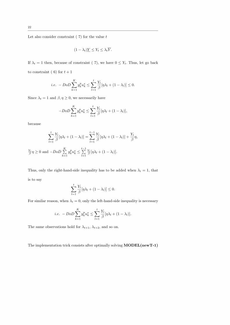
Let us consider constraint ( 6) for a fixed value of t

−DoDK∑

k=1

ypkusk ≤

t−1∑l=1

Yl

β[ηλl + (1− λl)] ≤ 0.

22

Let also consider constraint ( 7) for the value t

(1− λt)Y ≤ Yt ≤ λtY .

If λt = 1 then, because of constraint ( 7), we have 0 ≤ Yt. Thus, let go back

to constraint ( 6) for t+ 1

i.e. −DoD

K∑k=1

ypkusk ≤

t∑l=1

Yl

β[ηλl + (1− λl)] ≤ 0.

Since λt = 1 and β, η ≥ 0, we necessarily have

−DoDK∑

k=1

ypkusk ≤

t∑l=1

Yl

β[ηλl + (1− λl)],

because

t∑l=1

Yl

β[ηλl + (1− λl)] =

t−1∑l=1

Yl

β[ηλl + (1− λl)] +

Yt

βη,

Yt

β η ≥ 0 and −DoDK∑

k=1

ypkusk ≤

t−1∑l=1

Yl

β [ηλl + (1− λl)].

Thus, only the right-hand-side inequality has to be added when λt = 1, that

is to say

t∑l=1

Yl

β[ηλl + (1− λl)] ≤ 0.

For similar reason, when λt = 0, only the left-hand-side inequality is necessary

i.e. −DoDK∑

k=1

ypkusk ≤

t∑l=1

Yl

β[ηλl + (1− λl)].

The same observations hold for λt+1, λt+2, and so on.

The implementation trick consists after optimally solving MODEL(newT-1)

23

to discard all unnecessary inequalities in constraints ( 6), and associated lin-

earization variables in such a way to reduce the problem number of constraints.

One may observed also that fixing a binary variable λt is equivalent to fix

also the expression of the associated linearization variable xt. As a conse-

quence the problem size may be also reduced in terms of variables since all

variables xt may be replaced by their corresponding values : Yt (when λt = 1)

or 0 (when λt = 0).

Without these simple tricks it was not possible, for certain value of T′, in

our computing environment, to get enough memory to perform all iterations

of the algorithm.

5 Numerical results

The heuristic algorithm has been implemented for a real world case in a site

at Dakar (Senegal). The exact location of the site may be viewed in the figure

above (indication C : University Cheikh Anta Diop). The site is at 14◦41 N

Longitude, 17◦27 W Latitutde and 24 m sea level. Given some observations,

the practical objective of the experimentation is to size as better as possible

an Hybrid Renewable Energy System. Data related on environmental obser-

vations have been collected by colleagues of Ecole Superieure Polytechnique

de Dakar (ESP Dakar). Two of these important informations are the solar

radiations and wind speed over the observation period. Figure 6 show these

24

Fig. 5 Geographical Location in Dakar (Senegal)

informations. The wind speed is in average 4.3 m/s and the solar radiation is

in average (approximately) 200 W/m2.

Fig. 6 Observations

25

The number of types and the period length is given in the table 1.

T I J K

4343 2 2 2

Table 1 Period Length (T), Types (I,J,K)

Because of the huge value T , describing entirely the matrices P = {Pit}1≤i≤I0≤t≤T

and W = {Wjt}1≤j≤J0≤t≤T

, as well as the demand vector d = {dt}0≤t≤T in this

paper is of no interest.

The costs are in table 2. The maximum number of each renewable energy com-

ponents (i.e. values vpi , ypk, tj) has been fixed to 50. We also have DoD = 0.8,

β = 48 V olt and η = 0.8. The experiments have been performend on a PC Dell

with 2 G0 RAM, Intel Core Processor of 1.86 GHz and Linux Suze Operating

System. The linear programming model of each iteration has been solved with

Ilog Cplex 10.1.

In practice, the sizing process is done once. As a corollary, there is no ”strong

constraint” on the processing time. We are not necessarily searching for a

c1 c2 b1 b2 w1 w2

783.9 Eur. 675.1 Eur. 986.58 Eur. 2067.12 Eur. 27849.9 Eur. 23034.7 Eur.

Table 2 Costs

26

fast algorithm giving good solutions in few times but for an algorithm giving

”good” feasible solutions in a ”reasonable” amount of time. We have consid-

ered that more than 1000sec. (maximum fixed time limit at each iteration) for

solving exactly MODEL(newT− 1) at a iteration of the algorithm is urea-

sonable. When Cplex branch-and- bound iterates more that this time limit,

the processs is stop and we consider that our algorithm fails to find a solution

since MODEL(newT− 1) is supposed to be solved optimally.

A more flexible version of our heuristic may be to return in this case the

best integer integer solution found by Cplex and then to continue the heuris-

tic loop using this solution. This version was not explored in this paper. It will

be the subject of other computational experiments.

At the initial point of our heuristic (see subsection 4.1), a value for T′has

to be chosen. The values T′start with 100 and are increased by 50. The re-

sults are reported in table 3. For each T′the value of the first optimization is

stored in the column LB (Lower Bound). The objective function values at the

end of all iterations are in the column Cost, and the corresponding solutions

in the remaining columns. As explained in section 4.1 each value of the column

LB value is a lower bound of the optimal value of the problem. It follows that

the maximum value, noticed MaxLB of this column corresponds to the best

lower bound found. At the opposed, the minimal value of the column cost,

noticed MinCost, is the best solution found by the heuristic. Thus comparing

27

T′

LB Cost vp1 vp2 t1 t2 yp1 yp2 time (sec.)

100 69542.6 88791.1 40 1 0 0 4 1 1693.4

150 71491.6 80952.1 35 1 0 0 4 1 1309.92

200 71491.6 83652.8 39 1 0 0 1 2 1137.5

250 72678.2 88791.1 40 1 0 0 4 1 991.6

300 73870.1 82895.7 36 1 0 0 2 2 1063.7

350 73870.1 95486.3 36 1 0 0 1 4 1013

400 73870.1 89596.4 35 1 0 0 2 3 947.4

450 73870.1 85220.6 40 1 0 0 1 2 920.8

500 73870.1 93489.1 40 1 0 0 1 3 1305

550 78949.4 95438.1 44 1 0 0 2 2 946.9

600 78949.4 87599.1 39 1 0 0 2 2 875.6

650 78949.4 85220.6 40 1 0 0 1 2 976.7

700 78949.4 83276.9 39 1 0 0 3 1 1179.7

MinCost 80952.1

MaxLB 78949.4

Table 3 Numerical results

MaxLB and MinCost gives a idea of the quality of the heuristic.

In our experiments, the values of T′greater than 700 lead either to cplex

memory problem (CPLEX ERROR 1001 : Out of Memory) or ”unreason-

able” processing time (more than 1000sec. in a iteration) to solve optimally

MODEL(newT− 1). The best heuristic solution (MinCost) is equal to 80952.1.

For this solution the heuristic suggest to take no wind turbines, whatever

is the type, a type 1 (resp. type 2) PV array of size vp1vs1 = 35 ∗ 2 = 70

(resp. vp2vs2 = 1 ∗ 3 = 3) and a type 1 (resp. type 2) battery array of size

28

yp1ys1 = 4∗4 = 16 (resp. yp2y

s2 = 1∗4 = 4). The relative deviation with the best

lower bound, MaxLB, is equal to 80952.1−78949.478949.4 ∗100 ≈ 2.5%. So , we are not so

far from the optimal value but without garantee that we have really reached it.

The results correspond to meteorologic conditions and geographic location

of the site. Indeed, as attested by the wind speed graph, the wind exposure of

the site is low. For the types of turbines of this experiment, it is estimated (by

the specialists) that ”good” electrical production may be expected for wind

speed arround 6 m/s. The observations show that, in average, the wind speed

of the site is about 4.3 m/s. This is rather insufficient. And, taking into ac-

count the expensive costs (see table 2) of wind turbines, there is no evidence

for investment on such technologies. This may explain why the optimization

process suggests no wind turbines. At the opposed, because of significative

solar radiations of this geographical area, as well as competitive costs of solar

panels in comparison to wind turbines, the optimization suggests numerous

solar panels of each type. Thus, all of these results are not surprisingly and

show the practical validity of the model.

6 Conclusion and perspectives

In this paper, a quadratically constrained model for sizing an Hybrid Energy

Renewable System (HRES) was proposed. The goal of this system is to take

advantage of different weather conditions, geographic properties in such a way

to produce required electrical energy using various renewable energy sources.

29

Because of the very large size of the formulation, a heuristic has been pro-

posed to solve the model. The method proposed may be classified in referent

domain based optimization method [4]. The formulation has been used with

data collected in a Dakar site. The results are consistent in the light of the

meteorological informations on this site.

However, because of the heuristic approach, optimality of this solution is not

guarantee. It remains to compute a lower bound in order to evaluate the qual-

ity of the solution. We have seen above that using simply a linear relaxation do

not work in our computing environment because of memory problem resulting

by the very large scale integer linear problem. In further researches, we seek

to fix this point with decomposition methods exploiting the specific structure

of the constraints, in particular constraints 6.

Another interesting perspective is to take into account the stochastic nature

of the problem. All data used in the model have been supposed deterministics

using some approximations. It is well known that meteorologic conditions are

stochastic and since the energy produced by solar panels or wind turbines de-

pends on these conditions then the power of a solar panel of type i at time t

(i.e Pit) and the power of a wind turbine of type j at time t (i.e Wjt) should be

stochastic variables. Our perspective in this field will deal to propose stochastic

programming modeling and associated resolution scheme.

30

Acknowledgements The authors would like to thank Badara Mboup, Asssistant Professor

at Ecole Superieure Polytechnique (ESP) de Dakar (Senegal), for collecting and providing

data, making possible numerical experiments.

References

1. R. Belfkira, G. Barakat, and C. Nichita. Sizing optimization of a stand-

alone hybrid power supply unit : Wind/pv system with battery storage.

International Review of Electrical Engineering (IREE), 3(5):820–828, 2008.

2. A. Billionnet. Optimisation discrete - De la modelisation a la resolution

par des logiciels de programmation mathematique. Dunod, 2007.

3. R. Fortet. Applications de l’algebre de boole en recherche

operationnelle. Revue Francaise d’Automatique, d’Informatique et de

Recherche Operationnelle, 4:5–36, 1959.

4. F. Glover and F. Laguna. Tabu Search. Kluwer Academic Publisher, 1997.