A Pull Planning Frameworkweb.utk.edu/~kkirby/IE515/Ch13.pdfA Pull Planning Framework We think in...

1

1© Wallace J. Hopp, Mark L. Spearman, 1996, 2000 http://factory-physics.com

A Pull Planning Framework

We think in generalities, we live in detail.

–Alfred North Whitehead


Purpose of Production Control

Objective: Meet customer expectations with on-time delivery of correctquantities of desired specification without excessive lead times orlarge inventory levels.

Two Basic Approaches:

Push Systems: Material Requirements Planning

• General.

• Provides a planning hierarchy.

• Underlying model often inappropriate.

Pull Systems: Kanban

• Reduces congestion.

• Improves production environment.

• Suitable only for repetitive manufacturing.

2


Advantages of Pull

Advantages:

• Observability: we can see WIP but not capacity.

• Efficiency: pull systems require less average WIP to attain samethroughput as equivalent push system.

• Robustness: pull systems are less sensitive to errors in WIP levelthan push systems are to errors in release rate.

• Quality: pull systems require and promote improved quality.

Magic of Pull: WIP CapWIP


A Dilemma

Question: If pull is so great, why do people still buy ERP systems?

Answer: Manufacturing involves planning as well as execution.

Planning Execution

Push good bad

Pull bad goodExecution

3


MRP II Planning Hierarchy

DemandForecast

Aggregate ProductionPlanning

Master ProductionScheduling

Material RequirementsPlanning

JobPool

JobRelease

JobDispatching

Capacity RequirementsPlanning

Rough-cut CapacityPlanning

ResourcePlanning

RoutingData

InventoryStatus

Bills ofMaterial


Hierarchical Pull Planning Framework

Goals:• To attain the benefits of a pull environment.

• To gain the generality of hierarchical production planning systems.

The Environment:• CONWIP production lines.

• Daily/Weekly production quota.

The Hierarchy:

• Based on CONWIP for predictability and generality.

• Consistency between levels.

• Accommodate different implementations of modules for differentenvironments.

• Use feedback.

4


Hierarchical Planning in a Pull System

PersonnelPlan

FORECASTING

CAPACITY/FACILITYPLANNING

WORKFORCE PLANNING

MarketingParameters

Product/ProcessParameters

LaborPolicies

CapacityPlan

AGGREGATEPLANNING

AggregatePlan Strategy

WorkSchedule

WIP/QUOTASETTING

DEMANDMANAGEMENT

SEQUENCING & SCHEDULING

CustomerDemands

MasterProductionSchedule

SHOP FLOORCONTROL

WIPPosition Tactics

REAL-TIMESIMULATION

PRODUCTIONTRACKING

WorkForecast

Control


CONWIP as the Foundation

Pull:• jobs into the line whenever parts are used.

• jobs with the same routing.

• jobs for different part numbers.

Push:• jobs between stations on line.

• jobs into buffer storage between lines.

A CONWIP Line:• represents a level in a bill of material.

• is between stock points.

• maintains a constant amount of work in process.

CONWIP

5


Benefits of CONWIP

CONWIP vs. Push:• Easier and more robust control.

• Less congestion.

• Greater predictability.

CONWIP vs. Kanban:• Can accommodate a changing product mix.

• Can be used with setups.

• Suitable for short runs of small lots.

• More predictable.

. . .

. . .

…

. . .


Conveyor Model of CONWIP

Predicting Completion Times:• Practical production rate: rP parts per hour

• Minimum practical lead time: TP hours

• Xi is number of parts in job i on the backlog.

• Then the expected completion time of the nth job, cn, will be:

Quoting Due Dates: need to add a “fudge factor” (which shouldconsider cycle time variability) to ensure a reasonable service level.

PP

n

i i

n Tr

Xc += ∑ =1

TP

n rP

6


Aggregating Planning by Time Horizon

Time Horizon Length Representative DecisionsLong-Term(Strategy)

year – decades Financial DecisionsMarketing StrategiesProduct DesignsProcess Technology DecisionsCapacity DecisionsFacility LocationsSupplier ContractsPersonnel Development ProgramsPlant Control PoliciesQuality Assurance Policies

Intermediate-Term(Tactics)

week – year Work SchedulingStaffing AssignmentsPreventive MaintenanceSales PromotionsPurchasing Decisions

Short-Term(Control)

hour – week Material Flow ControlWorker AssignmentsMachine Setup DecisionsProcess ControlQuality Compliance DecisionsEmergency Equipment Repairs


Other Levels of Aggregation

Processes: Treat several workstations as one. Leave out unimportant (neverbottleneck) workstations.

Products: Group different part numbers into product families, which have

• have roughly the same routing

• have roughly the same price

• share setups

Personnel: Categorize people according to

• management vs. labor

• shift

• workstation

• craft

• permanent vs. temporary

7


Forecasting

Basic Problem: predict demand for planning purposes.

Laws of Forecasting:1. Forecasts are always wrong!

2. Forecasts always change!

3. The further into the future, the less reliable the forecast will be!

Forecasting Tools:• Qualitative:

– Delphi

– Analogies

– Many others

• Quantitative:– Causal models (e.g., regression models)

– Time series models


Capacity/Facility Planning

Basic Problem: how much and what kind of physical equipment isneeded to support production goals?

Issues:

• Basic Capacity Calculations: stand-alone capacities andcongestion effects (e.g., blocking)

• Capacity Strategy: lead or follow demand

• Make-or-Buy: vendoring, long-term identity

• Flexibility: with regard to product, volume, mix

• Speed: scalability, learning curves

8


Workforce Planning

Basic Problem: how much and what kind of labor is needed to supportproduction goals?

Issues:

• Basic Staffing Calculations: standard labor hours adjusted forworker availability.

• Working Environment: stability, morale,learning.

• Flexibility/Agility: ability of workforce tosupport plant's ability to respond to shortand long term shifts.

• Quality: procedures are only as goodas the people who carry them out.


Aggregate Planning

Basic Problem: generate a long-term production plan that establishes arough product mix, anticipates bottlenecks, and is consistent withcapacity and workforce plans.

Issues:

• Aggregation: product families and time periods must be setappropriately for the environment.

• Coordination: AP is the link between the high level functions offorecasting/capacity planning and intermediate level functions ofquota setting and scheduling.

• Anticipating Execution: AP is virtually always donedeterministically, while production is carried out in a stochasticenvironment.

• Linear Programming: is a powerful tool well-suited to AP andother optimization problems.

9


Quota Setting

Basic Problem: set target production quota for pull system

Issues: Larger quotas yield

Benefits:• Increased throughput.

• Increased utilization.

• Lower unit labor hour.

• Lower allocation of overhead.

Costs:• More overtime.

• Higher WIP levels.

• More expediting.

• Increased difficulties in quality control.


Planned Catch-Up Times

RegularTime

R0

Catch-UpRegular

TimeCatch-Up

T T+R 2T

10


Economic Production Quota Notation

variable)(decision quota production meregular ti

production overtime maximum

))(( production meregular ti of dev std

])[( production meregular timean

variable)(random production meregular ti

cost overtime fixed

profitunit

===

====

Q

M

YVar

YE

Y

C

p

OT


Simple “Sell-All-You-Can-Make” Model

Objective Function: Average weekly profit

Reasonability Test: We want the probability of not being able to catchup on overtime to be small (i.e., ):

If this is not true, another (lost sales) model should be used.

}Pr{max QYCpQZ OTQ

≤−=

≤>− }Pr{ * MYQ

11


Simple “Sell-All-You-Can-Make” Model (cont.)

Normal Approximation: Express Q = - k , so the objective and

reasonability test can be written:

Solution: The objective function is maximized by:

−≥+Φ

Φ−−−=

1)/(

))(1()(max

Mk

kCkpZ OTk

**

*

2ln2

kQ

p

Ck OT

−=

=

buffer capacity


Intuition from Model

• Optimal production quota depends on both mean and variance of regulartime production (Q* increases with and decreases with ).

• Increasing capacity increases profit, since

• Decreasing variance increases profit, since

• Model is valid (i.e., has a solution 0 < k* < ∞) only if

since otherwise the term in the √ becomes negative. If this occurs, then

OT cost does not exceed revenue lost to make-up period and a differentmodel is required.

pZ =

∂∂ *

**

pkZ −=

∂∂

2OTC

p ≤

12


Other Quota Setting Models

Model 2: Lost Sales

• Run continuously.

• Choose periodic production quota Q.

• Demand above Q is lost (or vendored) at a cost.

• Solution looks like that to the Newsboy problem

Model 3: Fixed plus Variable Cost of Overtime

• Same as Model 1, except that cost of overtime has a fixedcomponent, COT, and a component proportional to the amount ofthe shortage

• Solution looks like that to Model 1 except term under √ is more

complex


Other Quota Setting Models (cont.)

Model 4: Backlogging

• Fixed plus variable cost of overtime.

• Decision maker can choose to carry shortage to next period at acost

• Dependence between periods requires more sophisticated solutiontechniques (e.g., dynamic programming).

• Solution consists of Q*, optimal quota, plus S*, an “overtimetrigger” such that we use overtime only if the shortage is at least S.

13


Quota Setting Implementation

• Iteration between quota setting and aggregate planning may benecessary for consistency.

• Motivation (setting the “bar”) vs. Prediction (quoting due dates).

• MPS smoothing – necessary to keep steady quota.

• Gross capacity control through shift addition/deletion, rather thanproduction slow-down.


Setting WIP Levels

Basic Problem: establish WIP levels (card counts) in pull system.

Issues:• Mean regular time production increases with WIP level.

• Variance of regular time production also affected by WIP level.

• WIP levels should be set to facilitate desired throughput.

• Adjustment may be necessary as system evolves (feedback).

• Easy method:1. Specify feasible cycle time, CT, and identify practical production rate,

rP.

2. Set WIP from

WIP = rP × CT

14


Demand Management

Basic Problem: establish an interface between the customer and theplant floor, that supports both competitive customer service andworkable production schedules.

Issues:

• Customer Lead Times: shorter is more competitive.

• Customer Service: on-time delivery.

• Batching: grouping like product families can reduce lost capacitydue to setups.

• Interface with Scheduling: customer due dates are are anenormously important control in the overall scheduling process.


Sequencing and Scheduling

Basic Problem: develop a plan to guide the release of work into thesystem and coordination with needed resources (e.g., machines,staffing, materials).

Methods:• Sequencing:

– Gives order of releases but not times.

– Adequate for simple CONWIP lineswhere FISFO is maintained.

– The “CONWIP backlog.”

• Scheduling:– Gives detailed release times.

– Attractive where complex routings make simple sequence impractical.

– MRP-C.

15


Sequencing CONWIP Lines

Objectives:• Maximize profit.

• No late jobs.

• All firm jobs selected.

Job Sequencing System:• Sequences bottleneck line.

• Uses Quota to explicitly consider capacity.

• Tries to group like families of jobs to reduce setups.

• Identifies the “offensive” jobs in an infeasible schedule.

• Suggests when more work could start in a lightly loaded schedule.

• Provides sequence for other lines.

PN Quant–— ––––––— ––––––— ––––––— ––––––— ––––––— ––––––— ––––––— ––––––— ––––––— ––––––— ––––––— ––––––— –––––

Work Backlog

LAN

. . .


Real-Time Simulation

Basic Problem: anticipate problems in schedule execution and providevehicle for exploring solutions.

Approaches:

• Deterministic Simulation:– Given release schedule and dispatching rules, predict output times.

– Commercial packages (e.g., FACTOR).

• Conveyor Model:– Allow hot jobs to pass in buffers, not in the lines.

– Use simplified simulation based on conveyor model. to predict outputtimes.

16


Shop Floor Control

Basic Problem: control flow of work through plant and coordinate withother activities (e.g., quality control, preventive maintenance, etc.)

Issues:

• Customization: SFC is often the most highly customized activityin a plant.

• Information Collection: SFC represents the interface with theactual production processes and is therefore a good place to collectdata.

• Simplicity: departures from simple mechanisms must be carefullyjustified.


Tracking and Feedback

Basic Problems:• Signal quota shortfall.

• Update capacity data.

• Quote delivery dates.

Functions:

Statistical Throughput Control:• Monitored at critical tools.

• Like SPC, only measuring throughput.

• Problems are apparent with time to act.

• Workers aware of situation.

Feedback:• Collect capacity data.

• Measure continual improvement.

17


Conclusions

Pull Environment Provides:• Less WIP and thereby earlier detection of quality problems.

• Shorter lead times allowing increased customer response and lessreliance on forecasts.

• Less buffer stock and therefore less exposure to schedule andengineering changes.

CONWIP Provides: a pull environment that

• Has greater throughput for equivalent WIP than kanban.

• Can accommodate a changing product mix.

• Can be used with setups.

• Is suitable for short runs of small lots.

• Is predictable.


Conclusions (cont.)

Planning Hierarchy Provides:• Consistent framework for planning.

• Links between levels.

• Feedback.

18


Forecasting

The future is made of the same stuff as the present.

– Simone Weil


Forecasting “Laws”

1) Forecasts are always wrong!

2) Forecasts always change!

3) The further into the future, the less reliable the forecast!

Start ofseason

20%

40%

+10%

-10%

16 weeks

26 weeks

Trumpet of Doom

19


Quantitative Forecasting

Goals:• Predict future from past• Smooth out “noise”• Standardize forecasting procedure

Methodologies:• Causal Forecasting:

– regression analysis– other approaches

• Time Series Forecasting:– moving average– exponential smoothing– regression analysis– seasonal models– many others


Time Series Forecasting

Time series modelA(i), i = 1, … ,t

ForecastHistorical Data

f(t+t), i = 1, 2, …

20


Time Series Approach

Notation:

ttT

ttF

ttf

t

iiA

period of as trendsmoothed)(

period of as estimate smoothed)(

periodfor forecast )(

periodcurrent

periodin n observatio)(

==

+=+==


Time Series Approach (cont.)

Procedure:1. Select model that computes f(t+τ) from A(i), i = 1, … , t

2. Forecast existing data and evaluate quality of fit by using:

3. Stop if fit is acceptable. Otherwise, adjust model constants and goto (2) or reject model and go to (1).

∑

∑

∑

=

=

=

−=

−=

−=

n

t

n

t

n

t

ntAtf

ntAtf

ntAtf

1

1

2

1

))()((BIAS

))()((MSD

)()(MAD

21


Moving Average

Assumptions:• No trend

• Equal weight to last m observations

Model:

... 2, ,1),()(

)()( 1

==+

= ∑ =

tFtf

t

iAtF

t

i


Moving Average (cont.)

Example: Moving Average with m = 3 and m = 5.

Month t

Demand A (t )

Forecast (m =3) f (t )

Forecast (m =5) f (t )

1 10 - -2 12 - -3 12 - -4 11 11.33 -5 15 11.67 -6 14 12.67 12.07 18 13.33 12.88 22 15.67 14.09 18 18.00 16.0

10 28 19.33 17.411 33 22.67 20.012 31 26.33 23.813 31 30.67 26.414 37 31.67 28.215 40 33.00 32.016 33 36.00 34.417 50 36.67 34.418 45 41.00 38.219 55 42.67 41.020 60 50.00 44.6

Note: biggerm makes forecastmore stable, butless responsive.

22


Exponential Smoothing

Assumptions:• No trend

• Exponentially declining weight given to past observations

Model:

... 2, ,1),()(

)1()1()()(

==+

−−+=

tFtf

tFtAtF


Exponential Smoothing (cont.)

Example: Exponential Smoothing with α = 0.2 and α = 0.6.

Month t

Demand A (t )

Forecast ( =0.2) f (t )

Forecast ( =0.6) f (t )

1 10 - -2 12 10.00 10.003 12 10.40 11.204 11 10.72 11.685 15 10.78 11.276 14 11.62 13.517 18 12.10 13.808 22 13.28 16.329 18 15.02 19.73

10 28 15.62 18.6911 33 18.09 24.2812 31 21.08 29.5113 31 23.06 30.4014 37 24.65 30.7615 40 27.12 34.5016 33 29.69 37.8017 50 30.36 34.9218 45 34.28 43.9719 55 36.43 44.5920 60 40.14 50.83

Note: we are still lagging behind actualvalues.

23


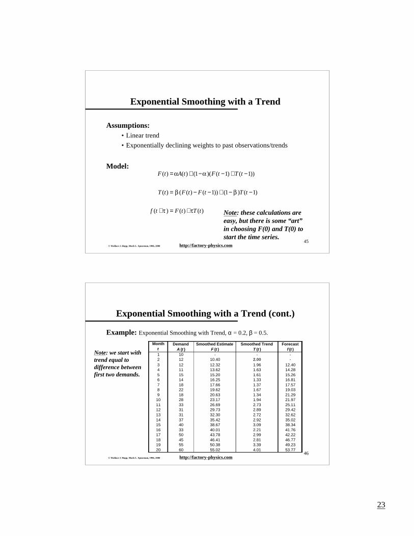
Exponential Smoothing with a Trend

Assumptions:• Linear trend

• Exponentially declining weights to past observations/trends

Model:

)()()(

)1()1())1()(()(

))1()1()(1()()(

tTtFtf

tTtFtFtT

tTtFtAtF

+=+

−−+−−=

−+−−+=

Note: these calculations areeasy, but there is some “art”in choosing F(0) and T(0) tostart the time series.


Exponential Smoothing with a Trend (cont.)

Example: Exponential Smoothing with Trend, α = 0.2, β = 0.5.

Month t

Demand A (t )

Smoothed Estimate F (t )

Smoothed Trend T (t )

Forecast f (t )

1 10 - - -2 12 10.40 2.00 -

3 12 12.32 1.96 12.404 11 13.62 1.63 14.285 15 15.20 1.61 15.266 14 16.25 1.33 16.817 18 17.66 1.37 17.578 22 19.62 1.67 19.039 18 20.63 1.34 21.29

10 28 23.17 1.94 21.9711 33 26.69 2.73 25.1112 31 29.73 2.89 29.4213 31 32.30 2.72 32.6214 37 35.42 2.92 35.0215 40 38.67 3.09 38.3416 33 40.01 2.21 41.7617 50 43.78 2.99 42.2218 45 46.41 2.81 46.7719 55 50.38 3.39 49.2320 60 55.02 4.01 53.77

Note: we start with trend equal to difference betweenfirst two demands.

24


Exponential Smoothing with a Trend (cont.)

Example: Exponential Smoothing with Trend, α = 0.2, β = 0.5.

Month t

Demand A (t )

Smoothed Estimate F (t )

Smoothed Trend T (t )

Forecast f (t )

1 10 10.00 0.00 -2 12 10.40 0.20 -3 12 10.88 0.34 10.604 11 11.18 0.32 11.225 15 12.20 0.67 11.496 14 13.09 0.78 12.867 18 14.70 1.19 13.878 22 17.11 1.81 15.899 18 18.74 1.71 18.92

10 28 21.96 2.47 20.4511 33 26.14 3.33 24.4312 31 29.77 3.48 29.4713 31 32.80 3.25 33.2514 37 36.25 3.35 36.0615 40 39.67 3.39 39.5916 33 41.05 2.38 43.0617 50 44.75 3.04 43.4318 45 47.23 2.76 47.7919 55 50.99 3.26 49.9920 60 55.40 3.84 54.25

Note: we start with trend equal to zero.


Effects of Altering Smoothing Constants

Exponential Smoothing with Trend: various values of α and β

MAD MSD BIAS

0.1 0.2 4.11 27.56 -2.000.1 0.4 3.98 24.82 -1.940.1 0.6 3.76 21.98 -1.730.1 0.8 3.63 20.07 -1.470.1 1.0 3.54 19.26 -1.200.4 0.2 3.75 21.82 -1.070.4 0.4 3.83 22.52 -0.850.4 0.6 3.93 23.87 -0.780.4 0.8 4.01 24.82 -0.740.4 1.0 4.08 25.44 -0.670.7 0.2 4.34 27.18 -0.750.7 0.4 4.53 30.00 -0.600.7 0.6 4.74 33.65 -0.500.7 0.8 4.99 38.39 -0.410.7 1.0 5.27 44.59 -0.341.0 0.2 4.94 39.82 -0.561.0 0.4 5.25 48.75 -0.421.0 0.6 5.83 61.27 -0.321.0 8.0 6.66 78.86 -0.251.0 1.0 7.72 104.06 -0.17

Note: these assumewe start with trendequal diff betweenfirst two demands.

25


Effects of Altering Smoothing Constants

Exponential Smoothing with Trend: various values of α and β

Note: these assume we start with trend equal to zero.

MAD MSD BIAS MAD MSD BIAS0.1 0.1 10.23 146.94 -10.23 0.4 0.1 4.3 30.14 -3.45

0.1 0.2 8.27 95.31 -8.27 0.4 0.2 3.89 23.78 -2.340.1 0.3 6.83 64.91 -6.69 0.4 0.3 3.77 22.25 -1.770.1 0.4 5.83 47.17 -5.43 0.4 0.4 3.75 22.11 -1.46

0.1 0.5 5.16 36.88 -4.42 0.4 0.5 3.76 22.36 -1.290.1 0.6 4.69 30.91 -3.62 0.4 0.6 3.79 22.67 -1.18

0.2 0.1 6.48 60.55 -6.29 0.5 0.1 4.13 27.4 -2.840.2 0.2 5.04 37.04 -4.49 0.5 0.2 3.91 23.61 -1.94

0.2 0.3 4.26 27.56 -3.29 0.5 0.3 3.88 23.02 -1.490.2 0.4 3.9 23.75 -2.51 0.5 0.4 3.9 23.26 -1.25

0.2 0.5 3.73 22.32 -2.02 0.5 0.5 3.94 23.73 -1.10.2 0.6 3.65 21.94 -1.71 0.5 0.6 3.97 24.27 -10.3 0.1 4.98 37.81 -4.45 0.6 0.1 4.12 26.85 -2.42

0.3 0.2 4.11 26.3 -3.03 0.6 0.2 4.03 24.63 -1.660.3 0.3 3.82 22.74 -2.23 0.6 0.3 4.04 24.69 -1.29

0.3 0.4 3.66 21.81 -1.77 0.6 0.4 4.09 25.35 -1.080.3 0.5 3.65 21.78 -1.52 0.6 0.5 4.14 26.25 -0.95

0.3 0.6 3.68 22.06 -1.38 0.6 0.6 4.21 27.29 -0.84


Effects of Altering Smoothing Constants (cont.)

Observations: assuming we start with zero trend

• α = 0.3, β = 0.5 work well for MAD and MSD

• α = 0.6, β = 0.6 work better for BIAS

• Our original choice of α = 0.2, β = 0.5 had MAD = 3.73, MSD =

22.32, BIAS = -2.02, which is pretty good, although α = 0.3, β =

0.6, withMAD = 3.65, MSD=21.78, BIAS = -1.52 is better.

26


Winters Method for Seasonal Series

Seasonal series: a series that has a pattern that repeats every N periodsfor some value of N (which is at least 3).

Seasonal factors: a set of multipliers ct , representing the averageamount that the demand in the tth period of the season is above orbelow the overall average.

Winter’s Method:• The series:

• The trend:

• The seasonal factors:

• The forecast:

)1()1()(1()(/)(()( −+−−+−= tTtFNtctAtF

)1()1()1()(()( −−+−−= tTtFtFtT

)()1())(/)(()( NtctFtAtc −−+=

)())()(()( tctTtFtf +=+


Winters Method ExampleYear Quarter t A(t) F(t) T(t) c(t) f(t) f(t)-A(t) |f(t)-A(t)|(f(t)-A(t))^2

1997 1 1 4 --- --- 0.4802 2 2 --- --- 0.2403 3 5 --- --- 0.6004 4 8 --- --- 0.9605 5 11 --- --- 1.3206 6 13 --- --- 1.5607 7 18 --- --- 2.1608 8 15 --- --- 1.8009 9 9 --- --- 1.08010 10 6 --- --- 0.72011 11 5 --- --- 0.60012 12 4 8.33 0.00 0.480

1998 1 13 5 8.54 0.02 0.491 4.00 -1.00 1 1.002 14 4 9.37 0.10 0.259 2.06 -1.95 1.945 3.783 15 7 9.69 0.12 0.612 5.68 -1.32 1.31513 1.734 16 7 9.57 0.10 0.937 9.43 2.43 2.42506 5.885 17 15 9.83 0.12 1.341 12.76 -2.24 2.24392 5.046 18 17 10.04 0.13 1.573 15.52 -1.48 1.47921 2.197 19 24 10.26 0.13 2.178 21.97 -2.03 2.03484 4.148 20 18 10.36 0.13 1.794 18.72 0.72 0.71585 0.519 21 12 10.55 0.14 1.086 11.33 -0.67 0.67254 0.4510 22 7 10.59 0.13 0.714 7.69 0.69 0.69489 0.4811 23 8 10.98 0.15 0.613 6.43 -1.57 1.56928 2.4612 24 6 11.27 0.17 0.485 5.34 -0.66 0.65635 0.43

alpha 0.100 -0.76 1.40 2.34beta 0.100 bias MAD MSD

gamma 0.100

27


Winters Method - Sample Calculations

33.812

424

12

)(

)12(

12

1 =+++==∑

= Lt

tA

F

480.033.8

4

)12(

)1()1( ===

F

Ac

54.8)033.8)(1.01()480.0/5(1.0

))12()12()(1()1213(/)13(()13(

=+−+=+−+−= TFcAF

02.0)0)(1.01()33.854.8(1.0

)12()1())12()13(()13(

=−+−=−+−= TFFT

491.0)48.0)(1.01()54.8/5((1.0

)1()1())13(/)13(()13(

=−+=−+= cFAc

Initially we set:• smoothed estimate = first season average• smoothed trend = zero (T(N)=T(12) = 0)• seasonality factor = ratio of actual to average demand

From period 13 on we can useinitial values and standard formulas...


Winters Method Example

0

5

10

15

20

25

0 1 2 3 4 5 6 7 8 9 10 11 12 13 14 15 16 17 18 19 20 21 22 23 24

Month

Dem

an

d

A(t)

f(t)

28


Conclusions

Sensitivity: Lower values of m or higher values of α will make movingaverage and exponential smoothing models (without trend) more sensitive todata changes (and hence less stable).

Trends: Models without a trend will underestimate observations in time serieswith an increasing trend and overestimate observations in time series with adecreasing trend.

Smoothing Constants: Choosing smoothing constants is an art; the bestwe can do is choose constants that fit past data reasonably well.

Seasonality: Methods exist for fitting time series with seasonal behavior(e.g., Winters method), but require more past data to fit than the simplermodels.

Judgement: No time series model can anticipate structural changes notsignaled by past observations; these require judicious overriding of the modelby the user.

A Pull Planning Frameworkweb.utk.edu/~kkirby/IE515/Ch13.pdfA Pull Planning Framework We think in...

Documents

Transcript of A Pull Planning Frameworkweb.utk.edu/~kkirby/IE515/Ch13.pdfA Pull Planning Framework We think in...