A Project Scheduling Approach To Production Planning with ...

HAL Id: hal-00576097https://hal.archives-ouvertes.fr/hal-00576097

Submitted on 12 Mar 2011

HAL is a multi-disciplinary open accessarchive for the deposit and dissemination of sci-entific research documents, whether they are pub-lished or not. The documents may come fromteaching and research institutions in France orabroad, or from public or private research centers.

L’archive ouverte pluridisciplinaire HAL, estdestinée au dépôt et à la diffusion de documentsscientifiques de niveau recherche, publiés ou non,émanant des établissements d’enseignement et derecherche français ou étrangers, des laboratoirespublics ou privés.

A Project Scheduling Approach To Production Planningwith Feeding Precedence Relations

Arianna Alfieri, Marcello Urgo, Tullio Tolio

To cite this version:Arianna Alfieri, Marcello Urgo, Tullio Tolio. A Project Scheduling Approach To Production Planningwith Feeding Precedence Relations. International Journal of Production Research, Taylor & Francis,2010, pp.1. �10.1080/00207541003604844�. �hal-00576097�

https://hal.archives-ouvertes.fr/hal-00576097

https://hal.archives-ouvertes.fr

For Peer Review O

nly

A Project Scheduling Approach To Production Planning with

Feeding Precedence Relations

Journal: International Journal of Production Research

Manuscript ID: TPRS-2009-IJPR-0674.R1

Manuscript Type: Original Manuscript

Date Submitted by the Author:

20-Dec-2009

Complete List of Authors: Alfieri, Arianna; Politecnico di Torino, Production Systems and Economics Department Urgo, Marcello; Politecnico di Milano, Manufacturing and Production Systems Division, Department of Mechanical Engineering Tolio, Tullio; National Research Council, Institute of Industrial Technologies and Automation

Keywords: PRODUCTION PLANNING, PROJECT SCHEDULING

Keywords (user): FEEDING PRECEDENCE RELATIONS

http://mc.manuscriptcentral.com/tprs Email: [email protected]

International Journal of Production Research

For Peer Review O

nly

International Journal of Production ResearchVol. 00, No. 00, 00 Month 200x, 1–29

RESEARCH ARTICLE

A Project Scheduling Approach To Production Planning with

Feeding Precedence Relations

Arianna Alfieria, Tullio Toliob and Marcello Urgoc∗

aProduction Systems and Economics Department, Politecnico di Torino, Torino, Italy;bInstitute of Industrial Technologies and Automation, National Research Council,

Milano, Italy; cManufacturing and Production Systems Division, Department of

Mechanical Engineering, Politecnico di Milano, Milano, Italy

()

In Manufacturing-to-Order or Engineering-to-Order systems producing complex and highlycustomized items, each item has its own characteristics,which are often tailored for a spe-cific customer. Project scheduling approaches are suitable for production planning in suchenvironments. However, when we consider the production of complex items, thedistinct production operations are often aggregated into activities representingwhole production phases. In such cases, the planning and scheduling problemworks on the aggregate activities, considering that, in most cases, such activitiesalso have to be manually executed. Moreover, simple finish-to-start precedence relationsno longer correctly represent the real production process, but overlapping among activitiesshould be allowed. In this paper, a project scheduling approach is proposed for productionplanning in Manufacturing-to-Order systems. The Variable Intensity formulation is used toallow the effort committed to the execution of activities to vary over time. Feeding prece-dences are developed to model generalized precedence relations when the execution mode ofactivities is not known a priori. Two mathematical formulations of these precedence relationsare proposed. The formulations are applied both to random generated instances and to anindustrial system producing machining centers and are compared in terms of computationalefficiency.

Keywords: production planning, project scheduling, feeding precedence relations.

1. Introduction

The use of project scheduling approaches for production planning have been fre-quently addressed in the scientific literature (Klein 2000, Markus et al. 2003). Inparticular, when hierarchical planning approaches are used, project scheduling canserve as a planning tool at certain aggregate levels (Neumann and Schwindt 1998,Neumann et al. 2003). Project scheduling approaches for production planning areespecially important and useful when particular kinds of production environmentsare considered. In Manufacturing-to-Order (MTO) or Engineering-to-Order (ETO)systems producing complex and highly customized items, for example, each itemhas its own characteristics, which are often tailored for a specific customer. Thedesign, production and delivery to the customer of each product is then a one ofa kind activity that can be easily modeled as the execution of a project. In theproduction plant, different projects are executed together, competing for the sameproduction resources (machines, workers, etc.).

∗Corresponding author. Email: [email protected]

ISSN: 0020-7543 print/ISSN 1366-588X onlinec© 200x Taylor & FrancisDOI: 10.1080/00207540xxxxxxxxxhttp://www.informaworld.com

Page 1 of 40



123456789101112131415161718192021222324252627282930313233343536373839404142434445464748495051525354555657585960

For Peer Review O

nly

2

In production planning, project scheduling approaches must usually refer to amedium or long time horizon to provide an adequate view on the future activities.As in hierarchical planning and scheduling approaches, it is appropriate for a pro-duction planning approach to work on an aggregate level without considering all thescheduling details. Hence, distinct production operations can be grouped into ag-gregate activities, and machines and workers are considered together to constituteproduction resources. The aggregate activities often represent whole productionphases, and their duration can be significant. Moreover, planning on an aggregatelevel can also be an unescapable choice when a detailed production process is notknown or is difficult to define at the production planning level.

The use of a project scheduling approach at the aggregate production planninglevel has been described by Hans (2001), where it is called the aggregate (tactical)capacity planning problem or resource loading problem. At this aggregate level, aplanner can plan production subject to capacity requirements over a time horizon ofseveral weeks to several months, and thus can quote reliable due dates to customers.

Though it takes an aggregate view of the production activities, project schedulingapproaches still consider precedence relations among aggregate activities togetherwith resource loads, and hence they are more likely to provide feasibility at thedetailed scheduling phase than the usual rough cut capacity planning approacheswhen applied to these kinds of production systems (i.e., MTO and ETO). Theinadequacy of existing hierarchical planning approaches is often due to the factthat material-oriented (MRP/MRP II systems) or capacity-oriented (HPP sys-tems) issues are kept separate (Zijm 2000). The integration of capacity planningand material coordination achieved by project scheduling approaches to productionplanning can provide a solution to these problems in particular types of productionenvironments.

In Neumann and Schwindt (1998) and Neumann et al. (2003), a three-level hier-archical multi-project planning approach is presented to deal with make-to-ordersystems. At the first level of the proposed hierarchical approach, a portfolio oflong-term projects (orders) is to be planned and executed within a medium/longplanning horizon. Each project has a work breakdown structure consisting of aggre-gate activities to be scheduled subject to scarce key resources, and their durationis estimated by the critical-path length of the corresponding subprojects plus atime buffer. The resource requirement for an aggregate activity is computed as theratio between the total workload of the corresponding subproject and its estimatedduration. A fixed execution mode is considered, and the execution constraints aremodeled using generalized precedence relations.

In contrast, project scheduling at an aggregate level leads to some difficulties inthe definition of precedence relations among the activities (Vancza et al. 2004).Considering a single manufacturing operation, it is easy to define a finish-to-startprecedence relation representing technological constraints. However, when the op-erations are grouped into aggregate activities, the finish-to-start relations might nolonger correctly represent the real production process. In these cases, a commonapproach to model the precedence relations more accurately is to use GeneralizedPrecedence Relations (GPRs) (Elmaghraby 1977, Elmaghraby and Kamburowski1992) that allow a certain amount of overlap among activities. GPRs have beenextensively considered in the literature on project scheduling to model complexprecedence structures in activity networks (Demeulemeester and Herroelen 1997,Neumann and Schwindt 1997, De Reyck and Herroelen 1999, Klein 2000).

A further issue in MTO/ETO systems is the presence of manually executed activ-ities. FFor these activities, the concepts of unary resources and activity durationsneed to be reassessed. A single worker, in fact, can be assigned to different activi-

Page 2 of 40



123456789101112131415161718192021222324252627282930313233343536373839404142434445464748495051525354555657585960

For Peer Review O

nly

3

ties in the same time period, and, at the same time, more workers can be assignedto the same activity. Hence, either the resource used in each time period, or theduration of the activity, are not univocally defined, which makes the traditionalscheduling methods no longer suitable. In the literature, the Variable Intensityformulation of the Resource Constrained Project Scheduling problem is proposedto deal with such cases. In this formulation, an intensity variable is introduced todefine the effort dedicated to process each activity in each time period (Leachmanet al. 1990, Kis 2005). Resources (considered continuously divisible) are allocatedto activities in quantities that vary over time.

A further criticality arises when using the variable intensity formulation togetherwith generalized precedence relations. Due to the introduction of the intensityvariable, an infinite number of execution modes are allowed for the activities. Hence,the execution progress of each activity is not fixed but depends on its executionmode, and GPRs can no longer exhaustively describe the overlap among activities(Kis 2006, Tolio and Urgo 2007).

The concept of Feeding Precedence Relation, introduced by Kis (2005), has beendeveloped precisely to overcome the difficulties described above. However, Kis onlydefines a single type of feeding precedence relation, to constrain an activity to startonly after a certain percentage of its predecessor activity has been completed. Thistype of feeding precedence relation has been modeled through binary variablescalled the execution mask and solved through an ad-hoc Branch-and-Cut algorithm.With respect to the existing literature, and especially to the work of Kis (2005),our contribution relies in the definition of another three types of feeding precedencerelations, so as to consider all the types of generalized precedence relations wherethe execution mode of the activities can vary over time. The proposed precedencerelations constrain an activity to 1) start before a given percentage of the executionof its successor activity has been completed; 2) start after a given percentage ofthe execution of its predecessor activity has been completed (already introducedin Kis (2005)); 3) finish before a given percentage of the execution of its successoractivity has been completed; 4) finish after a given percentage the execution ofits predecessor activity has been completed. We will refer to these relations asfeeding precedences. Feeding precedences provide a different perspective on the roleof precedence relations between pairs of activities, by considering both their startand finish time and the progression of their execution.

Moreover, we developed two mathematical formulations to model such feedingprecedence relations in a resource constrained project scheduling problem with vari-able intensity activities. One formulation (Formulation B) uses the idea executionmasks (Kis 2005), while the other (Formulation A) is based on the typical variablesused in the time-indexed formulation of scheduling problem, which, to the best ofour knowledge, has not been presented in any previous work related to VariableIntensity execution of activities. The two formulations were tested on randomlygenerated instances and also applied to an industrial system producing machiningcenters. Given a model of the production process with feeding precedence relationsbetween activities, a project scheduling approach is used to plan the productionon a medium or long time horizon.

Section 2 deals with activity aggregation and illustrates how Generalized Prece-dence Relations can be used to model overlapping activities. The difficulties in usingGeneralized Precedence Relations for Variable Intensity formulations are discussedin Section 3, in which feeding precedence relations are introduced. Section 4 re-ports the two mathematical programming formulations for our problem, Section5 shows their equivalence and Section 6 points out some remarks on thedefinition of feeding precedence relations. A discussion of the parame-

Page 3 of 40



123456789101112131415161718192021222324252627282930313233343536373839404142434445464748495051525354555657585960

For Peer Review O

nly

4

ters used to characterize networks appears in Section 7. The application ofthe developed formulations to randomly generated instances and to the industrialcase is presented in Section 8. Section 9 concludes the paper and provides suggesteddirections for future research.

2. Generalized Precedence Relations and aggregate activities

Working on an aggregate level of detail is very common in production planning ap-proaches (Neumann et al. (2003), Vancza et al. (2004)). When dealing with mediumand long planning horizons, the number of detailed operations to be considered canbe prohibitively large. Hence, planning aggregate manufacturing activities insteadof single manufacturing operations can provide a consistent reduction in the dimen-sion of the planning problem. Based on a detailed description of the productionprocess and of the characteristics of the different operations, similar resources areaggregated into resource groups and manufacturing/assembling operations into ag-gregate activities.

Notice that an aggregate level is also used when a detailed production process isnot known or is difficult to define at the production planning phase. As an exam-ple, consider the production of instrumental goods like machining centers. Whenthese items are produced, a large amount of components, together with ancillaryparts, are assembled onto the machine structure. Due to their functionalities orto technological reasons, some components need to be assembled in a well definedsequence. Others, in contrast, can be assembled at any time within a certain timewindow during the assembly process. Hence, at the production planning level, itis not desirable to define the detailed assembling sequence for all the small parts.It is more appropriate to provide a start and finish time for the whole assemblyphase, thus leaving the definition of the scheduling details to the shop floor level.

Aggregation, however, can also have undesirable effects on production planningapproaches. When single operations are considered, simple finish-to-start prece-dence relations are enough to define the constraints affecting the execution of thedifferent operations. On the contrary, when a finish-to-start precedence is definedbetween two aggregate activities, it forces all of the operations in the predecessoractivity to be completely executed before any operation in the successor activitycan start. Clearly, this behavior over-constrains the original problem, and a certainoverlapping between the two aggregate activities should be allowed to overcomesuch over-constraining.

Four different GPRs can be defined to link start-times and finish-times of pairsof activities: Start-to-Start (SS), Finish-to-Finish (FF), Start-to-Finish (SF) andFinish-to-Start (FS).

For each of the aforementioned GPRs, further extensions can be introduced byconsidering a maximal or a minimal time lag between activities. A minimal time lagSSmin

ij (lmin) specifies that activity j can start only if the execution of its predecessori started at least lmin time units before (Fig. 1(a)). Instead, a maximal time lagSSmax

ij (lmax) specifies that activity j should be started, at the latest, lmax timeunits after activity i has started (Fig. 1(b)). GPRs refers to indivisible activitieswith a fixed executed mode. In such conditions, once an activity starts, its progressexecution at a certain time is completely defined.

Figure 1

However, when these assumptions (indivisibility and fixed execution mode) donot hold, the fraction of an activity executed at a certain time depends on the

Page 4 of 40



123456789101112131415161718192021222324252627282930313233343536373839404142434445464748495051525354555657585960

For Peer Review O

nly

5

effective execution mode and the overlapping between activities according to acertain percentage of their execution can be no longer described through GPRs.

3. GPRs and Variable Intensity execution

In the Variable Intensity formulation, the execution of the activities is describedby a set of continuous variables xit. The value of xit represents the fraction ofactivity i executed in time bucket t. The variable intensity formulation describesthe execution of activities when the amount of work performed in a time bucket isnot given but depends on the amount of resources devoted. The variable intensityformulation is suitable to model human workers when more than one activity isprocessed by a group of workers in a single time bucket. Notice that the variableintensity formulation also allows an infinite number of execution modes, and thetime needed to completely process an activity is not a priori defined. This time,instead, is strictly related to the value of the intensity execution variables andranges between a minimal and a maximal duration (expressed in time buckets).The minimal and maximal durations are related to the minimum and maximumamounts of resources that it is possible to allocate to each activity in each timebucket. Since the durations of the activities are not defined a priori, the percentageof an activity executed in a time interval does not completely depend on its durationin terms of time buckets. Moreover, when preemption is allowed, the maximumduration is also not constrained.

Figure 2

In these cases, the generalized precedence relations with minimum and maximumtime lags are not appropriate to define precedence relations based on the percentageexecution of the activities. Hence, different precedence relations must be definedto to take into consideration the execution of the activity according to the valuesof the intensity variables. Four distinct cases can be defined:

• %Completed-to-Start (CtS) precedence: successor activity j can start its process-ing only when, in time bucket t, the percentage of predecessor activity i that hasbeen processed is greater than or equal to qij (Fig. 2(a)).

• %Completed-to-Finish (CtF) precedence: successor activity j can be completedonly when, in time bucket t, the percentage of predecessor activity i that hasbeen processed is greater than or equal to qij (Fig. 2(c)).

• Start-to-%Completed (StC) precedence: the percentage execution of successoractivity j, in time bucket t, can be greater than gij only if the execution ofpredecessor activity i has already started (Fig. 2(b)).

• Finish-to-%Completed (FtC) precedence: the percentage execution of successoractivity j, in time bucket t, can be greater than gij only if the execution ofpredecessor activity i has been completed (Fig.2(d)).

These precedence relations are called feeding precedence relations and their useto sequence aggregate activities is illustrated through the examples provided inFigure 3 and 4.

Figure 3

A network of activities is given together with precedence relations (Fig. 3(a)).When simple Finish-to-Start precedence relations are considered and an aggrega-tion is performed (Fig. 3(b)), a single precedence relation between two originaloperations might enforce a precedence relation between two aggregate activities.

Page 5 of 40



123456789101112131415161718192021222324252627282930313233343536373839404142434445464748495051525354555657585960

For Peer Review O

nly

6

In such cases, feeding precedence relations are more suitable to represent theproper relations between aggregate activities. In fact, as illustrated in Figure 4,there exists a set of original operations (belonging to aggregate activity j) that canbe executed even if predecessor aggregate activity i has not yet been completed.The amount of resources needed to process the set of original operations, comparedto the resources needed to execute the whole aggregate activity j, represents thepercentage of j that can be executed even if i has not been completed (i.e., gij).

An overlapping between the execution of the two aggregate activities i and j istherefore allowed. This overlapping is not defined on a temporal basis but it refersto a certain fraction of the predecessor or successor activity having been completed.

Figure 4

Feeding precedence relations can also be useful in lot streaming prob-lems. In such problems, a lot is processed on several machines and canbe partitioned into sublots of possibly different sizes to be transferredbetween two successive workstations. In such cases, feeding precedencescan be used to constrain the maximum or minimum sizes of sublots.

4. Problem formulation

The production planning problem in a Manufacturing-to-Order or Engineering-to-Order environment can be formally represented through a mathematical formula-tion of feeding precedence relations and variable intensity execution.

In this section, two alternative discrete-time formulations (i.e., the planning hori-zon is divided into discrete time buckets) are presented for the makespan min-imization. The makespan (i.e.,maximum completion time) reflects the objectiveof finishing the production of all items in the shortest time, given the availableresources.

The two formulations use a common set of parameters describing the problemdata:

J : set of activities;T : set of time buckets;K: set of resources;T : set of precedence relations;T1 ∈ T : subset of precedence precedence relations of type %Completed-to-Start;T2 ∈ T : subset of precedence precedence relations of type Start-to-%Completed;T3 ∈ T : subset of precedence precedence relations of type %Completed-to-Finish;T4 ∈ T : subset of precedence precedence relations of type Finish-to-%Completed.Bj : maximum percentage of work that can be done on activity j in a time bucket;bj : minimum percentage of work that can be done on activity j in a time bucket;ip: predecessor activity for precedence relation p ∈ T ;jp: successor activity for precedence relation p ∈ T ;qp: percentage of work needed on activity ip to allow activity jp to start or finishin a given time bucket, p ∈ (T1 ∪ T3);gp: percentage of work reachable on activity ip only if activity jp has started orfinished in a given time bucket, p ∈ (T2 ∪ T4);rj : release time of activity j;dj : due date of activity j;Qik: amount of resource k needed to completely process activity i;Rkt: total amount of resource k available in time bucket t.

Page 6 of 40



123456789101112131415161718192021222324252627282930313233343536373839404142434445464748495051525354555657585960

For Peer Review O

nly

7

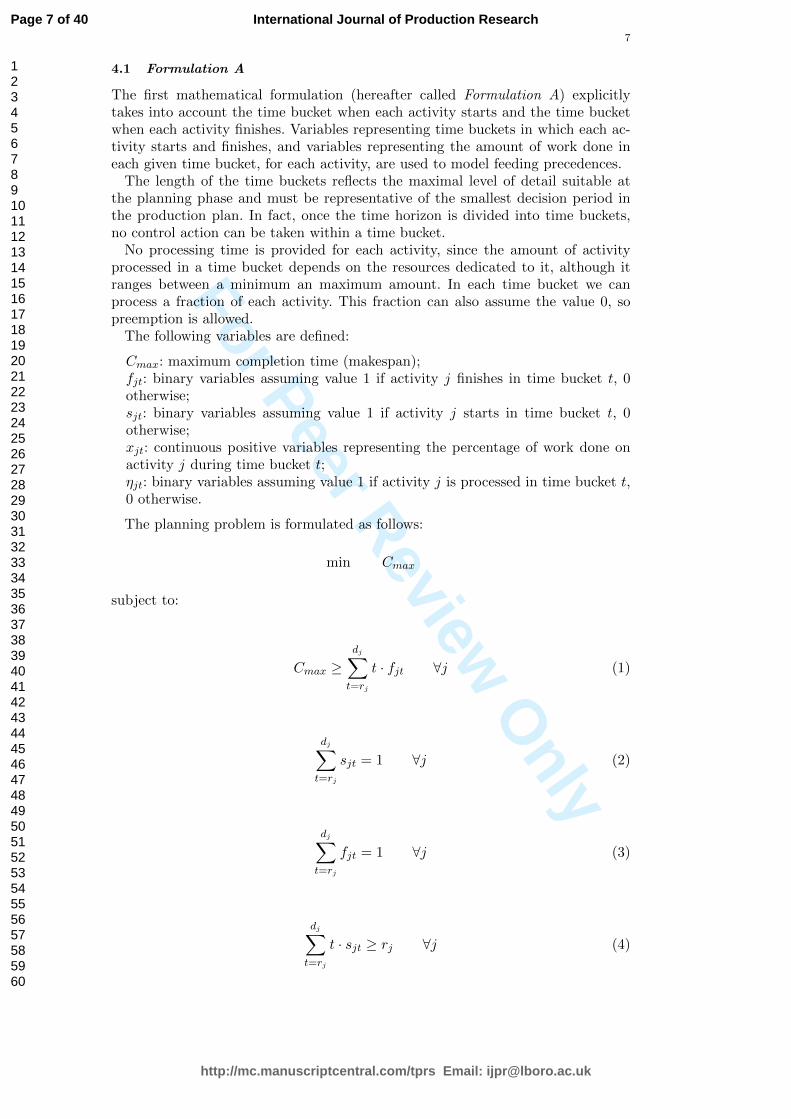
4.1 Formulation A

The first mathematical formulation (hereafter called Formulation A) explicitlytakes into account the time bucket when each activity starts and the time bucketwhen each activity finishes. Variables representing time buckets in which each ac-tivity starts and finishes, and variables representing the amount of work done ineach given time bucket, for each activity, are used to model feeding precedences.

The length of the time buckets reflects the maximal level of detail suitable atthe planning phase and must be representative of the smallest decision period inthe production plan. In fact, once the time horizon is divided into time buckets,no control action can be taken within a time bucket.

No processing time is provided for each activity, since the amount of activityprocessed in a time bucket depends on the resources dedicated to it, although itranges between a minimum an maximum amount. In each time bucket we canprocess a fraction of each activity. This fraction can also assume the value 0, sopreemption is allowed.

The following variables are defined:

Cmax: maximum completion time (makespan);fjt: binary variables assuming value 1 if activity j finishes in time bucket t, 0otherwise;sjt: binary variables assuming value 1 if activity j starts in time bucket t, 0otherwise;xjt: continuous positive variables representing the percentage of work done onactivity j during time bucket t;ηjt: binary variables assuming value 1 if activity j is processed in time bucket t,0 otherwise.

The planning problem is formulated as follows:

min Cmax

subject to:

Cmax ≥dj∑

t=rj

t · fjt ∀j (1)

dj∑t=rj

sjt = 1 ∀j (2)

dj∑t=rj

fjt = 1 ∀j (3)

dj∑t=rj

t · sjt ≥ rj ∀j (4)

Page 7 of 40



123456789101112131415161718192021222324252627282930313233343536373839404142434445464748495051525354555657585960

For Peer Review O

nly

8

dj∑t=rj

xjt = 1 ∀j (5)

xjt ≤ Bjηjt ∀j, t (6)

xjt ≥ bjηjt ∀j, t (7)

sjt ≤ ηjt ∀j, t (8)

fjt ≤ ηjt ∀j, t (9)

fjt ≤t∑

h=rj

xjh ∀j, t (10)

t∑h=rj

sjh ≥ xjt ∀j, t (11)

∑i

Qikxit ≤ Rkt ∀k, t (12)

sjt ≤t−1∑h=1

xih − qp + 1 ∀p ∈ T1, i = ip, j = jp, ∀t (13)

(1−t∑

h=1

fjt) ≥ qp −t−1∑h=1

xih ∀p ∈ T3, i = ip, j = jp, ∀t (14)

t∑h=1

xjh ≤ gp + (1− gp)t−1∑h=1

sih ∀p ∈ T2, i = ip, j = jp, ∀t (15)

t∑h=1

xjh ≤ gp + (1− gp)t−1∑h=1

fih ∀p ∈ T4, i = ip, j = jp, ∀t (16)

Constraint (1) simply defines the makespan as the completion time of the lastcompleted activity. Each activity must have a unique start and a unique finishtime bucket, and these two requirements are assured by constraints (2) and (3),respectively. Moreover, no activity can start before its release date (constraint (4)),

Page 8 of 40



123456789101112131415161718192021222324252627282930313233343536373839404142434445464748495051525354555657585960

For Peer Review O

nly

9

and, in the time horizon between its release date and due date, each activity mustbe completely processed (constraint (5)).

If activity j is processed in time bucket t, the amount of work done on it mustrespect the maximum and minimum thresholds Bj and bj (constraints (6) and (7)).These constraints are mainly due to technological and/or economical reasons, since,depending on the type of activity and on the required resources, it can be infeasibleor non-economical to process an activity more or less than a given amount.

Constraints (8) and (9) forbid an activity to effectively start or finish (s and fequal to 1) in a time bucket where it is not processed (η = 0).

Constraints (10) and (11), on the other hand, represent the obvious fact that anactivity cannot finish if it has not been completed and cannot be processed if is notstarted (i.e., they link the x variables to f and s variables, assuring consistency inthe plan). The total amount of resources used by the activity processing must notexceed, for each resource and in each time bucket, the total amount available inthe time bucket. This is assured by constraint (12).

Constraints (13) to (16) represent the feeding precedences between two activities.Constraint (13) represents the %Completed-to-Start relations. Given a certain timebucket t, for all the %Completed-to-Start precedence relations (p ∈ T1), until thepredecessor activity i = ip has been cumulatively processed for at least a percentageqp, the successor activity j = jp cannot start (sjt < 1). Constraint (15) representsthe Start-to-%Completed precedences. Given a certain time bucket t, for all theStart-to-%Completed precedence relation (p ∈ T2), assures that, the cumulativeexecution of activity j = jp can be greater than percentage gp only if activity

i = ip has started. In fact,∑t

h=1 xjh can be greater than gp only if∑t−1

h=1 sih =1. Constraints (14) and (16) work in a similar way (just substituting start withfinish in the previous descriptions) for the other types of relations. In particular,constraint (14) represents %Completed-to-Finish relations while constraint (16)represents Finish-to-%Completed relations.

4.2 Formulation B

The second mathematical formulation (hereafter called Formulation B) does notexplicitly consider the start time and finish time bucket of the activities. Instead,an execution mask zjt is defined for each activity j. It is possible to process activityj in time bucket t only if the execution mask zjt assumes the value 1. The executionmasks zjt have value 1 at t = 0 and are constrained to have non-increasing shapes.Hence, the mask zjt assumes value 0 only after activity j has been completed, andcan be used to model precedence relations, i.e., that the successor activity can beprocessed only if the execution mask of the predecessor activity has the value 0.Appropriate execution masks zp,t representing feeding precedence are defined foreach precedence relation p.

• %Completed-to-Start and %Completed-to-Finish precedences: the executionmask zp,t associated to these types of precedence relation assumes value 1 whilethe fraction of the predecessor activity i = ip is smaller than qp. When, in timebucket t, the percentage processing of predecessor activity i = ip becomes greaterthan or equal to qp, the execution mask zp,t assumes value 0 for t ≥ t+ 1.

• Start-to-%Completed and Finish-to-%Completed precedences: the executionmask zp,t associated to these types of precedence relation assumes value 1 whilethe processed fraction of the successor activity j = jp is smaller than gp. When,in time bucket t, this fraction becomes greater than or equal to gp, the executionmask zp,t assumes value 0 for t ≥ t+ 1.

Page 9 of 40



123456789101112131415161718192021222324252627282930313233343536373839404142434445464748495051525354555657585960

For Peer Review O

nly

10

In Formulation B, execution masks zjt and zp,t are Boolean variables used tomodel the execution of activities thus playing the roles of the variables sjt and fjtin Formulation A.

min Cmax

subject to:

Cmax ≥ t · zjt ∀j, t (17)

dj∑t=rj

xjt = 1 ∀j (18)

xjt ≤ Bjηjt ∀j, t (19)

xjt ≥ bjηjt ∀j, t (20)

xjt ≤ Bjzjt ∀j, t (21)

zj,t−1 ≥ zjt ∀j, t (22)

∑i

Qjkxjt ≤ Rkt ∀k, t (23)

zp,t−1 ≥ zp,t ∀p ∈ T ,∀t (24)

xjt ≤ Bj(1− zp,t) ∀p ∈ T1, i = ip, j = jp, ∀t (25)

t−1∑h=1

xih ≥ bi − zp,t ∀p ∈ T2, i = ip, j = jp,∀t (26)

(1−t∑

h=1

xjh) ≥ bjzp,t ∀p ∈ T3, i = ip, j = jp,∀t (27)

xit ≤ Bizp,t ∀p ∈ T4, i = ip, j = jp,∀t (28)

Page 10 of 40



123456789101112131415161718192021222324252627282930313233343536373839404142434445464748495051525354555657585960

For Peer Review O

nly

11

t−1∑h=1

xih ≥ qp(1− zp,t) ∀p ∈ (T1 ∪ T3), i = ip,∀t (29)

(1−t∑

h=1

xjh) ≥ (1− gp)zp,t ∀p ∈ (T2 ∪ T4), j = jp,∀t (30)

Constraint (17) defines the makespan as the last possible time bucket when someactivity can still be processed. After it, all masks will be 0 and all activities mustbe completed. Constraints (18), (19) and (20) are identical to constraints (5), (6)and (7) in Formulation A. In particular, constraint (18) assures that each activity jis completely processed within its release date rj and due date dj , while constraints(19) and (20) assure that when xjt is greater than zero (ηjt = 1), i.e., activity j isprocessed in time bucket t, and the percentage of activity j processed in time buckett is greater than the minimum amount bj but does not exceed the maximum amountBj . These constraints avoid the fragmentation of each activity execution, whilerespecting economic and feasibility criteria. The resource constrains are assured by(23).

Constraint (21) defines the z variables assuring that an activity can be processed(i.e., xjt > 0) only if its execution mask zjt assumes value 1. Constraint (24) assuresthat the execution masks are non-increasing functions of t while constraints (25)-(30) model feeding precedences. In particular, constraints (25) to (28) define thedifferent type of precedence relations using the execution masks zp,t, while thebehavior of the execution mask zp,t is controlled by constraints (29)-(30).

Figure 5

The definition of the execution masks for feeding precedences depends on the typeof the precedence relation. For %Completed-to-Start and %Completed-to-Finishprecedence relations (p ∈ (T1∪T3)), the execution mask is associated to the prede-cessor activity i = ip: while the executed fraction of the predecessor activity is lessthan qp, the mask must have value 1. When the executed fraction is greater thanqp the mask can assume either value 1 or 0 (Figure 5(a) and 5(c)). This behavior isdefined by the constraint (29). The execution mask constrains the execution of thesuccessor activity j = jp. For %Completed-to-Start precedence relations, constraint(25) prevents the successor activity j = jp from starting if the value of the mask is 1(xjt can not > 0). For %Completed-to-Finish precedence relations, constraint (27)assures that, until the mask assumes the value 1, the successor activity can not becompleted. Hence, when the mask assumes the value 0, the successors j = jp shouldhave completed at least a fraction bj , that is, the minimum fraction processable ina single time bucket.

When Start-to-%Completed and Finish-to-%Completed precedence relations areconsidered, on the other hand, the execution mask refers to the successor activityj = jp. In these cases, constraint (30) forces the execution mask zp,t to assumevalue 0 as soon as the executed fraction of the successor activity j = jp reachesgp (Figure 5(b) and 5(d)). For the Start-to-%Completed relations, constraint (26)assures that, if the execution mask assumes value 0, then the executed fraction ofthe predecessor activity i = ip must be at least bi. Since bi is the minimum fractionprocessable in a single time bucket, then the predecessor activity should at least bestarted. For Finish-to-%Completed relations, constraint (28) imposes that, whenthe execution mask assumes the value 0, it is no longer possible to process thepredecessor activity i = ip (xit ≤ 0); hence, this activity should already have been

Page 11 of 40



123456789101112131415161718192021222324252627282930313233343536373839404142434445464748495051525354555657585960

For Peer Review O

nly

12

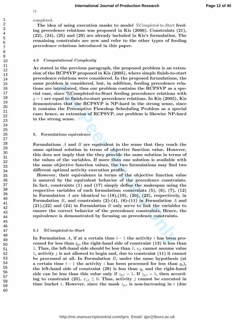
completed.The idea of using execution masks to model %Completed-to-Start feed-

ing precedence relations was proposed in Kis (2006). Constraints (21),(22), (24), (25) and (29) are already included in Kis’s formulation. Theremaining constraints are new and refer to the other types of feedingprecedence relations introduced in this paper.

4.3 Computational Complexity

As stated in the previous paragraph, the proposed problem is an exten-sion of the RCPSVP proposed in Kis (2005), where simple finish-to-startprecedence relations were considered. In the proposed formulations, thesame problem is considered, but, in addition, feeding precedence rela-tions are introduced, thus our problem contains the RCPSVP as a spe-cial case, since %Completed-to-Start feeding precedence relations withq = 1 are equal to finish-to-start precedence relations. In Kis (2005), Kisdemonstrates that the RCPSVP is NP-hard in the strong sense, sinceit contains the Preemptive Flowshop Scheduling Problem as a specialcase; hence, as extension of RCPSVP, our problem is likewise NP-hardin the strong sense.

5. Formulations equivalence

Formulations A and B are equivalent in the sense that they reach thesame optimal solution in terms of objective function value. However,this does not imply that the they provide the same solution in terms ofthe values of the variables. If more than one solution is available withthe same objective function values, the two formulations may find twodifferent optimal activity execution profile.

However, their equivalence in terms of the objective function valueis assured by the equivalent behavior of the precedence constraints.In fact, constraints (1) and (17) simply define the makespan using therespective variables of each formulation; constraints (5), (6), (7), (12)in Formulation A are identical to (18),(19), (20), (23), respectively, inFormulation B, and constraints (2)-(4), (8)-(11) in Formulation A and(21),(22) and (24) in Formulation B only serve to link the variables toensure the correct behavior of the precedence constraints. Hence, theequivalence is demonstrated by focusing on precedence constraints.

5.1 %Completed-to-Start

In Formulation A, if at a certain time t − 1 the activity i has been pro-cessed for less than qp, the right-hand side of constraint (13) is less than1. Thus, the left-hand side should be less than 1, sjt cannot assume value1, activity j is not allowed to begin and, due to constraint (11) it cannotbe processed at all. In Formulation B, under the same hypothesis (ata certain time t − 1 the activity i has been processed for less than qp),the left-hand side of constraint (29) is less than qp and the right-handside can be less than this value only if zp,t = 1. If zp,t = 1, then accord-ing to constraint (25), xj,t ≤ 0. Thus, activity j cannot be executed intime bucket t. However, since the mask zp,t is non-increasing in t (due

Page 12 of 40



123456789101112131415161718192021222324252627282930313233343536373839404142434445464748495051525354555657585960

For Peer Review O

nly

13

to constraint (24)), it must assume the value 1 in all the time bucketsbefore t, so activity j cannot be executed before t and, consequently, itcan not begin.

If, on the other hand, at a certain time t − 1, activity i has beenprocessed for more than qp, the right-hand side of constraint (13) inFormulation A is greater than or equal to 1. In this case sjt is no longerconstrained (sjt ∈ [0, 1]) and activity j can begin. In Formulation B, underthe same hypothesis, constraint (29) allows zp,t to assume either value 0or 1. Thus, according to (25), 0 ≤ xjt ≤ bj and activity j can begin in t.

5.2 Start-to-%Completed

If, at a certain time t − 1, activity i has not begun, the right-hand sideof constraint (15) in Formulation A assumes the value gp and the left-hand side (fraction of activity j executed) cannot be greater than thisvalue. Under the same hypothesis, in Formulation B, the left-hand-sideof constraint (26) assumes value 0 (activity i has not begun). Constraint(26) thus forces the value of zp,t to be 1. Therefore, the right-hand sideof the constraint (30) assumes the value 1−gp. To satisfy constraint (30),the left-hand side must not be less than 1− gp and hence the fraction ofactivity j processed until time bucket t cannot be greater than gp.

If, on the other hand, at a certain time t − 1, activity i has alreadybegun, the right-hand side of constraint (15) in Formulation A assumesthe value 1 and the left-hand side is no longer constrained. Hence, theprocessed fraction of activity j can be greater than gp. In FormulationB, if activity i has already begun, it must be processed for at leas afraction bj. Due to constraint (26), zp,t is allowed to assume the value 0.Considering the constraint (30), if zp,t is allowed to assume the value 0,then the value of the right-hand side can be also 0, and the left-handside is no longer constrained, so the fraction of activity j processed untiltime bucket t can be greater than gp.

5.3 %Completed-to-Finish

In Formulation A, constraint (14) assures that, if at a certain time t− 1,activity i has been processed for less than qp, then the right-hand sideof the constraint is greater than 0. Then, the left-hand side should alsobe greater than 0; hence fjt cannot assume the value 1, i.e., activity jis not allowed to finish (according to constraint(10)). Under the samehypothesis, in Formulation B, the left-hand side of constraint (29) mustbe less than qp and hence zp,t is constrained to assume the value 1.Therefore, the right-hand side of constraint (27) assumes the value bj.Since the left-hand side of constraint (27) represents the fraction ofactivity j not yet processed, and this fraction should be greater than bj,activity j cannot be completed.

If, on the other hand, at a certain time t − 1 activity i has been pro-cessed for more than qp, the right-hand side of constraint (14), in For-mulation A, is less than 0, so the left side is no longer constrained, fjtcan assume the value 1, and hence, activity j can be completed. Underthe same hypothesis, in Formulation B, the right-hand side of constraint(29) is greater or equal to qp and zp,t is allowed to assume the value 0. Ifzp,t can assume value the 0, then the right-hand side of constraint (27)

Page 13 of 40



123456789101112131415161718192021222324252627282930313233343536373839404142434445464748495051525354555657585960

For Peer Review O

nly

14

can be 0, i.e., the fraction of activity j not yet processed can be 0, andhence, activity j can be completed.

5.4 Finish-to-%Completed

If, at a certain time t − 1, activity i has not been completed, then theright-hand side of constraint (16), in Formulation A, assumes the valuegp, and hence the fraction of activity j executed cannot be greater thanthis value. Under the same hypothesis, in Formulation B, the value of zp,tin constraint (30) must be 1, implying that activity j cannot be executedfor a percentage greater than gp. In fact, it is possible to process activity i(i.e., xit > 0) only if the value of zp,t is 1 in constraint (28). Since the maskzp,t is non-increasing (as stated by constraint (24)) in t, until activity ihas not be finished, zp,t must be 1; otherwise it is not possible to processi anymore. Hence, activity i cannot be finished.

If, on the other hand, at a certain time t − 1, activity i has beencompleted, then the right-hand side of constraint (16), in FormulationA, assumes the value 1 and the left-hand side is no longer constrained.Hence the fraction of activity j processed can be greater than gp. InFormulation B, if activity i has already been completed, then zp,t canassume the value 0. If zp,t can assume the value 0, then the right-hand sideof constraint (30) is no longer constrained and the fraction of activity jprocessed until time bucket t can be greater than gp.

6. On the definition of the feeding precedence relations

The feeding precedence relations described above can sometimes demon-strate somewhat pathological behavior. When %Completed-to-Finishprecedence relations are used, both mathematical formulations allow ahigh percentage of the successor activity j to be executed (e.g., 99.99%)and then wait until qij of the predecessor activity i has been executedto finish j. In the case of Start-to-%Completed, activity i can start andbe processed for only for a very small percentage (e.g., 0.01%) to al-low activity j to be completed for more than gij. Although possible,such pathological behaviors can be avoided through an appropriate cal-ibration of the parameters bj, together with a proper structure of theprecedence relations among the aggregate activities.

In fact, bj can be used to model work organization (a single workercannot work alone) or technological issues (if an activity is executed ina time bucket, then a minimum amount of working hours should be de-voted to it) thus making the probability of processing an activity for aextremely small fraction quite unlikely. The mathematical formulationsalso allow us to define more than one precedence relation between thesame pair of activities. This can be used to shape the mutual execu-tion of a pair of activities to assure compatibility with the reality. Asan example, it can be stated that successor j can start only when thepercentage executed of i is ≥ q, but, at the same time, the executionof activity i can be more than g only if activity j has already started(Figure 6).

Figure 6

Page 14 of 40



123456789101112131415161718192021222324252627282930313233343536373839404142434445464748495051525354555657585960

For Peer Review O

nly

15

7. Morphological and resource-related issues

A project scheduling problem can be represented by means of an acyclic directedgraph G = V,U using an activity-on-node representation. Each activity is repre-sented by a node in the set V while each arc in the set G represents a precedenceconstraint between two activities. It is common practice, in the project schedulingliterature, to characterize a problem through morphological and resource-relatedmeasures of its graph representation. In (Tavares et al. 1999, Vanhoucke et al. 2004)several complexity measures are proposed to describe the morphological structureof a network while in (Demeulemeester et al. 2003) resource-related measures arepresented. Some of the morphological and resource-related measures considered inthe above cited papers are briefly described in the following, as they will be usedin Section 8 to characterize the complexity of the networks we experimented with.

Among the morphological indices presented in (Tavares et al. 1999, Vanhouckeet al. 2004), we consider the following:

• I1: Size of the Problem. This index is equal to the number of nodes (i.e., activities)in the network and it is a measure of the size of the network.

• I2: Serial or Parallel Indicator. It measures how close a network is to a serial orparallel directed graph. When all activities are in parallel, I2 = 0, while whenall the activities are serially connected, I2 = 1. Real networks contain a numberof activities that can be executed in parallel and a number of serial precedences:the closer to 1 is the value of I2, the larger the number of serial connections withrespect to the parallel components of the network.

Among the resource-related measures presented in (Demeulemeester et al. 2003),we consider:

• RU : Resource density. RU measures, for each activity, the number of resourcesit uses (not the quantity used). The value of this index varies between 0, if theactivity needs no resource, to the maximum number of resources available, if theactivity uses all the available resources. RU can only assume integer values.

• RC: Resource constrainedness. It computes, for each resource, the ratio betweenthe average quantity (over all activities that use the resource) required for theresource and its total availability. RC is zero if no activity uses the resource, whileit approaches 1 if all activities, requiring the resource, demand for a quantityclose to the total availability. If RC is bigger than 1, the problem is resource-infeasible, since, on average, more of the resource is required than the availablequantity.

In Section 8, the performance of Formulations A and B are tested on randomgenerated instances and on an industrial case. In the following comparison, 1)the random instances were generated by fixing the above described morphologicaland resource-related indices so that they well represent industrial problems typicalof the system we are considering (Manufacturing-to-Order and Engineering-to-Order), but with significant differences among the various classes of instances, and2) the industrial case instances were classified according to the morphological andthe resource aspects of the activity network.

8. Computational experiments

The two mathematical formulations presented in Section 4 were tested using bothrandom generated instances and instances drawn from an industrial application.The two mathematical formulations were solved by using CPLEX 10.0 on a XEON

Page 15 of 40



123456789101112131415161718192021222324252627282930313233343536373839404142434445464748495051525354555657585960

For Peer Review O

nly

16

workstation (clock: 3.0 Ghz, RAM: 4.00 Gb). A preliminary computational testwas carried out to investigate the possible influence of the CPLEX settings (inparticular the generation of different type of cuts) on the solution time. The resultsshowed no particular effect of such settings on the solution time; moreover, thesolution time obtained with the standard settings of CPLEX was always amongthe best ones. Hence, we experimented with the standard CPLEX settings, sincethe solution time with standard settings can be considered a strong indication ofthe difficulty of solving the instances.

8.1 Random generated instances

The random instances were generated using RanGen2 (Vanhoucke et al. 2008),an activity network instance generator for project scheduling problems based onthe indicators described in the previous section. RanGen2, however, generates in-stances for classical resource constrained project scheduling problem, i.e., instanceswith fixed activity durations and finish-to-start precedence relations. To use vari-able intensity formulation for activity execution and feeding precedences betweenactivities, the generated instances were modified in the following way:

• A given fraction of finish-to-start precedence relations is randomly chosen andtransformed to feeding precedences with 50% overlap (i.e., qij and gij are equalto 0.5).

• The duration Lj of activity j is considered as the minimum duration, i.e., Bj =1/Lj . The minimum fraction of activity processable in each time bucket is notconstrained (bj = 0).

A set of problem instances were generated using the generation parameters re-ported in Table 1. The roles of I1, I2, RU and RC are as described in the previoussection, and Res indicates the number of resources in each instance.

Table 1

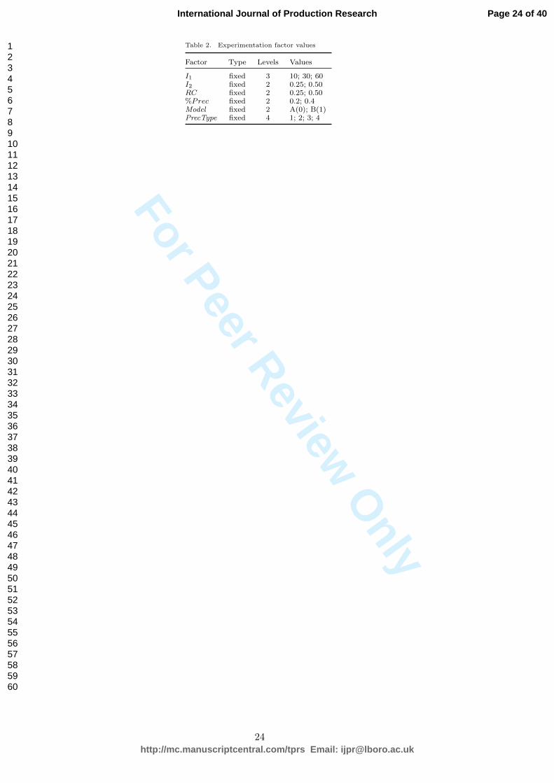
For each combination of the values for I1, I2, Res, RU and RC in Table 1, 2000instances were generated. Then, to assure the complete randomness of the testinstances, for each class of instances, a set of 100 instances was sampled to be usedfor the experiments. Given an instance, a certain percentage %Prec of the existingprecedence relations are changed to feeding precedence relations of the same typePrecType. Different types of feeding precedences are tested in a separate way, i.e.,in each experiment, only one type of feeding precedence is considered (besidesthe usual finish-to-start). The feeding precedence relation types are coded as 1(CtS), 2 (CtF), 3 (StC) and 4 (FtC). Then the mathematical formulations A andB (Model) are used to solve the instances. The factors used in the computationaltests are reported in Table 2.

Table 2

8.2 Results

In the experimental tests, a maximum solution time of 1000 seconds was set foreach experiment. If it is not solved to optimality within 1000 seconds, an exper-iment is considered a failure. Given the dimension of the instances, 1000 secondscan be considered a suitable threshold to identify failures in the solution of the in-stances. The result summary (Table 3) reports the average solution time (AvTime)and the percentage of failures (PercFail) in solving the instance to optimality given

Page 16 of 40



123456789101112131415161718192021222324252627282930313233343536373839404142434445464748495051525354555657585960

For Peer Review O

nly

17

the number of activities (I1) and the formulation (Model).The results show that, as expected, the solution time increases with the number ofactivities. The behavior of the two formulations is however quite different. Formu-lation A has a significantly longer solution time, and hence, a larger percentage offailures than formulation B.

Table 3

Given the considerable influence of the number of activities and the mathemat-ical formulation on the performance, both in terms of the solution time and thepercentage of failures (Table 3), we investigated the joint influence of all the pa-rameters used to generate instances has been investigated.

A first analysis was carried out to analyze the influence of the generation param-eters on the percentage of failures. A preliminary qualitative analysis is reportedin Figure 7. This confirms that the main factors influencing the number of failuresare the number of activities (I1), the mathematical formulation used (Model) andthe the shape of the activity network (I2). In addition, the value of RC has a slightinfluence, causing the problem to be more difficult to solve as the RC value in-creases. The remaining factors (the amount and type of feeding precedences, %Precand PrecType), on the other hand, did not show any significant influence.

To complete the analysis, the interaction between pairs of factors is investigatedthrough the Interaction Plot shown in Figure 8. The graph shows a clear interac-tion between the number of activities (I1) and the formulation used (Model). Inparticular, Formulation A is strongly influenced by the value of I1 (for 60 activi-ties, the percentage of failure is consistent) while when Formulation B is used, theinfluence of (I1) is significantly less.

Figure 7

Figure 8

A second analysis is carried out to investigate the influence of the generationparameters on the time needed to solve a problem to optimality. Clearly, in thisanalysis, only the experiments that did “not fail” (i.e., for which it was possible toreach optimality within 1000 seconds) were considered.

The graph of the main effects (Figure 9) confirms that the influencing factors are,also for the solution time, the dimension of the problem (I1) and the mathematicalformulation (Model). The resources load (RC) has a slightly greater influence whilethe type of precedence relations (PrecType) shows an interesting pattern: test caseswith precedence type 2 seems less difficult to solve than those of types 1, 3 and 4.

The analysis of the interactions between factors (Figure 10) indicates that thedimension of the problem (I1) magnifies the effects of all the other factors. Infact, when I1 = 60 the influence of RC, %Prec and PrecType is more evident.However, when the formulation B is used (Model = 1) the influence of I1 is stronglydecreased. The influence of feeding precedence type (PrecType) shows the samepattern seen in the Main Effect Plot (Figure 9), i.e., the solution time for problemswith only feeding precedences of type 2 is shorter than for the other types ofprecedence relations. This behavior has interaction with I1, RC and Model. Moreprecisely, it becomes most evident when I1 = 60, RC = 0.5 and Formulation A isused (Model = 0).

Figure 9

Figure 10

Page 17 of 40



123456789101112131415161718192021222324252627282930313233343536373839404142434445464748495051525354555657585960

For Peer Review O

nly

18

This influence can be better observed in Table 4, where the average solutiontime and the average percentage of failures are reported, for only the experimentsemploying Formulation A, according to the number of activities in the problem(I1) and the type of precedence relation used (PrecType).

Table 4

In all the experiments, both formulations gave the same results in terms ofmakespan. However, the computational tests on the randomly generated instancesprovide a clear picture of the performance of the two proposed formulations insolving instances with different characteristics. In particular, it can be argued thatthe performance of Formulation A is strongly influenced by the number of activitiesin the scheduling problem, both for the number of failures and the solution time.Formulation B, instead, was able to solve to optimality the vast majority of theinstances in a reasonable time. Moreover, the analysis shows that, when Formula-tion B is used, the number of activities in the instances has almost no influenceon the solution time, thus demonstrating that Formulation B also outperformsFormulation A in terms of robustness.

The results obtained with the two formulations have also been compared interms of solution structure, i.e., how many pieces an activity is preempted onaverage and what percentage is processed in each time bucket. The two formulationsshowed, on average, the same number of preemptions, but while Formulation Atends to preempt less as the processing approaches the due date, Formulation Btends to preempt more evenly. Moreover, Formulation A splits activities in sucha way that the percentage processed in each time bucket (whether the activityis preempted or not) is always the same. For example, if an activity uses 6 timebuckets, 1/6 of it will be processed in each. On the other hand, the solutionsfound by Formulation B also processed different percentages in the time bucketsused (e.g., 6 time buckets used, processed percentages equal to 0.1, 0.2, 0.2, 0.2, 0.1,0.2). These characteristic makes Formulation A more suitable for ad-hoc algorithmsbased on column generation techniques (dynamic programming can be more easilyused to find solutions, in terms of the values of x).

8.3 Industrial application

To demonstrate the viability of the developed method, it was applied to productionplanning in a real industrial environment that produces machining centers. A ma-chining center is a CNC (Computer Numerical Controlled) machine integrated withan automatic tool changer, and it often has equipment for pallet or part handling.

Even if standard machining centers are available, customers often ask for mod-ifications tailored to their specific needs. This is a common practice for European(and in particular Italian) machining center manufacturers. After the customizedparts have been completely designed, a large set of components is assigned toexternal suppliers, while only high precision manufacturing activities for criticalcomponents are executed internally. At the end, all the parts and ancillary compo-nents are assembled together, tested and then partially disassembled and deliveredto the customer.

To model the production process, the bill of materials of a set of machining cen-ter types has been analyzed. Components were grouped into functional units and,for each group, a manufacturing or assembling operation has been considered. Thework content was estimated for each operation, and proper precedence constraintswere defined among them to represent the technological constraints affecting theproduction process. Hence, considering the resources involved, the operations have

Page 18 of 40



123456789101112131415161718192021222324252627282930313233343536373839404142434445464748495051525354555657585960

For Peer Review O

nly

19

been grouped to obtain a reduced set of aggregate production activities: Struc-ture Preparation, Structure Painting, Assembling Autonomous Components, As-sembling, Wiring, Testing, Metrological Testing, Disassembling and Delivery.

Given the aggregate production activities, feeding precedence constraints wereused to model the production process correctly. The need of feeding precedencerelations is motivated by the fact that finish-to-start precedence relations amongaggregate activities impose unnecessary constraints with respect to the real man-ufacturing process.

In fact, the Assembling phase contains a certain number of sub-phases dealingwith the separate assembling of single autonomous components such as the elec-trical cabinet or the spindle head. The assembling of such components need notbe completely processed before the machine assembling activity starts. Rather, itis desirable that these activities be completed at the latest before the subassem-bly is installed onto the machining center (Figure 11). In such a case, a Finish-to-%Completed precedence constraint can be used to allow the assembling of differentautonomous components to be completed at the latest after a certain percentage ofthe machining center assembling has been executed. This percentage represents thepercentage of the assembling activity that can be carried out even if the consideredsubassembly is not yet ready to be installed in the machining center. In a similarway, the wiring and testing phases should not wait for the completion of the wholeassembling phase to start. The wiring phase can start as soon as components thahneed to be wired together are installed in the machining center. furthermore, inthis case, a suitable approach to allow the wiring activity to start at the earliestafter a certain percentage of the assembling activity has been completed. Hence a%Completed-to-Start precedence constraint can be used to allow the cabling phaseto start as soon as the components that need to be cabled together are installedonto the machining center.

Figure 11

Formulations A and B were tested to plan the production of a subset of theproduction orders, drawn from the industrial case, with the objective of minimizingthe total duration of the production activities (i.e., the makespan). The machiningcenters to produce, corresponding to the selected production orders, have the samenumber of activities and the same structure of precedence relations. They differ interms of processing times and percentages used in feeding precedence relations (qijand gij).

For each machining center, three feeding precedence relations are used tocorrectly represent the production process: a Finish-to-%Completed betweenthe Assembling Autonomous Components and the Assembling phases, and two%Completed-to-Start between the Assembling and Wiring and the Assembling andTesting phases. Given the detailed precedence constraints structure between pro-duction operations, the percentages to be used in the feeding precedence relationshave been calculated, for each machining center type, according to the proceduredescribed in Figures 3 and 4. The value of gij for the Finish-to-%Completed prece-dence ranges between 0.21 and 0.25 while the values of qij for the %Completed-to-Start precedences range between 0.65 and 0.78 according to the different types ofmachining centers.

All the described production phases are mainly processed by human workers.Their behavior can be correctly modeled using the variable intensity formulationallowing a variable resource utilization. The workers are grouped into seven differ-ent types according to their particular skills (Res = 7) and each production phaserequires only one type of workers (RU = 1).

Page 19 of 40



123456789101112131415161718192021222324252627282930313233343536373839404142434445464748495051525354555657585960

For Peer Review O

nly

20

The value of RC in the randomly generated instances considered a constantavailability of resources. In the industrial case, however, this hypothesis does nothold. In fact, the availability of resources depends on the request of the other ordersnot considered in the experiments. The value for RC has therefore been calculatedthrough an average availability over the time horizon considered. Moreover, as de-scribed in Section 7, the value of RC depends on the amount of resources requestedby all the activities. In the considered industrial case, the amount of resources re-quested depends on the type of machining centers to be produced. Hence, differentvalues for RC are obtained for the different industrial instances considered.

In Table 5, the values of the parameters characterizing the industrial case arereported. Notice that, in contrast to the randomly generated instances, the differenttypes of feeding precedence relations are mixed together in the same instance.Notice also that, since the parameters were directly derived from the industrialdata, there is no discretion about them. For this reason, we did not investigatethe sensitivity of the results to the parameter values, as we did for the randomgenerated instances.

Table 5

In Table 6 the results of the experiments on the industrial case are reported.It can be observed that, for each instance, the solution times are smaller whenFormulation B is used. Moreover, in two instances (IC1 and IC2 ), Formulation Afailed, i.e., it was not able to solve the problem to optimality within the time limitof 1000 seconds. Considering only the successful cases, Formulation A was solvedto optimality in an average time of 6.78 seconds while the average solution timefor Formulation B was 2.55 seconds. These results are in line with those obtainedusing the randomly generated instances.

Table 6

9. Conclusion and further research

This paper has addressed the problem of production planning in Manufacturing-to-Order or Engineering-to-Order systems producing complex and highly customizeditems. A project scheduling approach has been proposed using variable intensityformulations to allow the effort committed to the execution of activities to vary overtime. Feeding precedence relations were developed to model generalized precedencerelations when the execution mode of activities is not known a priori and theirpossible utilizations have been described through the application to a real industrialcase.

Two alternative mathematical formulations were proposed and tested on ran-domly generated instances and on real instances drawn from an industrial case inorder to show the application of the approach. The results of the computationaltests, both on randomly generated and industrial instances, highlighted the dif-ferent performance levels and the main characteristics of the two mathematicalformulations. In particular, the tests allowed us to evaluate their different levels ofsensitivity to the parameters defining the characteristics of the production planningproblem, such as the number of activities and the load of the resources.

The computational experiments were carried out using a commercial software(Ilog CPLEX) to solve the mathematical formulations. The use of a commercialsoftware might reduce the effort required to introduce the proposed approach to afirm. However, the numerical results clearly showed that this is a viable approachonly with small instances. In fact, the use of commercial software might be im-

Page 20 of 40



123456789101112131415161718192021222324252627282930313233343536373839404142434445464748495051525354555657585960

For Peer Review O

nly

REFERENCES 21

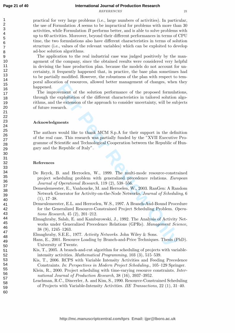
practical for very large problems (i.e., large numbers of activities). In particular,the use of Formulation A seems to be impractical for problems with more than 30activities, while Formulation B performs better, and is able to solve problems withup to 60 activities. Moreover, beyond their different performances in terms of CPUtime, the two formulations also have different characteristics in terms of solutionstructure (i.e., values of the relevant variables) which can be exploited to developad-hoc solution algorithms.

The application to the real industrial case was judged positively by the man-agement of the company, since the obtained results were considered very helpfulin devising the base production plan. because the models do not account for un-certainty, it frequently happened that, in practice, the base plan sometimes hadto be partially modified. However, the robustness of the plan with respect to tem-poral allocation of resources, allowed better management of changes, when theyhappened.

The improvement of the solution performance of the proposed formulations,through the exploitation of the different characteristics in tailored solution algo-rithms, and the extension of the approach to consider uncertainty, will be subjectsof future research.

Acknowledgments

The authors would like to thank MCM S.p.A for their support in the definitionof the real case. This research was partially funded by the ”XVII Executive Pro-gramme of Scientific and Technological Cooperation between the Republic of Hun-gary and the Republic of Italy”.

References

De Reyck, B. and Herroelen, W., 1999. The multi-mode resource-constrainedproject scheduling problem with generalized precedence relations. EuropeanJournal of Operational Research, 119 (2), 538–556.

Demeulemeester, E., Vanhoucke, M. and Herroelen, W., 2003. RanGen: A RandomNetwork Generator for Activity-on-the-Node Networks. Journal of Scheduling, 6(1), 17–38.

Demeulemeester, E.L. and Herroelen, W.S., 1997. A Branch-And-Bound Procedurefor the Generalized Resource-Constrained Project Scheduling Problem. Opera-tions Research, 45 (2), 201–212.

Elmaghraby, Salah, E. and Kamburowski, J., 1992. The Analysis of Activity Net-works under Generalized Precedence Relations (GPRs). Management Science,38 (9), 1245–1263.

Elmaghraby, S.E.E., 1977. Activity Networks. John Wiley & Sons.Hans, E., 2001. Resource Loading by Branch-and-Price Techniques. Thesis (PhD).

University of Twente.Kis, T., 2005. A branch-and-cut algorithm for scheduling of projects with variable-

intensity activities. Mathematical Programming, 103 (3), 515–539.Kis, T., 2006. RCPS with Variable Intensity Activities and Feeding Precedence

Constraints. In: Perspectives in Modern Project Scheduling., 105–129 Springer.Klein, R., 2000. Project scheduling with time-varying resource constraints. Inter-

national Journal of Production Research, 38 (16), 3937–3952.Leachman, R.C., Dincerler, A. and Kim, S., 1990. Resource-Constrained Scheduling

of Projects with Variable-Intensity Activities. IIE Transactions, 22 (1), 31–40.

Page 21 of 40



123456789101112131415161718192021222324252627282930313233343536373839404142434445464748495051525354555657585960

For Peer Review O

nly

22 REFERENCES

Markus, A., Vancza, J., Kis, T. and Kovacs, A., 2003. Project scheduling approachfor production planning. Annals of the CIRP, 52 (1), 359–362.

Neumann, K. and Schwindt, C., 1998. A capacitated hierarchical approach to make-to-order production. European Journal of Automation, 32, 397–413.

Neumann, K., Schwindt, C. and Zimmermann, J., 2003. Project scheduling withtime windows and scarce resources - temporal resource-constrained projectscheduling with regular and nonregular objective functions. 2nd ed. SpringerBerlin.

Neumann, K. and Schwindt, C., 1997. Activity-on-node networks with minimaland maximal time lags and their application to make-to-order production. ORSpectrum, 19 (3), 205–217.

Tavares, L.V., Ferreira, J.A. and Coelho, J.S., 1999. The risk of delay of a projectin terms of the morphology of its network. European Journal of OperationalResearch, 119 (2), 510–537.

Tolio, T. and Urgo, M., 2007. Planning of Machining Centres Production: the Roleof Precedence Modelling. Montecatini, Italy, 10 – 12 September 2007.

Vancza, J., Kis, T. and Kovacs, A., 2004. Aggregation: the Key to IntegratingProduction Planning and Scheduling. Annals of the CIRP, 53 (1), 374–376.

Vanhoucke, M., Coelho, J., Debels, D. and Tavares, L.V., On the morphologicalstructure of a network. , 2004. , Technical report 9, Vlerick Leuven Gent Man-agement School.

Vanhoucke, M., Coelho, J., Debels, D., Maenhout, B. and Tavares, L.V., 2008. Anevaluation of the adequacy of project network generators with systematicallysampled networks. European Journal of Operational Research, 187 (2), 511–524.

Zijm, W.H.M., 2000. Towards intelligent manufacturing planning and control sys-tems. OR Spektrum, 22, 313–345.

Page 22 of 40



123456789101112131415161718192021222324252627282930313233343536373839404142434445464748495051525354555657585960

For Peer Review O

nly

Table 1. Parameter values

for instance generation

I1 10 30 60I2 0.25 0.50Res 4RU 1RC 0.25 0.50

23

Page 23 of 40



123456789101112131415161718192021222324252627282930313233343536373839404142434445464748495051525354555657585960

For Peer Review O

nly

Table 2. Experimentation factor values

Factor Type Levels Values

I1 fixed 3 10; 30; 60I2 fixed 2 0.25; 0.50RC fixed 2 0.25; 0.50%Prec fixed 2 0.2; 0.4Model fixed 2 A(0); B(1)PrecType fixed 4 1; 2; 3; 4

24

Page 24 of 40



123456789101112131415161718192021222324252627282930313233343536373839404142434445464748495051525354555657585960

For Peer Review O

nly

Table 3. Average aggregate results

I1 Model AvTime % Failures Model AvTime % Failures

10 A 1.7023 0.12 B 0.1779 0.00%30 A 115.1464 16.88 B 5.8271 1.94%60 A 255.0025 93.38 B 56.7425 12.19%

25

Page 25 of 40



123456789101112131415161718192021222324252627282930313233343536373839404142434445464748495051525354555657585960

For Peer Review O

nly

Table 4. Influence of precedence type for instances of

Formulation A

I1 PrecType Average Time % Failures

10 1 2.79 0.00%10 2 0.86 0.25%10 3 1.82 0.00%10 4 1.33 0.25%30 1 151.19 13.00%30 2 69.19 11.00%30 3 106.73 11.50%30 4 140.14 32.00%60 1 262.22 94.75%60 2 187.79 91.50%60 3 261.62 89.50%60 4 461.20 97.75%

26

Page 26 of 40



123456789101112131415161718192021222324252627282930313233343536373839404142434445464748495051525354555657585960

For Peer Review O

nly

Table 5. Industrial case pa-

rameters

Parameters Values

I1 30I2 0.22RC (0.13,0.19)%Prec 0.25Model A(0); B(1)PrecType mixed

27

Page 27 of 40



123456789101112131415161718192021222324252627282930313233343536373839404142434445464748495051525354555657585960

For Peer Review O

nly

Table 6. Industrial case results

Instance I1 I2 RC %Prec Model T ime Model T ime

IC1 30 0.222 0.18849 0.25 A – B 9.73IC2 30 0.222 0.18808 0.25 A – B 7.69IC3 30 0.222 0.1654 0.25 A 10.05 B 1.05IC4 30 0.222 0.15207 0.25 A 7.08 B 1.19IC5 30 0.222 0.17784 0.25 A 9.97 B 1.00IC6 30 0.222 0.15207 0.25 A 6.52 B 1.11IC7 30 0.222 0.16363 0.25 A 5.08 B 0.95IC8 30 0.222 0.15538 0.25 A 4.39 B 1.25IC9 30 0.222 0.13906 0.25 A 2.66 B 0.75IC10 30 0.222 0.15538 0.25 A 8.55 B 0.80

28

Page 28 of 40



123456789101112131415161718192021222324252627282930313233343536373839404142434445464748495051525354555657585960

For Peer Review O

nly

Figure 1. Generalized precedence relations with time lags.

Figure 2. Feeding precedence relations.

Figure 3. Aggregation of activities.

Figure 4. Feeding precedence on aggregate activities.

Figure 5. Execution masks for feeding precedence relations.

Figure 6. Multiple precedence constraints.

Figure 7. Main Effects Plot for mean failures percentage.

Figure 8. Interaction Plot for mean failures percentage.

Figure 9. Main Effects Plot for mean solution time.

Figure 10. Interaction Plot for mean solution time.

Figure 11. Machining Center structure with preassembled components installed.

29

Page 29 of 40



123456789101112131415161718192021222324252627282930313233343536373839404142434445464748495051525354555657585960

For Peer Review O

nly

Figure 1. Generalized precedence relations with time lags. 180x68mm (72 x 72 DPI)

Page 30 of 40



123456789101112131415161718192021222324252627282930313233343536373839404142434445464748495051525354555657585960

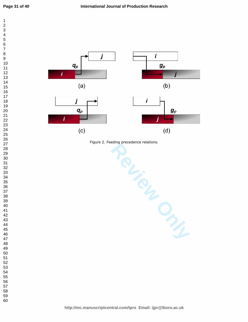
For Peer Review O

nly

Figure 2. Feeding precedence relations.

Page 31 of 40



123456789101112131415161718192021222324252627282930313233343536373839404142434445464748495051525354555657585960

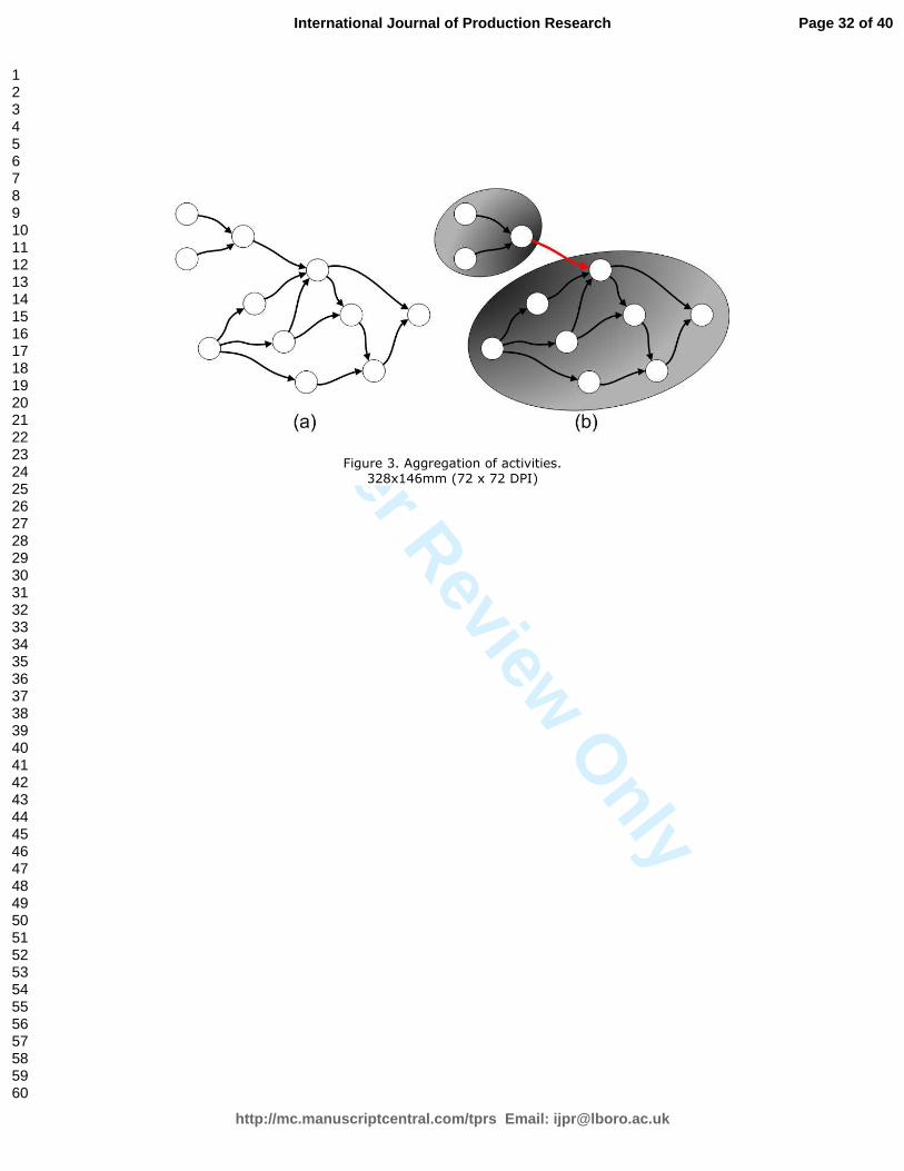
For Peer Review O

nly

Figure 3. Aggregation of activities. 328x146mm (72 x 72 DPI)

Page 32 of 40



123456789101112131415161718192021222324252627282930313233343536373839404142434445464748495051525354555657585960

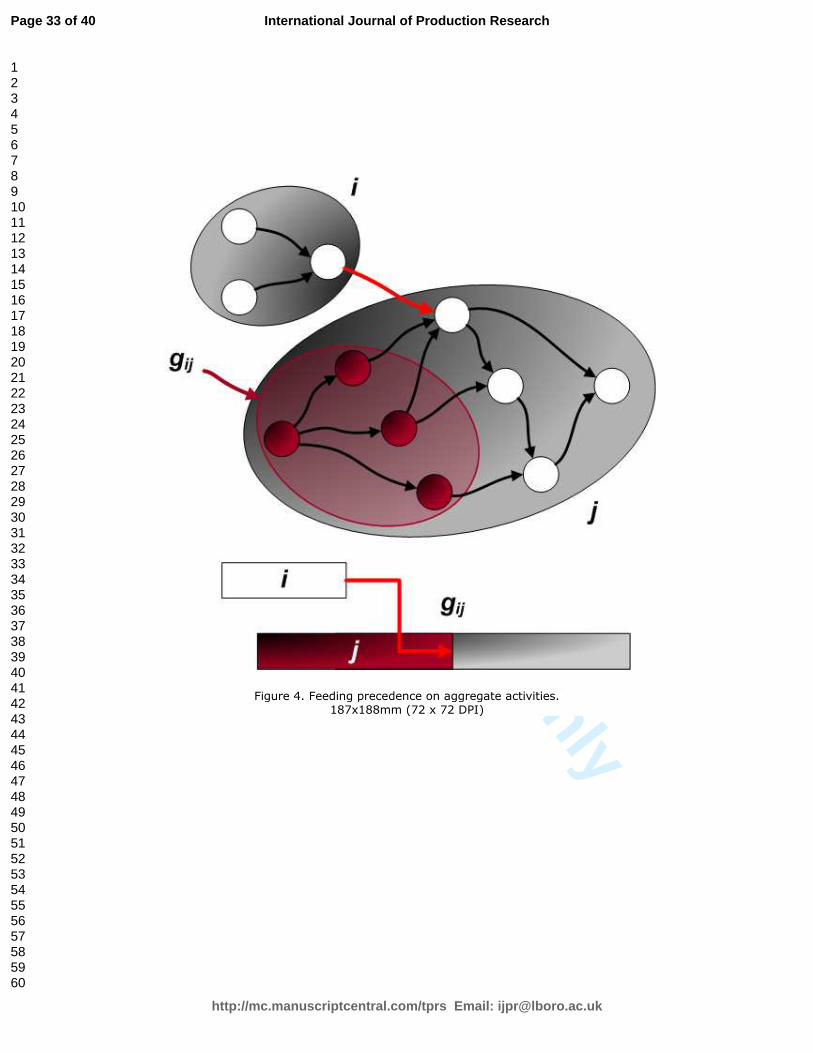
For Peer Review O

nly

Figure 4. Feeding precedence on aggregate activities. 187x188mm (72 x 72 DPI)

Page 33 of 40



123456789101112131415161718192021222324252627282930313233343536373839404142434445464748495051525354555657585960

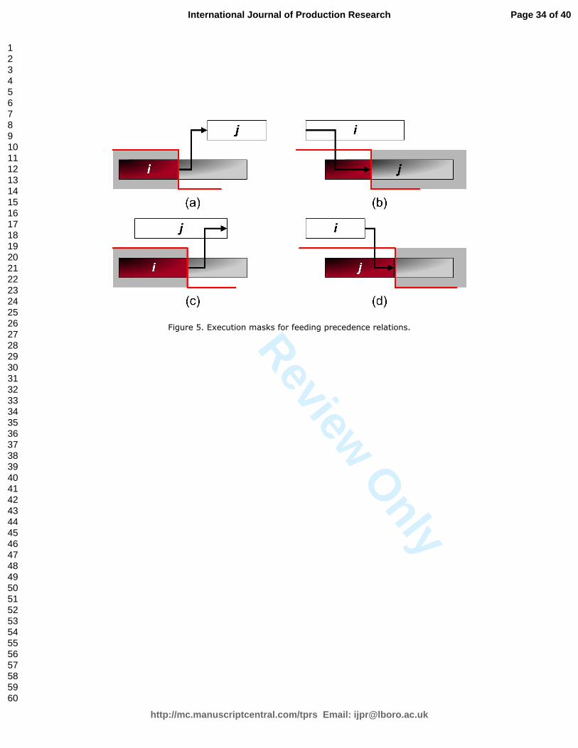
For Peer Review O

nly

Figure 5. Execution masks for feeding precedence relations.

Page 34 of 40



123456789101112131415161718192021222324252627282930313233343536373839404142434445464748495051525354555657585960

For Peer Review O

nly

Figure 6. Multiple precedence constraints.

Page 35 of 40



123456789101112131415161718192021222324252627282930313233343536373839404142434445464748495051525354555657585960

For Peer Review O

nly

Figure 7. Main Effects Plot for mean failures percentage.

Page 36 of 40



123456789101112131415161718192021222324252627282930313233343536373839404142434445464748495051525354555657585960

For Peer Review O

nly

Figure 8. Interaction Plot for mean failures percentage.

Page 37 of 40



123456789101112131415161718192021222324252627282930313233343536373839404142434445464748495051525354555657585960

For Peer Review O

nly

Figure 9. Main Effects Plot for mean solution time.

Page 38 of 40



123456789101112131415161718192021222324252627282930313233343536373839404142434445464748495051525354555657585960

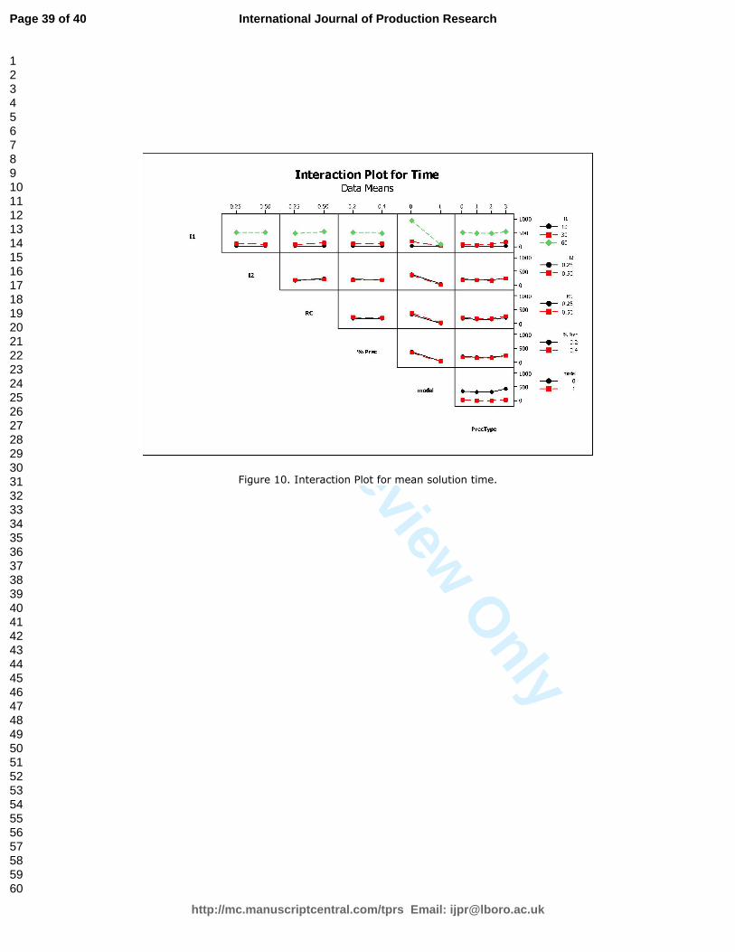
For Peer Review O

nly

Figure 10. Interaction Plot for mean solution time.

Page 39 of 40



123456789101112131415161718192021222324252627282930313233343536373839404142434445464748495051525354555657585960

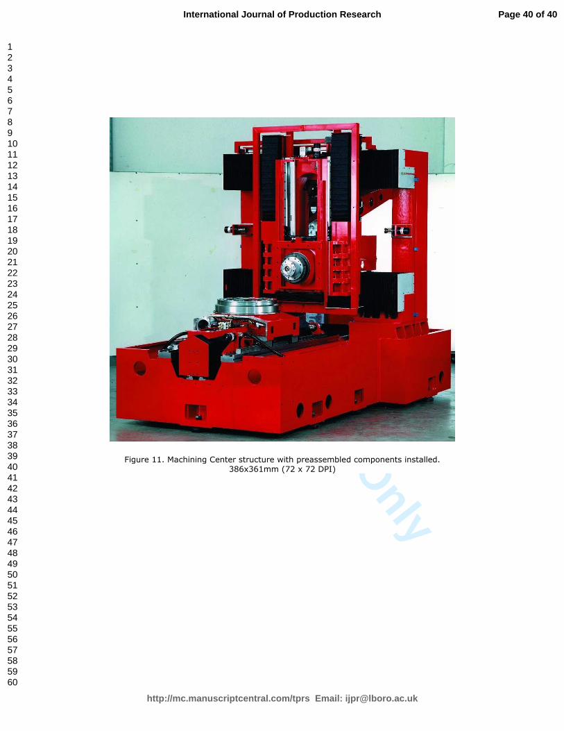
For Peer Review O

nly

Figure 11. Machining Center structure with preassembled components installed. 386x361mm (72 x 72 DPI)

Page 40 of 40



123456789101112131415161718192021222324252627282930313233343536373839404142434445464748495051525354555657585960

A Project Scheduling Approach To Production Planning with ...

Documents

Transcript of A Project Scheduling Approach To Production Planning with ...