Br. J. mtJU&. atatiat. Paychol. (1977), 30, 1-42 Printed in ~ Britain

A progressive approach to non-additivity and genotype-environmentaI covariance in the analysis of human differences.

L J. Eaves, KrystyDa Last, N. G. Martin and J. L J"mks

No aspect of human behaviour genetics has caused more confusion and generated more obscurantism than the analysis and interpretation of the various types of non-additivity and non­independence of gene and environmental action and interaotion-genotype-enviromnent interaction and oovariation, dominance and assortative mating. A comprehensive framework of theory and method is outlined in which these and other contn.outions to individual dif£erences can be critically assessed.

1. Introduction

There is a. view, widely held and frequently expressed, that genotype-environmental interaction (0 x lD) and genotype-environmental covariation (Cov OlD) are factors which preclude a worthwhile analysis of individual differences in human populations. Such is the view expressed in a variety of ways, for example, by Moran (1973), Layzer (1974), Lewontin (1974), Feldman & Lewontin (1975), and others. Whilst these authors allude to the possible importance of G x E and Cov OlD they offer no adequate specification of these effects, nor do they suggest how such effects may be detected.

There is, however, a large body of data and theory relating to the analysis of 0 x lD in species other than man (e.g. Haldane, 1946; Mather & Jones, 1958; Bucio-AIanis et al. 1969; Jinks & Perkins, 1970; Jinks & Connolly, 1975; Mather & Ca.liga.ri, 1975), there have long been attempts-not always successful-to specify CovOlD in man (e.g. Cattell, 1960; Loehlin, 1965), and a much-publicized paper by Jinks & FuIker (1970) deals with the principles and pitfalls in the analysis of both 0 x lD and CovOlD in man. In spite of a substantial1iterature in this area, there is still considerable ignorance about the theoretica.1 specification of these effects, their practica.1 analysis and their biologica.1 significance. In this paper we seek to clarify many areas· of misunderstanding surrounding all three aspects of the analysis of human differences .

.2. 'Assumptions' and scaling tests

The obvious needs to be stated. There are two types of assumption: those which can be tested, given adequate data, and those which cannot.. .An assumptiQn in biometrica.1 genetics is meant to be tested. The analytica.1 power of biometrica.1 genetics is due to the fact that assumptions are made not merely for the convenience of estimating parameters but in order that the model they imply might be tested. This fact is not always appreciated by critics who regard an assumption as a mark of weakness rather than as a. necessity for any attempt to test null hypotheses. A·study of individual differences which tests no assumptions about the causes of variation is little more than an exercise in the juggling of numbers. By contrast, the statistica.1 tests employed in biometrica.1 genetics, the so-called 'sca.Iing tests' (see Mather & Jinks, 1971, for a recent account), however simple or elaborate they may be, are developed precisely to test one or more assumptions a.bout the origin of differences. Much of our paper is

1

2 L. J. Ea1Je8, Krystyna Last, N. G. Martin and J. L. Jinka

devoted to a detailed examination of the methods by which particular assumptions may be tested and our confidence that such assumptions are adequately tested in practice.

3. Non-additivity

3.1. Ola88ijication

In our attempts to a.na.lyse variation we have to consider two types of non-additive effect which may contribute to individual differences, namely, genetical non-additivity and genotype-environmental interaction.

(a) Genetical 'TI.O'n-adti,iti1Jity •. Continued directional selection, acting on a trait, is expected to increase the relative importance of non-additive genetical effects, particularly directional dominance and epistasis of the duplicate-gene type (e.g. Mather, 1943, 1961, 1973; Breese & Mather, 1960; Broadhurst & Jinks, 1974).

There exist two fundamental misconceptions relating to the analysis and biological significance of non-additive gene action. One is typified by Feldman & Lewontin (1974) who claim, on the basis of a purely mathematical argument with no experimental foundation, that selection. should eradicate additive variation almost entirely whilst leaving a great surfeit of dominance for traits related to fitness. They have misunderstood the basis of the argument which rests not on algebra but experiment. The trait is unknown to quantitative genetics for which non-additive variation exists without a substantial additive component. Numerous experimental studies suggest that genetical non-additivity is expressed against a background of additive gene action for traits related to fitness.

The second misunderstanding is illustrated by Morton (1974) who asserts: 'The notion of dominance deviations. for polygenes seems far fetched'. That this is untrue will be attested by any practical quantitative geneticist with experience of the importance of dominance and epistasis in organisms other than man (e.g. Comstock & Robinson, 1952; Jinks, 1955j.Breese & Mather, 1957, 1960j Jinks & Jones, 1958; Kempthorne, 1960; Jinks & Broadhurst, 1963; Hanson & Robinson, 1963; Jinks & Perkins, 1969, 1970a).

At the very simplest level the superior vigour of commercial F 1 and double cross hybrids and the ubiquity of inbreeding depression in outbreeding species are common­place manifestations of non-additive gene action. Certainly Morton, advocating path coefficients as an analytical device. is faced· with a conceptual difficulty in the analysis of any kin~' of non-additive variation but it is mistaken to ignore such aspects of proven

. significance in other organisms merely because their analysis in man is more difficult. Indeed, as Morton and his associates refine their approach in an attempt to include non-additive effects the method should become very similar to that of biometrical genetics and ought to give the same answer with adequate data.

(b) Ge:notype-en1Jironmental interaction. Whilst some authoritative writers have attempted to justify the assumption of genetical additivity. perhaps in order to simplify the processes of specifying models and estimating their pa.r8.meters. several others have lent their support to another view that G x E is by contrast a widespread and substantial component of individual differences. At the same time, it is suggested, G x E effects in man are both substantial on the one hand and undetected on the other, with the implication that attempts to estimate and interpret other population parameters are thereby seriously in error.

Animal and plant experiments certainly demonstrate that G x E is widespread whenever a set of genotypes is grown in a variety of controlled or even uncontrolled

environments. In recent years, there has been considerable success in the detection, analysis and interpretation of G xE. It is dangerous, however, to exaggerate the general significance of G x E. If variation in man has any similarity to variation in other organisms we would conclude that a trait was atypical. if more than about 20 per cent of the measured variation could be attributed to G x E, An effect of this :tna.gnitude would be' important but not overwhelming. We shall consider the feasibility of· detecting such. effects in man.

3.2. 8yatemaJ.ic aM. 1W'n-syatematic effects

Before we can attempt to analyse non-additive effects,much less presume to comment on their significance, we must recognize the practical distinction between:

(a) systematic ('directional" or 'sca.1a.r') effects·; and (b) unsystematic ('ambidirectional') effects. .

This distinction is important in the consideration of genetica.l non-additivity and genotype-environmental· interaction for both practical and theoretical reasons.'

At the level of practical analysis both kinds of effect contribute to variation and so we can expect that they will contribute to second-degree statistics, i.e. to variances and covariances of raw observations. Thus, for example, all genes showing dominance will tend to increase variability and so contribute to the non-additive component of second-degree statistics. On the other hand, first- and third-degree statistics will only be affected by non-additive effects if there is a net directional component. Thus, only directional dominance (as opposed to ambidirectional dominance) will result in inbreeding depression or in skewness within segregating families. A similar distinction is essential with respect to G x E. Although all kinds of G x E contribute to second-degree statistics, detailed analysis of G x E in experimental orga.njsms suggests that part, often a. substantial part, of the G x E variation is due to the effects of genes which are associated in effect or distribution with the genes which contribute to the differences between genotypes averaged over environments (e.g. Perkins & Jinks, 1968, 1973; Fripp & Caten, 1973; Mather & Ca.ligari, 1975). Such associations can often be broken by artificial selection (Perkins & Jinks, 1968, 1973; Brumpton, 1973; Jinks & Connolly. 1975), which implies that they may well have been maintained solely by natural selection. The very fact that G x E exists at all means that sensitivity or reaction to the environment is itself under genetical control, and may consequently be altered by selection just as selection may change or stabilize any other aspect of the phenotype which. is under genetical control.

Both directional non-additive genetical effects, among which we include directional dominance, and systematic G x E interaction of the type we have discussed. may contribute to third-degree statistics. Jinks & Fulker adapted the methods used for the detection of such G x E to the detection of systematic G x Ein man. We shall see that only a relatively small part of the environmental variation need be due to genes associated systematica.lly with overa.ll genetical differences in order to be detecped by their approach. The practical importance of such systematic interactions is that they allow a measure of prediction about the relative efficiency of the same degree of environmental manipulation at different points of the scale of measurement.

3.3. N Q1&-additi1Jity and 8Cale

In a recent book, Kamin (1974, p. 152) dismissed an a.na.lysis. of genotype-environment interaction for a cognitive trait on the grounds that: 'Whether or not we observe an

4: L. J. Ea'IJe8, Kry8tyna £aBe, N. G. Marlin and J. L. Jin/ca

interaction depends upon our choice of scale. The choice of scale is arbitrary-as is the advice provided to educators . . . .' In fact, of course, quantitative predictions of any kind are dependent on the choice of scale. This fact is rarely understood outside those areas of biology and psychology in which the attempt to make quantitative predictions flourishes, albeit prematurely in some instances.

Virtua.1ly a.ll kinds of systematic nOll-additive effects could be removed by a change of scale, either by a simple tra.nsforma.tion or by altering, in a psychometric study, the difficulty and discriminating power of the items which constitute a particular test. By altering the re1a.tive amounts of information at different points in the scale of individual differences the psychometrician is altering the re1a.tive weightings given to different gene substitutions and environmental circumstances. He is thus, whether he likes it or not, adjusting the epistatic and genotype-environmental interactions expressed in the trait he is measuring. A change of scale is a change of trait. We sha.1l see that the same items, handled in slightly different ways, give ra.dica.lly different pictures for the causes of individual differences. As long, however, as a particular scale is used for measurement and prediction, we are forced to accept whatever complications may be required in order to exp1a.in the causes of variation on that scale. It is a fa.1la.cy to suppose that there is a 'true' scale. Any scale is arbitrary. There are merely scales which are more satisfactory for some purposes than others. It is a.lso a fal1a.cy to suppose that a scalar transformation to remove non-additivity is rea.lly only 'hiding' the interaction.. Gene substitutions and environmental effects have to be measured by their effect on the phenotype at some level or other. Often there will be conflict about the choice of scale because it is not to be expected that genetical and psychological considerations will always coincide in suggesting a choice of scale. A scale which satisfies a criterion of genetical additivity may be subject to geno~nvironmenta.1 interactions and vice versa. A trait which has desirable genetical properties may display a complex and undesirable re1a.tionship with some external criterion va.ria.ble.

The existence of genetical and genotype-environmental interactions of a. systematic variety may alert the psychometrician to areas in which farther test development may take place. Marked directional non-a.dditivity, for example, may indicate a threshold in the scale beyond which measurement is difficult, or ha.s simply not been attempted. We shall consider the consequences of different forms of scaling later.

The so-ca.lled 'problem of scale' is only a problem for those whose scientific inquiry has never proceeded beyond the limitations of broad qua.1itative statements unsupported by measurements. The long-standing use of the term 'sca.1ing test' to the variety of methods used in biometrical genetics for the detection of many kinds of non-additivity is a. testimony to their dependence on the scale used. The criteria of sca.1ing are many, and will depend on the principal theme of a. particular inquiry. Few, if any scales will satisfy a.ll criteria. A particu1a.r choice of scale will be vindicated by the successful predictions it facilitates. In a biometrical-genetical context the situation is summarized simply by Mather & Jinks (1971, p. 63) in the following way:

The scales of the instruments which we employ in measuring our plants and animals are those which experience has shown to be convenient to us. We have no reason to suppose that they are specially appropriate to the representation of the characters of a living organism for the purposes of genetical analysis. Nor have we any reason to believe that a single scale can reflect equally the idiosyncrasies of all the genes·affecting a single character ••.• The scale on which the measurements are expressed for the purposes of genetical analysis must therefore be reached by empirical means. Obviously it should be one which facilitates both the analysis of the data and the interpretation and use of the resulting statistics.

Lord & Novick (1968, p. 22) state a similar view in a psychometric context as follows: 'If a particular interval scale is shown empirically to provide the basis of a.n. accurately predictive a.n.d usefully descriptive model, then it is a good scale and further theoretical developments might profitably be based on it. Thus measurement (or scaling) is a fundamental part of the process of theory construction.'

4. Non-independence

The second major class of assumptions which a.re cha.ra.cteristic of preHminary attempts to explain human differences relate to the independence of genetical and environmental effects. Gene effects may be correlated inter 8e as a result, for example, of linkage disequilibrium stemming from assortative mating. Genetical a.n.d environmental effects may be correlated for a variety of reasons, including cultural transmission a.n.d sibling effects.

4.1. A.88orlative mating

The literature on assortative mating has recently been revived because of several papers dealing with aspects of Fisher's (1918) treatment of assorta.tive mating, for a long time the basis of most analyses of the human mating system. As with all theoretical debates it is difficult to decide always whether various criticisms point to elTOrs of argument which lead to serious errors of interference, or whether they a.re merely differences in degree of approximation well beyond the resolution of most practical studies. In the fina.l analysis,a.n.y theoretical considerations must sta.n.d the test of data. Wilson (1973), for example, has argued that assortative mating without selection is unrealistic a.n.d offers a generaJ.iza.tion of Fisher's approa~h which can take account of the fact that extremes may find it more difficult to mate. The practical crux of her theoretical argument rests on whether or not the population of spouses is significantly unrepresentative of the population of genotypes from which they a.re drawn. In a large and detailed study such differences a.re almost certain to be detected. Vetta. & Smith (1974), however, have cast some doubt upon the correctness of the mathematical argument advanced by Wilson. Until this issue is resolved any practical application of her model must wait. On the other hand, Vetta & Smith (1974) and Vetta. (1976) have examined Fisher's argument in great detail a.n.d have generally satisfied themselves of its mathematical propriety, even if they and others have some reservations about its likely practical application. In a recent communication, Vetta. (1976) has suggested that Fisher's expectation for the parent offspring correlation is slightly in error because assortative mating is expected to introduce some covariation between the dominance deviations of parents and offspring. He examines the data analysed in Fisher's original paper and confirms that Fisher's estimates of genetical parameters are in error in the second a.n.d third significant figures (personal communication). Such differences, whilst no doubt mathematically significant, do not come within the resolution of practical studies at the present time. In fact, wherever Fisher's model of assortative mating has been applied and tested-{see e.g. Eaves, 1973, 1975), the fit to real data has been fairly good. This is not to claim that other models of assortative mating might not give as good, or even better, fit. But we should bear in mind that in the last _analysis more extensive data,and not mathematical theory, are the only way of resolving the practical issues.

The problem of assortative mating illustrates a more general problem in quantitative genetics, particularly when its methods a.re applied to man, and that is the problem of

6 L. J. Eaves, Krystyna Last, N. G. Martin and J. L. Jinks

resolution. Although we may list the many factors which contribute to human variation, we are only likely to detect some factors if they account for a considerable, and sometimes a very considerable, proportion of the variation. We shaJI discover this as we consider our ability to detect various effects later in this paper. The extent to which we can detect a given effect will always depend on its nature, its magnitude and the experimental design. Some effects can be detected with great certainty, others with great unreliability. In our experience of the analysis of human data, it is possible to show that some effects which account for as much as 20 per cent of the total variance are beyond resolution in. unfavourable circumstances.

At the present time, therefore, our aims have to be much more modest than those of· correcting the second and third signiiicant figures of our·estima.tes of parameters. We have to concentrate 'on testing those assumptions which we know to be testable in principle and whose failure could lead to major errors of inference.

Thus, with reference to assortative mating, it is a trivia.! task to demonstrate a marital correlation for a. trait. It is slightly more exacting to demonstrate that such a correlation is having the expected genetical consequences in human populations. Eaves (1973) showed how the genetical consequences of assortative mating could be detected iD. one population.without reference:to the marital correlation. Many studies of.IQhave suggested that the linkage disequilibrium resulting from assortative mating is having, a' . significant·effect on the amount and.distribution of genetical variation in human populations. Even a.t· this level, however, we ha.ve to recognize that studies with. dimensions of those usually performed will·almost. certainly be unable to. detect the genetical' consequences of assortative mating unless there' is considerable additive genetical variation for the trait under considera.tion~ Furthermore, although under such circumsta.nces·.we may be 'satisfied that a; theory such as Fisher's is adequate to explain the variation, we would be more dubious about excluding a. variety of deriva.tive theories whioh predict very simila.r. consequences. .

One aspect of assortative mating theory which could.quite easP.y become the basis· of empirical study is the precise rela.tionship between the various kinds of correlation between spouses. Most pra.ctical trea.tments have assumed that .the genotypic correlation between spouses is a. pale reflection of the phenotypic correlation between spouses, and tha.t the latter is properly estimated from the correlation of measurements made on' a single occasion. When Eaves (1973)' attempted to estimate the degree of assortative mating for IQ without reference to the marital· correlation and then employed the genotypic correlation to predict the correlation 'between spouses, it was found that the predicted marital correlation was closer to, the observed value after correction for unreliability than to the raw correlation between pa.rental IQ scores. Although it would be a mistake to use.suohnon-significant differences as any more than a starting point for discussion, it does illustrate the possibility tha.t the human organism, integrating data over a wide range of oocasions and encounters, may achieve a more aocurate assessment (albeit unconscious) of .the innate abilities of potential mates than is provided by explicit psyohological tests.

Fisher himself expressed doubt about the exact relationship between the phenotypic and' genotypic correlations between spouses and gave different sets of expectations for the correlations between relatives depending on the precise model which was assumed for assortative mating. Generally it has been assumed (and not disproved) that the genetical correlation between spouses is a seconda.ry consequence of their phenotypic correlation.

Fisher's treatment of assortative mating, and indeed many of the alternative approaches, assumes that genetical and environmental factors are additive and

independent. It is not easy to see how damaging genotype-environment interaction would be for the specification of assortative mating using Fisher's approach. In so far as the genes affecting sensitivity to the environment· are independent in effect and distribution with respect to those which determme overall differences for the trait on which. assortative mating is based it is difficult to see how the approach can be seriously in error. We can see, however, that, perhaps as a result of assortative mating or selection, the genes responsible for stability may become associated systematically with those which detemrine a particular overall expression of the trait in question. Thus, for· example, it is not beyond the bounds of possibility that a, genetical system could have evolved in which the genes which increase intelligence are associated with genes which promote stability of gene expression in a wide range of environments. Systematic G x JiJ interactions· of this type, however, are precisely those which the approaches of biometrical genetics, exemplified in this context· by the approach of Jinks & FuIker, are most able to detect. In practice, Fisher's model of assortative mating has not·been used, and we doubt whether it should be used, when systematic G x JiJ interactions are known to be present.

The independence of genetical and environmental factors is the basis of Fisher's treatment of assortative mating. There seems still to be some confusion about the precise content of the.assumptions that Fisher made in deriving his expectations. Providfug environmental factors remain independent of genetical differences it·does not matter for Fisher'smode1 whether or not the environmental deviations are correlated for individuals reared in the same family. Once the quality of the environment in which a family develops depends on the genotypes of the parents who provide the environment (i.e. in, the presence of cultural transmission), then individuals' genotypic deviationS are no longer distributed independently of their environmental differences and Fisher's model may not be applicable to individual differences in the presence of such genotype-environmental covariance.

4.2. Gen.otype-envir01l1llunt COtJariance

Cattell (1960) was one of the first authors to consider Seriously the consequences of the possible covariation of genetical and environmental effects in human populations. The weakness of his approach, and virtually every subsequent approach to the problem, has been the lack ·of any precise theory fo~ the origin of genotype-environlnent covaria.tion (Cov GE), which can be cast in a quantitative form to allow any parsimonious and powerful treatment of variation in the presence of CovGJiJ. The specification of Cov GJiJ is plagued by empiricism. As recently as. 1975, Thomas maintained in connection with CovGJiJ: ' ... precisely how these terms may be viewed may be in dispute because substantive theory is lacking'. The fact that so· many attempts to specify CovGJiJ have come to grief is because their authors have thought in statistical rather than biological terms. Their approach has been to write in a model virtually every conceivable covariance term involving genetical and environmental effects, and then to decide, by intuitive arguments, which genotype-environment correlations could be set to zero and which could be regarded as equal for the purposes of estimation. Often, as is the case most recently in Thomas' (1975) approach, there is no a.ttempt at all to decide what restraints may operate upon the parameter values, with the result that quite arbitrary and misleading restraints are applied merely to obtain a solution. Indeed, Jinks & Eaves (1974) used the approach of specifying arbitrary restraints in order to solve for genotype-environmental correlation in an a.nalysis of

8 L. J. Eaves, Krystyna Laat, N. G. Martin and J. L. Jinka

IQ da.ta. This approach is undesirable, and is a poor substitute for a theory which enables us to see quite clearly the relationships between genotype-environment covariance parameters in different kinds of statistics.

The classical approach is to specify CovGE in terms of a genotype-environmental correlation (r gJ and the genotypic and environmental standard deviations (era and ere). This is the approach of Cattell (1960), Loehlin (1965), Jenks et ale (1973), Hogarth (1974), Jinks & Eaves (1974), Jensen (1975), Thomas (1975) and Goldberger & Lewontin (1976).

This approach is deficient. The relative magnitudes of r 118 in different kinds of family are determined by the source of environmental variation which covaries with genetical differences. For example, when the genotype-environmental correlation arises because one sibling forms a developmentally significant part of the environment of another, the environmental variation and the genotype-environmental covariation resulting from this can be specified precisely and economically in a way that leads to testable hypotheses. However, the 11S1l&l approach, through the specification of r 118' leads to an unnecessary multiplication of parameters because the genotype environment . correlation and the environmental variance are interdependent in a way which depends on the degree of relationship.

In fact, it is possible, as Eaves (1976a, b) has shown, to parameterize genotype­environment covariance in a variety of ways consistent with meaningful biological and psychological theories. We may distinguish the following three kinds of CovGE which can be specified in terms of a theoretical model. Two of these can be detected by quite simple studies.

(a) Environ/me-rUB selected by genotypes. In the event of superior genotypes seeking or establishing for themselves advantageous environments, that part of the environmental variation and the CovGE which depends on genetical differences between individuals will be confounded with estimates of genetical variation. Any analysis of individual differences in a single culture, at a single point in time, will be unable to separate the 'direct' effects of the genes from those which operate through promoting selection of, or change in, the environment. Further, gene expression may be altered as a result of cultural change. A freer, more mobile society might display greater genetic variability because individuals are free to select the environment in which they develop. A restrictive more static society may reduce genetic variability in a variety of ways, simply by preventing genotypes from selecting or creating their own environments. Such changes in genetical variability resulting from the stimulation or suppression of one source of genotype-environment correlation may also be regarded, in another light, as a form of genotype-environment interaction. Because, in general, we are only able to assess the performance of any given array of genotypes within a single culture it may be difficult to design clear-cut demonstrations of this phenomenon.

(b) Sibling effects. Human beings often develop in the presence of siblings. Identical twins develop in the presence of a sibling of identical genotype; foster children may be raised in the presence of a sibling who is genetically unrelated. If the behaviour of siblings is important in development, either because siblings compete for a.vailable resources or cooperate in obtaining resources, then a cha.ra.cteristic pattern of CovGE may emerge which can be clearly identified (Eaves, 1976a). Under these circumstances the genotype-environmental correlations are expected to show a complex functional relationship which is better represented by a simple model that recognizes those linear relationships expected to exist between the genotype-environmental covaMnces.

(c) Oultural transmia8ion. Perhaps the most significant area. of concern, at least theoretica.lly, is the extent to which cultural transmission is an important component of individual differences. Cava.11i-Sforza & Feldman (1973) have renewed interest in this area by offering an approach in which the effect of the phenotype of one individual (in this case a parent) influences environmenta.lly the phenotype of another (in this case an offspring). Eaves (1976b) has examined severa.! of the consequences of this approach for the analysis of randomly mating populations, and shows how cova.ria.nce of genetica.1 and environmental differences between fa.m.ilies may be a consequence of cultural transmission perpetuating differences whose origin is ultimately genetica.1. As with the case of sibling effects, the effects of cultural transmission can be specified parsimoniously in terms of a mathematica.1 model which suggests that cultural transmission has its own pattern of Cov G1i1 for which diagnostic tests are simply devised.

The importance of genotype-environment covariance- is twofold. Genotype­environmental covariance of the kinds we have distinguished is only possible if genetica.1 influences are modifying the quality of the environment. The detection of Cov GJil is thus important psychologica.1ly since it draws our attention to the personal aspects of an individual's environment rather than to the accidents of development. People become more significant in the environment than materia.! things. Secondly, the detection of Cov GJil may be important biologica.lly because a population in which one genotype can affect the performance of another is a necessary prerequisite for any system of evolution by group or kin selection. It may be that CovGJil could provide some basis for deciding between traits on which natural selection operates on an individual basis, and those which may be subject to kin selection.

One form of CovGJil we have not considered is that which arises because of pla.cement. There is inevitably an element of empiricism in the specification of such models, but perhaps even here theories about placement may be given some more concrete and testable form. Subsequently we sha.ll consider in more detail the specification and detection of the various forms of genotype-environmental cova.rla.nce. Although we consider only the specification of CovGJil for randomly mating populations and although an adequate theoretical specification for assortatively mating populations may still be elusive, we should note that the genera.! consequences of the different kinds of Cov G1i1 will persist whatever the mating system and for this reason we must not be misled into thinking that Cov GJil is not detectable in the presence of assortative mating. In this respect the scaling tests we propose for the presence of CovGJil are sca.1e free. In the presence of detectable CovGJil, however, especia.llywhen this is due to cultural effects (i.e. involving the covariance of genetica.1 and environmental differences between families such as Jinks & Fulker suggested might be the case for educational attainments), we suspect that any further attempts to analyse gene action when there is assortative mating should be resisted until an adequate theoretica.1 specification of the joint effects of mating system and culture has been realized.

5. Elementary considerations

When we are faced with the genetic analysis of any body of data several questions occur which form the basis of the subsequent a.na.lysis and interpretation:

(I) What are the appropriate statistics for summarizing the data. prior to a.na.lysis 1 (2) What set of assumptions is it proposed to test and how might they be formulated

in terms of a quantitative model 1 (3) What scaling tests can be devised to facilitate the testing of these assumptions

and how might the parameters best be estimated 1

10 L. J. Eaves, Krystyna Last, N. G. Marlin andJ. L. Jink8

(4) Given that a simple model fa.iIs how might it be extended 1 (5) How powerful are these tests given the structure and size of the sample 1 (6) How serious are the elTors of inference which may follow from failure to disprove

an assumption which is, in fact, false 1 It may be thought that these questions are too basic to need repetition, but it is

our view that more confusion stems from failure to consider these matters carefully than from any other. We now consider the:first three issues, and defer exa.mi.na.tion of the other three to later sections.

5.1. ChoiCe o/statiatic

For too long the colTelation coefficient has been adopted as the starting point for an analysis· of individual differences. Cattell's MA V A and the biometrica1 genetical approach are exceptions to what is virtually universal practice. Whatever the. appeal of the intraclass cOlTelation as a number, and however much we may be forced into using it: beca.use it is the statistic used in the past, we must recognize that simple­minded use of the cOlTelation coefficient may well lead to the obscuring of highly . significant features of the genetical and environmental system, to inefficient tests of others and to· undetected. biases in estimates of .parameters. COlTelations· are· only an effective starting point for an analysis of individual differences when the causes of individual differences are fairly simple. Otherwise information is wasted in the . standardization· of the different groups of data .. to unit variance. This is partic1ila.rly misleading if hypotheses are to be tested· whose failure is most clearly to be seen in. a pattern of total. variances. Thus, for example, one of the :first signs of sex-linkage or sex-limitation may- be a difference between the total variances· of the two sexes. .. More important, however, is the expected pattern of total variances for different.groups of individuals in the presence .. ofgeno~nvironmenta1 covariation. Such differences are better analysed than removed by a purely statistical device.

We can illustrate the problem by reference to a simple example. Consider the. analysis of monozygotic twin data in the presence of covariation of genetical and environmental differences between families. Suppose we·have data on twins reared together and twins reared apart in randomly chosen foster· homes. Differences within· pairs of twins reared apart will be due to within- and between-family environmental influences (EI and Es respectively). The component of variance between such pairs will refiect only genetical differences (G). For twins reared apart,. there is expected to be no Cov GE. For twins reared together, variation within pairs will re:B.ect simply environmental differences within families (E1) whilst differences between pairs will re:B.ect G, Ei and, in the presence of geno~nvironmental covariance,.1lI contribution from this source. (CovUses)'

If we start with the raw data,· and derive the mean squares of the analyses of variance within and between pairs for each twin type (i.e. producing four mean squares in all), we have four statistics and four parameters (G, E I , Ea and CovUses), as shown in Table 1. Thus, a perfect fit solution can be obtained to give estimates· of all the parameters and to yield tests of significance of the parameters, although no further test of the model is possible and no further investigation of the genetical system can be undertaken. If we now standardize the data to give- intrac1ass COlTelations, we have only two statistics, namely, the colTelation of MZ twins reared apart and that for twins reared together. Although we can introduce one arbitrary constraint on the parameter values (e.g. that G+El +Ea is unity), we still have three free parameters in our model with only two statistics available for their estimation. This means that, by

N on-additi'lJity and ge:notype-ell/viron'lTUinial covariance 11

taking intraclass correlations, we have made it quite impossible to estimate the rela.tive contributions of genetical and environmental effects and their cova.ria.tion. By taking correlations information bas been lost, in this instance to the point of making any solution impossible. This is an extreme example, but the general principle remains that standa.rdiza.tion to unit variance reduces the power of certain crucial tests of assumptions which are comparatively powerful when the analysis of var.ia.nce is used as a starting point for the analysis.

Table 1. Expectations of variance components for monozygotic twins reared together and apart (MZT and MZA), in the presence of covariance between genotypic and environmental differences between families

G El E, COVgI 8.

BetweenMZT 1 1 2 WithinMZT 1 Between MZA' '1 Within MZA 1 1

We have laboured this point because Morton (1974) has, for statistical rather than biological reasons, expressed the opinion that: 'The estimation theory should be, developed in terms of the z transform ofcorre1a.tion, for which the normality assumption is less restrictive. Clearly, emphasis must be on tests of hypotheses rather than on estimation.' In fact, the approach. to estimation advocated by Morton is that rejected by eXperienced quantitative geneticists preciSely because it·ignores many of the simple and powerful tests of hypotheses available with the raw statistics. At best there will . be a loss of information; at' worst parameters will, not be estimable and' any estima.tes which are obtained may be seriously biased (see Jinks & Fulker, 1970, pp. 324:ff.). Whatever'the practical and statistical convenience of the correlation coefficient, it is not an appropriate ,starting, point for model fitting. .

Instead, following the long experience of biometrica.l genetics, we start with the data summarized in terms of analyses of va.ria.nce, identifying, for example, the mean squares within and between families; or, in, cases, where the analysis of variance might be inappropriate, we start with variances and covariances between relatives, for example, the variances·and covariances of parents and offspring.

5.2. Fqrm,uliuing a motkl for individual ai!ferf?/Me8

Anyone can write a model but there is little point in doing so' unless the model embodies a testable null hypothesis. Often a simple model might be written which could fail in practice fora variety of reasons. Sometimes a model may fail but we may be unable to decide exactly what is causing the failure with the data available. Thus, for example, we may represent in a model the null hypothesis that the data give no reason to doubt the randomness of mating, the additivity of gene action, the absence of cultural effects and genotype.-environment covariance, and the equality of environmental variances for different kinds of relatives. Such a simple model can be written and tested, even with data on identical and fraternal twins reared together. Any of the factors excluded in the null hypothesis might cause failure of the model, and although we might be able to find further data which suggest what is contributing to the inadequacy of the simple model, the twin data by themselves will be inadequate for this purpose. Thus, for

12 L. J. Eaves, Krg8tyna Laat, N. G. Martin anti, J. L. Jinks

example, it is sometimes taken as self-evident that the environmental differences within MZ twins are sma.ller than those of DZ twins. H this is the case, then a simple model which assumes comparability of environments should fail. Otherwise we have to conclude that we have no evidence to support the view that environments of twins depend on zygosity.

Clearly, it would be impossible to give a full account of the specification of every possible set'of circumstances for a.ll kinds of relationships. Many of the possibilities are already in the literature (e.g. Fisher, 1918; Eaves, 1969, 1973, 1976a, b; Jinks & Fulker, 1970; Eaves & Eysenck, 1975, 1976). Here we intend to give expectations which illustrate certain basic principles of model building. for a particular set of relationships.

(a) A hypothetical experiment. We shaJl illustrate the principles of model building and testing by reference to an experimental design which is rather more demanding than those usua.lly employed in psychogenetical studies in order that we may see how different effects are likely to be detected more easily in some sets of data. than others. We choose the design to cover the widest range of possibilities for the causes of individual differences, whilst still restricting ourselves for convenience to those situations where the model is linear, or can easily be linearized.

We will consider the different theoretical expectations which could be applied to statistics derived from the following kinds of data.:

Monozygotic twins reared together; Dizygotic twins (full-sibs) reared together; Monozygotic twins reared apart; Dizygotic twins (full-siblings) reared apart; Unrelated individuals reared together; and Singletons, reared by their natural parents.

In practice, in order to specify correctly any model for sibling effects it is necessary to know more about the rearing conditions of those related individuals who have been reared apart. We sha.ll give the expectations for such individuals on the assumption that they have been reared as singletons in randomly chosen foster homes. Other expectations would apply if individuals were reared with other natural or foster siblings, or reared, for example, by relatives. Similarly, our expectations on the basis of cultural transmission assume random placement. Genera.lly speaking, placement seems to be a significant factor in many studies of IQ.

The effects of placement on the similarity between members of a family will depend on the principles on which their placement is based and on the major causes of individual differences. In most cases placement effects should produce results which are inconsistent with any simple model which assumes their absence. At one extreme, for example, if individual differences are largely inherited, placement can have little effect on the similarity of relatives reared apart, but will be reflected in a large (genetic) correlation between unrelated individuals reared together. On the other hand, if cultural effects predominate in the determination of individual differences, the differences between families of unrelated individuals reared together provide an upper limit to the effects of cultural differences and are expected to be not substantia.lly affected by placement. When cultural effects predominate, related individuals reared apart are not expected to be more alike than unrelated individuals reared together however marked the effects of placement.

(b) The baaic model. The simple model on which we build is that adopted by Jinks & Fulker (1970) in their discussion of the relationship between biometrical genetical approaches

and those proposed by cattell in the multiple abstract variance ana.1ysis (MA VA). Though in many respects this model is not suitable in genera.! because of its reliance on purely empirical pa.ra.meters, it provides a valuable starting point for discussion, providing that we restrict ourselves to consideration of the groups of relatives we have already enumerated above. Given that a.ll the groups of relatives represent random samples of the population of genetical and environmental in1iuences, then in the absence of genotype-environmental interaction and genotype-environment correlation, we expect the total va.r.ia.nces of the groups to be equa.!. We may then write for each group the same expectation for the total va.r.ia.nce:

(Tps = O+E.

This formulation is not very helpful, however, because it does not recognize the different ola.sses of genetical and environmental variation which contn"bute to 0 and E. We may a.na.lyse 0 in two ways. The first approach, which is that of MA V A, is to recognize that individuals differ genetica.lly because their particular parents bear a restricted selection of the ava.ila.ble a.lleles in the population. That is, families differ genetically because their parents differ. Such differences contribute to the between-family hereditary variance, O2 in the notation of Jinks & Fulker. Within families, however, individuals differ as a result of segregation of the a.lleles from the parental set. Segregation contributes to the genetical variance within families. This contribution we denote by 01 0 This is one approach, which is satisfactory providing we consider only the groups or-relatives here. Once we consider other kinds of relationships. parents and offspring, for example, or cousins, this approach leads to a dead end because new parameters have to be introduced to specify each new situation. Differences can always be explained in this way, but no true analysis is possible. This is the weakness of the M.A YA approach. By contrast the biometrical genetical approach parameterizes the genetical components within and between families in terms of a few general parameters which specify the cumulative additive and non-additive effects of genes and which·can be used to describe the contribution of genetical factors to any kind of variance or covariance in a population. When mating is random, for example, the additive and dominance effects of autosomal loci can be represented by parameters DB and HB respectively, thus: .

0== !DB+ iHB'

O2 == iDB+.r,.HB,

01 == iDB+irHBO

Providing that the genetical assumptions are met, then other variances and covariances for randomly mating populations can be represented in terms of the same two pa.ra.meters. We have not specified the effects of epistasis. Although this can be done (see Mather, 1974), we have not done so here because so much of the variation due to epistasis will be correlated with the factors contributing to the dominance parameter, HB , that residua.! epistatic effects are likely to be too sma.ll to be detected against the background of other more significant effects; that is, although fitting only DB will leave some epistasis in the residuals, adding HB will account for virtua.1ly a.ll residua.! non-additivity. .

The effect of assortative mating is to generate linkage disequilibrium between the loci affecting a trait and to produce a slight increase in homozygosity. When many genes are involved, however, the effect of linkage disequilibrium on the genetic variance is

14 L; J. Eaves, Kry8tyna Last, N. G. Marti'll, arul J. L. Jinks

very much more marked than that due to increased homozygosity; indeed, the effect of the latter on individual differences is very slight; The linka.ge disequilibrium, however, leads to a substantial increase in genetical differences between fa.milies. Fisher (1918) showed that, if a population was in equilibrium under assortative mating, the genetical variation between families (02) was increased by an amount tDR(.A/(l-.A»~·where A represents the correlation between the additive geneticaJ. deviations. of spouses. The relationship between A and the marital oorrelation will depend upon, among other things. the narrow heritability of the trait and upon the precise basis on which assortative mating takes place. The general effect of assortative mating.is to. make distant relatives much. more alike than might be expected on the basis of a random mating model. This fact has been exploited to provide quite a powerful test of the genetical consequences of assortative mating (Eaves, 1973). . . .

Whereas we have a ready-made theory of genetical factors which can be cast into a precise and testable mathematical form, there is a general deficiency of rigoroUs modeJ.s for environmental variation. Although some steps have been made towards improving this situation, for example in the specification of maternal effects (Mather & Jinks, 1971), cultural effects (Cavalli-Sforza & Feldman, 1973; Eaves, 1976b) and sibling effects (Eaves, 1976a), we must be prepared to accept the fact that a I8.rge component of empiricism is likely to remain in the specification of environmental effects. When we consider the families we list above, we may distinguish two sources of environmental variation, between and within families,. and we may represent their contribution to the total variance by E2 and E1 respectively. Whereas the genetical system imposes testraints upon the relative magnitudes of 0 1 and O2, there are no such testraints on the values .of 111 and 112, Thus, whilst the constraint 01 = O2 is quite legitimate (since it specifies random mating and additive gene action), the constraint E1 = 112 is entirely without justification on any reasonable model for the origin of enviroJ?lD.ental differences. In general, the ratio of the two environmental components must be determined by the particular set of data in question. The fact that no a priori relationship exists between the environmental components can be appreciated when we ask what factors contribute to 111 and 112, 111 will include such factors as developmental accidents and errors of measurement, whereas 112 will refiect maternal and cultural effects,. etc. There is no theoretical reason why the same trait should be sensitive to all kinds of environmental infiuence, since different kinds of infiuence may be critical at different stages of development. Furthermore, there is certainly no reason why the contribution of accidental factors to differences should bear any relationship at all to the contribution, for example, of maternal effects.

We have discussed the meaning of the four basic parameters which might explain . our data. We now give their contributions to the second-degree statistics that could be obtained from the analysis of the six kinds of individual mentioned earlier. Given that we have pa.ired individua.1s (as will be the case inevitably with twins), we may conduct a simple one-way analysis of variance and obtain mean squares within and between families (pairs). From these mean squares we could estimate the components of variance within and between fa.milies. Although for the purposes of discussion and for theoretical work it is easier to think in terms of components of variance (a2s), for the purposes of fitting models to data we must work with mean squares because they are independent whereas the estimated variance components are not. In the tables, therefore, we give the expectations both for the components of variance and for the mean squares based on the analysis of families of two individua.1s. Obviously, to obtain the expectations for mean squares based on other family sizes we simply have to substitute the corresponding expectation for the variance components multiplied by the appropriate coefficients.

N on-additivity andgenot,ypt;-enmronmental covariance 15

In Table 2 we give the expectations of the components of variance and the mean squares for paired individuals in terms ·of the simple Gl , Ga, E l , Es model. To obtain the' expectations in terms of the components of gene action and the mating system we merely reparameterize Gl and G2 in terms of DIb HR and any additional genetical components which may be appropriate, though any model for Gl and Gt which involves mo~than two parameters will be untestable with the given set of statistics. .

Table 2. Expectations of variance components and mean squares for pairs of individuals in terms of a Gl , Ga, Ei , Es model

BetweenMZT WithinMZT BetweenDZT Within DZT BetweenMZA WithinMZA Between DZA WithinDZA Between TIT Within TIT Singletons

Component of . variance

G1 +Gs+E, El G,+E" G1 +E1

G1+G, El+Es G" G"l+ El+ E t E, G1+Gs+El G1 +GS+El +E,

Mean square

2G1 +2G,,+E1 +2E'I El G1 +2G,+E1 +2E, G1 +E1

2G1 +2G,,+E1 +E, E1+E, G1 +2Gz+E1+E" G1+E1+E" G1 +G,+E1 +2E, G1+G.+E1 G1+G"+E1+E,,

5.3. E8timating the parameter8 and te8ting the model

Altogether our hypothetical study has generated eleven statistics. In practice, we may have fewer than these because certain groups, notably separated twins, are difficult to obtain. Various subsets of the data would enable us to estimate the parameters and still permit us to test the model. Jinks & Fulker introduced the concept of the 'mjnjmal set of data' which would satisfy these requirements. One such set would be monozygotic twins reared together, and dizygotic twins (or full siblings) reared apart. There are many other sets, each having its own advantages and disadvantages for testing some of the assumptions implicit in the model. With eleven statistics there is a large number of alternative methods of estimating the four parameters. Indeed, the consistency of parameter estimates obtained in different ways would seem, intuitively, to be one way of testing the adequacy of the model. The method of weighted least squares, however, gives the optimal solution to the estimation problem in the sense that it gives unbiased estimates with minimum variance. When the observed mean squares are normally distributed, the estimates obtained are maximum-likelihood estimates. Provided the sample sizes are not too small, the estimates obtained by weighted least squares should be close- to the maximum-likelihood estimates. The great advantage of this approach to estimation is that we not only obtain the most efficient estimates of the parameters by making use of a.ll the available information, but we also have a test of the goodness of :fit of the model which enables us to test the null hypothesis that there are no factors contributing to variation other than those specified in or confounded. with factors specified in our initial model. The weighted residual sum of squares is approximately distributed as chi-square with d.f. equal to the number of mean squares less the number of parameters estimated. The method of weighted least squares is described in the genetical context in Mather & Jinks (1971), Eaves & Eysenck (1975), in Eaves (1975) for the:fitting of non-linear models, and in Jinks & Fulker (1970),

16 L. J. Eaves, Krgstyna La8t, N. G. Marlin and J. L. Jinks

although the latter authors do not iterate on the trial weight matrix. In practice, this does not make a substantial difference to the estimates provided the observations a.re in close agreement with their values predicted on the basis of the model, i.e. if the model fits.

6. Extending the model

If the observations obtained in a particular study do not differ significantly from those predicted on the basis of a simple model for variation there is little justification for seeking a more complex explanation by attempting to estimate additional effects not confounded with those already specified. On the other hand, if the simple model does not provide an adequate fit to the observations, we a.re compelled to consider a number of subsidiary theories of individual differences, including (1) genotype-environment interaction, and one or other form. of (2) genotype-environment covariation. These issues are considered in turn.

6.1. Genotype-en.vironmem,taJ, interaction

We may incorporate additional parameters into our model to specify the effects of genotype-environmental interactions by recognizing that genetica.l differences within and between families may interact both with environmental differences within and between families. In principle, there are thus four poSsible G x E parameters which we may write:

GI El to represent the interaction of genetical and environmental in:B.uences within families;

G.El to denote the interaction of genetical differences between families with environmental differences within families;

GI E. representing the interaction of genetical effects within families with environmental differences between families; and

G.E. denoting the interaction of genetica.l and environmental differences between families. Notice that the notation is in no way intended to imply that the interaction is in -any sense a multiple of the component effects or their variances. The contributions of the four interaction components to the various components of va.rla.nce and mean squares are given in Table 3. A simple 'rule of thumb' for deciding where a particular interaction term. should go in the model is as follows:

H the genetical and environmental influences contributing to an interaction both contribute separately to differences between families, i.e. to 0']J1I, then so does their interaction; otherwise, the interaction contributes to differences within families •

.As a consequence of this, we will always find that GIEI and GIEl are confounded with El and so can never be separated from it in an analysis of second-degree statistics. If such interactions have a systematic component, however, their presence may still be detected in an analysis based on third-degree statistics. Thus, the test for G x E proposed by Jinks & FuJker is a sca.1ing test which helps us to identify causes of variation which would remain undetected in a simple analysis of variance. In contrast to this inevitable confounding of interactions involving the within-family environment, the interactions involving differences between families will be partly or wholly estimable, depending on the constellation of relatives included in the study. The interaction term. GlE., for example, contributes to variation between pairs of monozygotic twins reared together, but to the within-family variance for dizygotic twins reared together.

N on-atiditi'lJity and, genotype-en'lJironmental covariance 17

We observe too, that any interaction of the kinds we consider here will not lead to heterogeneity of the total variances for the various groups of relatives, since in every case

aTa = Gl +Ga+El +Es+G1El + GSEI + GlE',& + G2E2•

Of course, there could be interactions of a different kind which would make the total variances unequal. If there were overall environmental differences between the groups of relatives, these could interact with genetical differences within the groups leading to heterogeneity of total variances between groups, even though the groups are representative of the population of genotypes. Under such circumstances, however, it is unlikely that such differences in variance would be unaccompanied by differences in mean between the samples. Furthermore, the pattern of heterogeneity of total variances is not expected, a priori, to be any of those cha.racteristic of the basis kinds of genotype-environment covariance.

Table 3. The contribution of genotype-environmentaI interaction (G x E) to individual differences

Contribution to variance component

as Genotypic Environmental Gxlil

BetweenMZT G1 +GS +lil, +Gllil,+G1lil, WithinMZT lill +G1 lill +G.lil1

BetweenDZT Gs +Es +Galill

WithinDZT G1 +E1 + Gl lill + Gs lill + G1 lilt BetweenHZA Ol+G, WithinMZA lill + lilt +G1 EI + GIEI +G1 E t + Gt Ea BetweenDZA Gt

WithinDZA G1 +El+E, +G1 E I +GIE1+GIEt+Galil. Between UT E." Within UT G1+G, +E1 + G1 lil1 + Gt E1 + G1 E, + G, E, Singletons G1 +Gt +E1+E, +G1E 1 +G,EI+G1Ea+GtE.

The genes which contribute to Gl and G2 for a particular trait need not necessarily be the same as those contributing to Gl E and Ga E interaction, and need not be associated with them genetically. Genes controlling sensitivity to the environment can often be selected quite independently of those responsible for differences in average performance over a range of environments and even located in different linkage groups (see e.g. Perkins & Jinks, 1968, 1973; Brumpton, 1973; Jinks & Connolly, 1975; Mather & Caligari, 1975). In theory, at least, we could conceive of a trait for which the model only involved terms in G x E. In practice such a trait would give a readily detectable pattern of variance components providing that the study also included fostered subjects. If, however, the study was restricted to individuals reared by their natural parents, the pattern of variance components might be mistaken for that of the simple additive model. In any case, supposing we had data only on MZ and DZ twins reared together, the effects of G2 E.,. would be formally inseparable from those of G'l. and the effects of GlE.,. would always be confounded with those of Gl . Although this is true formally, however, we should ask what it means in practice. It does not mean that the role of genetical and environmental differences is diminished. The demonstration of G x E requires only that we appreciate that genes can control sensitivity to the environment and that the environment can modulate the expression of genes. From another viewpoint, however, the demonstration of widespread G x E involving cultural

18 L. J. Eaves, Kryatyna Last, N. G. Martin aM J. L. Jinks

factors, especially if such interaction were of the unsystematic variety, would argue against any general procedures for the envll'onmental modification of behaviour, since individual genotypes would respond in quite unpredictable and specific ways to changes in their cultural envll'onment.

Our specification of G x E has so far followed purely empirical parameters since many, if not most, of the relevant considerations are model free. However, we may ask whether any reparameterization of the G x E is possible, just as we were able to represent Gl and Gs in terms of the components of gene action. In theory this is possible, and in practice such reparameterization may lead to a tighter and more testable model. Although we distinguish two sources of envll'onmental variation empirically, namely El and E s, and have suggested that this distinction probably re:B.ects real differences in the modes of environmental causation, the distinction between G1 and Gs is a formal one and quite arbitrary since the same genes and the same gene effects are contributing to the two genetical parameters to a degree which is simply dependent on the laws of inheritance, and can be determined mathematically. A similar relationship is to be expected for the genotype-envll'onmental interaction. ExperienCe with experimental organisms leads us to suppose that different genes could control sensitivity to cultural effects from those which respond to developmental accidents. That is, interactions involving El and Es could be mediated at least in part by quite different genetical systems. (As far as the genes which determine the interaction are concerned, however, it makes no difference at all whether members of the family share the same or different alleles at a locus.) Thus, although it is legitimate to distinguish genetically and environmentally interactions involving El and E s, it makes no sense to distinguish interactions involving G1 and Gs except in so far as the relative contributions to additive and dominance effects differ in the two genetical components. With this in mind, therefore; we can reparameterize GlES and GsEs in terms of the additive and dominance effects of genes which contribute to the interaction of genes and environmental differences between families. Thus we may write

GlES = lDRE2+f,HBE a and GaEs = iDBEa+-lrHBE2' where DBEs represents the additive genetical component of sensitivity to the environment, and HBE2 denotes the variation due to dominance deviations in sensitivity to the environment. A similar reparameterization is possible for the GEl terms, but is of little use since all such interactions are confounded with El . The above expectations assume random mating with respect to the loci involved in G x E. In fact, unless studies were exceptionally large and the contribution of G x E overwhelming, the chance of ever resolving G x E into its additive and dominance components must be remote in man. However, we would be content with a convincing demonstration of G x E in second-degree statistics even though an analysis of its components would be impracticable.

If there is a theory of environmental differences to match that of hereditary effects then we could offer a still more detailed specification of G x E. Cavilli-Sforza & Feldman (1973) consider the case of cultural transmission acting on a single gene polymorphism and include parameters to specify 'plasticity' which is, in effect, the interaction between the family environment provided by parents and the genotype of the offspring. Such effects are components of the GEs interactions defined by Jinks & Fulker. and considered above in more detail.

6.2. Ge:notype-e:n'UironmentaJ cO'IJariance

We have already outlined the principle on which the analysis of CovGE can be based. We now turn directly to its specification.

Non-additivity and ge:notype-e:rwironmental covariance 19

(a) Indiluid,uala selecting their oum environment. Although we could produce a formal model which distinguished the direct effects of loci on an organism from those which operated indirectly by modifying the environment, such a model would have no a.nalytical value beca.use the components of genetical variation and genotype­environmental covariation always appear in the same expecta.tions with the same coefficients. This is what we would expect in any situation in which the environment is merely an extension of the phenotype. This presents no more of a dilemma. than the observation that fast growing genotypes eat more.

(b) Sibling effects. The speci:6.cation of sibling effects ha.s been considered in more detail, with an example, by Eaves (1976b). The principles and expectations are outlined here.

Just as we may represent genetical effects in terms of the additive and dominance components, DB and HB• so we may recognize a.nalogous components of variance which comprise the effects of genes upon the environment, DR and HR' Thus in the case of the effects of one sibling on another we may expect part of the environmental variance within and between families to be predicta.ble from the genotypes of the individuals in the family. The loci contributing to individual differences may display additive and non-additive effects on the environment, hence the definition of a DR and an HR' In general, there is no particular reason why the genes which contribute to the 'ordinary' genetical variance (represented by DB and He.) should bear any functional or spatial relationship (in effect or loca.tion) to those which a.ffect the environment (and contribute to that part of the environmental variation represented by DR and HR). When the two kinds of gene effect are independent· DB and DR will remain confounded as long as the individuals studied are all reared at the same density (e.g. in pairs). In the absence of G x E, we might expect singletons, for example, to show a smaller variance on account of their not being exposed to this additional source of environmental variation.

When, however, the genes which a.ffect the environment are associated (e.g. as a result of pleiotropy or linkage disequilibrium) with those which a.ffect the phenotype of individuals directly, we have the possibility of genotype-environmental covariation. The net contribution of such common effects can be represented by two genotype­environmental covariance parameters, DB and HB. In situations where an advantaged genotype also promotes the performance of his sibling, we may speak of 'cooperation' and would expect DB and HB to be positive. When an individual succeeds to the detriment of his sibling we may speak of 'competition' and would expect the two covariance parameters to take significant negative values. Although, for families raised at the same density, DB and DR are confounded, as are HR and HB• this is not the case for the covariance parameters since their relative contributions to the total variances and to the components of variance within and between families will depend on the degree of relationship between the competing or cooperating individuals. The effect of DB and HB on the total va.r.ia.nce will depend on the intensity of competition or cooperation, and this in turn will increase with increasing genotypic similarity of the individuals. Thus, for identical twins, we would expect the va.r.ia.nce to be greater than that for non-identical twins in the presence of cooperation and less in the case of competition. .

We give the expectations for the eleven statistics we are considering in Table 4, and remark that competition and cooperation give rise to a very striking pattern of individual differences which should be unmistakable in practice. The effect of competition is likely to be particularly obvious since intense competition could give rise to negative covariance between individuals in the same family, especially when the competing individuals are unrelated. We suspect that many of the extant studies

20 L. J. Eaves, KryBtyna Last, N. G. Martin aM J. L. Jinks

of behaviour in twins would be illuminated if the raw data could be re-examined in the light of the tabulated model. The details of Table 4 add weight to the earlier comment that the traditional specifications of CovGE lead nowhere. We see that the part of the environmental variation which is a direct consequence of sibling effects is inevitably confounded with the genetical variation, whilst any environmental variation which could be separated from the genetical variation is functionally irrelevant to the genotype­environment covariance. Because the MA V A definitions do not make explicit the different sources of environmental variance, any attempt to specify genotype­environmental correlations through the MAYA approach is destined to give a series of seemingly unrelated and inappropriate coefficients which have no analytical or predictive value.

Table 4. The contribution of sibling effects to individual differences

Genotype-Genetical Environmental environmental

as variance variance covariance

Between MZT iDB+i-HB tDii+iHii Di+iHi WithinMZT BetweenDZT lDB+irHB iDii+ irHi Dj+iHi WithinDZT iDB+frHB iDii+frHi -iDs-IHj BetweenMZA iDB+iHs WithinMZA BetweenDZA iDs+irHB Within DZA iDs+frHB Between UT Di+tHi Within UT !DB+iHB !Dii+iHii -Da-tHj Singletons !DB+iHs

(c) Oultural trammi88ion.. If the environment shared by offspring depends on the phenotype of their parents, then we expect genotype-environmental covariance whenever the genes which influence the offspring directly are correlated in their effects or distribution with those which determine the quality of environment provided by the parents. This effect, which may be called 'cultural tra.nsm.ission', produces covariance between genetical and environmental differences between families (Covgzez) which will appear in the expectations of any between-family component of variance obtained for individuals reared by their natural parents. Whenever individuals are reared in foster homes this covariance is reduced to zero (if fostering is random), with the result that the variance of fostered individuals is expected to be less than that of individuals reared by their natural parents, if the covariance is positive. Jinks & Fulker (1970) proposed comparing the total variances of twins and siblings reared together with that of twins and siblings reared apart as a simple scaling test of Cov gz ez. Two bodies of data illustrate the principle quite well. The 53 pairs of separated MZ twins studied by Burt (1966) can be divided into those which were reared in their own home and those which were reared in foster homes. There is no mean difference in IQ between the two groups and no covariance between the SES of the natural and foster homes. Unfortunately, we have only 53 pairs, so the test is not very powerful, but the variance of individuals raised in their own home is 215'81, whilst the

N on-additi'lJity and gtmatype-e:n:vironmental covariance 21

variance of the twins raised in foster homes in 231·44. These two variances do not differ significantly, which suggests that we have no reason to suppose Covgtet is a. significant factor in individual differences in these data. Similarly, we have data on the EPQ psychoticism scores of individuals reared by their naturaJ parents or by foster parents. The variance of 1153 individuals reared by their naturaJ parents was 0·02766 whilst that of 340 individuals reared by foster parents was 0·02570. Here the sample sizes are large enough to provide a. fairly powerful test of a. major genotype-environmental covariance component. Since the variances do not differ significantly we must conclude that Covgt e2 can make only a relatively small contribution to individual differences in psychoticism, as it is measured by the P scale of the EPQ. This confirms a tentative conclusion drawn from twin data by Eaves & Eysenck (1977) that parents make no contribution to the development of psychoticism in their children above that provided by their genes. Eaves (1976b) gives expectations for various collateral and ancestral relationships in terms of a model for cultural transmission which involves polygenic inheritance, random mating and culturally transmissible environmental 'accidents'. Under such circumstances the environmental component of differences between families can be represented in terms of the sources of genetical and environmental differences which would persist if cultural transmission were terminated. Similarly, the genotype­environmental covariance can be expressed for a given intensity of cultural transmission, in terms of the additive effects of genes.

Table 5. The general effect of cultural transmission on individual differences

Genetical a2 va.riance

BetweenMZT G1 +G1 .

Within MZT BetweenDZT G, WithinDZT G1 BetweenMZA _G1+Ga WithinMZA Between DZA Gs Within DZA G1

Between UT Within UT G1 +G1

Singletons G1 +GS

Environmental variance

+E, Et

+EI +El

El+EI

+E1+E, Es

+El +Et+Et

Genotype­environmental covariance

In Table 5, the contributions of cultural effects of Cov GE are given in terms of the empirical parameters Cov g2 e2 rather than in terms of any particular theory of cultural transmission, since we wish to illustrate the point that the scaling test of genotype­environment covariance between families provided by a. comparison of total variances does not depend on any particular set of assumptions about the mating system or the mode of gene action. The parameterization of Et and Covgtts in terms of more explicit models for cultural transmission is discussed by Cavalli-Sforza & Feldman (1973) and Eaves (1976b). Here, random placement has been assumed for fostered individuals and all other individuals are assumed to have been reared by their natural parents. When we turn, later, to a study of the power of the test, we shall provide an illustration of how this parameter may be represented in terms of a. stronger theory of individual differences.

22 L. J. Eave8, K17/styna Last, N. G. Martin aM J. L. Jinlca

Some authors (e.g. Moran, 1973) have taken pains to assert that the presence of genotype-environment covariance would appear to undermine attempts to estimate the contribution of genetical factors to individual differences. Clearly, in the presence of sibling effects and cultural transmission, our model for individual differences will be more complex than that which is the basis of the simplest estimates of broad and narrow heritability. What such authors with their highly conservative approach fail to indicate, however, is the great biological, indeed genetical and psychological significance of Cov GE, and hence the importance of detecting it and understanding it. If we detect CovGE we are, in effect, claiming that part, at least, of what was once termed 'environmental' variance is a reflection of genetical polymorphism and may be influenced by natural selection. Just as, in the presence of G x E, we can ask quite legitimately 'To what extent are differences in sensitivity to the environment under genetical control 1', so in the presence of CovGE we are forced to ask 'To what extent are differences in the environment under genetical control l' . Just as, in the presence of G x E, our estimate of the significance of genetical factors depends on the environment in which the measurements are made, so it is also the case with CovGE. In the presence of sibling effects, for example, we cannot obtain a single estimate of the significance of genetical factors for the population as a whole, but we can still estimate the significance of genetical factors for each of the different rearing systems. Eaves & Eysenck (1977) have illustrated the relative strength of this approach in their a.na.lysis of data relating to psychoticism. A further illustration of the method is given by Ma.rtin & Eysenck (1976) for sexual satisfaction in females.

7. Scaling tests for the detection of systematic non-additive effects

We have dealt with the specification of second-degree statistics first because our primary aim is to understand variation and to provide a theoretical framework for more rigorous discourse in this area. We have, however, already made the distinction, of some theoretical and practical significance, between the systematic and unsystematic (directional and ambi-directional) effects, and we have suggested that even if the approach of model fitting to second-degree statistics could detect non-additivity, it would be incapable of resolving directional and ambi-directional effects. We will now, therefore, consider the various methods of analysis which might help us detect systematic genetical and genotype-environmenta.1 interactions.

7.1. Detecting genotype-en'lJi,rO'fl.men,t·interaction

Jinks & Fulker (1970) suggested that certain kinds of G x E could be detected by inspecting the form of any relationship between the means and absolute intrapair differences (or within-pair variances) for MZ twins. The principle behind this approach has been often misunderstood but stems from the recognition that, in experimental organisms, a major component of G x E is due to the effects of genes which are functionally or spatially associated with those responsible for overall differences in a trait. Whilst such 'systematic' effects do not exhaust all the possibilities for G x E they tum out, in practice, to be a major component of G x E and their proper a.na1ysis is crucial to any prediction of performance. In the presence of such interactions a change of scale might be indicated to secure additivity but often this is impossible because the original scale has other desirable properties which would be lost on transformation.

Consider an array of n genotypes grown in two contrasting environments.

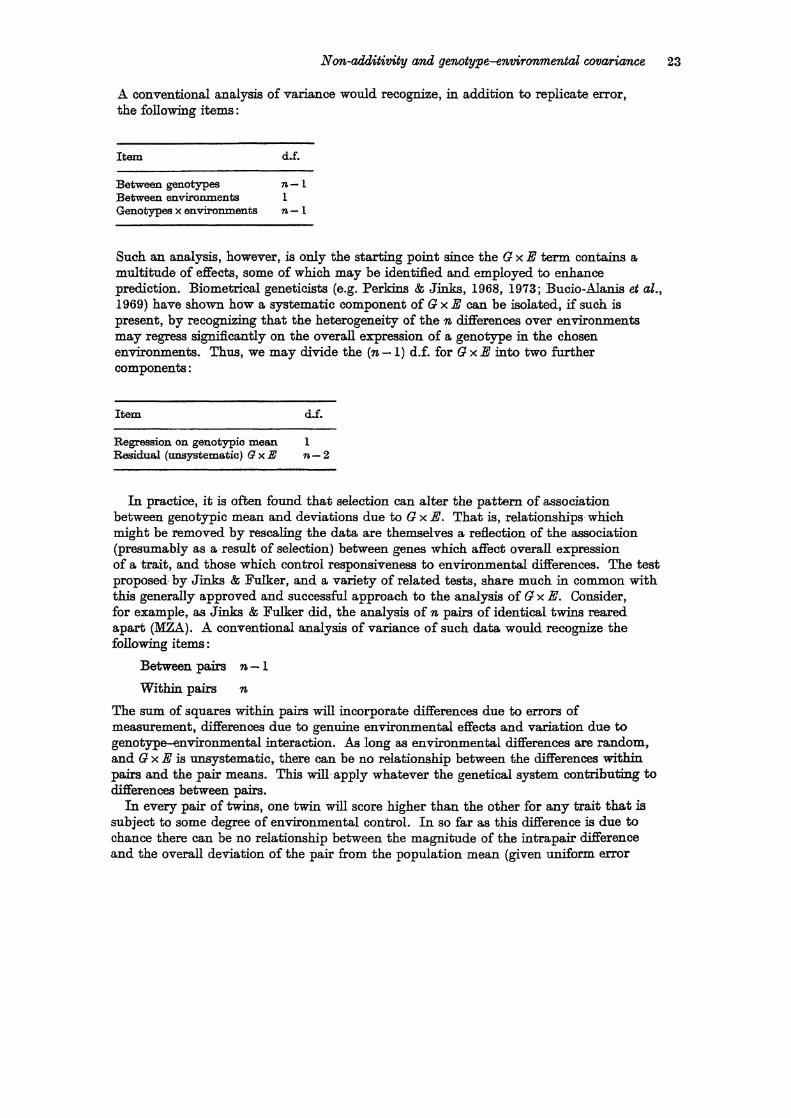
Non-additivity and genotyper-environmental covariance 23

A conventional analysis of variance would recognize, in addition to replicate error, the following items:

Item d.f.

Between genotypes n- 1 Between environments 1 Genotypes x environments n - 1

Such an analysis, however, is only the starting point since the G x E term contains a multitude of effects, some of which may be identified and employed to enhance prediction. Biometrical geneticists (e.g. Perkins & Jinks, 1968, 1973; Bucio-Alanis et at., 1969) have shown how a systematic component of G x E can be isolated, if such is present, by recognizing that the heterogeneity of the 11, differences over environments may regress significantly on the overall expression of a genotype in the chosen environments. Thus, we may divide the (11,-1) d.f. for G x E into two further components :

Item d£.

Regression on genotypic mean 1 Residual (unsystematic) (} x E n - 2

In practice, it is often found that selection can alter the pattern of association between genotypic mean and deviations due to G x E. That is, relationships which might be removed by rescaling the data are themselves a reflection of the association (presumably as a result of selection) between genes which affect overall expression of a trait, and those which control responsiveness to environmental differences. The test proposed· by Jinks & Fulker, and a variety of related tests, share much in common with this generally approved and successful approach to the analysis of G x E. Consider, for example, as Jinks & Fulker did, the analysis of 11, pairs of identical twins reared apart (MZA). A conventional analysis of variance of such data would recognize the following items:

Between pairs 11, - 1

Within pairs 11,

The sum of squares within pairs will incorporate differences due to errors of measurement, differences due to genuine environmental effects and variation due to genotype-environmental interaction. As long as environmental differences are random, and G x E is unsystematic, there can be no relationship between the differences within pairs and the pair means. This will apply whatever the genetical system contributing to differences between pairs.

In every pair of twins, one twin will score higher than the other for any trait that is subject to some degree of environmental control. In so far as this difference is due to chance there can be no relationship between the magnitude of the intrapair difference and the overall deviation of the pair from the population mean (given uniform error

24 L. J. Eave8, Krystyna La8t, N. G. Marlin and J. L. Jinka

variance throughout the scale). The difference in score, however, implies that relative to one another, one twin has experienced a superior environment and the other an inferior environment. We may use the difference in scores within a pa.ir as an indicator (of uncertain realia.bility) of the difference between superior and inferior environments, and we can ask: 'Does the difference between the effect of superior and inferior environments depend on the genotype of the individuals concemed1'. Jinks & Fulker approach the question through a regression analysis of the absolute intrapair differences. The uncorrected sum of squares of the absolute differences is equal to the within-pair sum of squares of the conventional analysis of variance of the paired scores. Implicit in the regression analysis is the following partition of this sum of squares:

Item d.f.

Correction term ('superior vs. inferior environment') 1 Linear regression (systematio G x E) on pair means 1 Residual (non-linear systematio GxE, unsystematio GxE, etc.) n-2

The linear regression on pair means will be significant if there is G x E such that the genes which contribute to sensitivity to the environment are correlated in distribution or action with those affecting overall performance. We may conceive of such interactions in physiological or social terms. Thus, for example, individuals who score high on a trait may be more stable developmentally than low scorers. That is, the effect of the same envitonmentaI influences changes systematically With genotype. Alternatively, individuals who on average manifest high scores may find themselves in more variable environments because there is no consistent policy towards the treatment of such individuals (Eaves, 1970).

We may illustrate the approach by reference once more to the often publicized and much criticized data. of Burt (1966), described in section 6 • .2(c) above, which comprises IQ scores of 53 pairs of MZ twins. One member of each pair was reared by his natural parents and the other in a foster home. There is no detectable correlation between indices of SES of the natural and foster homes.

The basic analysis of variance of these data is as follows:

Item d.f. ss MS

Between pairs 52 21 817·60 4:19'57 Within pairs 53 . 1455·00 27·45

Following the argument of Jinks & Fulker (1970) we may further analyse the variation within pairs as follows:

% of total SS Item d.f. SS MS within pairs

'Superior vs. inferior environment' 1 942·04 94:2·04: 64·7 Regression on mean 1 2·09 2·09 0·1 Residual 51 510·87 10·02 35·1 Total 53 1455·00 99·9

The comparison of 'superior and inferior' environments, based as it is upon an examination of the twins' scores, is likely to be an overestimate of the 'true' overall difference between the twins' environments and is included merely to indicate the structure of the a.na.lysis. The residual sum of squares is a guide to the relative importance of heterogeneity of superior and inferior environments over pairs and unsystematic G x ]jJ effects.

If we assume, for the moment, that the usual tests of significance are appropriate here, we find that the regression does not account for a significant proportion of the variation in environmental differences around their overall mean. That is, the data. give us no reason to suppose that systematic G x ]jJ effects need to be taken into account when making predictions on the basis of IQ tests.

We may wonder whether the test of significance is appropriate given that we decide from the data. which twin received which environment. Dr M.. J. Kearsey of our Department kindly made available to us a computer pa.cka.ge he had developed for the simulation of various aspects of polygenic inheritance and experimental design in biometrica.1 genetics. Genetica.1 variation is simulated on the assumption of ten loci in linkage equilibrium. The dominance effects of the loci and the frequencies of their alleles can be varied. Random mating is simulated. Environmental variation is simulated by random processes, either specific to individuals or common to families. .As part of a programme of computer simulation (Martin, 1976), we generated 400 sets of 500 MZ twin pairs. This comprised 25 replications of each of eight different populations, differing in the degree of genetic determination, the amount of dominance and the relative importance of environmental differences between families. No systematic G x E was specified in the model used to genera.te the data.. The regression analysis described above was used for the 400 sets of twins and in only 14 of the simulations (3l per cent) was a significant linear component of regression detected at the 5 per cent level. The fact·that·this is close to the expected proportion of significant results, given that the null hypothesis is true, ~gests that the test of significance we employ is not seriously misleading. These simulations also confirm the model of Jinks & Fulker which implies that in the absence of G x E there is expected to be no significant relationship between sum and diff~ce for monozygotic twins reared apart.

The power of the te8t for ay8terna;tie G x E. Although, as we shall show, small amounts of unsystematic G x]jJ are difficult to detect, our experience has shown that this is not the case for systematic types of G x E. In an a.na.lysis of a variety of behavioural traits involving quite small samples of MZ twins reared together, Martin (1976) showed that systematic non-additive effects, accounting for no more than 5 per cent of the total variation within MZ pairs, could be detected at the 5 per cent level with only 95 pairs of twins. Even with samples as small as 39 pairs he was able to detect non-additive effects accounting for not more than 12 per cent of the variation within pairs.

So far we have restricted our consideration of GI x ]jJ to systematic linear effects. There is no particular reason why such effects should be linearly related to the genotypic mean. Indeed, there are many situations in which we might find significant non-linear trends. Society may react in a uniform way to extreme deviations on either side of the population mean. This would produce a pattern of G x E which shows greater environmental variation in the middle of the sca.1e than at either end. In practice, this kind of interaction is common in psychometric data. because of floor and ceiling effects. In Burt's data. there is little suggestion of such interaction, but many personality sca.1es show apparent interactions of this type when raw scores are used. In a recent twin study, responses of 316 MZ twins were obtained to 74 items relating to neuroticism.

26 L. J. Eal1es, Kryatyna Last, N. G. Martin and. J. L. Jink8

When neuroticism scores were computed simply by counting the number of 'neurotic' responses made by each individual, a highly significant quadratic relationship was obtained, with pah-s at the tails showing much smaller differences within pairs than those in the middle of the range.

Ge:notype-enmronmentaZ interaction aM 'seale'. Such interaction could be explained in terms of the properties of the scale, since it is well known that the error variance of scores of this type depends on the subject's propensity to endorse dichotomous items in a given direction. In order to test the hypothesis that all the G x Jj] interaction could be attributed to the heteroscedasticity created by a choice of scale, we attempted to remove the interaction by an angular transformation of the proportional scores. Indeed, we found that the transformed scale showed no evidence of any systematic non-additivity of any kind. In a similar study of psychoticism, Eaves & Eysenck (1977) showed that any non-additivity could be removed by a simple transformation which assumed that the psychotic responses of individuals to items of the EPQ were randomly distributed OT'er the items of the P scale with a frequency for each subject which appeared to be under genetical control. Last (1976) has analysed raw scores relating to various aspects of cognitive abilities for black and white twins in the-US. She found similar interactions to those found for personality scores, and concluded that sexes and races might differ superficially in their apparent sensitivity to differences in the environment, but that such apparent differences can largely be attributed to the fact that threshold effects play a more significant role in some groups than others.

These findings point to a dilemma in the analysis of certain behavioural data. Either we accept .the scale that is used for convenience and tolerate the non-additivity generated by such scales, or we attempt to produce a scale which is free of such interaction but which will inevitably be measuring a somewhat different trait. These scales permit a more reliable analysis, produce tidier cOnclusions and have much to commend them for predicti"\?"e purposes because the problem of heteroscedasticity has been overcome. The search:for a scale which is more appealing from the psychological standpoint is not, however, without its problems from the biometrical-genetical view.

We may illustrate the problem by brief reference to an attempt we made to measure_ -neuroticism on a scale which had greater behavioural relevance. We took the responses of 1174 twins of both sexes (including our 316 MZ twin pah-s) to the 74 neuroticism items of ourexperiroental questionnaire and subjected these to analysis in terms of the two- _ parameter logistic model of Birnbaum described by him in Lord & Novick (1968). We estiinated the item parameters and the latent trait scores for all the subjects in the -study. In spite of the fact that we liad a fairly large number of items related to neuroticism, at least by comparison with those in the N scales of the EPQ and EPI, the amount of information (i.e: the inverse of the score variance) computed for different scores on the latent trait model showed a very substantial reduction as scores became more extreme. In fact, information was mmrnal (or the variance of scores was smallest) for scores approximately 1 S.D. from the zero point of the scale. This is to be expected for a collection of items which have presumably been selected at some time or other for the discrimination of relatively extreme neurotics from the rest of the population. -

Whilst such a model makes psychological sense, its consequences for any genetical analysis are quite extreme. The relationship between sums and differences for the latent trait scores shows the marked U-shaped relationship to be expected from the fact that the amount of information about a subject is so greatly reduced towards the extremes of the distribution. Of all the possible ways of summarizing the information in a set of

responses to the same questionnaire data, that which is most appealing for psychometric reasons is that which requires the most complicated explanation of the pattern of individual differences. Indeed, none of the simpler additive models could account for the variation in neuroticism as it was measured by a logistic model for the subjects' responses. In fact, the genotype-environmental interaction imparted to the data an apparent consistency with a mechanism involving some kind of sex linkage or sex limitation, to judge from the differences in mean and variance between the sexes. A similar result has been claimed by others (e.g. Bock & Kolakowski, 1973) for variation in spatial ability when subjects' scores have been assessed. on the basis of a similar psychometric approach. A recent study of parent offspring similarity by DeFries et at. (1976) does not support the hypothesis of sex linkage for spatial visualiza.tion and leads us to wonder whether scalar properties could not explain the earlier finding.

The important point to notice about this discussion is that three different methods of scaling the same behavioural data yield quite different conclusions about the form of G x E (and presumably also about the genetic architecture). The raw scores yield a scale on which individuals at the extremes are apparently less sensitive to the environment, the angular transformation yields a scale on which environmental factors have a uniform effect over the whole range, and the logistic model yields a scale on which the influence of the environment appears to be much greater in the tails. None of these scales is 'right', they all employ the same information. As far as a genetical analysis is concerned a change of scale amounts to Stressing the consequences of some gene substitutions or environmental· influences at the expense of others. In the end, a satisfactory scale is one which yields the most effective general predictions.

There is no reason to suppose that all scales show such striking problems of non-additivity. In an analysis of a social attitude questionnaire consisting of 68 trichotomous items scored 1, 2, 3 we found that a general factor corresponding to 'conservatism' produced scores for the 316 MZ twin pairs which showed virtually no evidence of non-additive effects of the kind we have discussed so far. Out of the 14 ability scales studied by Last (1976), six showed evidence of systematic G x E in their raw form. Often simple transformations were·insufficient to remove such non-additive effects. Martin (1976) has analysed the raw scores of 134 MZ twins pairs from a; variety of personality and attitude factors and concluded that five out of ten scales showed some form of systematic non-additivity which could be removed' by. suitable. ~ormation. In a reanalysis of certain data on 40 MZ pairs from the Michigan twin study (Vandenberg, 1962), Eaves (1970) found systematic linear interactions for 12 out of 36 traits.covering a.wide range of behavioural measurement.

Jinks & Folker (1970) considered the consequences of G x E for the rel8.tionShips between pair means and absolute differences for MZ twins. They observe that twins reared.apart will provide the best basis for detection of G x E for two reasons:

(1) All G x E involving interaction of genetical differences with environmental differences within and between families will be confounded with differences within pairs, whereas only genetical differences will contribute to differences between pairs, given random placement. Such a set of twins, therefore, means we can study the components of all kinds of G x E in relation to genetical differences in the population. IT the twins are reared together, however, any interaction of genetical differences with between-family environmental effects is confounded with the corresponding genetical and environmental effects. This means that MZ twins reared together can only be used to detect systematic components of interaction between genes and intrafamily environmental effects.

(2) The use of MZA will ensure, as far as possible, that interaction between different sources of environmental variation will contribute only to differences within pairs and be

28 L. J. lCa'lJe8, Kryslyna Lut, N. G. Martin and J. L. Jinlc8

uncorreIa.ted with genetical effects. Interaction of this type would result if there were cultural differences between families such that certain pa.rents tended to treat all their own children uniformly whilst other parents treated their children individually.

Wh.a.tever the family structure, interactions which involve differences within families will contribute to variation within families, but if there is systematic interaction between cultural effects a.nd treatment differences within families (lC'I. x lC,J these will contribute, as Jinks & Fulker have shown, to the covariance of means a.nd intrapair absolute differences for MZT. In order to interpret a relationship between means a.nd differences for MZT as G x lC we have to be fairly sure that there is no major contribution from cultural effects to differences between pairs. Ideally such a question is best answered by data on fostered individuals, although the approach of model :fitting to statistics on relatives reared together ca.n give some indication of the likely significa.nce of cultural differences between families (see e.g. Eaves & Eysenck, 1977).

7.2. Detecting 8'f/8tematic genetical rum-additi'Vity

Our test of G x lC is effectively a test based on third-degree statistics since we are looking at the covariance between mea.ns and a measure of variation, in this case the standa.rd error, within families. In general, we would expect the effects of other systematic non-additive effects· to be detectable with third-degree statistics. In any study of individUal differenCes there is a variety of such statistics that ca.n be calculated which may shed additional light on sources of non-additive varia.tion: Some,but not all, o(these possibilities were considered by Jinks & Fulker (1970). For example, they noted that the' a.verige Skewness within sibling families could detect directional domina.nce in. the, a91j16nce of G x lC. ,Fisher et aI. (1932) showed, for the case of eqUal allele :frequencies, that a variety of third-degree statistics could provide information about the direction, of dominance in the absence of other sO~ces of systematic non-additivity. Thus the population skewness was expected to differ from zero in the presence of directional dominance and the means and variances of sibships were expected to cova.ry. As the number of loci increases, the contribution of dominance to third-degree statistics is reduced. In natural populations, for which allele :frequencies are not expected to be equal, any systematic inequality of allele frequencies (i.e. any general tendency for increasing alleles to be more or less frequent than decreasing alleles) will contribute to the same third-degree statistics, even when gene action is additive. Simi1a.rly, any general systematic epistatic component, such as that introduced because of a threshold effect on gene substitution, will result in detectable skewness or covariance of family means and variances.

The power of the test. Martin (1976) used the simulation package developed by Kea.rsey and described in section 7.1 to test the practical utility of these approaches to the detection of systematic genetical effects. From a variety of such populations Martin generated 25 replicate sets of 500 pairs of siblings a.nd tested for population skewness and for the regression of absolute intrapair differences on pair means. A sample size of 500 pairs was chosen as one which might reasonably be expected in practice.

Some of the salient conclusions for this study are given in Table 6. This table includes only those simulations in which the allele frequencies were 0·5 at every locus. In such cases, a.ny skewness or covariance of pair means and variances is attributable to directional dominance. We see that the power of the test of directional dominance, for the given sample size, is quite good (80 per cent with 500 pairs) provided that the broad heritability is high. As we might expect, however, the power of the test fa.lls

quite rapidly as the contribution of environmental variation increases. Eaves (1972) obtained similar results relating to the detection of dominance by model fitting to second-degree statistics. In that case, however, the emphasis was on the detection of dominance variation, irrespective of any directional component. .As we might expect, a weaker null hypothesis will be accompanied. by a reduction of our ability to reject such a null hypothesis given that it is actually false. Thus, we find that if we do not specify the direction of dominance, but are merely concerned to detect variation due to dominance, considerably larger sample sizes are needed.

Table 6. The power of detection (5 per cent level) of directional dominance with third-degree statistics from simulated twin studies using 25 replicationst

Cultural Expected Observed Observed h&2 hId effects skewness skewness power(%)

009 1·0 Absent -0·31 -0031 96 Present -0·31 -0-30 100

0·5 Absent -0·24 -0·24 84 Present -0·24 -0-22 80

0·5 1·0 Absent -0·13 -0·14 48 Present -0·13 -0·13 32

0·0 Absent -0·10 -0·09 12 Present -0·10 -0·09 16

t ~I is the broad heritability; hId is the ratio of dominance deviations to additive effects.

Martin (1976) simulated data on monozygotic twins in addition to those on siblings for the same set of simulated populations. After summarizing the data by analysis of variance within and between pairs, estim.ates·of additive, dominance and· environmental variation were obtained with their standard errors. The power of the test of dominance variation, based on 25 replicates of 500 MZ and 500 sibling pairs, was found empirically to be 80 per cent for the population with complete dominance and a broad heritability of 0·9, but when the dominance ratio was reduced to 0·5 the power was only 28 per cent. For populations in which the broad heritability was 0·5 the power of the test of dominance was virtually zero with these sample sizes. These findings confirm those obtained by Eaves (1972) for the expected power of tests of dominance by model fitting to second-degree statistics.

8. Detecting unsystematic G x E and genotype-environmental covariation

The theoretical investigation of Last (1976) is too extensive to consider in all its details, but we abstract the features of her approach which are most salient in our context. Starting with the experimental design we have introduced, she produced expected values for the various second-degree statistics obtained from such a study for a variety of systems of causation. Then, using the approach of weighted least squares to obtain the minimum variance unbiased estimates, she determined the total sample size necessary to be 95 per cent certain of detecting given effects at the 5 per cent level, given that the correct model was fitted. The general method she used was that of Eaves (1972). However, she went further to investigate the biases introduced into estimates of the parameters of various inappropriate models, given that such models were mistakenly adopted as provisional explanations for the observed pattern of

30 L. J. Eaves, Kryatyna we, N. G. Martin and J. L. Jinlc8

individual differences. Also, by loomg at the significance of the residuals after fitting inappropriate models she was further able to judge the likelihood of detecting the mistake. The models employed covered many situations involving various degrees of non additivity and non-independence of genetical and environmental effects.

The experimental design of section 5.2(a) was adopted to allow all the effects in which we were interested to be detected, in principle, within the framework of linear model fitting. Many effects, for example, those of assortative mating and cultural transmission, make contributions to other second-degree statistics which are formulated more parsimoniously in terms of a non-linear model. The application of weighted least squares to the testing of such models for real data is quite possible (see e.g. Eaves, 1975), but the approach is tedious for simulation studies such as these.

8.1. Genotype-enmronment interaction

To help the reader grasp the method we give one example in more detail before outlining the results of others. Consider a randomly mating population in which there is additive gene action and environmental variation within and between families. The environmental differences between families are independent of genetical differences but the two sources of variation interact producing variation due to the interaction of additive genetical differences with environmental differences between families. The model for the population variance may then be written as

up 2 = tDR+El +Ea+t(DREa)·

As previously, the term DREa does not denote a multiple, but indicates the interaction . of additive genetical differences with environmental differences. between families.

. In general, the genes and environments which contribute to DJlEa need not also contribute to DR and Ea. but if they do contribute in any systematic way to these parameters, then their effecf;:s could be detected with some of the methods considered above.

(a) Generating the 'data'. Expectations for the 11 statistics of our experimental study were written in terms of these parameters. Parameters defining interactions involving within-family environmental differences were not included since these are inevitably confounded with E1• The expectations are given in Table 7.

In order to generate numerical expectations for the 11 statistics we must specify values for the four parameters. These are arbitrary, but some sets of values are more consistent with the existing body of information about the causes of continuous variation. Thus, it seems reasonable to suppose that about half of the total variation for a trait is due to environmental differences. So for convenience, fixing up'l at 225 we have

El +Ea = 225/2 = 112·5.

The contributions of El and Ea are determined empirically for any real set of data. We shall generate expectations on the assumption that El = Ea = 56·25. The remaining 50 per cent of the variance can be assigned to the additive effects of genes and their interaction with environmental differences between families; that is, iDR+tDREs = 112·5. We now must decide the relative magnitudes of DR and DREs to be incorporated in our simulations. In experimental organisms it is seldom found that more than 20 per cent of the variation between genotypes and treatments can be attributed to G x E, so we choose a value of DRE." satisfying tDREs = 225/5 = 45. Thus, we give the value 90

Non-additivity ani/, ge:notype-e:n:oironmental covariance 31

to DRE2 and to DR we give the value (1l2·5-45) x 2 = 135. The vector of parameters used to generate the expected statistics, for the purposes of the present example, is thus:

( D:~2) _ ( 1::::).

E2 56·25

El 56·25

The expected statistics are obtained by post-multiplying the model matrix of Ta.ble 7 by this vector of estimates. For example, the expected. mean square between MZ pairs reared together is

MSbMZT = DR+DRE2+El +2E2

= 135·00 + 90·00 + 56· 25 + 112·50

= 393·75.

The full vector of expected mean squares, given our parameter values, is given in the same table.

Table 7. A simple model involving genotype-environmental interactions used for simulation

Mean squa.re DR El E, DRE2

Between MZT 1 1 2 1 WithinMZT 1 Between DZT f 1 2 i Within DZT t 1 t BetweenMZA 1 1 I t WithinMZA' I' I i BetweenDZA ! 1 1 i WithinDZA ! 1 1 i Between UT t 1 2 t Within UT t 1 ! Singletons ! 1 1 !

(b) The 'estimates' ani/, their expected variances. Now we can do several useful computations. For example, we may proceed as if we were fitting the correct model (Le. the model in Table 7) and obtain expected values for the variances and covanances of the four parameters. The covariance matrix of the estimates would be

Z = (A'WA)-l,

where A is the model matrix (Table 7) and the diagonal elements of Ware the reciprocals of the expected variances of the observed mean squares, i.e.

W,i = nJ2szi 2

where the ni are the d.f. of the mean squares Zi' We ha.ve made one approximation for simplicity, by assuming all the ni are equal. In fact, the d.f. between pairs should be one less than those within pairs. The simp1i:fication makes the repetition of the calculations easier, and has a trivial effect on the outcome.

32 L. J. Eaves, Kry8tyna LaBt, N. G. Mamn and, J. L. Jinlc8

The diagonal elements ofW are: (0·000322, 0·015802, 0·000584, 0·002016, 0·000439,0·003951, 0·000747, 0·001367, 0·000632, 0·001756, 0·000988). Since the mean squares are independent, a.ll off-diagonal elements are zero.

The covariance matrix is

DB DBES IDa

DR ( 1409-6177 -1304-6148 61-3961

DBES -1304·6148,2841-1789 -635-0964

JiJs 61-3961 -635-0964 321·5570

El 3-8203 -156-5776 20-4463

El

3-8203 ) -156-5776 _

20-4463

59-3642

The estimates (8) and their standard errors (Gs) are thus:

( ~:Es ) ( 1:~:: ) ( :~::: )_ Es 56-25 17-93

El 56-25 7-70

e Gs

We ma.y divide each element of 8 by its corresponding as to give a vector of normal deviates which are the expected values of 8,,ju8{, for samples of this size and structure from populations in which individual differences are determined by the effects specified in the model. This vector is

'( 3-60 ) 1-69 c=

3-14

7-30

In practice we would perform a two-tailed test of significance because, even though the components of variance are expected to be positive if the model is appropriate, significant negative estimates of parameters would be taken as a clear indication that some other model is more appropriate. Thus, there are two criteria of the adequacy of a particular model. The first is the purely statistical criterion of whether the residuals are too large to be explained by chance alone. The second criterion is whether the estimates we obtain are consistent with biological theory_ We shall see in due course that biologically nonsensical answers are often as clear a guide to the inadequacy of a model as the significance of residual effects.

(c) The power of the tests of G x E. The expected values of the normal deviate show that we would frequently expect to detect DR' El and E'}. as effects significantly different from zero, but that we would fail to detect G x E in a large number of cases_ This statement may be quantified by calculating the power of each of the tests; that is, we can determine the proportion of studies of this size and structure in which we would reject at the 5 per cent level the four separate null hypotheses that DR' DREs, Es and El were zero, given that the popula.tion parameters take the values used in generating the expected mean squares_

The power of the two-tailed test at the 5 per cent level is equal to the area under the normal curve having zero mean and unit variance between limits 1-96-c and infinity,

where c denotes the expected value of 8/0'0 for a particular pa.ra.meter. The values of 1·96-c corresponding to the four parameters are -1·64,0-27, -1· IS, -5·34 respectively, giving for the power of each of the tests 0'9495, 0-3936, 0'SS10, 1·0000. That is, tests of the main effects of genes and environment are very powerful, but a study involving 1100 d.f. would only be 39 per cent certain of detecting G x JjJ involving environmental differences between families, given that such interaction accounted for as much as 20 per cent of the total variance. Obviously, the power of the test would be substantia.lly increased if the contribution of G x JjJ were larger, but we have chosen to examine the consequences of a relatively sma.ll amount of G x JjJ because that seems to be typical of real data e.xa.mined to date.

The power calcula.tions may be extended, following Eaves (1972), to determine the sample size which would be necessary to ensure greater power, say 95 per cent, for the detection of G x E. For this purpose, we require the sample size which would produce an expected value of 1·96+1·65 = 3·61 for 8/0'0' We already know that the amount of GxID in our hypothetical population produces 8/0'0 = 1·69 for a total d.f. of 1100. The value of 9/0'0 increases as the square root of the sample size, so writing k for the ratio of the required sample size to that used in our study we get ~lc = 3'61/1'69, giving k = 4·5629. The sample size required to give· 95 per cent certainty of detecting G x JjJ at the 5 per cent level is thus 1100k, or 5019. This fairly prohibitive requirement suggests that G x ID which is not systematically related to genetical or environmental deviations (and therefore undetectable by other methods) is unlikely to be detected by fitting linear models to second-degree statistics unless the contribution of G x E is much larger in man than is usually the case in other organisms.

(d) .A88e88ing the biaa in estimates. If we proceed on the (false) assumption that G x E was absent biases would be introduced into 'the estimates of the main effects. The effect of these biases on subsequent inferences can be assessed accurately. We consider the simplest possibility which is likely to occur in practice, namely, the fitting of a model involving DB' El and ID~ to statistics derived from a population in which there is G x ID due to DBIDS in addition to the three main effects.

Starting with the expected mean squares generated in the previous example, we attempted to fit three parameters, DB' IDl and IDs, by an iterative weighted least squares procedure, in which the expected values generated by fitting the model are used to produce new weights for each iteration. This is the procedure adopted in the analysis of actual data (e.g. Eaves & Eysenck, 1975).

The estimates are given by (A 'W A)-l A 'Wx where W is evaluated for the parameter estimates which mjnimize the weighted squared deviations of 'observed' from predicted mean squares. The contribution of the 'true' parameters to these estimates may be obtained from the rows of (A' W A)-l A' WB where B represents the 'true' model for the observed statistics.

For the case in which we fit only DB' IDl and IDs to the population in which DR' IDl • IDs and DBID'J contribute to variation we find

.' 0.4567) ( ~: ) • 0·2304 .

IDl 1 0·0714 DREs

As we might expect, the estimate of IDl is virtually unbiased, having only O·0714DB ID'J as bias. The variances of DB and ID2• however, show a somewhat greater bias, DB

3

34 L. J. Eaves, Krystyn.o, Last, N. G. Martin and J. L.Jinlca

containing 0'4567DB E s and Es containing 0·2304DB E s' In this particular hypotheticaJ' example, therefore, the estimate of DB is 176·10 compared with a true value of 135, and the estimate of Es is- 76·99 compared with a true value of 56·25. Hence, G x E leads to a- bias which overestimates both genetical and cultural effects if the contribution of G x E is ignored in fitting the model. The geneticaJ component of the total variance is, however, iDB not DB' and the bias in IDB is very nearly equal to that in R2. That is, G x E biases equa.lly our estimates of the contributions of genetical differences and environmental differences between families to the total variation.

Thus, although G x E may pass undetected. if it is completely unsystematic, and although G x E will bias our estimates of genetical and environmental variance in such circumstances, it will none the less bias equaJIy our estimates of DR and Es in the same direction. In the light of this discussion, therefore, it seems appropriate to compute the estimate of the (narrow) heritability which would be obtained if a simple model were fitted in which the contribution- of G x E was m.ista.kenly ignored, and to compare the value with that computed from the true parameter values. We do this, not because we believe a knowledge of 'heritability' is fundamental to the problem of individual differences, but because certain authors (e.g. Moran, 1973; Layzer, 1974; Feldman & Lewontin, 1975) have focused much of their criticism of the analysis of human behaviour on estimates of 'heritability'. In writing an expression for the 'true' heritability, given G x E, we include any variation due to G x E in the denominator only. Thus,

hS == IDBi(!DB+E1 +Es+!DRE2) == 0·30.

If, however, only DB' El and Es are fitted, then the heritability obtained is

h2 == !J)Bi(!J)B+11 +:e~ == 0·3867.

That is, proceeding with the eStimation of heritability on the assumption of no G x E is likely to lead to an overestima.te of the true contribution of additive genetic variance to individual differences, when the estimate is based on the constellation of relatives we have considered here. Caution is advised, however, since this is not a general rule. Genotype-environmental interaction could lead to underestimation of additive genetiCal variance from transgenerational data (e.g. parent--offspring covariances), and the precise nature of any bias would have to be determined for each specific situation. Indeed, one drawback of a.ll calculations of this kind is their lack of generality. We can merely explore the weaknesses of particular studies under a selected range of circumstances. -

Although we sometimes include G x E with the non-heritable agencies, for predictive purposes we should recognize that the existence of G x E mdicates that sensitivity to the environment is to a greater or lesser degree under geneticaJ control. This enables expectations for G x E to be written in terms of gene effects. Furthermore, the existence of G x E indicates that sensitivity to the environment is potentially subject to the influence of selection. To affirm, as many have done, that the certainty of genotype­environmental interactions undermines genetical analysis, is both to exaggerate their significance relative to the overall variation in a population and to miss their potential biological significance.

8.2. GtnOtype-environmentaJ, C01J(],Mnce Last (1976) conducted similar studies in relation to many other effects, including those of assortative- mating, dominance and genotype-environment covariance. We consider some of her results relating to the detection of genotype-environment covariance.

Non-additivity and genotype-environmental covariance

(a) Sibling effects. Using the model developed by Eaves (1976a), Last investigated the detection of environmental variation and genotype-environmental covariation due to the effect of one sibling on another. A simple system was considered in which all gene effects were additive and in which the only common environmental component was that due to the genetical covariance between members of a twin (or sibling) pair. Thetotal variance of singletons was thus specified as o-s2 = !DR+E1, there being no variation due to sibling effects in individuals reared alone. Following the procedure previously adopted, El was equated to tDR and o-s2 was arbitrarily fixed at 225, giving El = 112·5 and DR = 225. In order to specify the sibling effects, we have to provide values for DR (the 'genetic environmental' variance due to sibling effects) and Dit (the genotype­environmental covariance parameter).

Table 8. A simplified model for sibling effects used in simulation

Parameter

Mean square DR Dii D' B El

BetweenMZT 1 1 2 1 WithinMZT 1 BetweenDZT t ! l-i 1 Within DZT t t --i 1 BetweenMZA 1 1 WithinMZA 1 BetweenDZA ! 1 WithinDZA t 1 Between UT t t 1 1 Within UT t t -1 1 Singletons t t 1 1

The model, given in Table 8, shows that the contributions of environmental variance, specified by DR' and of Cov GE, specified by Dit> depend on the degree of relationship between members of the pairs contributing to a particular statistic. Thus, although there is an explicit interpretation of DR' DR and DR' their relative contributions to particular statistics change. This means, further, that any estimate of Pge depends on the degree of relationship, and on the relative contribution of El and DR to the total variance. It is small wonder, therefore, that previous attempts to specify CovGE have foundered at the outset.

For the purposes of simulation, Last assumed that Dii = !DR ; that is, the environmental variance due to sibling effects was assumed to be half that due to E1.

The only remaining difficulty was the specification of DR' This parameter is, in effect, a measure of the degree of pleiotropy or association between the direct effects of genes on an individual's phenotype and their indirect effect, through the environment, on the performance of a sibling. In this sense, and in this sense only, it is meaningful to define, and solely for the purpose of these simulations, that Pae = DitN(DRDR).

When the allele :frequencies are equal at every locus contributing either to DR or DR' and when all loci have consistent and equal effects (see Eaves & Gale, 1974, for a definition of consistency in this context), then Pge is the proportion of loci which contribut both to DR and DR' That is, Pge is the proportion of loci having both direct effects on the phenotype, and indirect effects on the phenotype of siblings. Last chose to work

36 L. J. Ea'Ue8, Kry8tyna Laat, N. G. Martin and J. L. Jinks

with Pue == 0·5. The values employed in generating her statistics, therefore, were DB == 112·5 and DB == 79·5495.

With the sample structure she had assumed (1100 d.f.), Last was able to derive values for the powers of the tests of the four parameters, DR' DB' DB and lOt. These values were 1·00, 0·99, 0·67 and 1·00 respectively. Thus, we see that the present design is quite powerful for detecting sibling effects, especially when these covary with the direct effects of genetical differences. The fact that the test of DB is more powerful than that of DB arises because the test of DB depends merely on a comparison between the total variances of individuals reared as pairs and singletons, whereas the significance of DR depends on a very precise pattern of expectations which involve the individual mean squares as well as the total variances.

By considering the case in which DR is positive we have assumed a cooperative situation in which a high performance of one sibling enhances the performance of another. We must also consider the possibility of a competitive situation in which the success of one sibling is achieved at the cost of the other. Last simulated competition by using the same parameters as the cooperative model, except that DB was replaced by a . negative value, - 79·5495. The values obtained for the powers of the four tests of DR' DR' DB and El were now 1·00, 0'95, 0·57 and 1·00, suggesting that the detection of competitive effects is no less viable than the detection of COoperation. Indeed, we suspect that competition may be easier to detect than coopera.tion in experimental designs which lack individuals reared as singletons. _ .

(b) Oultural tranamiBBion. Finally, we examine the detection of genotype-environment covariation arising as a result of the cultural impact of parents on their offspring. Eaves (1976b) has shown how the empirical components 109 and COVUgeg may be represented in terms of a. cultural transmission model in which the phenotypic variation between parents is p~:i:petuated culturally as well as genetically in the offspring generation. Using b to denote the regression of the family environment of an offspring on the phenotype of his parents, it can be shown, in a randomly mating population that

and

Any common environmental effects of a non-cultural kind are excluded from this formulation of the model, but need not be excluded in principle. The magnitude of 109 and CoVugeg depend on the size of !DR' but Es is further increased by the contribution of dominance and random environmental factors. We consider one of the simulation studies conducted by Last (1976) which assumed that, in the absence of cultural transmission and given complete additivity, !DR = El == 112'5, i.e. that the heritability of the trait would be 0·5 in the absence of cultural effects. Assuming that cultural transmission was entirely responsible for any common environmental effects, it is possible to calculate expected values of lOs and 2 Cov gg es for a given b. Last considered the consequences of b == 0·1 and b == 0·25. For b == 0'1, we get 109 == 6·76 and 2CovUseg = 50·00. These values may be compared with those of 61·61 and 150·00 for Eg and 2 CovUseg when b == 0·25, given random mating, additive gene action and !DR/(!DR+El ) = 0·5.

N on-additivity and, genotype-environmental COfJanance 37

Strictly speaking, since only one new parameter, b, is required to specify the consequences of cultural transmission for Es and Covg,~ it would be appropriate to employ the more powerful approach of non-linear weighted least squares (e.g. Eaves, 1975) to estimate b, DR and E I , but we choose to continue the approach adopted 80 far and estimate four parameters E" Covg,~, EI and DR' This is sufficient for our purpose, but does not enforce the constraint upon E, and Covg,e, which is implied in the model of cultural transmission. We may find, however, that real data do not fit exactly into the mould of our equilibrium model, so the restraint may need to be relaxed anyway in practice. From this point of view, the approach we adopt here may be more generaJIy applicable.

For the case of b = 0'1, the powers of the tests of the parameters were found to be 1·00, 0·39, 0·76 and 1·00 for DR' Es, Covg,es and EI respectively . .As b or h' increase, of course, the tests become much more powerful. Thus, for b = 0·25 the powers become 1·00, 0'99, 0·99 and 1·00. If the contribution of IDR is increased rela.tive to that of E I ,

so that IDRilDR+EI = 0·9 (i.e. DR = 405 and El = 1l·25), then for b = 0·1, we obtain E, = 10·33 and 2 Covgses = 90. For b = 0·25, we obtain E" = 98·04 and 2Covg,e" = 270. The power of the test for E, is 0'87, when b = 0·1, and 1·00 when b = 0·25. The powers of the tests of genotype-environmental covariance are 0·93 and 1·00 for b = 0·1 and 0'25, respectively.

We give somewhat fuller results for the cultural transmission model because of the potentia.! theoretical significance of Cov g" e2• The power of the test of Cov g, ~ is found to be reasonable (>0·75) for this sample structure when b~O'1 and when IDa~El' In terms of the more usual models for genotype-environmenta.l correla.tion, these parameter values coincide with overall genotype-environmental correlations of 0·31 (for b = 0·1, IDa = E1) and 0·65 (for b = 0'25, tDR = E I ).

We can obtain the linear combination of the observed statistics which yields the weighted least squares estimate of 2Covg,e2• For the case of b = 0·25 andhs = 0·5, the coefficients of the II statistics in the estimator of 2 Cov gs es are given in Table 9.

Table 9. Contributions of II statisticS to weighted least squares estimate of genotype-environmental covariance

Mean square

BetweenMZT WithinMZT BetweenDZT Within DZT Between MZA· WithinMZA Between DZA WithinDZA Between UT Within UT Singletons

Coefficient

0·1616 0·4507 0·1974

-0·1048 -0·1209 -0·2304 -0·1395 -0·1964 -0·1564 -0·1433

0·2821

It will be seen that the test of Covg2~ largely depends on the comparison of the total variance of individuals reared by their natural parents with that of individuals reared by foster parents. This observation is important for two reasons. Firstly, it does not really matter whether the fostered individuals are twins or not, nor even if they are reared in pairs. Secondly, it is a serious waste of information, and produces a grave

38 L. J. EaveB; Krgstyna Laat, N. G. Martin ami" J. L. Jinks

risk of unsuspected bias, to attempt the detection of Cov GE from a comparison of correlation coefficients rather than mean squares. Whatever compromises may be forced upon us by the inadequacies of published data summaries, the analysis of correlations as a matter of policy cannot be defended on biological, psychological or statistical grounds. Any advantage the correlation coefficient may have as a statistic of compelling simplicity for the purpose of communication is rapidly lost in any serious attempt to analyse the causes of individual differences.

In view of the discussion in the literature about the contribution of dominance and Cov g2 e2 to individual differences in IQ, it seems appropriate to investigate the consequences of mistakenly fitting a dominance parameter instead of Cov g2 e2 to data in which that covariance is known to be present. Last found that fitting a DR' HR, E l , E2 model to the data above (b == 0·1, lDR = E l ) gave a negative and non-significant dominance parameter. If we assume that the residuals all take their expected values apart from the effect of Covg2 e2, we would expect the x: test of goodness of fit to be 13·42 for 7 d;f., indicating borderline failure of the model. This evidence, together with the negative value for the dominance variation, would lead us to seek an alternative explanation for the pattern of variation. Thus, it would seem that we are unlikely in practice to confuse positive Covg2 e2 with dominance. We suspect, however, that it might be possible to confuse negative genotype-environmentaI covariance with dominance in borderline' cases (including cases of competition), since some of the consequences of negative genotype-environmentaI· covariance may reproduce certain of the effects of dominance. .

9. Discussion

There have been many attempts to cast doubt on the legitimacy and value of studies of human differences. Most criticisms' are purely negative and many lack any systematic quantitative framework which' could form the basis for future research. Indeed, certain critics seem to have little coriunitment to anything more than an ad, hoc explanation of a particular set of data. The quality of criticism can be seen in recent attempts to reinterpret twin data on the basis of a 'pseudo-environmental' model (see e.g. Schwartz & Schwartz, 1974). The starting point for such an explanation of twin differences is the assumption that the environmental factors which affect the development of monozygotic twins are more alike within pairs than those which affect dizygo.tic. twins. The strength of such explanations, from the viewpoint of their adhere*ts, is that they are . imprecise and do not propose any general mechanism. ConsequentlY, .. p~ameters can be modified at will to obtain an explanation which is consistent with any set of twin data. From the scientific viewpoint, however, this is also their weakness. A theory which is sufficiently plastic to explain everything after the event cannot form a useful basis for' predictive statements ..

The long-term credibility and utility of a particular theory of individual differences cannot rest merely on an explanation of twin differences (or, for that matter, on the explanation of any other restricted set of data), but must rest on the ability of the theory to encompass a wide variety of data with the minimum of special pleading. Such theories have been labelled by Urbach (1974) as 'progressive' in contrast to 'degenerating' theories, which appeal constantly to ad, hoc explanations. In our view, much misunderstanding and controversy stems from a failure to relate individual statistics to a wider predictive framework. This is particularly the case with regard to the discussion of genotype-environmental covariation (see e.g. Jensen, 1975; and,

in criticism, Goldberger & Lewontin, 1976), which has often lacked the overview of a theoretica.l approach which transcends immediate explanations of one or two statistics.

The advocates of ad hoi; explanations of twin differences, for example, will command little. credibility until they can offer a serious, systematic, theoretical extension of their approach in a form which enables successful predictions to be made'. Such a theoretical extension would have to be quantitative, and would require some strong precise conjecture about the mechanism responsible for individual differences. So far, those .who have criticized genotype-environmenta.1 theories have advanced no alternative general mechanism for the maintenance of individual differences, and consequently have never considered some of the implications of such mecha.nisms in detail, even for the restricted instance of twin data. Indeed, some of the few serious steps m this direction have been taken by geneticists (e.g. Cavilli-Sforza & Feldman, 1973; Eaves, 19764, b). ThuS, for example, Eaves (19764) has shown how one theory of environmental differences in twins can be given a precise quantitative formulation and leads us to expect, among other things, differences in the total variances between MZ and DZ twins. Such differences would faJ.si:fy most simple genotype-environmental models, and also form a valuable pofut of departure for a study of the nature of environmental variation, since the theo~ can be used to predict the findings for other kinds of family. A recent paper (Zajonc, 1976) uses a somewhat different approach to essentially the same problem with reference to the environmental factors which in:B.uence cognitive development. It is only when a theory receives such quantitative formulation that it can become a serious competitor in.a quantitative science.

We have tried in this paper to supply some of the missing ~mework fu the hope that subsequent discussion will be better informed. Except where it is absolutely unavoidable we have chosen the approach of simulation rather than the analysis of actual data, because we have seen how easy it is for matters of method and principle to be '9nried under arguments about data whose quality lea.ves'much to be desired. By considering such problems as experimental design and power, we have tried to show that the presence of non.additivity and non7fudependence does not constitute a . fundamental barrier to quantitative analysis. Each·case has to be considered on its own rileIits. The presence of G x lC, for example, dOes not necessarily lead to errors of inference. The larger the effect of G x lC, the more likely it is to be detected ... The sma.1ler. ·the effect, the smaller the error which stems from failure of detection. A:rgunients which have often raged fu a simple-~ded q~tative xwmner in the literature, are in fact quantitative. Such qualitative' a.rgumentsare basica.lly unhelpful to anY9ne interested in the truth about fudividual differences for a' quantitative ~t~· No verbal argument can detract from the proven success of close quantitative argume:p.t . and·statistica.l reasomng in dealing with continuous variation' in any Qrg~ •. huma.n, or otherwise~ Geno~nvironment interaction and genotype-en.vironment . covariation are not hidden mysteries, they are potentially detectable realities which are of the utmoSt:iID.portance for our understanding of human differences. The negative and frequently ill-formed criticisms by-a great many authoritative writers with little. . practical experience in this area, merely spread confusion and inlu"bit scientific progress ..

AcJmowledgemeDts We are indebted to Dr M. d. Kearseyfor alloWing us to use his unpublished simuI&tion program. The computations were conducted on the Birmingham University ICL 1906A computer. We thank: Judi Pritchard for her patient secretarial help, a.nd our many colleagues and collaborators for access to data. The work is part of a research programme in psychogenetics supported by the Medical Reses.rch Council. Krystyna Last currently holds a.n MBC Research Studentship.

40 L. J. Ea'De8, KryBtyna Last, N. G. Marlin, anuJ. J. L. JinJca

References

Bock, R. D. &; Ko1akowski, D. (1973). Further evidence of sex-linked major gene iniluence in twins' spatial visnalizing ability. Am. J. hum. Genet. 25, 1-14.

Breese, E. L. &; Mather, K. (1957). The orga.nisa.tion of polygenic activity within a chromosome of Drosophila. I. Hair abaraoters. Heredity 11. 373-395.

Breese, E. L. &; Mather, K. (1960). The organisation of polygenic activity within a chromosome in Drosophila. n. VIability. Heredity 14, 3715-399.

Broadhurst, P. L. &; Jillks, J. L. (1974). What genetical a.rchitecture can tell us about the natural selection of behavioural traits. In Van Abee1en (ed.), The Genetica of Behauiour • .Amsterdam: North Holland.

Brumpton, R. J. (1973). Studies on the control of chiasma formation and on the expression of developmental oharacters. Unpublished PhD thesis. University of Birmingham. England.

Bucio-AJanis, L., Perkins, J. &; J"mks, J. L. (1969). Environmental and genotype-environmental oomponents of variability. V. Segregating generations. Heredity 24.115-127.

Burt, C. (1966). The genetio determination of intelligence: A study of monozygotic twins reared together and apart. Br. J. Psychol. 57. 137-153.

Cattell, R. B. (1960). The multiple abstract variance analysis equations, and solutions for nature: nurture research on continuous variables. P81JcJwl. Rev. 67~ 353-372.

Cavalli-Sforza, L. &; Feldman, M. (1973). Cultural versus bioIogioal inheritance: Phenotypic transmission from parents to ohildren (a. theory of the e1feot of parental phenotypes on ohi.ldren's phenotypes). Am. J. hum. Genet. 25, 61~37.

Comstock, R. E. &; Robinson, H. F. (1952). Estimation of average dominance of genes. In W. J. Gowan (ad.), Heterosis • .Ames, Iowa.: Iowa. State College Press.

DeFries, J. C. at Ill. (1976). Pa.rent-offspring resemblance for specifio cognitive a.bilities in two ethnic groups. NaIItwB. Lond. 261, 131-133.

Eaves,.L. J. (1969)~(The genetic analysis of oontinuous va.ria.tion: A comparison of experimental deSigns applicable to human date.. Br. J. math. aeatiat. PaycJwl.22, 131-147.

Eaves, L. J. (1970). .Aspects of human psychogenetios. Unpublished PhD thesis, University of :Sirmingham,. England .

EaveS, L. J. (1972). 'Computer simulation of sample size and experimental design in human . psyohogenetios.PaycJwl. Bull. 77, 144-152. .

Eaves, L. J. (1973). Assortative mating and intelligence: An analysis of pedigree date.. Heredity 30, 199-210. . .

Eaves, L. J. (1975). Testing mo4eIs for variation in intelligenoe. Heredity· 34. 132-136. Eaves, L. J. (1976a). A model for sibling effects in man. Heredity 36. 205-214. Eaves, L. J. (1976b). The e1feotof!lultural transmission on continuous va.ria.tion. Heredity 37,4:1,-57. Eaves, L. J. &; Eysenck, H. J. (1975). The nature of extraversion: A genetica.l analysis. J. Ptn'IKm.

800. P81JcJwl.32, 102-112. Eaves, L. J. &; Eysenck, H. J. (1977). A genotype-environmental model for psychotioism. Adt!. &Juw.

Bu. Thtn'. I (in press). Eaves, L. J. &; Ga.le, J. S~ (1974). A method for analysing the genetic basis of cova.ria.tion.

BehafJ. Genet. 4, 263-267. Feldman, M. W. &; Lewontin, R. C. (1975). The heritability hang-up. Saience, N.Y. 190, 1163-1168. Fisher, R. A. (1918). The correlation between relatives on the supposition of Mendelian

inheritance. T'ff1In8. R. Soc. Edin/). 52, 399-433. . Fisher, R. A., Immer, F. R. & Tedin, O. (1932). The genetica.l interpretation ofstatistios of the

third degree in the study of quantitative inheritanoe. Genetica 17, 107-124. Fripp, Y. J. &; Caten, C. E. (1973). Genotype-environmental interactions in Schizoplvyllum

commU1l8. m. The reIa.tionship between mean expression and sensitivity to change in environment. Heredity 30, 341-349.

Goldberger, A. S. &; Lewontm, R. C. (1976). Jensen's Twin Fantasy. Discussion Paper No. 341. University of Wisconsin, Madison: Institute for Resea.rch on Poverty.

Haldane, J. B. S. (194:6). The interaction of nature and nurture. Ann. Eugen. 13, 197-205. Hanson, W. D. &; Robinson, H. F. (ads). (1963). ~ Genetica and Plant Breeding. Washington,

D.C.: Na.tional Academy of Sciences-Na.tional Resea.roh Council. Hogarth, R. (1974). Monozygotic and dizygotic twins reared together: Sensitivity and heritability

estimates. Br. J. math.. 8kltiat. PaycJwl. 27, 1-13. Jencks, C. at Ill. (1973). Inequality: A Reasseument of Effect of Family and Schooling in America.

New York: Basic Books.

N on-04ditivity and genotype-enlftronmentaJ, covariance 41

Jensen, A. R. (1975). The meaning of heritability in the behavioural sciences. Educ. Psychol.. 11, 171-183.

Jinks, J. L. (1955). A survey of the genetical basis of heterosis in So variety of diallel crosses. Heredity 9, 223-238.

Jinks, J. L. &; Broadhurst, P. L. (1963). Diallel analysis of litter size and body weight in rats. Heredity 18, 319-336.

J"mks, J. L. &; Connolly, V. (1975). Determination of the environmental sensitivity of selection lines by the selection environment. Heredity 34, 401-406.

Jinks. J. L. &; Eaves, L. J. (1974). IQ and inequality. Nature. Lond. 248, 287-289. Jinks, J. L. &; Fulker. D. W. (1970). A comparison of the biometrical genetical. MA VA a.nd

classical a.pproaches to the analysis of human behavior. Psyehol. BulJ.. 73. 311-349. Jinks, J. L. &; Jones, R. M. (1958). Estimation of the components of heterosis. Genetics 43, 223-234. Jinks, J. L. &; Perkins, J. M. (1969). The detection of linked epistatic genes for So metrical trait.

Heredity %4,465-475. Jinks, J. L. &; Perkins, J. M. (1970a). A general method for the detection of additive, dominance

and epistatio components of variation. ill. F t and backcross populations. HeredMy 25, 419-429. Jinks, J. L. &; Perkins, J. M. (19706). Environmental and genotype-environmental components

of variability. VII. Simulta.neous prediction across environments and generations. Heredity 25, 475-480.

Kamin, L. (1974). ThB Sciencs and Politics of IQ. Potomac, Md: Erlbaum. Kempthome, O. (1960). Biometrical Genetica. London: Pergamon Press. Last, Krystyna (1976). Genetical aspects of human behaviour. Unpublished dissertail;ion, Departinent

of Genetics, University of Birmingham, England. Layzer, D. (1974). Heritability analysis of IQ scores: Science or numerology? Sciencs, N.Y. 183,

1259-1266. Lewontin, R. C. (1974). The analysis of variance and the analysis of causes. Am. J. hum. Genet. 26,

400-411. Lewontin, R. C. (1976). Race differences in intelligence (review of Loehlin, J. C., Lindzey, G. &;

Spuhler, J. N. Race Differences in Intelligence. Sa.n Francisco: W. H. Freeman). Am. J. lw.m. Genet. 28, 92-97.

Loehlin, J. C. (1965). Some methodological problems in Cattell's multiple abstra.ctvariance analysis. Psyehol. Rev. 72, 156-161.

Lord, F. M. &; Novick, M. R. (1968). Statistical Theories of Mental Test Sc0re8. Reading, Mass: Addison· Wesley. .

Martin, N. G. (1976). AspectS of human behaviour genetics. Unpublished dissertation, Department of Genetics, University of Birmingba.m, Engla.nd.

Martin, N. G. &; Eysenck. H. J. (1976). Genetic factors in sexual behaviour. In H. J. Eysenck, Sea; and Per8OTl4lity. London: Open Books.

Mather, K. (1943). Polygenio inheritance and natural selection. Biol. R61J8. Oomb. phil. Soc. 18, 32-64. Mather, K. (1967). Complementary and duplicate gene interaction in biometrical genetics. Heredity

22,97-103. Mather, K. (1973). Genet:ical Strucflure of Populr:1.Wm8. London: Chapman &; Hall. Mather, K. (1974). Non·allelio interactions in continuous variation of randomly breeding

populations. HeredMy 32, 414-419. Mather, K. &; CaJigari, P. D. S. (1975). Genotype-environment interaction. m. Interactions in

Dro8Ophila melanogwter. Proc. R. Soc. Lond. B 191, 387-411. Mather, K. &; Jinks, J. L. (1971). Biomeerical Genetica: The Sfludy of Oont.inU0'U8 Variation. London:

Chapman &; Hall. Mather, K. &; Jones, R. M. (1958). Interaction of genotype and environment in continuous

variation. I. Description. Biometrica 14, 343-359. Moran, P. A. P. (1973). A note on heritability and the correlation between relatives. Ann. Jw.m.

Gtme#. 37, 217. Morton, N. E. (1974) • .Analysis of family resemblance. I. Introduction. Am. J. hum. Genet. %6,

318-330. Perkins, J. M. &; Jinks, J. L. (1968). Environmental and genotype-environmental oomponents of

variability. m. Multiple lines a.nd crosses. Heredity 23, 339-356. Perkins, J. M. &; Jinks, J. L. (1973). The assessment a.nd specifioity of environmental and

genotype-environmental components of variability. Heredity 30, 111-126. Schwartz, M. &; Sohwartz, J. (1974). Evidence against a genetica.l component to performa.nce on

IQ tests. Nature, Lond.. %48, 84-85.

42 'L~ j. Ea'IJe8,Krystyna Laat,N. G. 'Martin and J; L. Jinlca

Thomas, H. (1975). A model for interpreting genetic correlations with estimates of parameters. Psyckol. Bull. 5Z, 711-719.

Urbach, P; (1974). Progress and degeneration in the 'IQ Debate' I and II. Br. J. phiZ. Sci. Z5, 99-135; 235-259.

Vandenberg, S. G. (1962). The hereditary abilities study: Hereditary components in a psychological test battery. Am. J. hum. (}en,a. 14, 220-237.

Vetta. A. (1976). Correction to Fischer's correlation between relatives and environmental effects. Nature, Lond. Z63, 316-317.

Vetta. A. & Smith. C. A. B. (1974). Comments on Fisher's theory of assortative mating. Ann. hum. Genet. 38. 243-248. .

Wilson, S. R. (1973). The correlation between relatives under the multifactorial model with assortative mating. 1. The multifactorial model with assortative mating • . Ann. hum. Genet; 37, 189-204 •.

Zajonc, R. B. (1976). Family configuration and intelligence. Science, N.Y. lU. 227-236.

Rec8'/,1Jed, U: June 1976; r8'I.1i8ecl veraion recsiveG 11 August 1976.

Requests for reprints should be addressed to L. J. Eaves, Dep&1'tment of Genetics, University of Birmingham, B15 2TT. England.