IEEE Communications Magazine • November 2010156 0163-6804/10/$25.00 © 2010 IEEE

THE IMPORTANCE OF SPACE INWIRELESS NETWORKS

The importance of transmit-receive distance inwireless communication has long been known.For example, the range of a wireless link hasbeen considered important dating to the time ofMarconi, and such thinking has evolved intolink-budget analyses that are buttressed by fad-ing margins, resulting in well-understood rate vs.range trade-offs [1]. While such an approach isappropriate for point-to-point wireless links, it isinsufficient for networks due to the critical roleof interference. Within the literature on wirelessnetwork design, the desire for tractability has ledto over-simplified models, such as assuming allinterfering nodes contribute equally to the aggre-gate interference or disc-like models whereinterferer impact is binary, i.e., interference haseither no impact or it leads to complete packetloss. Such models fail to correctly capture the

nature of wireless propagation or the importanceof the interferers’ locations, since averagereceived signal strength falls off continuouslywith distance.

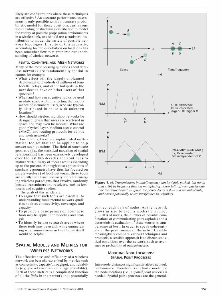
The challenge of spatial modeling can beillustrated by comparing the spatial resource totime/frequency resources. Wireless transmissionsneed to be separated in time, frequency, and/orspace to avoid excessive interference. Space is byfar the most challenging resource to use effi-ciently, for two reasons:• In space, transmitters and receivers are not

collocated• Power from undesired transmitters leaks in

space over relatively large distancesIn contrast, when using time or frequency divi-sion, transmitters and receivers are collocated(in time/frequency), and the spilling can be mini-mized. This is illustrated in Fig. 1. In time, whenturning off a transmitter, radiated power is driv-en to zero almost immediately. In frequency,waveforms are designed such that the power falloff is 100 dB or more per decade. In contrast,the falloff in space is only about 20–40dB/decade. For example, Wi-Fi devices arerequired to suppress their transmissions in fre-quency by 20 dB over just 2 MHz, which is only10 percent of their bandwidth and 0.01 percentof a decade (which would run to 24 GHz). Inshort, interference in time and frequency can beengineered, whereas interference in space is heldhostage by Maxwell’s equations and there arevery few practical options available to reduceinterference to neighboring receivers short ofreducing the transmit power; which would equal-ly affect the strength of the desired signal andthus not increase the signal-to-interference ratio.

RANDOM SPATIAL MODELSBecause spatial configurations may vary widelyover an enormous (often infinite) number ofpossibilities, one cannot design most systems foreach specific configuration but must instead con-sider a statistical spatial model for the node loca-tions. The usefulness of recent innovations suchas wireless network coding and interferencealignment depends critically on the relative posi-tions of transmitters and receivers: but just how

ABSTRACT

The performance of wireless networksdepends critically on their spatial configuration,because received signal power and interferencedepend critically on the distances betweennumerous transmitters and receivers. This is par-ticularly true in emerging network paradigmsthat may include femtocells, hotspots, relays,white space harvesters, and meshing approaches,which are often overlaid with traditional cellularnetworks. These heterogeneous approaches toproviding high-capacity network access are char-acterized by randomly located nodes, irregularlydeployed infrastructure, and uncertain spatialconfigurations due to factors like mobility andunplanned user-installed access points. Thismajor shift is just beginning, and it requires newdesign approaches that are robust to spatial ran-domness, just as wireless links have long beendesigned to be robust to fading. The objective ofthis article is to illustrate the power of spatialmodels and analytical techniques in the design ofwireless networks, and to provide an entry-leveltutorial.

NEW R&D TOOLS FOR WIRELESS COMMUNICATIONS

Jeffrey G. Andrews and Radha Krishna Ganti, The University of Texas at Austin

Martin Haenggi, University of Notre Dame

Nihar Jindal, University of Minnesota

Steven Weber, Drexel University

A Primer on Spatial Modeling andAnalysis in Wireless Networks

ANDREWS LAYOUT 10/20/10 3:31 PM Page 156

IEEE Communications Magazine • November 2010 157

likely are configurations where these techniquesare effective? An accurate performance assess-ment is only possible with an accurate proba-bilistic model for those positions. Just as oneuses a fading or shadowing distribution to modelthe variety of possible propagation environmentsin a wireless link, one should use a statistical dis-tribution to model the variety of possible net-work topologies. In spite of this necessity,accounting for the distribution on locations hasbeen somewhat slow to migrate into our under-standing of wireless networks.

FEMTO, COGNITIVE, AND MESH NETWORKSMany of the most pressing questions about wire-less networks are fundamentally spatial innature, for example:• What effect will the largely unplanned

deployment of hundreds of millions of fem-tocells, relays, and other hotspots in thenext decade have on other users of thatspectrum?

• When and how can cognitive radios be usedin white space without affecting the perfor-mance of incumbent users, who are typical-ly distributed in space with unknownlocations?

• How should wireless multihop networks bedesigned, given that users are scattered inspace and may even be mobile? What aregood physical layer, medium access control(MAC), and routing protocols for ad hocand mesh networks?Fortunately, there is a sophisticated mathe-

matical toolset that can be applied to helpanswer such questions. The field of stochasticgeometry (i.e., the statistical modeling of spatialrelationships) has been extensively developedover the last two decades and continues tomature with a flurry of recent results extendingup to the present. Although most applications ofstochastic geometry have thus far focused onpurely wireless (ad hoc) networks, these toolsare equally useful and necessary for other emerg-ing wireless paradigms that involve randomlylocated transmitters and receivers, such as fem-tocells and cognitive radios.

The goals of this article are:• To argue that such tools are essential to

understanding fundamental network quali-ties such as connectivity, coverage, andcapacity

• To provide a basic primer on how thesetools may be applied for modeling and anal-ysis

• To identify future research areas wherethese tools may be useful, while enumerat-ing what innovations in the theory itselfwould be helpful.

SPATIAL MODELS AND METRICS FORWIRELESS NETWORKS

The effectiveness and efficiency of a wirelessnetwork are best characterized by metrics suchas connectivity, capacity/throughput, and reliabil-ity (e.g., packet error rate or outage probability).Each of these metrics is a complicated functionof all the links in the network that potentially

connect each pair of nodes. As the networkgrows in size to even a moderate number(10–100) of nodes, the number of possible com-binations of communicating pairs explodes and adeterministic evaluation of these metrics is cum-bersome at best. In order to speak coherentlyabout the performance of the network and tomeaningfully compare various techniques andprotocols, a sensible approach is to discuss statis-tical conditions over the network, such as aver-ages or probability of outage/success.

MODELING NODE LOCATIONS:SPATIAL POINT PROCESSES

Inter-node distances significantly affect networkperformance. Therefore, a stochastic model forthe node locations (i.e., a spatial point process) isneeded. Spatial point processes are the general-

Figure 1. a): Transmissions in time/frequency can be tightly packed, but not inspace. (b) In frequency division multiplexing, power falls off very quickly out-side the desired band. In space, the power decay is slow and uncontrollable,and causes potentially severe interference to neighbors.

Space Time/frequency

(a)

(b)

A

y

x t,f

A

B

B

C

C

D

D

P

FDM

AB↓ ↓

f

>100dB/decadeTx, Rx colocatedlarger P higher R

CD

P

SDM

X

20-40dB/decade (dist.)Tx, Rx separatedSIR independent of P

A → B C → D

ANDREWS LAYOUT 10/20/10 3:31 PM Page 157

IEEE Communications Magazine • November 2010158

ization of point processes indexed by time tohigher dimensions, such as 2-D and 3-D space.Stochastic geometry provides the tools to ana-lyze important quantities such as interferencedistributions and link outages, and thus permitsstatistical statements about network performance[2, 3]. It also allows the designer to focus on asingle receiver or link by making the notion of atypical node or a typical link mathematically pre-cise. Due to its analytical tractability and practi-cal appeal in situations where transmitters and/orreceivers are located or move around randomlyover a large area, the (homogeneous) Poissonpoint process (PPP) has been by far the mostpopular spatial model. For example, in the 2-DPPP, each node takes up an independent loca-tion characterized by a pair of coordinates (xi,yi), the density of nodes in a unit area is λ, andso the average number of nodes in an area A isλA. Finally, the probability that there are nnodes in A is given by the Poisson distributionand thus equal to (λA)n e–λA/n!

Recent work has also considered more gener-al models such as cluster models — in whichnodes tend to cluster in certain locations — orhard-core models, in which nodes have a guaran-teed minimum separation, for example due to acarrier sensing MAC protocol that avoids nearbysimultaneous transmissions [2]. More generalpoint processes typically result in less tractableexpressions that include integrals that must benumerically evaluated, which is still much sim-pler than an exhaustive network simulation.Some useful point processes for wireless networkmodeling are summarized in Table 1, and a fewsample illustrations are given in Fig. 2.

SINR — THE BUILDING BLOCK METRICEach of the key metrics follows directly from thereceived signal-to-interference-plus-noise ratio(SINR) on one or more links, so understandingthe SINR is essential. The SINR is the instanta-neous ratio of desired energy to interference andnoise energy, and so is a random variable thatdepends on many factors. The most importantfactors are as follows.

The Distance between the Desired Trans-mitter and the Desired Receiver — Based onelectromagnetic laws, the desired received powerfalls off with distance and obeys an inversepower-law where the exponent is known as thepath loss exponent. In free space the power decayis quadratic with distance, but over ground thepath loss exponent is usually better modeled bya value between 2.5 and 4 because of scatteringand absorption. The difference in received powerbetween a 5 meter link and a 100 meter link is afactor of at least 400 (path loss exponent of 2),but is more likely 10,000 or more for more typi-cal path loss exponents. This multiple order-of-magnitude attenuation and dynamic range isfundamental to the behavior of wireless net-works.

The Set of Active Transmitters — There aremany potential combinations of active transmit-ters in even a moderate sized wireless network.The set of active transmitters is often chosen bythe MAC protocol. To each receiver, the otheractive transmitters appear to be interferers.1

The Sum Interference Power — The suminterference power depends on the set of inter-fering transmitters and their distances from eachdesired receiver. In networks of moderate tohigh density the interference power is usuallymuch larger than the noise power.

The Noise Power — The impact of the ambi-ent noise power on the SINR depends uponreceived signal and interference powers: underlow transmission power the SINR is noise-limit-ed, while under high transmission power theSINR is interference-limited.

Many other factors can affect the SINRincluding random propagation effects (fadingand shadowing), specific transceiver design prac-tices (for example, the use of multiple antennasor interference cancellation), and power control.But the spatial interactions are the most funda-mental and inescapable — general fading, shad-owing, and power control models can be (and

Table 1. Common spatial models, in approximate order of simplicity/tractability.

Point Process Key Properties Practical Example Reference

Poisson (PPP) Mutual independence between (transmitting)node locations.

Ad hoc networks with pure random channelaccess.

Fig. 3. Mostprior work.

Binomial Similar to PPP as far as i.i.d. node locations, butwith a fixed number of nodes in a given area.

A known number of relays or mobile usersdeployed at random in a cell of known size [4]

Poisson cluster(PCP)

Clustering of nodes, with independence betweencluster locations.

Sensor networks, military platoons, an urbannetwork with dense hotspots. [5]

Poisson plusPoisson Cluster

Independence between the PCP and the PPP.Attraction between nodes.

PPP represents the mobile users in a macrocelland the PCP represents femtocells or hotspots. Fig. 5. [6]

Matern hardcore Minimum distance between nodes. Carrier sensing wireless networks with colli-

sion avoidance, e.g. WiFi. Fig. 3. [2]

Determinantal Repulsion between nodes, e.g. Ginibre Process. CSMA networks, networks with soft minimumdistance. Fig. 2

1 Using two or more sepa-rate frequency bands addsa degree of freedom forscheduling and wouldusually reduce the numberof interferers per band, butin its essence the problemis unchanged in eachband. Hence we restrictour attention in this arti-cle to operation in a singleband.

ANDREWS LAYOUT 10/20/10 3:31 PM Page 158

IEEE Communications Magazine • November 2010 159

have been) added to the baseline model that isthe focus of this article. A fairly general but sim-ple mathematical description of the SINR at atypical node located at origin o is:

where hio is the (power) fading coefficient of thechannel to the desired receiver o from node i, ρi.is the transmit power of transmitter i, No is thenoise power, and Φ is the set of interfering nodes(Φ is a subset of all possible transmitters). Thedesired transmitter is a distance r from the desiredreceiver, while the ith interferer is a distance Xiaway. By drawing the distances according to aprobabilistic spatial model, the randomness inlocations along with many other basic aspects ofthe network (e.g., path loss) are consolidated intoa single random variable, the SINR.

We now will briefly overview how the SINRmay be used to specify and ultimately computemetrics of interest, namely the connectivity/cov-erage and the capacity/throughput. As shownbelow, it is possible (in fact preferable) to incor-porate reliability into both of these classes ofmetric, so considering reliability separately isunnecessary.

CONNECTIVITY AND COVERAGEThe connectivity of a random network can bedescribed as the probability that an arbitrary pairof nodes are able to exchange information at aspecified rate. For example, if this probability is0.9 for a random selection of a source-destina-tion pair, then one would say that the network is90 percent connected. The minimum powerrequirement for wireless network connectivity isintimately connected with percolation thresh-olds; this formed the basis for many early results.In the simplest case of direct transmission, i.e.,single hop communication, the probability ofconnectivity is simply Pr[SINR > β], where β isthe minimum required SINR that is consideredacceptable, and is a tunable parameter andSINR is the signal-to-interference and noiseratio of a typical link. Note that for a desiredrate R in bits per second, β ≈ Γ(2R – 1), where Γ≥ 1 is the SNR gap from Shannon rate signaling.

In many wireless networks of interest, a singlehop is all that is required or in fact allowed (e.g.,traditional cellular networks). In such cases, theregion of connectivity around a given transmitteris known as its coverage area. More generally, asource and a destination may communicate usingone or more intermediate relays, in which case apath through the network must be found whereeach hop has an SINR greater than β. Also, thecase where there is only one active flow in thenetwork (in which case there is no interferencefrom nodes not participating in transmitting thisflow) and the case where there are many flows,where each node may be serving as a relay forone or more flows, need to be distinguished.There are many ways to describe and quantifynetwork connectivity, but at the core, they allrequire that individual pairs are able to commu-nicate, which is dictated by the SINR.

THROUGHPUT

Throughput is one of the most important perfor-mance metrics for wireless networks, and a num-ber of different notions of throughput exist.

Link Throughput — Spatial models lend them-selves to an analytical characterization of the per-link throughput, which is a critical determinant ofend-to-end rate in multi-hop networks and is thequantity of interest for single-hop networks. Per-link throughput is dictated by the SINR, and canbe defined in different ways. The average per-link throughput is Ravg = E [log(1 + SINRij/Γ)],where the average is with respect to the sourcesof randomness encapsulated in the random vari-able SINR (e.g., locations and fading). This met-ric can be appropriate for settings in which thetransmitted rate is adjusted to the instantaneousSINR, whereas outage-based metrics are moreappropriate when dynamic rate adjustment is notperformed. The outage capacity of a link is thelargest rate (or mutual information) that can besupported with a certain probability, for example0.95, and so naturally includes reliability. Interms of SINR, this can be expressed in terms ofa target outage probability ε as

Cout = max log(1 + β) : Pr[SINR > β] > 1 – ε

For the network as a whole, it is then neces-sary to determine the outage Pr[SINR < β].However, this depends on the Tx-Rx distance,and the locations of the active transmitters.Clearly, if fewer transmitters are active, then theSINR and hence the outage capacity can beincreased, but the overall network throughputwould also decrease. It is necessary to balancethese two effects with a different metric. Onesuch metric is the transmission capacity, firstdefined in [7] as

τε = (1 – ε)λb

where λ is the maximum average number ofactive transmitters sending a rate of b b/s/Hzper unit area for which the outage probability isless than ε. In order words, the transmissioncapacity is the average number of successfulactive links of a certain rate that can be sup-ported per square meter in the network [8]. It

SINRh r

N h Xo

oo o

o i i io i

=+

−

∈−∑

ρ

ρ

α

αΦ

,

Figure 2. Three sample point processes. Poisson-distributed nodes have inde-pendent locations, whereas a Ginibre determinantal process can be used tomodel more evenly distributed nodes, and cluster process can be used tomodel situations where nodes are likely to be close to one another, e.g. due toterrain.

Cluster (Cox) processAttractive

4020-20

-40

-20

20

40

-40

Poisson processNeutral

4020-20

-40

-20

20

40

-40

Ginibre processRepulsive

4020-20

-40

-20

20

40

-40

ANDREWS LAYOUT 10/20/10 3:31 PM Page 159

IEEE Communications Magazine • November 2010160

has units of area spectral efficiency, for exam-ple b/s/Hz/m2. As will be shown below, thismetric is in fact computable over a wide rangeof network models.

End-to-End Rate — For large wireless net-works (e.g., ad hoc) where single hop communi-cation is not possible, it is desirable to know theend-to-end rate that is supportable between atypical source-destination pair in the network.This is much more difficult to compute becauseit depends on routing strategies, the retransmis-sion strategies, and further depends on the relia-bility and rate of each hop. For certain strategies,however, end-to-end rate is a simple function ofthe per-link throughput and thus can be comput-ed. Note also that end-to-end rate ties directly tothe transport capacity, which is an end-to-endrate metric of units bit-meters/sec that incorpo-rates distance and node locations, and givescredit in proportion to the distance the informa-tion is transported [9]. Measuring performancein terms of both achieved rate and distance trav-eled is also found in the effective forwardprogress metric used in early work in packetradio networks from the late 1970’s. Becausespatial models provide an explicit distribution ondistances, such models are also amenable toquantification of transport capacity.

APPLYING SPATIAL MODELSWe now consider three types of wireless net-works where spatial models play a central role:ad hoc networks, femtocells, and cognitive radio.

AD HOC NETWORKSAd hoc networks — purely wireless networks inwhich all nodes in the network must exchangeinformation with each other without any wiredbackhaul — are the framework in which spatialmodels have been most widely embraced.Indeed, the classical results on throughput scal-ing for ad hoc networks are fundamentally basedon a spatial model and a spatial metric in whichprogress is measured in terms of rate times dis-

tance, as just discussed. Scaling laws do notreveal the effect of physical layer algorithms,channel access protocols, so now we considerhow spatial models provide mechanisms to deter-mine other fundamental properties of an ad hocnetwork.

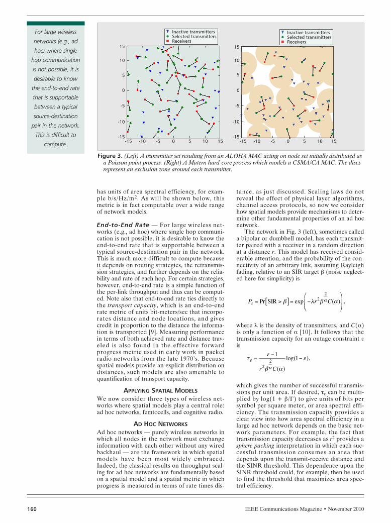
The network in Fig. 3 (left), sometimes calleda bipolar or dumbbell model, has each transmit-ter paired with a receiver in a random directionat a distance r. This model has received consid-erable attention, and the probability of the con-nectivity of an arbitrary link, assuming Rayleighfading, relative to an SIR target β (noise neglect-ed here for simplicity) is

where λ is the density of transmitters, and C(α)is only a function of α [10]. It follows that thetransmission capacity for an outage constraint εis

which gives the number of successful transmis-sions per unit area. If desired, τε can be multi-plied by log(1 + β/Γ) to give units of bits persymbol per square meter, or area spectral effi-ciency. The transmission capacity provides aclear view into how area spectral efficiency in alarge ad hoc network depends on the basic net-work parameters. For example, the fact thattransmission capacity decreases as r2 provides asphere packing interpretation in which each suc-cessful transmission consumes an area thatdepends upon the transmit-receive distance andthe SINR threshold. This dependence upon theSINR threshold could, for example, then be usedto find the threshold that maximizes area spec-tral efficiency.

τε

β α

εε

α

=−

−1

12

2

r C( )

log( ),

P r Cs = >[ ] = −⎛

⎝⎜⎜

⎞

⎠⎟⎟

Pr exp ( ) ,SIR β λ β αα22

Figure 3. (Left) A transmitter set resulting from an ALOHA MAC acting on node set initially distributed asa Poisson point process. (Right) A Matern hard-core process which models a CSMA/CA MAC. The discsrepresent an exclusion zone around each transmitter.

-10-15

-10

-15

-5

0

5

10

15

-5 0 5 10 15

Inactive transmittersSelected transmittersReceivers

-10 -15

-10

-15

-5

0

5

10

15

-5 0 5 10 15

Inactive transmitters Selected transmitters Receivers

For large wireless

networks (e.g., ad

hoc) where single

hop communication

is not possible, it is

desirable to know

the end-to-end rate

that is supportable

between a typical

source-destination

pair in the network.

This is difficult to

compute.

ANDREWS LAYOUT 10/20/10 3:31 PM Page 160

IEEE Communications Magazine • November 2010 161

The above result holds under the assumptionthat the set of active transmitters form a homo-geneous PPP (the receivers are thus not a partof the underlying process). However, as notedearlier, more sophisticated spatial models canalso be analyzed, such as assuming the activetransmitters are distributed according to a hard-core process (emulating a CSMA/CA MAC) orthat the transmitters and receivers are chosenfrom a common point process. More sophisti-cated transmission protocols can also be intro-duced fairly easily in the model by simplychanging the starting SINR expression given inEq. 1. For example, multi-antenna beamform-ing, spread spectrum, and power control can allbe handled through appropriate modification ofthe SINR. An overview of these and other gen-eralizations is given in [8]. This model has alsobeen extended recently to a basic multihopmodel in [11].

COGNITIVE RADIOS AND WHITE SPACEScarcity of bandwidth and the allegedly sparseuse of licensed spectrum by incumbents has ledto the popularity of cognitive radios, whichattempt to find locally unused spectrum andcommunicate over it opportunistically. The via-bility of this aggressive new approach to fre-quency reuse has been endorsed by the UnitedStates FCC in its 2009 Whitespace ruling, whichlays down conditions under which cognitiveradios can utilize previously licensed spectrum,namely the former analog TV bands, the majori-ty of which are in the 470–806 MHz range. Aprimary consideration of a cognitive radio is thelikelihood of interfering with a primary, orlicensed, user of the spectrum. The probabilityof this occurring must be held small, and it clear-ly depends on the spatial density and the typical-ly unknown locations of the primary receivers.

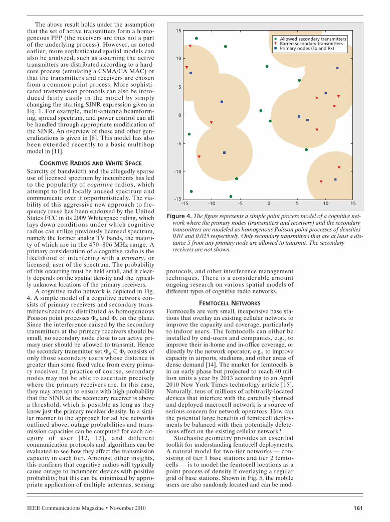
A cognitive radio network is depicted in Fig.4. A simple model of a cognitive network con-sists of primary receivers and secondary trans-mitters/receivers distributed as homogeneousPoisson point processes Φp and Φs on the plane.Since the interference caused by the secondarytransmitters at the primary receivers should besmall, no secondary node close to an active pri-mary user should be allowed to transmit. Hencethe secondary transmitter set Φst ⊂ Φs consists ofonly those secondary users whose distance isgreater than some fixed value from every prima-ry receiver. In practice of course, secondarynodes may not be able to ascertain preciselywhere the primary receivers are. In this case,they may attempt to ensure with high probabilitythat the SINR at the secondary receiver is abovea threshold, which is possible as long as theyknow just the primary receiver density. In a simi-lar manner to the approach for ad hoc networksoutlined above, outage probabilities and trans-mission capacities can be computed for each cat-egory of user [12, 13], and differentcommunication protocols and algorithms can beevaluated to see how they affect the transmissioncapacity in each tier. Amongst other insights,this confirms that cognitive radios will typicallycause outage to incumbent devices with positiveprobability; but this can be minimized by appro-priate application of multiple antennas, sensing

protocols, and other interference managementtechniques. There is a considerable amountongoing research on various spatial models ofdifferent types of cognitive radio networks.

FEMTOCELL NETWORKSFemtocells are very small, inexpensive base sta-tions that overlay an existing cellular network toimprove the capacity and coverage, particularlyto indoor users. The femtocells can either beinstalled by end-users and companies, e.g., toimprove their in-home and in-office coverage, ordirectly by the network operator, e.g., to improvecapacity in airports, stadiums, and other areas ofdense demand [14]. The market for femtocells isin an early phase but projected to reach 40 mil-lion units a year by 2013 according to an April2010 New York Times technology article [15].Naturally, tens of millions of arbitrarily-locateddevices that interfere with the carefully plannedand deployed macrocell network is a source ofserious concern for network operators. How canthe potential large benefits of femtocell deploy-ments be balanced with their potentially delete-rious effect on the existing cellular network?

Stochastic geometry provides an essentialtoolkit for understanding femtocell deployments.A natural model for two-tier networks — con-sisting of tier 1 base stations and tier 2 femto-cells — is to model the femtocell locations as apoint process of density lf overlaying a regulargrid of base stations. Shown in Fig. 5, the mobileusers are also randomly located and can be mod-

Figure 4. The figure represents a simple point process model of a cognitive net-work where the primary nodes (transmitters and receivers) and the secondarytransmitters are modeled as homogenous Poisson point processes of densities0.01 and 0.025 respectively. Only secondary transmitters that are at least a dis-tance 5 from any primary node are allowed to transmit. The secondaryreceivers are not shown.

-10 -15

-10

-15

-5

0

5

10

15

-5 0 5 10 15

Allowed secondary transmitters Barred secondary transmitters Primary nodes (Tx and Rx)

ANDREWS LAYOUT 10/20/10 3:31 PM Page 161

IEEE Communications Magazine • November 2010162

eled as a point process of density lc, where typi-cally lc >> lf. The interference at a given mobileuser, for example, now consists of interferencefrom neighboring base stations as well as fromrandomly placed femtocell base stations. Similar-ly, the interference at a femtocell base station isthe aggregation of interference from all theuplink mobile users, and is typically dominatedby a small number of mobile users transmittingat relatively high power up to the main base sta-tion. Again, each receiver’s SINR can be careful-ly modeled using random spatial models for theinterference from femtocells, mobile users, basestations, and femtocell users, as appropriate. Theallowable density of mobile users can then betraded off with the femtocell density using out-age probability or transmission capacity, and dif-ferent techniques for cross-tier interferencesuppression and avoidance can be evaluated [6].This is conceptually similar to a capacity region,where now the two competing axes are femtocellvs. macrocell achievable rate.

FUTURE DIRECTIONS FORSPATIAL MODELS

Random spatial models will become increasinglyrelevant for the dense and complex wireless net-works that will emerge over the next decade.This article has attempted to give a high-levelview of the importance of such models and howthey can be applied to different types of wireless

networks. Much more work is needed, on thefundamental mathematics, confirmation of theaccuracy of the models in the various scenarios,and further application of spatial models toemerging candidate protocols and networks.

The most tractable results from stochasticgeometry tend to rely on a few assumptions thatmay not accurately hold in practice. The mostimportant are the homogeneous Poisson pointprocess for transmitting node locations and theneglect of temporal and spatial correlations. It isdesirable to relax these assumptions in the com-ing years. There will be an ongoing trade-offbetween tractability and generality, but as ran-dom spatial models gain acceptance, it may bepossible to improve the perceived tractability byidentifying canonical solutions that may not beclosed-form. For example, most probability oferror expressions include an integral over Gaus-sian tail, accepted universally as the Q-function.The Q-function is not closed-form, but is oftentreated as such because it is so common. Similar-ly for complex spatial models, it may be neces-sary to simply define and name often-recurringintegrals and live with them.

Even when analysis with random spatial mod-els is not fully tractable, network performancecan often be easily simulated because network-wide performance can be characterized by theperformance of a typical node. Thus, agreedupon random spatial models will allow for stan-dardized rapid benchmarking of wireless net-work protocols, just as well-accepted AWGNand fading channel models have been indispens-able for fairly comparing techniques for point-to-point links.

ACKNOWLEDGMENTSThe authors gratefully acknowledge feedbackand suggestions from Angel Lozano, RobertHeath, Illsoo Sohn, Kostas Stamatiou, JunZhang, and the anonymous reviewers.

REFERENCES[1] D. C. Cox and H. Lee, “Physical Relationships: Exploring

Fundamental Relationships Between Transmission Rateand Range for Wireless Systems,” IEEE MicrowaveMag., Aug. 2008, pp. 89–94.

[2] F. Baccelli and B. Blaszczyszyn, Stochastic Geometry andWireless Networks, Foundations and Trends in Net-working, NOW Publishers.

[3] M. Haenggi and R. K. Ganti, “Interference in LargeWireless Networks,” Foundations & Trends Net., 2009.

[4] J. Zhang and J. G. Andrews, “Distributed Antenna Sys-tems with Randomness,” IEEE Trans. Wireless Com-mun., Sept. 2008.

[5] R. K. Ganti and M. Haenggi, “Interference and Outagein Clustered Wireless Ad Hoc Networks,” IEEE Trans.Info. Theory, Sept. 2009.

[6] V. Chandrasekhar and J. G. Andrews, “Uplink Capacityand Interference Avoidance for Two-Tier Femtocell Net-works,” IEEE Trans. Wireless Commun., July 2009.

[7] S. Weber et al., “Transmission Capacity of Wireless AdHoc Networks with Outage Constraints,” IEEE Trans.Info. Theory, Dec. 2005.

[8] S. Weber, J. G. Andrews, and N. Jindal, “An OverviewOf The Transmission Capacity Of Wireless Networks,”IEEE Trans. Commun., to be published.

[9] P. Gupta and P. R. Kumar, “The Capacity of WirelessNetworks,” IEEE Trans. Info. Theory, Mar. 2000.

[10] F. Baccelli, B. Blaszczyszyn, and P. Mühlethaler, “AnALOHA Protocol for Multihop Mobile Wireless Net-works,” IEEE Trans. Info. Theory, Feb. 2006.

[11] J. G. Andrews et al., “Random Access TransportCapacity,” IEEE Trans. Wireless Commun., June 2010.

Figure 5. A square cell overlaid by femtocells. The femto BS's are modeled by aPoisson point process (blue squares) and they serve a disc of radius 2. Thegreen dots represent mobile users (non-femto cell users) which communicatewith the main base station, which is represented as a black diamond. Notethat it is possible for mobile users to be inside the range of a femtocell but notuse the femtocell.

Base station Mobile users Femtocell BS Femto users

-10 -15

-10

-15

-5

0

5

10

15

-5 0 5 10 15

ANDREWS LAYOUT 10/20/10 3:31 PM Page 162

IEEE Communications Magazine • November 2010 163

[12] C. Yin et al., “Transmission Capacities for OverlaidWireless Ad Hoc Networks with Outage Constraints,”IEEE ICC, Dresden, Germany, June 2009.

[13] K. Huang, V. Lau, and Y. Chen, “Spectrum Sharingbetween Cellular and Mobile Ad Hoc Networks: Trans-mission Capacity Trade-Off,” IEEE JSAC, Sept. 2009, pp.1256–67.

[14] V. Chandrasekhar, J. G. Andrews, and A. Gatherer,“Femtocell Networks: a Survey,” IEEE Commun. Mag.,Sept. 2008.

[15] M. Richtel, “Bringing You a Signal You’re Already Pay-ing For,” The New York Times, Apr. 6, 2010.

ADDITIONAL READING[1] M. Haenggi et al., “Stochastic Geometry and Random

Graphs for the Analysis and Design of Wireless Net-works,” IEEE JSAC, Sept. 2009.

[2] D. Stoyan, W. Kendall, and J. Mecke, Stochastic Geome-try and its Applications, 2nd Ed., Wiley, 1996.

[3] S. Weber, J. G. Andrews, and N. Jindal, “The Effect ofFading, Channel Inversion, and Threshold Schedulingon Ad Hoc Networks,” IEEE Trans. Info. Theory, Nov.2007.

[4] J. F. C. Kingman, Poisson Processes, Oxford UniversityPress, 1993.

[5] M. Z. Win, P. C. Pinto, and L. A. Shepp, “A Mathemati-cal Theory of Network Interference and Its Applica-tions,” Proc. IEEE, Feb. 2009.

BIOGRAPHIESJEFFREY G. ANDREWS [SM‘06] (jandrews@ece.utexas.edu) isan Associate Professor in the ECE Department at UT Austin,where he is the Director of the Wireless Networking andCommunications Group. He received a B.S. with High Dis-tinction from Harvey Mudd College and his M.S. and Ph.D.from Stanford University. He has previously worked atQualcomm and consulted for the WiMAX Forum, Microsoft,ADC, Apple, Clearwire, and NASA. He is co-author of Fun-damentals of WiMAX (Prentice-Hall, 2007) and Fundamen-tals of LTE (Prentice-Hall, 2010). He received the NSFCAREER award in 2007 and is the Principal Investigator ofa nine university team in DARPA’s Information Theory forMobile Ad Hoc Networks program. He has received bestpaper awards at IEEE GLOBECOM (2006 and 2009) andAsilomar (2008), the latter two for applications of stochas-tic geometry to femtocells, and the 2010 IEEE Communica-tions Society Best Tutorial Paper award for “StochasticGeometry and Random Graphs for the Analysis and Designof Wireless Networks.”

RADHA KRISHNA GANTI [M’10] is a Postdoctoral researcher inthe Wireless Networking and Communications Group at UTAustin. He received his B.Tech. and M.Tech. in EE fromIndian Institute of Technology, Madras, and Masters inApplied Math and Ph.D. in EE from University of NotreDame in 2009. His doctoral work focused on the spatialanalysis of interference networks using tools from stochas-tic geometry. He is co-author of the monograph Interfer-ence in Large Wireless Networks.

MARTIN HAENGGI [SM‘04] is an Associate Professor in the EEDepartment at the University of Notre Dame. He receivedthe M.S. and Ph.D. degrees from the Swiss Federal Insti-tute of Technology in Zurich, Switzerland (ETHZ) in 1995and 1999, respectively. He received the ETH Medal forboth his M.Sc. and Ph.D. theses and a CAREER award fromthe U.S. National Science Foundation in 2005. He servedas the Lead Guest Editor for an issue of the IEEE Journalon Selected Areas in Communications on stochastic geom-etry and random graphs for wireless networks in 2009and currently is an Associate Editor of the IEEE Transac-tions on Mobile Computing and the ACM Transactions onSensor Networks. He co-authored the monograph Interfer-ence in Large Wireless Networks (NOW Publishers, 2009),and received the 2010 IEEE Communications Society BestTutorial Paper award for “Stochastic Geometry and Ran-dom Graphs for the Analysis and Design of Wireless Net-works”.

NIHAR JINDAL [M‘04] is an assistant professor in the ECEDepartment at the University of Minnesota. He received hisB.S. from U.C. Berkeley, and his M.S. and Ph.D. from Stan-ford University. He is currently an Associate Editor for theIEEE Transactions on Communications, and has also servedas a guest editor for the EURASIP Journal on Wireless Com-munications Networking. He received the NSF CAREERaward in 2007 and the University of Minnesota GuillermoE. Borja Award in 2010. He also received the IEEE Commu-nications Society and Information Theory Society JointPaper Award in 2005, and the Best Paper Award for theIEEE Journal on Selected Areas in Communications (IEEELeonard G. Abraham Prize) in 2009.

STEVEN WEBER [M‘03] is an Associate Professor in the ECEDepartment at Drexel University. He received the B.S. fromMarquette University in 1996, and the M.S. and Ph.D. fromThe University of Texas at Austin in 1999 and 2003 respec-tively. His research interests are centered around mathe-matical modeling of computer and communicationnetworks, specifically streaming multimedia and ad hocnetworks.

ANDREWS LAYOUT 10/20/10 3:31 PM Page 163