A PRICE RESPONSE MODEL DEVELOPEDFROM PERCEPTUAL THEORIES

Gurumurthy, K.University of Texas at Dallas

John D.C. LittleM.I.T. School of Management

Sloan School Working Paper # 3038-89June 1989

Marketing Center Working Paper 89-5

This is a revised version of a paper originally presented at the MarketingScience Conference in Dallas, March 1986, under the title "A Pricing Model Basedon Perception Theories and its Testing on Scanner Panel Data."

/II

ABSTRACT

Theories of perception and judgment suggest a structure for a price and promotionresponse model that is then calibrated on scanner panel data for coffee.Adaptation level and assimilation-contrast theory imply the existence of areference price and a possible region of customer insensitivity to price(latitude of price acceptance). Prospect theory suggests an asymmetric responseto price changes. Attribution theory would predict a negative effect ofpromotional frequency on product choice. These concepts are operationalized andimbedded in a multinomial logit model.

Two scanner panel databases for regular ground coffee (SAMI and IRI) provide anopportunity to test the model empirically. The results show an asymmetric priceresponse with customers more sensitive to price increases than decreases. Thisis as would be predicted by prospect theory. There is evidence of a region ofprice insensitivity and also for a negative effect of promotional frequency onpurchase probability. The results are consistent across the two independentdatabases.

III

INTRODUCTION

A hierarchy of useful knowledge for providing assistance to marketing managersmight be as follows:

(1) General constructs for thinking about marketing phenomena(e.g. price elasticity),

(2) Rough magnitudes of the effects (e.g. price elasticity is inthe range of 2 to 3 for brands in the coffee category),

(3) Measurements as close as possible to the case of practicalinterest to the decision maker (e.g. Butternut Coffee onepound size has a share-price elasticity of 2.3 in KansasCity).

In this paper we turn to the psychological literature for broad constructs thatmay be applicable to product pricing and promotion. As a potential contributionto (1), we relate several to the pricing of consumer package goods. For (2) wetry to construct models that will permit measurements that give ranges ofmagnitudes for certain price phenomena. Ultimately this may lead to (3), modelsfor specific products in specific practical situations.

Price response models involve a number of issues. One is whether actual priceor a perceptually-based transformation of price should be used in modeling thesales-price and share-price relationships. Most economists and many marketershave used actual price, either absolute or relative. By contrast,psychologists, some other marketers and an increasing number of economists havefocused on the perceptual aspects of price and, consequently, have put forwardsuch concepts as price-ending effects (Monroe 1973), price thresholds (Uhl andBrown 1971, Monroe 1971), price-quality relationships (Gabor and Granger 1966,Monroe 1973) and reference price (Emery 1970, Monroe 1973). A presumption inthese papers is that perceived price is what matters and that perceived priceitself is dependent on various factors such as current price, past price andother marketing stimuli. More recently, steps have been taken to meld the twoapproaches, especially in the study of reference price (Rinne 1981, Winer 1986,Raman and Bass 1988, Lattin and Bucklin 1987, Kalwani, Rinne, Sugita and Yim1988).

We start with the psychologist's view in the sense of looking to theories ofperception and judgment for constructs from which to develop pricing andpromotion response models, although we shall happily borrow from the economicliterature as applicable. Four potentially relevant psychological theories are:adaptation level, assimilation-contrast, prospect, and attribution. The firstthree will motivate a price response model in which each theory provides aconstruct for a particular aspect: adaptation level theory for reference price,assimilation-contrast theory for latitude of price acceptance and prospecttheory for asymmetric customer response. The fourth, attribution theory,motivates a model of the effect of promotional frequency on purchasing. Weoperationalize these concepts for our particular setting, estimate modelparameters from data sets, and compare the results with theoretical predictions.

1

Much of the empirical work on price has examined relationships at the aggregatelevel. However, aggregate data can obscure valuable information and behavioralprocesses that are taking place at the household level. The availability ofdata from scanner panels provides an opportunity for building and calibratingmodels based on individual decision-making units. Disaggregate models fit wellwith psychological theories since these ordinarily deal with the individual.

In building and testing our models we shall not be testing the pyschologicaltheories, since these have already been shown valid through extensiveexperimentation. We shall be examining whether phenomena suggested by thetheories can be found in our marketing data using the models we develop.

Two scanner panel data sets on coffee purchases, one from Selling AreasMarketing, Inc. (SAMI) and the other from Information Resources, Inc. (IRI)provide an empirical base for calibrating and testing the models.

THEORETICAL MOTIVATION

ADAPTATION LEVEL THEORY

We use adaptation level theory to motivate reference price and its change as acustomer encounters new information.

Adaptation level theory (Helson, 1964) states that the perceived magnitude andeffect of a stimulus at any given time depends on the relation of that stimulusto preceding stimuli. The prior stimuli create an adaptation level andsubsequent stimuli are judged in relation to it. The judgement and,consequently, the response to a stimulus depend on the relationship between thephysical value of that stimulus and the value of the current adaptation level.According to Helson (1964), a change in a stimulus causes "an initial rapidchange in activity and sensitivity .... followed by a constant level of activityif the stimulus is continued at a constant intensity."

The adaptation level is the stimulus value at which the scale of judgment iscentered or anchored. It is usually taken to be a weighted logarithmic mean ofthe various physical values of the stimuli. Each of the judgments is in turndetermined by the ratio of the stimulus to the adaptation level. Inpsychophysics research, the test stimuli often increase geometrically and thelogarithmic mean fits well. However, in our case, the changes of stimulus arerelatively small (from 0 to about 20%) and so we shall use linear models, whichare much simpler and are reasonably equivalent over the ranges being considered.This is because for small x, log(l+x) x.

According to the theory, the past and present context of experience defines anadaptation level, or reference point, relative to which new stimuli areperceived and compared. A simple illustration of this would be as follows. Ifa person repeatedly lifts a weight of 100 grams, he or she then becomesaccustomed to this weight, i.e., adapts to it, and the adaptation level becomes100 grams.

2

III

Application to ricing. For pricing, the theory suggests an adaptation levelthat depends on previous price experience. The adaptation level will be calledthe reference price. In most cases, this will not be a price that physicallyappears on any goods but a price that customers are assumed to form in theirminds as a result of experience.

Various operationalizations appear in the literature. Rinne (1981) comparesthree approaches: (1) setting reference price equal to previous price (2) takingreference price as the weighted mean of the logs of past observations assuggested by Helson (1964), and (3) using an exponential smoothing modelmotivated by Friedman's (1979) general theory of adaptive expectations. Rinnethe imbeds each reference price model in a share-price response equation whoseparameters are estimated from a dataset. He finds that models (2) and (3)provide superior fits compared to (1) but neither (2) nor (3) dominates theother.

Raman and Bass (1988) start from an adaptive expectations view of referenceprice but seek to incorporate the additional phenomenon of price thresholds(Monroe 1973). The basic idea is that consumers have a region of relative priceinsensitivity about reference price but that at some threshold on either sideprice response changes and becomes much more pronounced. Raman and Bass,working with aggregate data, determine reference price using a Box-Jenkins auto-regressive model on historical prices. The reference price expression is thenimbedded in a model of market share response to price and a switching regressionmethodology used to identify thresholds.

Winer (1986) tests two different reference price formulation, one based on anextrapolative expectations hypothesis and the other a rational expectationshypothesis. After estimating the parameters of each formulation on his dataset, he inserts the reference price into a model relating purchase probabilityto marketing maix variables. His results do not show a marked differencebetween the formulations.

Two recent papers build even richer models for the formation of reference price.In Lattin and Bucklin (1987) customers form a reference discount if they areexposed to in-store price-cuts to such a degree that they cross a prescribedthreshold level. Thereupon, they tend to expect a discount and so requirebigger discounts to achieve the same level of purchase probability that wouldhave occurred had they not crossed the threshold. Kalwani, Rinne, Sugita andYim (1988) have added other variables besides past prices to their model ofreference price. Such variables include promotional frequency and the pronenessof the household to buy on promotion.

We wish a relatively simple operationalization of reference price thatnevertheless captures the basic idea that a customer modifies his or her viewof price as new information is encountered. A parsimonious way to do this iswith an exponential smoothing process, and the literature cited suggests thatit should work well. In the terminology of several of the above papers, we areusing an adaptive expectations approach. For each household and product:

current reference price - (carry-over constant)x(previous reference price)+ (1 - carry-over constant)x(previous actual price).

3

III

Further details will be developed below.

PROSPECT THEORY

A number of marketing writers have suggested that customers may have differentresponses to price increases and decreases (Pessemier 1960, Uhl and Brown 1971,Monroe 1976, Rinne 1981, Raman and Bass 1988). Usually it is suggested thatcustomers respond more negatively to price increases than they do positively todecreases. The empirical work of Pessemier (1960), Uhl and Brown (1971) andRaman and Bass (1988) supports this view, although Monroe (1976) in laboratoryexperiments reports the opposite and Rinne's empirical results are mixed. Inany case it would be desirable to have a theory more general than pricing itselfto motivate a model of the phenomenon.

Prospect theory (Kahneman and Tversky 1979) is a candidate. It was developedas an alternative to classical expected utility theory for the purpose ofdescribing and predicting individual choice behavior under risk. As a resultof many experiments, the authors and others have shown, first of all, thatchoice often depends on the way a problem is posed as well as on thecharacteristics considered in classical theories. Prospect theory, therefore,introduces the concept of a 'frame' or 'reference' and outcomes are expressedas gains or losses from a reference point.

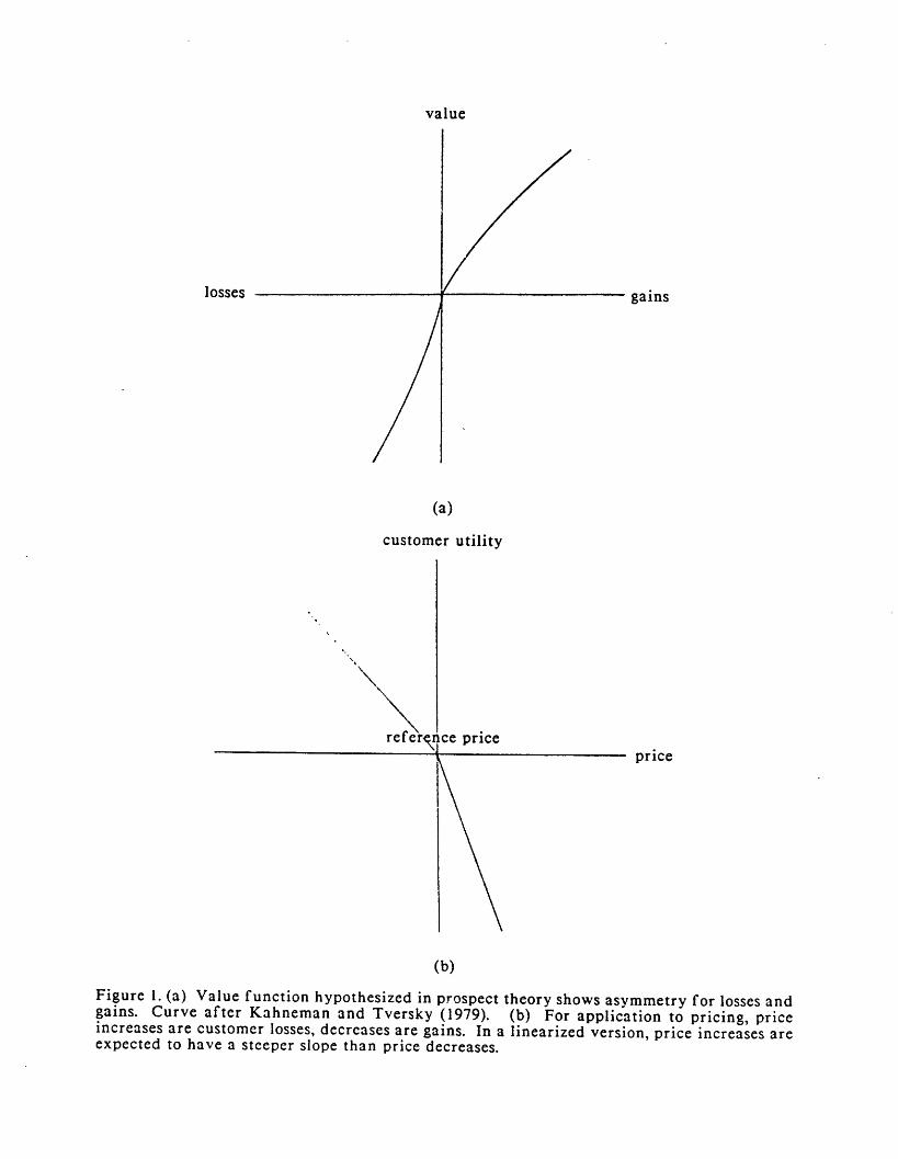
Secondly, the experiments reveal an asymmetric relationship between thesubjective values of the outcomes and objectively calculated expected values.The loss of a given amount is viewed more severely than the gain of the sameamount. The curve is also concave above the reference point and convex belowit. Figure 1, after Kahneman and Tversky (1979), sketches a value function withthese properties.

In marketing Thaler (1985) has used prospect theory to good advantage,supplementing it with constructs of his own, to explain a wide variety ofconsumer choice phenomena. Our use of prospect theory corresponds to hisconcept of transaction utility.

Application to pricing. For the case of pricing, an increase is a loss in valuefor the customer and a decrease a gain. The price response function suggestedby prospect theory is a reflection of Figure 1 across the vertical axis andtherefore appears as in Figure 2. Notice that we have taken the reference priceas the reference point for gains and losses and that we indicate a steeper slopefor price increases (losses) than price decreases (gains). We shall not attemptto look for the concavity-convexity property of the curve and so represent itwith two linear segments.

ASSIMILATION-CONTRAST THEORY

Assimilation-contrast theory suggests that, in the neighborhood of a referenceprice, customers are likely to perceive prices as different from actual values,tending to downplay small differences from the reference and exaggerating largeones. This leads to a concept of 'latitude of acceptance', a range of relative

4

value

losses gains

(a)

customer utility

price

(b)

Figure 1. (a) Value function hypothesized in prospect theory shows asymmetry for losses andgains. Curve after Kahneman and Tversky (1979). (b) For application to pricing, priceincreases are customer losses, decreases are gains. In a linearized version, price increases areexpected to have a steeper slope than price decreases.

price insensitivity. Related to this is the notion of a price threshold usedby Monroe (1979) and by Raman and Bass (1988).

A number of marketing writers have applied assimilation theory to priceperceptions (Emery 1970, Monroe 1971, 1973, Sawyer and Dickson 1984). However,two rather different ideas are discussed. Emery (1970) speaks of "an amount ofprice variation that has no effect on sales". Sawyer and Dickson (1984) drawa flat place on a curve of perceived price vs. actual price. Raman and Bass(1988) speak of a "region of indifference about a reference price such thatchanges in price within this region produce no change in perception." It s inthis sense that we use the term.

However, 'latitude of acceptance' is also used to refer to a broad range ofprices acceptable for a product class without implying indifference among theprices of individual items. Sherif (1963) uses the term this way in apioneering psychological study involving price perceptions, as does Monroe(1971) who also uses the term threshold to indicate the boundaries of thelatitude of price acceptance. The two uses of latitude of acceptance and pricethreshold are confusing but do not appear t be conflicting. Rather they aretwo different applications of the theory: one to different prices for the sameproduct and the other to prices of different products in the same category.

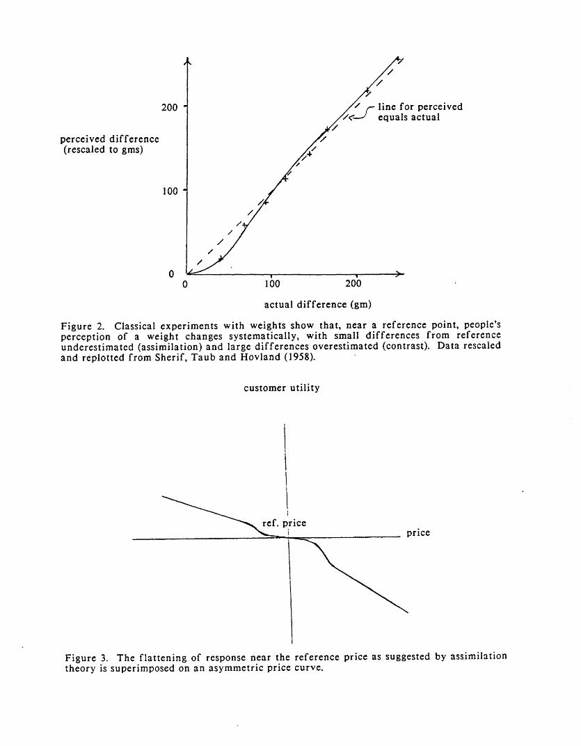
To stay close to the basic pyschophysical phenomenon as it might apply in ourcase, we describe the classical work of Sherif, Taub and Hovland (1958). Theauthors conducted experiments to determine the effect of an anchoring weight onpeople's judgments of a series of other weights. Subjects lifted an anchorweight several times and then judged each of the "series weights" on a 1 to 6scale. Each anchor was a different amount heavier than the range of the seriesweights. The authors found that, when the anchor weights were close to theseries, subjects assigned higher values to the series weights than when theanchor was absent. This is called the assimilation effect: the judgment isdrawn toward the anchor. On the other hand, as the anchor was moved far abovethe top value of the series, subjects assigned lower values to the seriesweights than when the anchor was absent. This is called the contrast effect:the judgment is driven away from the anchor. The same assimilation and contrastphenomena occurred for anchors lighter than the series.

The assimilation effect is particularly important, since it provides thetheoretical basis for a latitude of acceptance. Consequently we have rescaledand replotted the data of Sherif, Taub and Hovland so that it is in the form ofresponse to deviations from a fixed reference point (anchor). The resultsappear in Figure 2 with backup details in Appendix 1. Figure 2 clearly showsa depressed place under the 450 line representing assimilation near the origin,although lack of points makes it difficult to determine the exact shape. Thecontrast effect, which comes out vividly in the histograms of the originalarticle, is muted here by rescaling. Nevertheless, response is higher than the450 line for large deviations, as would be predicted by the contrast effect.After reflection across the horizontal axis, Figure 2 provides insight on howa price response curve might look for positive deviations from reference.

Application to pricing. As discussed, he assimilation effect suggests thatwithin a certain range about an anchor price, prices deviations may be perceived

6

III

200

perceived difference(rescaled to gms)

100

0

or perceiveds actual

0 100 200

actual difference (gm)

Figure 2. Classical experiments with weights show that, near a reference point, people'sperception of a weight changes systematically, with small differences from referenceunderestimated (assimilation) and large differences overestimated (contrast). Data rescaledand replotted from Sherif, Taub and Hovland (1958).

customer utility

price

Figure 3. The flattening of response near the reference price as suggested by assimilationtheory is superimposed on an asymmetric price curve.

I

I

III

as smaller than they actually are. Outside this range, or "latitude ofacceptance," the contrast effect implies that a person will not only takenotice of a price difference but may exaggerate it. In Figure 3 we sketch thisphenomenon superimposed on an asymmetric price response curve.

The width of a latitude of price acceptance will vary. When a customer hasbecome used to a single price for a long time, the latitude is likely to benarrow. An illustration might be a subway or bus fare which has been in effectfor several years. Any change, even a small one, is quickly noticed. However,when a person is unsure of the 'customary price' because price has variedconsiderably in the past, the latitude of acceptance is likely to be great. Acurrent example is airline fares; price wars and the proliferation of specialfares have introduced great price uncertainty so that a customer often hasdifficulty perceiving whether a quoted fare is high or low. With respect tofood products, Uhl and Brown (1971) found that customers' ability to perceiveprice changes was weaker for products with frequent price changes than forproducts with more stable prices.

Two issues now arise: First, how is the anchor point determined? Our approachis to take reference price as the anchor point. Second, what is an appropriatemeasure of latitude of price acceptance? Here we assume that latitude varieswith the situation and can be related to price variability in ways to beoperationalized below.

COMBINING THEORIES INTO A PRICING MODEL

A combined theory would have the following features. Each individual would havea reference price that depends on past price experience and so changes withtime. Around the reference price would be a latitude of price acceptance inwhich the customer is relatively insensitive to price changes. The width of thelatitude would depend on the price variation experienced by the customer and soadapts over time. Beyond the end points of the latitude of acceptance, pricesensitivity would take a sharp increase because of the contrast effect.Finally, outside the latitude of acceptance, the response to price decreases(gains) should be steeper than to price increases (losses).

These several ideas can be represented in a set of models of increasingcomplexity, each adding a new phenomenom, as shown in Figure 4. Figure 4a showsa simple linear response to deviations from reference price. Figure 4bintroduces asymmetry as expected from prospect theory. Figure 4c further addsa piece-wise linear, potentially flat segment to represent a latitude ofacceptance.

ATTRIBUTION THEORY

Attribution theory predicts that, although promotions may increase theprobability of immediate purchase, they may also create a negative after-effecton the customer's perceived value of a product. This idea was first introducedand supported empirically by Dodson, Tybout and Sternthal (1978).

8

Customer Utility

Figure 4 (a)

Customer Utility

. . , _ \_,

Customer Utility

Figure 4 (c)

Figure 4. A family of price response models of increasing complexity. (a) Customer utility isnegatively related to price in a simple linear fashion. (b) Prospect theory implies a steeperslope for price increases than decreases. (c) Assimilation theory suggests that small changesfrom reference will be underestimated.

Price

Price

Price

A central proposition of attribution theory is that individuals determine theirattitude toward an object in part by examining their own behavior and thecircumstances surrounding it. People tend to ascribe their behavior to eitherinternal or external causes. If an individual attributes her/his behavior toher/his own beliefs then the probability of repeating that behavior is enhanced.However, if there is a plausible external cause, then the behavior will oftenbe ascribed to that cause and the probability of repeating the behavior isdiminished.

Application to promotion. Attribution theory would predict that the higher thefrequency of promotion, the lower will be the probability of purchase in asubsequent period. The argument is follows: Suppose there is a brand A whichis promoted fairly frequently. Let us assume that a customer purchases brandA initially for its intrinsic value. However, since the brand is often onpromotion, the customer may start to feel that he/she is purchasing the brandbecause it is on promotion, i.e., the customer may begin to ascribe the causeof purchase to promotion (an external cause) rather than to his/her ownpreference (an internal cause). To the extent that the purchases are attributedto promotion, a diminishing in perceived evalue will take place. For furtherdiscussion, see Dodson, Tybout and Sternthal (1978).

One may note that the negative attribution is especially likely to occur if thebrand is promoted frequently. Therefore, a negative relation is expectedbetween the frequency of promotion and probability of purchase. Notice,however, that one would still expect a positive impact of promotion on thecurrent purchase relative to the probability of making that purchase without thepromotion.

A number of writers have noted that the recent purchase of a product onpromotion tends to lower the probability of purchasing it on the next occasion,other variables being held constant. See for example, Shoemaker and Shoaf(1977) and Guadagni and Little (1983). The approach here differs in that itchooses a broad measure, promotional frequency, to characterize the overallpromotional activity of the product.

The phenomenon is modeled by its own variable and so can be treated as aseparable submodel in our overall price response function.

THE MULTINOMIAL LOGIT MODEL OF CHOICE

The multinomial logit model of probability of choice is well suited for modelingat the household level and has been used successfully in a number of marketingstudies (Gensch and Recker 1979, Guadagni and Little 1983). In particular wedraw heavily on the last. Essentially, we remove the pricing part of Guadagniand Little's model and substitute a new, behaviorally motivated structure.Related modifications are also made to promotion variables.

The multinomial logit, as it will be used here, calculates the probability ofchoice by an individual as a function of inferred utilities for a set ofalternatives. Let

10

pik - probability that individual i will choose alternative k;

vik - deterministic component of utility of alternative k for i.

Then

pi - exp(vik)/Zj exp(vij).

We shall express the utilities as linear functions of explanatory variables:

vik Zr bk xik

where

xirk observed value of explanatory variable r for alternative k forcustomer i,

brk - utility weight of explanatory variable r for alternative k.

Utility is not directly observable. However, observations are available onactual choices and the explanatory variables associated with those choices.Maximum likelihood estimation then determines the b's. For a comprehensivediscussion see Ben Akiva and Lerman (1985).

An important advantage of the multinomial logit, as used here, is that itprovides a fully competitive model. That is, the past history and marketingactions of every brand-size enters into the customer's probability of purchaseof any brand-size, and, therefore, into the estimation of all responseparameters of the model.

For a number of purposes we shall wish criteria for evaluating the logitcalibration. Standard logit output provides asymptotic t-values for estimatedcoefficients and the final value of the log likelihood. In addition we oftenuse U2 (Hauser 1978), a measure of uncertainty explained by the calibrated modelbeyond a chosen reference model. U2 varies from 0 (nothing further explained)to 1 (perfect explanation). U2 1-L(X)/L 0 where L(X) is the log likelihood ofthe calibrated model with explanatory variables, X, and L is the log likelihoodof a reference model. For the latter we use equal probabilties for allalternatives.

DATA AND VARIABLES

DATA

Two scanner panel databases provide the raw data for our empirical work.One of them (SAMI) consists of ground coffee panel and store records from fourKansas City supermarkets for the 78-week period September 14, 1978 to March 12,1980. This is the same database used by Guadagni and Little (1983). The storesales contain weekly movement for each UPC in the category as well as the shelfprice for each item each week. A single panel purchase record contains thehousehold number, the date of purchase, the UPC, and the price paid. Householdswith reporting gaps and households that join in the middle of the period have

11

been omitted. Light and non-users of ground coffee (less than five purchasesof relevant brand-sizes during the period under consideration) have beeneliminated. Of the 200 families used by Guadagni and Little, 175 remain. Thegroup made 2966 purchases in the brand-sizes considered during the 32-weekperiod, March 8 to October 17, 1979. This is the calibration period.

In addition to the calibration period, 757 purchases over the previous 25 weekshave been used for initialization. Each purchase is treated as an observationso that we are combining cross-section and time-series data.

To check the results found with the SAMI data, we perform the analysis on asecond data base: the IRI academic coffee data base. This consists ofcontinuously reporting households for two years from April 7, 1980 to April 4,1982, a period of 102 weeks. Of these the first 30 weeks are used forinitialization and the remaining 72 constitute the calibration period. Afterappropriate cleaning of the data, 88 families have been chosen at random. Thesefamilies made 2267 purchases in the calibration period and 788 purchases in theinitialization period.

ALTERNATIVES

The first step in setting up the model is to identify a set of alternatives forthe customers to choose from. We model brand-sizes and, to obtain a relativelyhomogeneous set of alternatives, we restrict consideration to regular groundcaffeinated coffee. For a discussion of the rationale, see Guadagni and Little.

In working with the SAMI data base, Guadagni and Little model the eight largestselling brand-sizes. In our case we have dropped brand-sizes with very littleprice variability i.e. brand-sizes for which the price variability is smallerby an order of magnitude than for the retained products. As a result we keepsix brand-sizes: MH.S, MH.L, BUT.S, BUT.L, FOL.S, and FOL.L. These products areMaxwell House, Butternut, and Folgers in one pound (S) and three pound (L)sizes.

In the case of IRI data base, wc model 9 brand-sizes. Our cut-off in this caseis a market share of 4%. This provides the choice set: FOL.S, CFN.S, MH.S,HILLS.S, CHN.S, MH.L, CHN.L, MART.S and CS.S. These products are Folgers,Chock-full-o'-Nuts, Hills Brothers, private label of a principal chain, MaxwellHouse, Martinson, and Chase and Sanborn with sizes one pound (S) and two pound(L).

BASIC EXPLANATORY VARIABLES

The model uses several non-price variables taken from Guadagni and Littleincluding brand loyalty, size loyalty, promotion, and the brand-size constants.

Brand loyalty. An individual customer (household) is assumed to havecertain brand preferences that can be captured by observing past behavior. Wedefine a variable, which will be called brand loyalty, for each customer. Let

xik(t) - brand loyalty for brand of brand-size k for tth coffee purchaseof customer i.

12

xi(t) - (ab)Xi k(t-1l)+(l-ab)

0

if customer i bought brand ofalternative k at purchaseoccasion t-l,

otherwise.

The carry-over constant is ab. To start up brand loyalty, we set xilk(l) to ab

if the brand of alternative k was the first purchase for the customer i,otherwise (l-ab)/(number of brands - 1). As a result the loyalties for acustomer always add up to one across brands.

Size loyalty. Similarly,

Xik(t) - size loyalty for size of brand-size k for tth coffee purchaseof customer i.

if customer i bought size ofalternative k at purchaseoccasion t-l,

otherwise.

Here as is the carry-over constant for size loyalty. Initialization isanalagous to brand loyalty. Through iterative search the carry-over constantsfor brand and size loyalties have been set at 0.875 and 0.812 respectively. Thelog-likelihood is not very sensitive to the smoothing constants in theneighborhood of these values.

Promotion. We determine promotional activity in the SAMI data base inthe same manner as Guadagni and Little (1983). Let

if brand-size k was on promotion at time of customer i'stth coffee purchase,

otherwise.

In the IRI data base, we replace this promotion variable with two better onescollected by IRI, advertising feature and display. These are 0-1 variablesdefined by

if brand-size k had an advertising feature at time ofcustomer i's tth coffee purchase,

otherwise.

if brand-size k had a special display at time ofcustomer i's tth coffee purchase,

otherwise.

Brand-size Constants. The utility function for a brand-size will include

13

Xi3k(t) - f

0

Xi4k(t) -

' 1

Xi5k(t) - AL 0

xiu(t) - (a,)Xiu(t11-i-11-a.)

an additive constant specific to that alternative. This is accomplished by aset of dummy variables, one for each brand-size alternative, K, (K=l,2,...)except that one must be omitted to avoid singularity in the maximum likelihoodestimation. The omitted variable has an implicit brand-size constant of zero.Let

if brand-size k - K,

XiK(t) otherwise.

The brand-size specific constants capture any constant utility attributable tothe product and not explained by the other variables of the model.

OPERATIONALIZING PROMOTIONAL FREQUENCY

Attribution theory suggests that frequent promotion of a brand may erode itsperceived value to a customer. Therefore we introduce a variable to describehow often a customer has encountered a promotion for a particular brand-size inthe past. Let

xi6k(t) - promotion frequency for brand-size k at time of customer i'stth coffee purchase.

xi6k(t) - st Xi3k(S) / (Total number of coffee purchases by customer iprior to t).

The above definition applies to the SAMI data base. In the case of IRI anbrand-size is considered to be on promotion if it is either featured ordisplayed or both. Appropriate changes are made in the definition of x6. Ourformulation gives equal weight to all promotions from the start of the dataseries.

Our hypothesis is that promotional frequency adversely affects probability ofpurchase. In other words, letting

contribution to customer i's utility - F Xi6k(t),

we expect the coefficient F to be negative in the empirical testing.

OPERATIONALIZING THE PRICING MODEL

The contribution of price to a customer's utility is modeled as a linearfunction of reference price plus further piece-wise linear components assketched in Figure 4.

Reference price. Reference price for each customer is taken to be anexponential smoothing of past prices encountered by the customer for that brand-size. Let

14

pik(t) - actual shelf price of brand-size k at time of customer i's tthpurchase (dollars/ounce),

pie(t) - reference price of brand-size k for customer i at time of tthpurchase (dollars/ounce).

Then

Pi(t) P- R PiRk(t-l) + (-iR) Pik(t-l)

This can also be written

pie(t) - pi(t-1) + (fR) (pik(t-1)-PiR(t-1)).

Thus each brand-size is assigned its own reference price. The reference pricesare constantly updated, with the customer making adjustments depending on theprice difference between the previous purchase price and the previous reference.The value of PR has been picked by grid search to maximize the U2 criterion(which is equivalent to maximizing likelihood). This gives PR - 0.85.

Notice that the shelf price used to form the reference price will often containpromotional price cuts. Thus, if a product is on promotion nearly all the time,the customer will come to have a reference price that is almost the same as thepromotional price.

Latitude of price acceptance. Figure 4 has illustrated the latitude of priceacceptance. We take its width to be proportional to price variability, which,in turn, is derived from a smoothed function of the deviations between actualprice and reference price. Specifically, let

aik(t) - latitude of price acceptance for brand-size k for customer ion purchase t;

ak(t) - 6 sik(t)

where

sik(t) - variability of price for brand-size k for customer i onpurchase t (dollars/ounce),

and

[sik(t) ] 2 - 7[Sik(t-1)] 2 + (1-) [pik(t1) -PiR(t-1)]2 .

Thus the latitude of price acceptance is set proportional to smoothedfluctuations of price around the reference price as measured by a standarddeviation-like quantity. We determine through a grid search to maximize U2.This yields - 0.80. The value of 6 determines the width of the latitude ofacceptance and will be the subject of a subsequent sensitivity analysis.

Figure 4c sketches customer utility vs. price as a three-piece linear modelcentered on the reference price, PR. The pieces are: a hypothesized flat placeof width equal to the latitude of acceptance around PR plus two negativelysloping pieces, one on each side. Three mutually exclusive transformations of

15

Ill

price cover the three ranges. Suppressing the notation for customer and brand,let

m - mid-range variable for prices within the latitude of priceacceptance,

1 - customer "loss" variable operating for prices higher than thelatitude of acceptance,

g - customer "gain" variable operating for prices lower than thelatitude of acceptance.

We take

m (P-PR)/S

1 g (PPR)/ S

g - (PR'P)/S

if pR-a/2 < p < pR+a/2 ,

otherwise;

if p > pR+a/2 ,

otherwise;

if p < PR-a/ 2 ,

otherwise.

Notice in these three variables that the difference between purchase price andreference price is divided by s, the measure of price variability. With thisscaling, m ranges over (-6/2,+6/2), while 1 and g range over (6/2,infinity),permitting 6 to set the latitude of acceptance.

We now write the contribution of price to customer utility in the multinomiallogit model:

Contribution of price to utility = PR PiRk(t) + G gik(t)of customer i for brand-size kat purchase t + PM mik(t) + L lik(t).

The theories described earlier provide hypotheses as shown in Table 1.

Table 1. Hypotheses to be tested.

PR < 0PL < 6G >

IPLI > IPGIPm - 0

PF < 0

Higher reference price decreases customer utility.Positive deviations from reference decrease utility.Negative deviations from reference increase utility.Slope will be steeper for losses than gains.Changes in prices within the latitude of acceptance have

little effect.Increasing promotion frequency has a negative effect

16

1)2)3)4)5)

6)

CALIBRATION AND TESTING

To test our hypotheses we define a base case which we examine in detail and thendo sensitivity analyses around it. The base case sets 6 - 1.0 in the latitudeof acceptance. This says that the presumed flat portion in price response hasa width of about a standard deviation of price. Table 2 shows the logitcalibration for the two databases.

Table 2. Base Case: 6 - 1.0

SAMI database IRI database

Brand Loyalty

Size Loyalty

Promotion

Feature

Display

Reference Price

Loss

Gain

Mid-range

Prom. Frequency

2.80(30.8)

2.69(26.0)

1.79(22.6)

4.86(38.8)

2.87(13.7)

-- 1.26(9.65)

-- 0.78

(5.9)

-8.53 -64.71

(-2.7) (-16.2:-0.56 -0.81

(-8.4)0.41

(7.9)-0.13

(-0.7)-0.48

(-2.9)

(-5.7)0.58(5.5)

1.44(0.8)

-0.28(-1.8)

Brand Size Constants:

MH.S

MH. L

BUT. S

BUT. L

FOL. S

FOL. L

0.29(2.8)

0

0.10(1. 0)

-0.20(-1.8)

0.53(5.13)

-0.04(-0.3)

0.94(3.6)

1.18(4.2)

0.34(1.40)

17

Variable

)

(-0.3)HILLS.S -- 0.04

(0.2)CHN.S -- -0.85

(-4.0)CHN.M -- 0

MART. S -- 0.11(0.4)

CS.S -- 0.69(2.2)

U2 0.4779 0.6374Loglikelihood -2772.1756 -1635.9128

(t-values in parentheses)

Both sets of parameters show certain characteristics typical of this type ofmodel. The t-values for the coefficients of loyalty and promotion (display andfeature in the case of IRI) are very large. These variables account for muchof the explained uncertainty reported in U2. The brand-size constants aremostly small, although a few seem to pick up a residual uniqueness not explainedby the rest of the variables. The SAMI and IRI calibrations are somewhatdifferent but not surprisingly so, considering that the data come from differenthouseholds, cities and time periods and involve different selections of brand-sizes.

With respect to our hypotheses, the results are quite supportive and the twodatabases remarkably consistent. First of all, the basic negative effects ofprice on utility and thence probability of purchase are supported by thenegative coefficient R for reference price, negative L for substantial priceincreases (customer "losses"), and positive G for substantial price decreases(customer "gains"). All of these are solidly significant from a statisticalpoint of view in both databases, as would be expected.

A more interesting parameter is M, the coefficient for price deviations in themid-range, i.e., within the hypothesized latitude of acceptance. We find thatthe coefficient is negative in the SAMI database, positive in IRI, but notsignificantly different from zero in either. Thus the existence of a latitudeof price acceptance seems to be supported, a potentially important finding.

Another key hypothesis, borrowed from prospect theory, is that the slope oflosses is steeper than that of gains. Let

e - I LI - GI = -(L+PG)-

The question now becomes: is 8 > 0? The answer is that in both databases itis, supporting the hypothesis in terms of having the right algebraic sign.Statistical significance is a more delicate issue. An approach to addressing

18

-0.08CFN.S

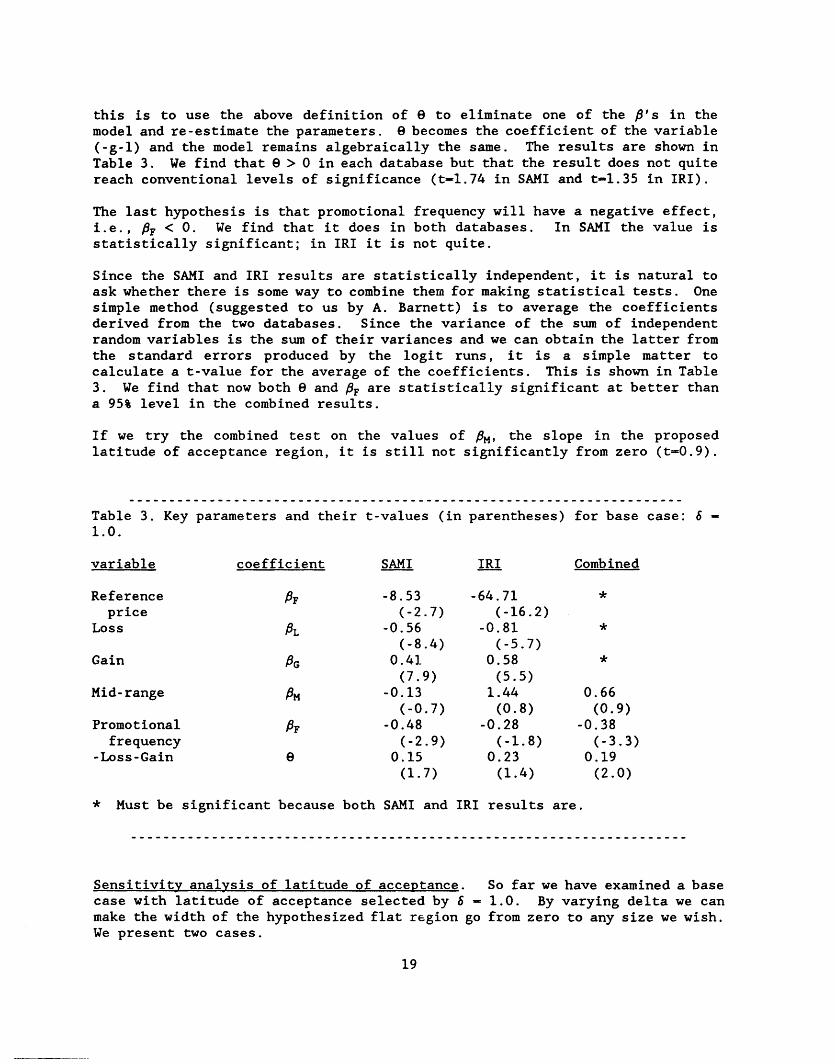
this is to use the above definition of to eliminate one of the 's in themodel and re-estimate the parameters. e becomes the coefficient of the variable(-g-l) and the model remains algebraically the same. The results are shown inTable 3. We find that 8 > 0 in each database but that the result does not quitereach conventional levels of significance (t-1.74 in SAMI and t-1.35 in IRI).

The last hypothesis is that promotional frequency will have a negative effect,i.e., F < . We find that it does in both databases. In SAMI the value isstatistically significant; in IRI it is not quite.

Since the SAMI and IRI results are statistically independent, it is natural toask whether there is some way to combine them for making statistical tests. Onesimple method (suggested to us by A. Barnett) is to average the coefficientsderived from the two databases. Since the variance of the sum of independentrandom variables is the sum of their variances and we can obtain the latter fromthe standard errors produced by the logit runs, it is a simple matter tocalculate a t-value for the average of the coefficients. This is shown in Table3. We find that now both 8 and OF are statistically significant at better thana 95% level in the combined results.

If we try the combined test on the values of M, the slope in the proposedlatitude of acceptance region, it is still not significantly from zero (t=0.9).

Table 3. Key parameters and their t-values (in parentheses) for base case: 6 -1.0.

variable coefficient SAMI IRI Combined

Reference OF -8.53 -64.71 *price (-2.7) (-16.2)

Loss OL -0.56 -0.81 *(-8.4) (-5.7)

Gain PG 0.41 0.58 *

(7.9) (5.5)Mid-range OM -0.13 1.44 0.66

(-0.7) (0.8) (0.9)Promotional OF -0.48 -0.28 -0.38

frequency (-2.9) (-1.8) (-3.3)-Loss-Gain e 0.15 0.23 0.19

(1.7) (1.4) (2.0)

* Must be significant because both SAMI and IRI results are.

Sensitivity analysis of latitude of acceptance. So far we have examined a basecase with latitude of acceptance selected by 6 - 1.0. By varying delta we canmake the width of the hypothesized flat region go from zero to any size we wish.We present two cases.

19

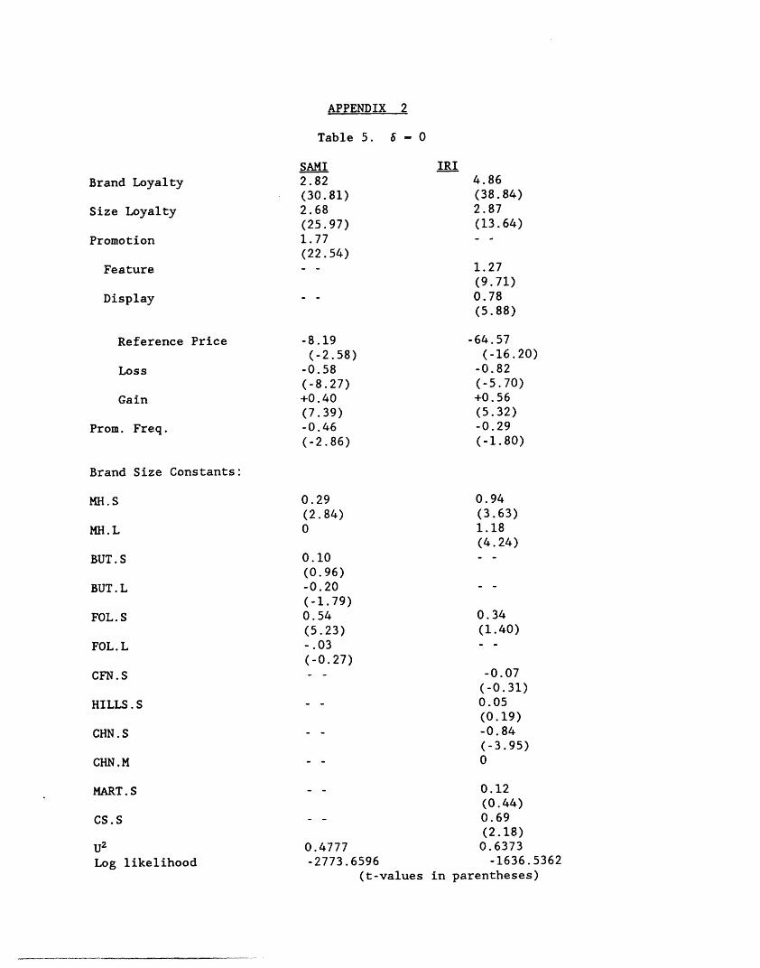
6 - 0. This case eliminates the latitude of acceptance so that theprice model reduces to two segments, one for gains and one for losses. Thecoefficients of interest appear in Table 4 and a complete set in Appendix 2.Excepting the omitted PM, we see that all hypotheses are supported, if not inboth databases separately, then in the combined results.

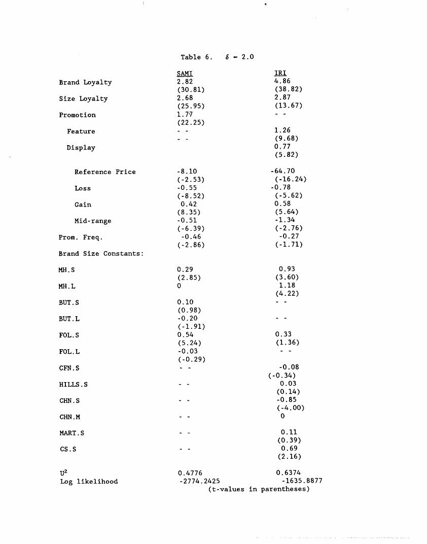
6 - 2.0. Now we have a wide value for the proposed latitude. Therelevant coeffients again appear in Table 4 and the complete set in Appendix 2.Setting aside latitude of acceptance for the moment, we see that all the otherhypotheses are supported, if not in both databases, then in the combinedresults, with the exception of > 0, which does not quite make statisticalsignificance.

The interesting point, however, is that slope, M, of price deviations in themid-range within the proposed latitude of acceptance is now significantlynegative in both databases. This suggests that we are trying to extend thelatitude too far: While the construct was supported at a tighter width (6 =

1.0), it is rejected at the larger width (6 - 2.0).

Table 4. Sensitivity analysis on width of latitude of acceptance: Keyparameters and their t-values (in parentheses) for 6 0 and 6 - 2.0.

6 0 6 =2.0

var. coef. SAMI IRI ave. SAMI IRI ave.

Ref. PF -8.19 -64.57 * -8.10 -64.70 *price (-2.6) (-16.2) (-2.5) (-16.3)Loss PL -0.58 -0.82 * -0.55 -0.78 *

(-8.3) (-5.7) (-8.5) (-5.6)Gain PG 0.40 0.56 * 0.42 0.58 *

(7.4) (5.3) (8.4) (5.6)Mid- fim - - - -0.51 -1.34 *range (-6.4) (-2.8)Prom. PF -0.46 -0.29 -0.38 -0.46 -0.27 -0.37freq. (-2.9) (-1.8) (-3.3) (-2.9) (-1.7) (-3.2)-Loss e 0.18 0.26 0.22 0.13 0.20 0.17-Gain (2.1) (1.5) (2.3) (1.7) (1.2) (1.8)

* Must be significant because both SAMI and IRI results are.

To gain a better understanding of the width of the latitude of acceptance wehave performed an exploration of 6 beyond the three cases discussed above. Wefind a price-insensitive region (slope not significant) around the referenceprice, but the slope depends on how wide we make the interval. As the width,6, moves away from zero, the region remains insensitive to price for 6 up toabout 1.0. As the width increases further toward 6 - 2.0, price sensitivitybecomes evident (magnitude of slope significant).

20

DISCUSSSION

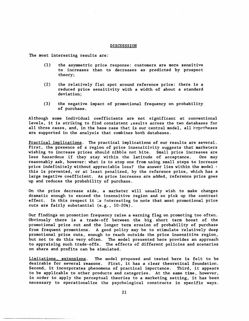
The most interesting results are:

(1) the asymmetric price response: customers are more sensitiveto increases than to decreases as predicted by prospecttheory;

(2) the relatively flat spot around reference price: there is areduced price sensitivity with a width of about a standarddeviation;

(3) the negative impact of promotional frequency on probabilityof purchase.

Although some individual coefficients are not significant at conventionallevels, it is striking to find consistent esults across the two databases forall three cases, and, in the base case that is our central model, all bypcthesesare supported in the analysis that combines both databases.

Practical implications. The practical implications of our results are several.First, the presence of a region of price insensitivity suggests that marketerswishing to increase prices should nibble not bite. Small price increases areless hazardous if they stay within the latitude of acceptance. One mayreasonably ask, however: what is to stop one from using small steps to increaseprice indefinitely without appreciable loss? the answer lies within the model -this is prevented, or at least penalized, by the reference price, which has alarge negative coefficient. As price increases are added, reference price goesup and reduces the probability of purchase.

On the price decrease side, a marketer will usually wish to make changesdramatic enough to exceed the insensitive region and so pick up the contrasteffect. In this respect it s interesting to note that most promotional pricecuts are fairly substantial (e.g., 10-20%).

Our findings on promotion frequency raise a warning flag on promoting too often.Obviously there is a trade-off between the big short term boost of thepromotional price cut and the longer term erosion of probability of purchasefrom frequent promotions. A good policy may be to stimulate relatively deeppromotional price cuts, enough to reach outside the price insensitive region,but not to do this very often. The model presented here provides an approachto appraising such trade-offs. The effects of different policies and scenarioson share and profits can be simulated.

Limitations, extensions. The model proposed and tested here is felt to bedesirable for several reasons. First, it has a clear theoretical foundation.Second, it incorporates phenomena of practical importance. Third, it appearsto be applicable to other products and categories. At the same time, however,in order to apply the perceptual theories to a marketing setting, it has beennecessary to operationalize the psychological constructs in specific ways.

21

III

These are not unique and other researchers may find better ones. Our resultsare generally encouraging, but a single application, even on two databases,cannot be considered definitive. More testing would certainly be desirable,especially on other product categories.

Several elaborations suggest themselves immediately: Perhaps the latitude ofacceptance region is asymmetric. It would be interesting to try more segmentsin the price response function. Quite likely there are interactions with othermarketing variables, for example, feature advertising. These and certain otherinvestigations lie beyond the limits of the present data sets but some of themshould become feasible in the larger scanner panel databases now coming intoexistence.

REFERENCES

Ben Akiva, Moshe and Steven R. Lerman (1985), Discrete Choice Analysis, The MITPress, Cambridge, MA.

Dodson, Joe A., Alice Tybout, and Brian Sternthal. (1978), "Impact of Deals andDeal Retraction on Brand Switching," Journal of Marketing Research, 15, 72-78.

Emery, F. E., (1970), "Some Psychological Aspects of Price," in Bernard Taylorand Gordon Wills (eds.), Pricing Strategy (Princeton, N. J.:Brandon/Systems)112-131.

Friedman, B.M. (1979), "Optimal Expectations and the extreme Information ofRational Expectations' Macromodels," Journal of Monetary Economics, 5, 23-41.

Gabor, Andre and C. W. J. Granger (1966), "Price as an Indicator of Quality:Report of an Enquiry," Economica, 46, February, 43-70.

Gensch, D. H. and W. W Recker, (1979), "The Multinomial Multiattribute LogitChoice Model," Journal of Marketing Research, February, 124-132.

Guadagni, Peter M. and John D. C. Little (1983), "A Logit Model of Brand ChoiceCalibrated on Scanner Data," Marketing Science, 2, Summer, 203-238.

Hauser, John R. (1978), "Testing the Accuracy, Usefulness, and Significance ofProbabalistic Choice Models: An Information Theoretic Approach," OperationsResearch, 26 (May), 406-421.

Helson, H., (1964), Adaptation-Level Theory, (New York: Harper and Row).

Kahneman, Daniel and Amos Tversky, (1979) "A Prospect theory: an analysis ofdecision under risk." Econometrica, 47 (March), 263-291.

Kalwani, Manohar, Heikki J. Rinne, Yoshi Sugita and Chi-Kin Yim (1988), "AReference Price Based Model of Consumer Brand Choice," Kannert Graduate Schoolof Management Working Paper No. 935, Purdue University.

22

Lattin, James M. and Randolph E. Bucklin (1987), "The Dynamics of ConsumerResponse to Price Discounts," Working Paper, Graduate School of Business,Stanford University.

Monroe, Kent B. (1971), "Measuring Price Thresholds by Psychophysics andLatitudes of Acceptance," Journal of Marketing Research, 8, November, 460-4.

(1973), "Buyers' Subjective Perceptions of Price." Journal ofMarketing Research, 10, February, 70-80.

------------ (1976), " The Influence of Price Differences and Brand Familiarityon Brand Preferences," Journal of Consumer Research, 3, June, 42-49.

Pessemier, E. A. (1960), "An Experimental Method for Estimating Demand," Journalof Business, 33, October, 373-383.

Raman, K. and F. M. Bass (1988), "A General Test of Reference Price Theory inthe Presence of Threshold Effects," working paper, University of Texas at Dallas

Rinne, Heikki J. (1981), "An Empirical Investigation of the Effects of ReferencePrices on Sales," Doctoral dissertation, Purdue University.

Sawyer, Alan G. and Peter R. Dickson (1984), "Psychological Perspectives onConsumer Response to Sales Promotion," in Katharine E. Jocz, ed., Research onSales Promotion: Collected Papers, Marketing Science Institute, Cambridge, MA.

Sherif, Carolyn W. (1963), "Social Categorization as a Function of Latitude ofAcceptance and Series Range," Journal of Abnormal Psychology, 67, 148-156.

Sherif, Muzafer and Carl I. Hovland (1961), Social Judgment, Yale UniversityPress, New Haven

Sherif, Muzafer, Daniel Taub and Carl I. Hovland (1958), "Assimilation andContrast Effects of Anchoring Stimuli on Judgments," Journal of ExperimentalPsychology, 55, No. 2, 150-155.

Shoemaker, Robert W. and F. Robert Shoaf (1977), "Repeat Rates of DealPurchases," Journal of Advertising Research, 17, 47-53.

Thaler, Richard (1985), "Mental Accounting and Consumer Choice," MarketingScience, 4, Summer, 199-214.

Uhl, J.N. and H. L. Brown (1971), "Consumer Perception of Experimental RetailFood Price Changes," The Journal of Consumer Affairs, 5, Winter, 174-185.

Winer, Russell S. (1986), "A Reference Price Model of Brand Choice forFrequently Purchased Products," Journal of Consumer Research, 13, September,250-256.

23

APPENDIX 1

Replot of data from Sherif. Taub and Hovland (1958)

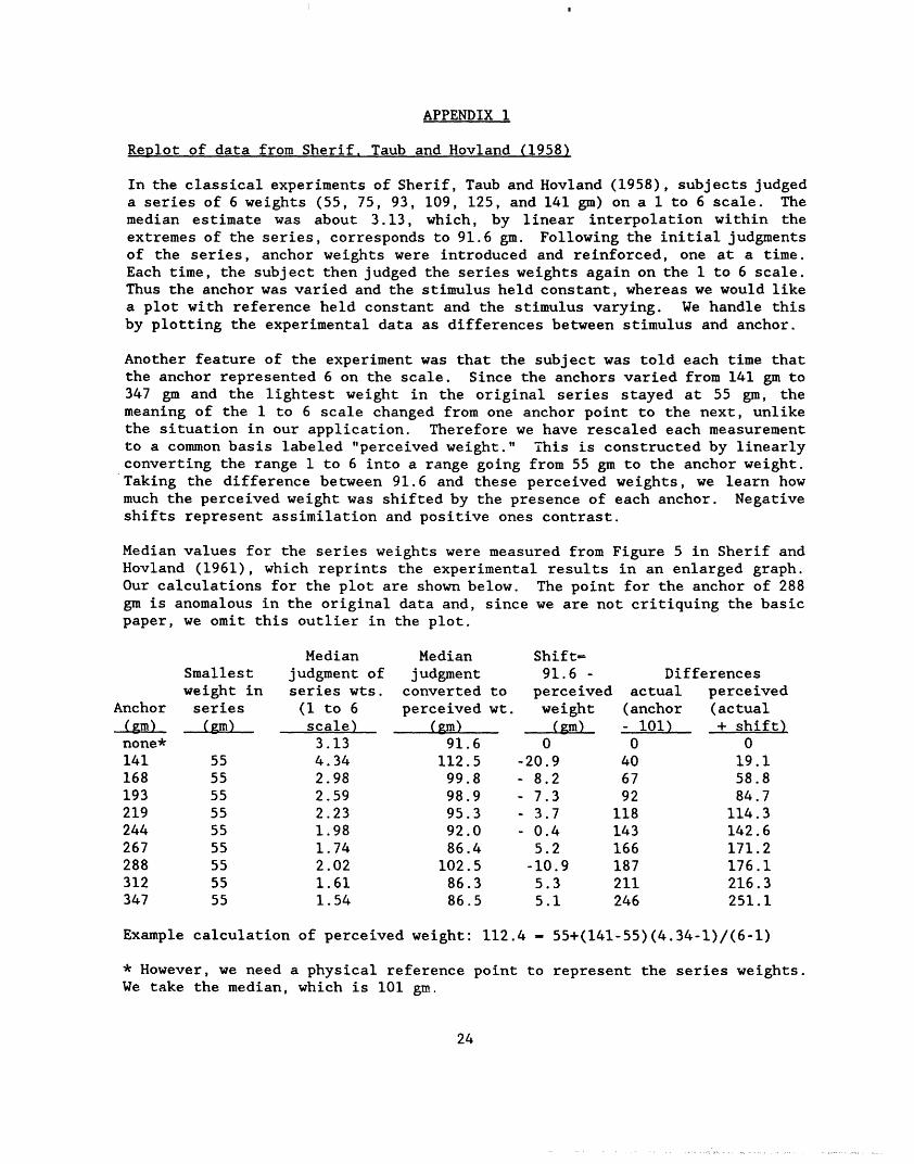
In the classical experiments of Sherif, Taub and Hovland (1958), subjects judgeda series of 6 weights (55, 75, 93, 109, 125, and 141 gm) on a 1 to 6 scale. Themedian estimate was about 3.13, which, by linear interpolation within theextremes of the series, corresponds to 91.6 gm. Following the initial judgmentsof the series, anchor weights were introduced and reinforced, one at a time.Each time, the subject then judged the series weights again on the 1 to 6 scale.Thus the anchor was varied and the stimulus held constant, whereas we would likea plot with reference held constant and the stimulus varying. We handle thisby plotting the experimental data as differences between stimulus and anchor.

Another feature of the experiment was that the subject was told each time thatthe anchor represented 6 on the scale. Since the anchors varied from 141 gm to347 gm and the lightest weight in the original series stayed at 55 gm, themeaning of the 1 to 6 scale changed from one anchor point to the next, unlikethe situation in our application. Therefore we have rescaled each measurementto a common basis labeled "perceived weight." This is constructed by linearlyconverting the range 1 to 6 into a range going from 55 gm to the anchor weight.Taking the difference between 91.6 and these perceived weights, we learn howmuch the perceived weight was shifted by the presence of each anchor. Negativeshifts represent assimilation and positive ones contrast.

Median values for the series weights were measured from Figure 5 in Sherif andHovland (1961), which reprints the experimental results in an enlarged graph.Our calculations for the plot are shown below. The point for the anchor of 288gm is anomalous in the original data and, since we are not critiquing the basicpaper, we omit this outlier in the plot.

Smallestweight inseries

(gm)

555555555555555555

Medianjudgment ofseries wts.(1 to 6scale)3.134.342.982.592.231.981.742.021.611.54

Median Shiftsjudgment 91.6 - Differencesconverted to perceived actual perceivedperceived wt. weight (anchor (actual

(g m) (gm) - 101) + shift)91.6 0 0 0

112.5 -20.9 40 19.199.8 - 8.2 67 58.898.9 - 7.3 92 84.795.3 - 3.7 118 114.392.0 - 0.4 143 142.686.4 5.2 166 171.2

102.5 -10.9 187 176.186.3 5.3 211 216.386.5 5.1 246 251.1

Example calculation of perceived weight: 112.4 - 55+(141-55)(4.34-1)/(6-1)

* However, we need a physical reference point to represent the series weights.We take the median, which is 101 gm.

24

Anchor

(gm)none*141168193219244267288312347

Brand Loyalty

Size Loyalty

Promotion

Feature

APPENDIX 2

Table 5. 6 - 0

SAMI2.82(30.81)2.68(25.97)1.77(22.54)

IRI

Display

Reference Price

Loss

Gain

Prom. Freq.

-8.19(-2.58)

-0.58(-8.27)+0.40

(7.39)-0.46(-2.86)

4.86(38.84)2.87(13.64)

1.27

(9.71)0.78(5.88)

-64.57(-16.20)

-0.82(-5.70)+0.56

(5.32)-0.29(-1.80)

Brand Size Constants:

MH.S

MH. L

BUT. S

BUT.L

FOL.S

FOL. L

CFN.S

HILLS.S

CHN.S

CHN.M

MART. S

CS.S

U2

Log likelihood

0.29(2.84)0

0.10(0.96)-0.20(-1.79)0.54(5.23)-.03

(-0.27)

0.94(3.63)1.18(4.24)

0.34(1.40)

-0.07

(-0.31)0.05(0.19)-0.84(-3.95)0

- - 0.12(0.44)0.69(2.18)

0.4777 0.6373-2773.6596 -1636.5362

(t-values in parentheses)

Brand Loyalty

Size Loyalty

Promotion

Feature

Display

Reference Price

Loss

Gain

Mid-range

Prom. Freq.

Brand Size Constants:

MH.S

MH.L

BUT. S

BUT. L

FOL.S

FOL.L

CFN.S

HILLS.S

CHN.S

CHN.M

MART. S

CS.S

U2

Log likelihood

Table 6.

SAMI2.82(30.81)2.68(25.95)1.7'7(22.25)

-8.10(-2.53)-0.55(-8.52)0.42(8.35)-0.51(-6.39)-0.46

(-2.86)

0.29(2.85)0

0.10(0.98)-0.20(-1.91)0.54(5.24)-0.03

(-0.29)

6 - 2.0

IRI4.86(38.82)2.87(13.67)

1.26(9.68)0.77(5.82)

-64.70(-16.24)

-0.78(-5.62)0.58(5.64)-1.34(-2.76)-0.27

(-1.71)

0.93(3.60)1.18(4.22)

0.33(1.36)

-0.08(-0.34)

0.03(0.14)-0.85(-4.00)0

0.11

(0.39)0.69(2.16)

0.4776 0.6374-2774.2425 -1635.8877

(t-values in parentheses)