University of Pennsylvania University of Pennsylvania

ScholarlyCommons ScholarlyCommons

Marketing Papers Wharton Faculty Research

9-2008

A Price Discrimination Model of Trade Promotions A Price Discrimination Model of Trade Promotions

Tony Haitao Cui University of Pennsylvania

Jagmohan S. Raju University of Pennsylvania

Z John Zhang University of Pennsylvania

Follow this and additional works at: https://repository.upenn.edu/marketing_papers

Part of the Marketing Commons

Recommended Citation Recommended Citation Cui, T., Raju, J. S., & Zhang, Z. (2008). A Price Discrimination Model of Trade Promotions. Marketing Science, 27 (5), 779-795. http://dx.doi.org/10.1287/mksc.1070.0314

This paper is posted at ScholarlyCommons. https://repository.upenn.edu/marketing_papers/199 For more information, please contact repository@pobox.upenn.edu.

A Price Discrimination Model of Trade Promotions A Price Discrimination Model of Trade Promotions

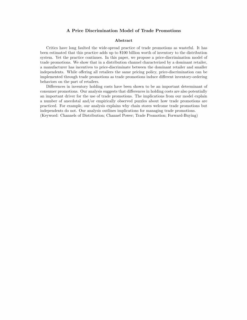
Abstract Abstract Critics have long faulted the wide-spread practice of trade promotions as wasteful. It has been estimated that this practice adds up to $100 billion worth of inventory to the distribution system. Yet, the practice continues. In this paper, we propose a price discrimination model of trade promotions. We show that in a distribution channel characterized by a dominant retailer, a manufacturer has incentives to price discriminate between the dominant retailer and smaller independents. While offering all retailers the same pricing policy, price discrimination can be implemented through trade promotions because they induce different inventory-ordering behaviors on the part of retailers.

Differences in inventory holding costs have been shown to be an important determinant of consumer promotions. Our analysis suggests that differences in holding costs are also potentially an important driver for the use of trade promotions. The implications from our model explain a number of anecdotal and/or empirically observed puzzles about how trade promotions are practiced. For example, our analysis explains why chain stores welcome trade promotions but independents do not. Our analysis outlines implications for managing trade promotions.

Keywords Keywords channels of distribution, channel power, trade promotion, forward buying

Disciplines Disciplines Business | Marketing

This journal article is available at ScholarlyCommons: https://repository.upenn.edu/marketing_papers/199

A Price Discrimination Model of TradePromotions

Tony Haitao Cui Jagmohan S. Raju Z. John Zhang¤

May 2007

Forthcoming, Marketing Science

¤The authors thank the editor, the area editor and three reviewers for their thoughtful comments. Tony Haitao Cuiis an Assistant Professor of Marketing at the Carlson School, University of Minnesota. Jagmohan S. Raju is JosephJ. Aresty Professor of Marketing at the Wharton School. Z. John Zhang is a Professor of Marketing at the WhartonSchool. Email correspondence: tcui@umn.edu, rajuj@wharton.upenn.edu, and zjzhang@wharton.upenn.edu.

A Price Discrimination Model of Trade Promotions

Abstract

Critics have long faulted the wide-spread practice of trade promotions as wasteful. It hasbeen estimated that this practice adds up to $100 billion worth of inventory to the distributionsystem. Yet the practice continues. In this paper, we propose a price-discrimination model oftrade promotions. We show that in a distribution channel characterized by a dominant retailer,a manufacturer has incentives to price-discriminate between the dominant retailer and smallerindependents. While o®ering all retailers the same pricing policy, price-discrimination can beimplemented through trade promotions as trade promotions induce di®erent inventory-orderingbehaviors on the part of retailers.Di®erences in inventory holding costs have been shown to be an important determinant of

consumer promotions. Our analysis suggests that di®erences in holding costs are also potentiallyan important driver for the use of trade promotions. The implications from our model explaina number of anecdotal and/or empirically observed puzzles about how trade promotions arepracticed. For example, our analysis explains why chain stores welcome trade promotions butindependents do not. Our analysis outlines implications for managing trade promotions.(Keyword: Channels of Distribution; Channel Power; Trade Promotion; Forward-Buying)

1. Introduction

According to the most recent estimate, consumer goods manufacturers in US spend about $85 billion

on trade promotions amounting to 13% of sales. In comparison, consumer promotions account for

6%, and advertising and media spending only 4% of sales (Cannondale Associates 2002). Although

trade promotions are widely used by manufacturers, they are often seen as wasteful. For example,

Buzzell, Quelch, and Salmon (1990) argue that trade promotions impose severe administrative

burdens on manufacturers and add huge inventory costs to distribution channels.1

Many have asked the question that if trade promotions are indeed ine±cient, why are man-

ufacturers still using them? A number of explanations have been proposed in the literature. It

has been suggested that manufacturers face a Prisoners' Dilemma like situation { they have to

o®er trade promotions, otherwise the competition will take business away from them (e.g., Drμeze

and Bell 2003). Lal (1990) shows that national brand manufacturers could use trade promotions

to limit the encroachment from a store brand. Lal, Little, and Villas-Boas (1996) suggest that

allowing retailers to forward buy bene¯ts competing manufacturers since forward buying decreases

the intensity of competition between manufacturers. Agrawal (1996) analyzes the role of brand

loyalty in determining optimal advertising policy (defensive strategy to build brand loyalty) and

trade promotion policy (o®ensive strategy to steal customers from competition).

In this paper, we o®er another explanation for trade promotions. Our explanation essentially

establishes the price discrimination role of trade promotions in a channel context: manufacturers can

use trade promotions to price discriminate between large retailers (e.g., chains) and small retailers

(e.g., independents) by exploiting their di®erent inventory carrying costs. Blattberg, Eppen, and

Lieberman (1981) have shown that retailers can take advantage of the di®erences in consumers'

inventory carrying costs. In this paper we show that manufacturers can similarly take advantage

of the di®erences in retailers' inventory holding costs to achieve price discrimination through trade

1According to one estimate, $75-$100 billion worth of inventory is added into US distribution channel because oftrade promotions. See Kahn and McAlister, 1997, page 21.

1

promotions.

However, price discrimination in a channel context is not a straightforward extension of that

in a non-channel context, as multiple channel members are now involved in pricing and inventory

decisions. More importantly, this price discrimination explanation for trade promotions results

in a number of interesting predictions that are consistent with some of the otherwise puzzling

observations in the area of trade promotions. For example, the predictions from our analysis

explain why:

1. Manufacturers schedule their trade promotions well ahead to make it possible for retailers to

plan forward buying.

2. Trade promotions are observed for packaged goods but not for perishable goods (Sellers 1992).

3. Chain stores are happier with trade promotions but independent and convenience stores not.2

4. Manufacturers allow forward buying but forbid diverting.

5. Manufacturers are complaining much more about trade promotions in recent years.

We believe that our ability to explain all these in the context of a parsimonious model suggests that

the model is potentially useful. More speci¯cally, in the context of a channel consisting of a single

manufacturer and multiple retailers, we show that a manufacturer can e®ectively price discriminate

among retailers by o®ering trade promotions if retailers have di®erent inventory holding costs. The

stores with lower holding costs and higher warehouse capacity (usually dominant retailers like chain

stores and warehouse clubs) can bene¯t from forward buying. Interestingly, we further show that

not only does the retailer with low holding costs bene¯t from trade promotions, but the retailer

2Independents and wholesalers who act as buying agents for independents always complain that trade promotionsare not a fair practice for them (Zwiebach 1990, U.S. Distribution Journal 1992). For example, \Not surprisingly, ina broad survey of wholesalers, 87 percent agreed that the most urgent issue facing the wholesale-supplied system isfair and equal access to trade promotion funds." (U.S. Distribution Journal 1993b). On the other hand, chain storesbene¯t more from trade promotions and are happy with trade promotions (Progressive Grocer 2002, U.S. DistributionJournal 1993a). For instance, \Results also noted in the study show that wholesalers and their independent retailcustomers tend to bene¯t less from trade allowance programs than do other distribution channels." (U.S. DistributionJournal 1993a).

2

with high holding costs can also bene¯t from this practice. Indeed, social welfare can also increase.

Although we initially derive these results in a dominant retailer channel setting (Samuelson and

Nordhaus 1989), we show in the technical appendix accompanying this paper (available on the

Website of this journal) that these results hold in a more general competitive channel setting also.

To the extent that a manufacturer can use trade promotions to price discriminate between re-

tailers, Jeuland and Narasimhan (1985) is closely related to our study. However, our research di®ers

from theirs. In their model, the retailers are not making pricing decisions.3 We explicitly model

retailers' pricing decisions over time. Our model therefore takes the Jeuland and Narasimhan's

analysis to the next logical step. This generalization yields interesting insights. One of these in-

sights is that trade promotions can alleviate the double marginalization problem by giving the

leading retailer more incentives to charge a lower retail price.4 5 In addition, the model allows us

to make some testable predictions about the practice of trade promotions.

The rest of the paper is organized as follows. The next section describes the dominant retailer

model. The analysis in Section 3 consists of two parts. The ¯rst part outlines the benchmark case

where the manufacturer is not allowed to o®er trade promotions and analyzes the manufacturer's

incentives to price discriminate between a dominant retailer and the competitive fringe. The second

part derives the manufacturer's optimal trade promotion strategies and the retailers' optimal pricing

and inventory decisions. Section 4 derives a number of interesting predictions regarding the e®ect

of trade promotions on the manufacturer's pro¯ts, retailers' pro¯ts, and social welfare. Section 5

relaxes some assumptions used in the model. We conclude with a summary in Section 6.

3In Jeuland and Narasimhan (1985), a seller could price discriminate between more intensely consuming and lessintensely consuming customers by o®ering temporary price cuts. In order to make this section consistent with therest of the paper, we are using \manufacturer" and \retailers" as in the rest of paper to represent the \seller" and\customers" in Jeuland and Narasimhan (1985), respectively. We thank anonymous Reviewer 3 for the suggestion.

4Double marginalization problem refers to the situation where the economic interests of upstream and downstream¯rms are not aligned such that the retail price facing end users is too high to maximize channel pro¯ts, as illustratedin Jeuland and Shugan (1983).

5Bruce, Desai and Staelin (2005) show that manufacturers of more durable products give deeper promotionaldiscounts, which helps mitigate the double-marginalization problem. One of the di®erences between our research andtheirs is that our research shows manufacturers can use trade promotions to alleviate double-marginalization throughprice discriminating between retailers. Their research shows that manufacturers selling a more durable product o®era greater depth of trade promotions and therefore have a less sever double marginalization problem.

3

2. The Model

Consider a stylized channel where a manufacturer is selling a product through a dominant retailer

(e.g., a chain store) and the competitive fringe (e.g., smaller independent retailers). The dominant

retailer sets the retail price (p), and the competitive fringe takes the retail price as the market price

(Samuelson and Nordhaus 1989).6 We start with the dominant retailer model for three reasons.

First, the phenomenon of \power retailers" is a familiar scene in today's retailing landscape and

large retailers are becoming increasingly dominant in the marketplace.7 8 Second, large chains

often assume the role of price leadership and exert pricing in°uence over smaller retailers (Raju

and Zhang 2005). Third, the dominant retailer model simpli¯es the expositions considerably. As

we show in Technical Appendix, if we were to relax the key assumption of only the dominant

retailer setting the retail price and introduce price competition, our conclusions will not change

qualitatively.9

The total market demand in each period is given by Q = a ¡ bp, where a > 0 and b > 0 are

constants. The dominant retailer faces a downward-sloping demand function given by

Qd = a¡ b1p: (2.1)

6Formally, the competitive fringe supplies at the quantity where the price equals the (rising) marginal cost.7In the grocery industry, for example, mass merchandisers, warehouse clubs, and chain stores account for 23% of

total grocery sales in 2002, while that number was only 9% in 1995 (The McKinsey Quarterly 2003). Furthermore,the number of grocery chain stores in the U.S. was 18,400 in 1980, accounting for 52.7% of the total number of grocerystores. By 2003, the number of chain stores has mushroomed to 21,560 accounting for 65.4% of the total number ofgrocery stores. In the meantime, the share of dollar sales for chain stores increases from about 60.2% to 82.7%. Notsurprisingly, Independents shrank in number from 16,500 in 1980 to 11,421 in 2003 and their dollar sales percentagedecreased from 39.8% to 17.3% (Progressive Grocer Annual Report 1981, 2003).

8There are several recent papers studying how the emergence of dominant retailers a®ects the interactions betweenchannel members. In a bargaining model, Dukes, Gal-Or, and Srinivasan (2006) show that manufacturers may bene¯tfrom the increase in retailer dominance since channel e±ciency can improve with dominant retailers gaining costadvantages. Geylani, Dukes, and Srinivasan (2005) show that a manufacturer has an incentive to engage in jointpromotions and advertising with weaker retailers since the manufacturer gets a higher margin with weaker retailersthan with dominant retailers, who has the power to dictate the wholesale price.

9In some industries, small stores can form cooperatives such as buying clubs to get promotional discounts frommanufacturers or can make purchases from a middle party like a wholesaler, who buys from manufacturers for manysmall stores. The former case can be analyzed using the competitive model in Technical Appendix TA. The currentpaper is limited in analyzing the later case since we do not model a wholesaler between the manufacturer and retailers.

4

The demand facing the competitive fringe in each period is correspondingly, 10

Qc = Q¡Qd = (b1 ¡ b)p: (2.2)

In this dominant retailer channel, the competitive fringe's demand is increasing in retail price p

while the dominant retailer's is decreasing in p such that these two di®erent types of retailers do

compete with each other. Figure 1 illustrates the demand functions at the retail level. We assume

b < b1 · 3b2 in our analysis to avoid any corner solution.

Q

p

a/b

a/b1

a

Q = a – b pQ

d = a – b1 pQ c

= (b

1–

b)p

0

Figure 1: Retailers' Demands for b < b1 · 1:5b

In this channel, all retailers incur a holding cost for any inventory carried from one period to

the next. In practice, chain stores and warehouse clubs usually have lower inventory costs than

independents. One reason could be a lower cost of capital. Further, chain stores and warehouse

clubs also have higher inventory holding capacity and much more shelf space than independents,

a big component of inventory holding costs, especially for food retailers (Blattberg, Eppen and

Lieberman 1981). Therefore, it is reasonable to assume a lower inventory holding cost for the dom-

inant retailer.11 We assume that the dominant retailer has a ¯nite unit holding cost (0 · h1 <1)10It is worthy of noting that the competitive fringe in this paper is considered as a group of independents that is

modeled as a single entity. Each independent in the competitive fringe is weak in terms of market power comparedwith the single dominant retailer. We thank anonymous Reviewer 3 for suggesting to make this point clear.11Further, in Appendix A we also show that the dominant retailer has more incentives than retailers in the

competitive fringe to reduce unit holding cost rate, since the economic reward from a unit of reduction in holding

5

and retailers in the competitive fringe have an in¯nite unit holding cost (h2 = 1). It is impor-

tant to note that the in¯nite inventory holding cost for a competitive fringe is only a simplifying

assumption, and we relax the assumption in Technical Appendix where we allow a ¯nite di®erence

in the inventory holding costs between the dominant retailer and retailers from the competitive

fringe. As the manufacturer's production costs do not a®ect our substantive conclusions, we set

them equal to zero for simplicity.

Manufacturer's Decision Variables: The manufacturer in our model announces a wholesale

price wi for each period i within a pricing cycle consisting of N periods (i = 1; :::;N).12 The length

of the pricing cycle N is also a manufacturer decision variable. The manufacturer's objective is to

maximize the average pro¯t per period within a pricing cycle.13

Dominant Retailer's Decision Variables: Conditional on the manufacturer's decisions on the

length of a pricing cycle (N) and the wholesale prices in each period within the cycle (w1; w2; :::; wN ),

the dominant retailer sets the retail price pi for periods i = 1; 2; :::;N to maximize its total pro¯t in

each pricing cycle. As the dominant retailer has a ¯nite holding cost, some inventory may be carried

from one period to the next if forward buying is pro¯table. Therefore, the dominant retailer also

makes decisions on Qi;jd , the inventory the dominant retailer orders in period i and sells in period

j, where i; j 2 f1; :::; Ng and i · j.

Competitive Fringe's Decision Variables: Retailers in the competitive fringe take pi as the

market price in each period i. As the holding cost for these retailers is assumed to be in¯nite, they

do not carry any inventory from one period to the next. Therefore, a retailer in the competitive

fringe will buy the product from the manufacturer and sell to customers if wi · pi in period i.cost rate is higher for the dominant retailer who makes forward buying than for the competitive fringe. Therefore,the dominant retailer will have a lower unit holding cost than the competitive fringe in the long run, which furthervalidates our assumption.12In this paper, we are modeling o®-invoice trade promotions.13For an early proof for the equivalence between maximizing average pro¯t per period and maximizing total pro¯t

as discount factor approaches zero, see Jewell (1963).

6

Mathematically, the manufacturer solves the following optimization problem

maxw1;w2;:::;wN ;N

"PNi=1wi(

PNj=iQ

i;jd +Qi;ic )

N

#;

where Qi;jd denotes the inventory the dominant retailer orders in period i and sells in period j,

and Qi;ic the inventory the retailers in the competitive fringe order and sell in period i. Of course,

we have Qi;jc = 0 for any i6= j, as a competitive fringe does not carry any inventory. Given the

manufacturer's wholesale prices and the length of pricing cycle (w1; w2; :::; wN ; N), the dominant

retailer's optimization is given by

maxp1;p2;:::;pN ;Qi;j

d

24 NXj=1

jXi=1

[pj ¡ wi ¡ h1(i¡ 1)]Qi;jd35 :

We summarize the timing of decisions in this channel in Figure 2.

Manufacturer decides:the length of pricing cycle and wholesale

prices for each period over the cycle

Dominant retailer and the competitive fringe

decide: how much to purchase from the manufacturer

Dominant retailer sets the retail price

Competitive fringe meets the residual

demand

Figure 2: Timing of Decisions in Dominant Retailer Channel

The model speci¯ed above can result in a number of di®erent pricing outcomes. Figure 3 illus-

trates several possible optimal wholesale price schedules. We de¯ne trade promotions as temporary

price discounts o®ered by the manufacturer to retailers. Therefore, all the schedules except Case

(a) in Figure 3 could be viewed as trade promotion schedules. For instance, in Figure 3(b), w1 is

the discounted wholesale price and w2 is the regular wholesale price. If the manufacturer o®ers a

low price in one period and charges higher and increasing prices for the following two periods as in

3(d), then w1 and w2 are both promotional wholesale prices and w3 is the regular wholesale price.

7

-

6

-

6

-

6

-

6

time(periods)

wholesale price

time(periods)

wholesale price

time(periods)

wholesale price

time(periods)

wholesale price

1 2 3 4 ... 1 2

1 2 3 1 2 3

(a) (b)

(c) (d)

w1 w2 w3 w4 :::

w1

w2

w1

w2 w3

w1

w2

w3

One Pricing Cycle¾ -

wholesale price

Figure 3: Examples of Optimal Wholesale Price Schedules

3. Analysis

We ¯rst show why the manufacturer has an incentive to price discriminate. We analyze the manu-

facturer's and the dominant retailer's pricing decisions, assuming that the manufacturer charges a

time-invariant single wholesale price to all retailers. This case of no trade promotions is our bench-

mark for comparison with the case where the manufacturer o®ers trade promotions to the retailers.

We will show that under some conditions, trade promotions can increase the manufacturer's pro¯ts

as well as channel pro¯ts, even after accounting for the additional inventory costs that are added

into the channel as a consequence of forward buying by the dominant retailer.

3.1 Manufacturer's Incentives to Price Discriminate between Retailers

If the manufacturer does not o®er trade promotions, i.e., that the wholesale price is constant over

time, all retailers will order from the manufacturer in each period and none will carry any inventory

from one period to the next. The optimal prices and pro¯ts are easy to determine, and we simply

state these in Lemma 1.

Lemma 1 If the manufacturer is restricted to o®ering a common time-invariant wholesale price

8

to retailers, then the manufacturer will set its wholesale price at ws =a(2b1¡b)2bb1

and the dominant

retailer sets its retail price at ps =a(2b1+b)4bb1

. The manufacturer's average sales and pro¯t per period

are given by Qs =a(2b1¡b)4b1

and ¦s =a2(2b1¡b)2

8bb21respectively.

Proof of Lemma 1. Please see Appendix B.14

Of course, a single wholesale price is sub-optimal for the manufacturer for two reasons. First,

the competitive fringe is passive in setting the retail price in the channel, and it will meet the

residual demand as long as the wholesale price it has to pay is less or equal to the retail price

set by the dominant retailer. Thus, ideally, the manufacturer wants to be able to charge the

competitive fringe a higher wholesale price equal to the retail price so as to take away all the

pro¯ts from the competitive fringe. Second, the manufacturer must also be mindful of the \double

marginalization" problem dissipating channel pro¯ts because of too high a retail price. As only

the dominant retailer's marginal cost will determine the retail price, if possible the manufacturer

ideally wants to charge a lower wholesale price only to the dominant retailer. Therefore, to alleviate

the double marginalization problem, and to take advantage of the price following behavior in the

channel, it is in the manufacturer's interest to price discriminate between the dominant retailer and

the competitive fringe. However, charging di®erent wholesale prices to di®erent retailers who are

competing in the same market is unlawful. The manufacturer must ¯nd some other mechanisms

to reap the bene¯ts of price discrimination. Trade promotions, or time-variant wholesale prices, is

one such pricing mechanism.

3.2 Trade Promotions as A Mechanism to Price Discriminate

When the manufacturer o®ers trade promotions, it o®ers the same wholesale prices to all retailers.

Thus, nominally, the manufacturer does not price discriminate. However, as inventory holding

costs di®er among retailers, not all retailers can take advantage of trade promotions to the same

degree. The retailers in the competitive fringe do not carry any inventory from one period to

14Unless stated otherwise, proofs for lemmas and propositions are provided in the Appendix at the end of thispaper..

9

the next, as their holding cost is assumed to be in¯nite (relaxed later). The dominant retailer

¯nds it desirable to carry inventory acquired at the promotional wholesale price to those periods

with higher wholesale prices, i.e. to forward buy, if its unit holding cost (0 · h1 < 1) is low

enough. Because it is more pro¯table to buy in promotional periods and carry inventory forward,

the e®ective wholesale prices are lower for the dominant retailer than for the competitive fringe.

Thus, trade promotions enable the manufacturer to price discriminate.

In Lemma 2, we formalize this intuition, stating the manufacturer's and retailers' optimal

strategies when trade promotions are o®ered in the channel.

Lemma 2 If the dominant retailer has a positive unit holding cost (0 < h1 < 1), while the

competitive fringe has an in¯nite unit holding cost (h2 = 1), then the manufacturer will o®er

the lowest wholesale price in the ¯rst period and charge an increasing wholesale price in each of

the following N ¡ 1 periods within any N-period pricing cycle. The promotional wholesale price

w1 in the ¯rst period, the wholesale prices wi in the ith period (2 · i · N), the retail price pj

(1 · j · N), dominant retailer's sales Qdj in the jth period, competitive fringe's sales Qcj in the

jth period, average sales per period Qh1 , and the manufacturer's average pro¯t per period ¦h1 are

respectively given by8>>>>>>>>>>>>>><>>>>>>>>>>>>>>:

w1 =N [4ab1¡2ab¡b1bh1(N¡1)]2b1[b(N+1)+b1(N¡1)]

wi =a+b1w1+b1h1(i¡1)

2b1i = 2; :::; N

pj = a+b1w1+b1h1(j¡1)2b1

j = 1; :::; N

Qdj =a¡b1w1¡b1h1(j¡1)

2 j = 1; :::; N

Qcj =(b1¡b)[a+b1w1+b1h1(j¡1)]

2b1j = 1; :::; N

Qh1 =14b1[4ab1 ¡ 2ab¡ 2bb1w1 ¡ bb1h1(N ¡ 1)]

¦h1 =1N

hw1PNj=1Qdj +

PNi=1wiQci

i; (3.1)

and we also have ½wi = p

i i = 2; :::; Npi ¡ pi¡1 = h1

2 i = 2; :::; N: (3.2)

Figure 4 shows the manufacturer's and the retailer's optimal prices within a pricing cycle when

N is equal to 5. The retail price will be raised by h12 per period, as the dominant retailer's e®ective

10

-

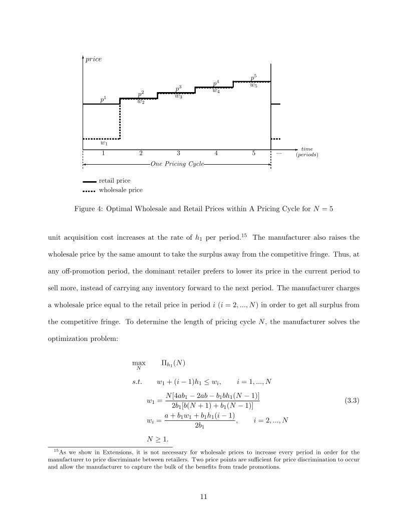
6

time(periods)

price

1 2 3 4 5 ...

w1

w2w3

w4w5

p1p2

p3p4

p5

One Pricing Cycle¾ -

retail price

wholesale price

Figure 4: Optimal Wholesale and Retail Prices within A Pricing Cycle for N = 5

unit acquisition cost increases at the rate of h1 per period.15 The manufacturer also raises the

wholesale price by the same amount to take the surplus away from the competitive fringe. Thus, at

any o®-promotion period, the dominant retailer prefers to lower its price in the current period to

sell more, instead of carrying any inventory forward to the next period. The manufacturer charges

a wholesale price equal to the retail price in period i (i = 2; :::; N) in order to get all surplus from

the competitive fringe. To determine the length of pricing cycle N , the manufacturer solves the

optimization problem:

maxN

¦h1(N)

s:t: w1 + (i¡ 1)h1 · wi; i = 1; :::; N

w1 =N [4ab1 ¡ 2ab¡ b1bh1(N ¡ 1)]2b1[b(N + 1) + b1(N ¡ 1)] (3.3)

wi =a+ b1w1 + b1h1(i¡ 1)

2b1; i = 2; :::; N

N ¸ 1:15As we show in Extensions, it is not necessary for wholesale prices to increase every period in order for the

manufacturer to price discriminate between retailers. Two price points are su±cient for price discrimination to occurand allow the manufacturer to capture the bulk of the bene¯ts from trade promotions.

11

The constraints w1+(i¡ 1)h1 · wi guarantee that the dominant retailer's e®ective unit acqui-

sition cost of the items sold in period i = 2; :::;N is no higher than the wholesale price in the same

period, so that the dominant retailer does not ¯nd it worthwhile to purchase from the manufacturer

in period i at the current wholesale price. As the dominant retailer's e®ective acquisition cost per

unit is increasing at a faster rate (h1 per period) than the wholesale price (h12 per period) over time,

there is an upper limit for N beyond which it is not pro¯table for the dominant retailer to carry any

inventory. The constraints thus provide an upper bound on the manufacturer's decision variable

N . As the range for N is convex and compact, there always exists a solution to the optimization

problem (3.3). Given the optimal N and the sequence of wholesale prices preannounced by the

manufacturer, retailers will not carry any inventory from one pricing cycle to the next since the ¯rst

period in the next pricing cycle will be a promotional period again. The manufacturer's decisions

on N and the sequence of wholesale prices in a pricing cycle will therefore not depend on its deci-

sions in any other pricing cycles. In Appendix C, we show that the manufacturer's announcement

of both the length of pricing cycles N and the sequence of wholesale prices is credible. The man-

ufacturer has no incentive in any period within a pricing cycle to deviate from the preannounced

N and wholesale prices.16 This suggests that both the manufacturer's and retailers' behaviors are

independent between pricing cycles.

It follows from the analysis above that the e®ective unit acquisition cost for the dominant

retailer is lower than that for the competitive fringe in period i = 2; :::; N , or w1 + h1(i¡ 1) < wifor i = 2; :::;N . This leads to our ¯rst Proposition.

Proposition 1 The manufacturer can use trade promotions to price discriminate between retailers

who have di®erent inventory holding costs.

Proposition 1 formally suggests a new justi¯cation for trade promotions not previously recog-

nized in the literature. While o®ering the same wholesale price to all retailers but varying it over

16We thank AE and anonymous Reviewers 1 and 4 for pointing out this to us. In practice, the manufacturer canalso credibly commit to a sequence of prices because of reputation factors, legal factors, etc.

12

time, the manufacturer can price discriminate between retailers who are competing in the same

market, as long as the retailer(s) with high wholesale price sensitivity has lower unit inventory

holding costs than the retailer(s) with low wholesale price sensitivity. Because of the ability to

price discriminate, the manufacturer can pro¯t from trade promotions. This perhaps explains the

paradoxical trend, as noted by Ailawadi, Farris, and Shames (1999), that \at the peak of the trade-

promotion controversy, manufacturers' pro¯ts increased at a fairly steady rate, whereas retailers'

pro¯ts were stable at best.

Our analysis also sheds some light on why manufacturers typically \allow" forward buying,

but vehemently oppose any \diversion". Our analysis suggests that forward buying makes price-

discrimination possible, but diversion weakens the price discrimination mechanism. Furthermore,

Proposition 1 suggests that trade promotions could also alleviate the double marginalization prob-

lem. Therefore, the channel as a whole could bene¯t from such a practice because the manufacturer

can induce the dominant retailer to set a lower retail price by charging the dominant retailer with

a lower wholesale price | a lower retail price increases channel pro¯ts in a dyadic channel where

the linear wholesale price contract is in use. Indeed, such bene¯ts can be substantial, as we will

show through numerical analyses next.

4. E®ects of Trade Promotions

A preliminary examination of the value of the price discrimination explanation for trade promotions

can be made based on its ability to explain how trade promotions are practiced. To this end, we

conducted numerical analyses to show the possible e®ects of trade promotions on players' pro¯ts

and social welfare. The results from the numerical analyses are limited in their generalizability, but

su±cient to motivate potential explanations for: 1) why trade promotions are frequently observed

for packaged goods but rarely observed for perishable goods; 2) why chain stores are happy with

trade promotions but independent and convenience stores are not; and 3) why manufacturers started

complaining about the e®ectiveness of trade promotions as retailers became larger.

13

Table 1 lists the parameters used in the numerical study. We discuss our ¯ndings in detail in

the following subsections.

Table 1: Values of Parameters in Numerical Analyses

1.00, 1.05, 1.10, 1.15, 1.20, 1.25, 1.30, 1.35, 1.40, 1.45, 1.50b1

+ ∞h2

0.0005, 0.005, 0.01, 0.02, 0.03, 0.04, 0.05, 0.06, 0.07, 0.08, 0.09, 0.10, 0.11, 0.12h1

1b

1a

ValuesParameters

Manufacturer's Incentives to O®er Trade Promotions: Intuitively, all else being equal, the

manufacturer will be more willing to o®er trade promotions to retailers as a price discrimination

mechanism if the dominant retailer has a lower unit holding cost. Furthermore, the incidence of

trade promotions also depends on the size of the dominant retailer. All else being equal, if b1 is

smaller (b1 closes to b), the manufacturer has less of an incentive to o®er trade promotions since the

dominant retailer is selling a bigger proportion of the total demand. The bene¯ts from inducing

the dominant retailer to charge a lower retail price will not o®set the cost. If b1 is larger (b1 closes

to 3b2 ), the manufacturer also has less of an incentive to o®er trade promotions. This is because

a larger b1 gives the dominant retailer the incentive to charge a lower retail price, as a large b1

implies a high consumer price sensitivity. Only for the intermediate values of b1, the manufacturer

will be willing to use trade promotions to price discriminate between the dominant retailer and the

retailers in the competitive fringe. Figure 5 and Result 1 below con¯rm these intuitions.

Result 1 Trade promotions can be pro¯table to the manufacturer when the dominant retailer's

unit holding cost h1 is su±ciently low at any given b1. At any given h1, the manufacturer has

incentives to o®er trade promotions when the dominant retailer is su±ciently dominant, but not

overly dominant (b1 is of an intermediate value).

14

0

0.02

0.04

0.06

0.08

0.1

0.12

1 1.05 1.1 1.15 1.2 1.25 1.3 1.35 1.4 1.45 1.5

b1

Dom

inan

t Ret

aile

r's U

nit H

oldi

ng C

ost h

1 No Promotion Region

Promotion Region

No Promotion Region

Figure 5: Manufacturer's Promotion Boundary

Result 1 suggests that trade promotions are not always bene¯cial to the manufacturer. Only

in those channel settings where the dominant retailer is not too dominant, or inventory holding

costs vary su±ciently among retailers, are trade promotions bene¯cial to the manufacturer. This

suggests that one is less likely to observe trade promotions in product categories, such as produce

and frozen foods, where the holding costs for these products are quite high and similar for both

chain stores and independents. The easy-to-store items such as canned food or detergents, however,

are expected to have more shipments on trade promotions.

Result 1 also suggests that the presence of a very dominant retailer (very low b1) in a distribution

channel is not conducive to the functioning of trade promotions as a price discrimination mechanism.

At any given inventory holding cost h1, the more dominant the dominant retailer is in a channel,

the less likely the manufacturer will resort to trade promotions. This suggests that one is less likely

to observe trade promotions in product categories such as toys and o±ce supplies where power

retailers signi¯cantly dominate.

E®ects of Trade Promotions on Sales: A lower h1 can facilitate price discrimination through

trade promotions. Sales are therefore expected to increase with a smaller h1. When the dominant

retailer has a smaller b1 or equivalently a larger demand share, the manufacturer will have a lower

incentive to o®er trade promotions. When b1 is small, the double marginalization problem is worse,

and sales do not increase as much.

15

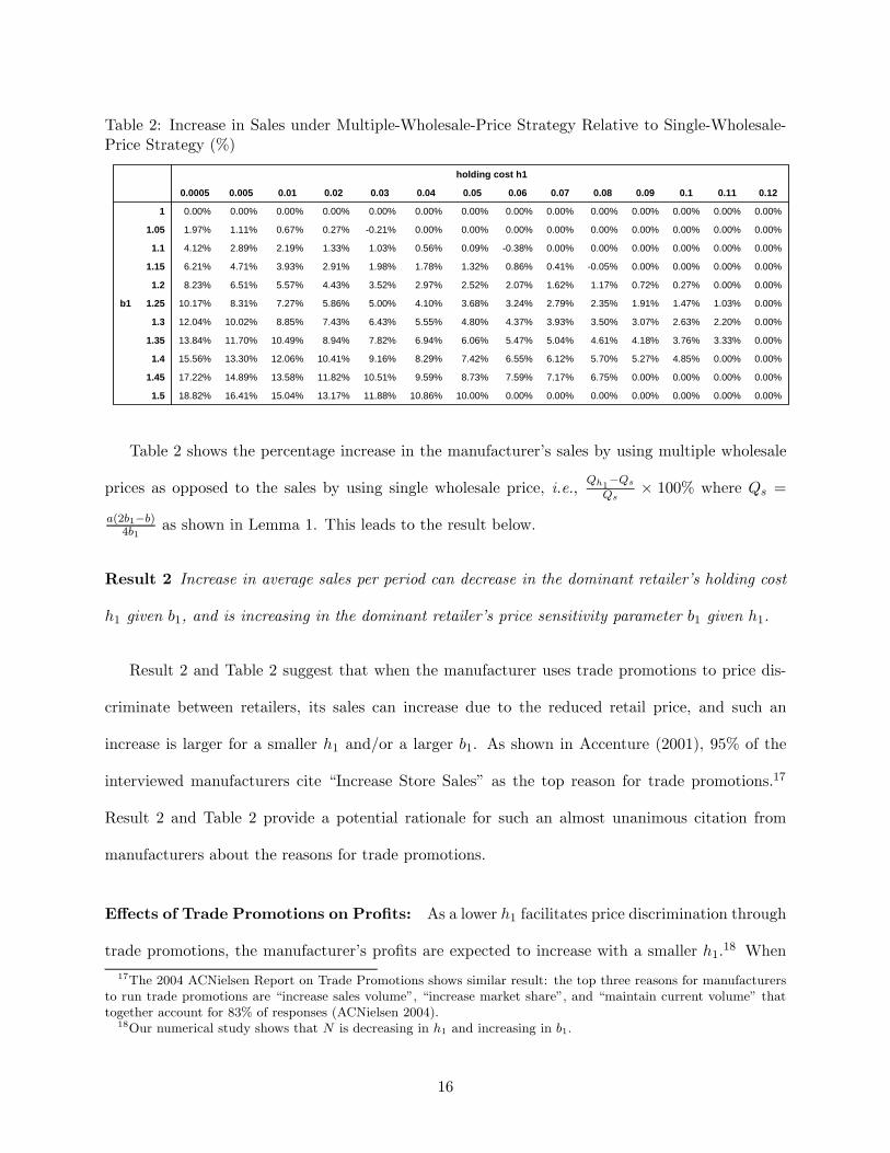
Table 2: Increase in Sales under Multiple-Wholesale-Price Strategy Relative to Single-Wholesale-Price Strategy (%)

0.00%0.00%0.00%0.00%0.00%0.00%0.00%10.00%10.86%11.88%13.17%15.04%16.41%18.82%1.5

0.00%0.00%0.00%0.00%6.75%7.17%7.59%8.73%9.59%10.51%11.82%13.58%14.89%17.22%1.45

0.00%0.00%4.85%5.27%5.70%6.12%6.55%7.42%8.29%9.16%10.41%12.06%13.30%15.56%1.4

0.00%3.33%3.76%4.18%4.61%5.04%5.47%6.06%6.94%7.82%8.94%10.49%11.70%13.84%1.35

0.00%2.20%2.63%3.07%3.50%3.93%4.37%4.80%5.55%6.43%7.43%8.85%10.02%12.04%1.3

0.00%1.03%1.47%1.91%2.35%2.79%3.24%3.68%4.10%5.00%5.86%7.27%8.31%10.17%1.25b1

0.00%0.00%0.27%0.72%1.17%1.62%2.07%2.52%2.97%3.52%4.43%5.57%6.51%8.23%1.2

0.00%0.00%0.00%0.00%-0.05%0.41%0.86%1.32%1.78%1.98%2.91%3.93%4.71%6.21%1.15

0.00%0.00%0.00%0.00%0.00%0.00%-0.38%0.09%0.56%1.03%1.33%2.19%2.89%4.12%1.1

0.00%0.00%0.00%0.00%0.00%0.00%0.00%0.00%0.00%-0.21%0.27%0.67%1.11%1.97%1.05

0.00%0.00%0.00%0.00%0.00%0.00%0.00%0.00%0.00%0.00%0.00%0.00%0.00%0.00%1

0.120.110.10.090.080.070.060.050.040.030.020.010.0050.0005

holding cost h1

Table 2 shows the percentage increase in the manufacturer's sales by using multiple wholesale

prices as opposed to the sales by using single wholesale price, i.e.,Qh1¡QsQs

£ 100% where Qs =

a(2b1¡b)4b1

as shown in Lemma 1. This leads to the result below.

Result 2 Increase in average sales per period can decrease in the dominant retailer's holding cost

h1 given b1, and is increasing in the dominant retailer's price sensitivity parameter b1 given h1.

Result 2 and Table 2 suggest that when the manufacturer uses trade promotions to price dis-

criminate between retailers, its sales can increase due to the reduced retail price, and such an

increase is larger for a smaller h1 and/or a larger b1. As shown in Accenture (2001), 95% of the

interviewed manufacturers cite \Increase Store Sales" as the top reason for trade promotions.17

Result 2 and Table 2 provide a potential rationale for such an almost unanimous citation from

manufacturers about the reasons for trade promotions.

E®ects of Trade Promotions on Pro¯ts: As a lower h1 facilitates price discrimination through

trade promotions, the manufacturer's pro¯ts are expected to increase with a smaller h1.18 When

17The 2004 ACNielsen Report on Trade Promotions shows similar result: the top three reasons for manufacturersto run trade promotions are \increase sales volume", \increase market share", and \maintain current volume" thattogether account for 83% of responses (ACNielsen 2004).18Our numerical study shows that N is decreasing in h1 and increasing in b1.

16

Table 3: Increase in The Manufacturer's Pro¯t under Multiple-Wholesale-Price Strategy Relativeto Single-Wholesale-Price Strategy (%)

0.00%0.00%0.00%0.00%0.00%0.00%0.00%0.06%0.47%0.92%1.54%2.44%3.14%4.38%1.5

0.00%0.00%0.00%0.00%0.01%0.27%0.55%0.90%1.38%1.90%2.63%3.66%4.45%5.86%1.45

0.00%0.00%0.02%0.31%0.61%0.91%1.22%1.63%2.19%2.77%3.61%4.76%5.64%7.23%1.4

0.00%0.07%0.40%0.73%1.07%1.42%1.78%2.18%2.83%3.51%4.43%5.70%6.68%8.45%1.35

0.00%0.21%0.58%0.97%1.36%1.76%2.16%2.57%3.26%4.04%5.02%6.41%7.49%9.43%1.3

0.00%0.06%0.50%0.94%1.39%1.85%2.31%2.78%3.39%4.28%5.30%6.81%7.97%10.07%1.25b1

0.00%0.00%0.05%0.56%1.08%1.60%2.13%2.67%3.21%4.11%5.17%6.77%7.99%10.21%1.2

0.00%0.00%0.00%0.00%0.27%0.87%1.48%2.10%2.72%3.34%4.56%6.11%7.36%9.63%1.15

0.00%0.00%0.00%0.00%0.00%0.00%0.16%0.87%1.59%2.31%3.14%4.63%5.82%8.00%1.1

0.00%0.00%0.00%0.00%0.00%0.00%0.00%0.00%0.00%0.35%1.20%2.18%3.09%4.87%1.05

0.00%0.00%0.00%0.00%0.00%0.00%0.00%0.00%0.00%0.00%0.00%0.00%0.00%0.00%1

0.120.110.10.090.080.070.060.050.040.030.020.010.0050.0005

holding cost h1

the dominant retailer has a larger demand share (a smaller b1), the pro¯tability of trade promotions

for the manufacturer is decreasing, as there is less surplus the manufacturer could take from the

competitive fringe through price discrimination. Table 3 shows the percentage increase in the

manufacturer's pro¯t by using multiple wholesale prices as opposed to a single wholesale price, i.e.,

¦h1¡¦s¦s

£ 100% where ¦s =a2(2b1¡b)2

8bb21as shown in Lemma 1. This leads to the result below.

Result 3 The increased pro¯ts from trade promotions as opposed to a single wholesale price for

the manufacturer are decreasing in the dominant retailer's holding cost h1, and has an inverted-U

relationship with the dominant retailer's price sensitivity parameter b1.

Result 3 provides a potential rationale for the vocal complaints in recent years by the manufac-

turers regarding the e®ectiveness of trade promotions. As dominant retailers such as chain stores

and warehouse clubs become larger (small b1), the bene¯ts of trade promotions to the manufacturer

decrease. It is such a change that prompts some manufacturers to re-evaluate the e®ectiveness of

their trade promotions. From this perspective, it is easy to see why practitioners recognize that

\success (of trade promotions) will be elusive unless independents are involved" and as far as the

e®ectiveness of trade promotions is concerned, manufacturers \need a strong, viable independent

sector" (Progressive Grocer Annual Report 2000, page 30).

17

We can also examine how retailers' pro¯tability is a®ected by the same parameters h1 and b1.

We summarize our results below.

Result 4 The bene¯ts from trade promotions for the dominant retailer can decrease in its holding

cost h1 and have an inverted-U relationship with b1. The competitive fringe retailers can become

either worse o® or better o® due to trade promotions. Their gain from trade promotions can increase

with h1 and can have a U-shaped relationship with b1.

Intuitively, as the holding cost h1 is a direct cost to the dominant retailer, a higher h1 will reduce

the dominant retailer's pro¯t. Our analysis shows that the increase in the dominant retailer's pro¯ts

has the highest value for the intermediate values of b1 (Figure 6 in Technical Appendix TB veri¯es

this result). The intuition for this is as follows. The dominant retailer's pro¯ts are a®ected by two

factors. One is the average pro¯t from each unit sold, and the other is the total number of units

sold. When b1 is large (close to3b2 ), the manufacturer o®ers a higher promotional depth relative to

the single-wholesale-price strategy (see Table 4) and the increase in the dominant retailer's average

pro¯t from each sale as opposed to the single-wholesale-price strategy gets higher. However, for

any p, its demand share is small for a large b1. The e®ect of a small demand share dominates the

e®ect of a high average pro¯t from each sale and, therefore, the dominant retailer's pro¯t is low

for a large b1. When b1 is small (close to b), the dominant retailer has a large portion of demand,

but the average pro¯t from each sale is small, as the manufacturer o®ers a higher w1. Thus, the

dominant retailer's pro¯ts will again be small. Therefore, the dominant retailer's pro¯t is ¯rst

increasing, and then decreasing with b1.

The numerical study also suggests that the pricing cycle will be shorter (N is smaller) for a

higher h1. As the ¯rst period within a pricing cycle is the only period during which the retailers in

the competitive fringe can make a pro¯t, they will have higher average pro¯ts with shorter pricing

cycles, implying that the competitive fringe's pro¯t increases in h1.

18

Table 4: Promotional Depth under Multiple-Wholesale-Price Strategy Relative to Single-Wholesale-Price Strategy (%)

0.00%0.00%0.00%0.00%0.00%0.00%0.00%17.50%16.86%18.63%19.17%18.79%19.41%19.83%1.5

0.00%0.00%0.00%0.00%12.86%12.51%12.17%16.36%15.70%17.38%16.40%17.40%17.94%18.25%1.45

0.00%0.00%12.63%12.27%11.92%11.57%11.21%15.20%14.51%13.82%15.07%15.95%16.42%16.57%1.4

0.00%12.06%11.70%11.33%10.97%10.60%10.24%14.00%13.29%12.58%13.71%14.46%14.48%14.83%1.35

0.00%11.13%10.76%10.38%10.00%9.62%9.24%8.87%12.05%11.31%12.30%12.92%12.86%13.01%1.3

0.00%10.20%9.80%9.41%9.02%8.63%8.24%7.84%10.77%10.00%10.86%10.61%10.81%11.09%1.25b1

0.00%0.00%8.84%8.44%8.03%7.62%7.21%6.80%6.39%8.66%7.86%8.99%9.08%9.09%1.2

0.00%0.00%0.00%0.00%7.03%6.60%6.17%5.75%5.32%7.29%6.45%6.58%6.92%7.01%1.15

0.00%0.00%0.00%0.00%0.00%0.00%5.12%4.67%4.23%3.78%5.00%4.94%4.73%4.81%1.1

0.00%0.00%0.00%0.00%0.00%0.00%0.00%0.00%0.00%2.65%2.18%2.58%2.54%2.50%1.05

0.00%0.00%0.00%0.00%0.00%0.00%0.00%0.00%0.00%0.00%0.00%0.00%0.00%0.00%1

0.120.110.10.090.080.070.060.050.040.030.020.010.0050.0005

holding cost h1

The competitive fringe gets the lowest pro¯t for intermediate values of b1 and more pro¯ts for

smaller and larger b1's as expected. Also note that for a large b1 and a large h1, the competitive

fringe could become better o® due to trade promotions. For a given b1, it is optimal for the

manufacturer to choose a shorter pricing cycle when h1 goes up. Thus, the promotional period

1, when the competitive fringe can get positive surplus, will occur more frequently as h1 becomes

larger and the competitive fringe becomes better o® as a result. For a given h1, the manufacturer

will o®er a lower w1 but will choose a longer pricing cycle when b1 becomes larger. When b1 is

very large, the positive e®ect of a lower w1 on the competitive fringe's pro¯ts will dominate the

negative e®ect of a longer pricing cycle and the competitive fringe becomes better o®. Therefore,

the competitive fringe's pro¯t is ¯rst decreasing, and then increasing in b1.

E®ects of Trade Promotions on Social Welfare: Many researchers have argued that trade

promotions are harmful to a channel because of increased inventory holding costs. Although our

model also suggests that trade promotions increase inventory holding costs, we ¯nd that trade

promotions can potentially bene¯t the system as a whole by enabling the manufacturer to price

discriminate between retailers. We state this result formally below (Figure 7 in Technical Appendix

TB veri¯es this result).

19

Result 5 Trade promotions can increase social welfare. The increase in social welfare is smaller

when the dominant retailer's holding cost h1 is larger or b1 is smaller (or the dominant retailer is

more dominant).

The source of the welfare improvement comes from the fact that price discrimination can allevi-

ate the problem of double marginalization in the channel, to the bene¯t of not only the manufacturer

and the retailers, but also the consumers. Trade promotions induce the dominant retailer to choose

a low retail price. Although the retail price goes up by h12 per period because of the presence

of the holding cost h1, the retail prices in most periods will be lower than the benchmark retail

price ps =a(2b1+b)4bb1

, the retail price that the dominant retailer would set if the manufacturer were to

charge all retailers the same time-invariant wholesale price ws =a(2b1¡b)2bb1

. Interestingly, competitive

fringe may even bene¯t from trade promotions as shown above. This is because the channel pro¯t

increases as the double marginalization problem is lessened and all channel members, including

the competitive fringe, can bene¯t from increased channel sales. Even when the competitive fringe

becomes worse-o® due to price discrimination, the total social welfare can still increase because

of the lower retail price set by dominant retailer. Consequently, trade promotions can improve

channel e±ciency and increase social welfare.

Overall, what emerges from Proposition 1 and Results 1-5 is a di®erent perspective on trade

promotions. Manufacturers embrace trade promotions because the practice allows them to im-

plement price discrimination in a distribution channel. In light of this perspective, it is rather

understandable that when manufacturers run trade promotions, they allow forward buying, but

disallow diversion. Our model can also explain why retailers do not all endorse this practice.

The dominant retailer favors such a practice as it stands to bene¯t from trade promotions due to

its low inventory holding costs. The competitive fringe could oppose such a practice, as it may

become worse o® because of the e®ective price discrimination that trade promotions achieve. How-

ever, this does not mean that such a practice is harmful because social welfare can increase with

this practice. Finally, manufacturers may have incentives to abandon this practice, as the retail

20

consolidation continues.19

5. Extensions

Our basic model leaves three important questions unanswered so far.

1. Does price-discrimination necessarily require multiple wholesale prices, as suggested by the

solution to the optimization problem (3.3)? If it does, such a theory would be rather counter-

factual, as in practice, we often observe manufacturers alternating between two wholesale

prices in a given period of time: the regular and discounted wholesale prices.

2. Does a price discrimination explanation of trade promotions also hold in the situations where

the competitive fringe has ¯nite (as oppose to in¯nite) inventory holding costs?

3. Does the price discrimination explanation of trade promotions depend on the assumption

of dominant retailer channel (i.e., only the dominant retailer has pricing power)? In other

words, if the competitive fringe independently and competitively sets its retail price, would

the manufacturer's incentives to use trade promotions to price discriminate go away?

5.1 Comparing 2-Price Model with the Full Model

In our basic model, as the optimal solution, the manufacturer's wholesale price increases every

period, after the initial dip, over the rest of the pricing cycle. This feature of our solution is not

necessary as two price points are su±cient for price discrimination to occur. In fact, there are three

ways to reconcile our optimal solution with the frequently observed trade promotion practice of

two price points. First, the parameters may be such that the optimal solution calls for a regular

wholesale price and a discounted price. In other words, there is a possibility that a 2-price solution

19This may well explain why the portion of trade promotion budgets allocated to o®-invoice allowances has decreasedfrom about 90 percent in mid-1990s to about 35 percent in recent years (Cannondale Associates 2003), but chainretailers, as they become more dominant through consolidation, prefer o®-invoice trade promotions to performance-based promotions such as scan-backs. G¶omez, Rao, and McLaughlin (2005) ¯nd that retailers with larger shareof private label, larger annual sales, and stronger brand positioning do demand more trade promotion funds too®-invoices.

21

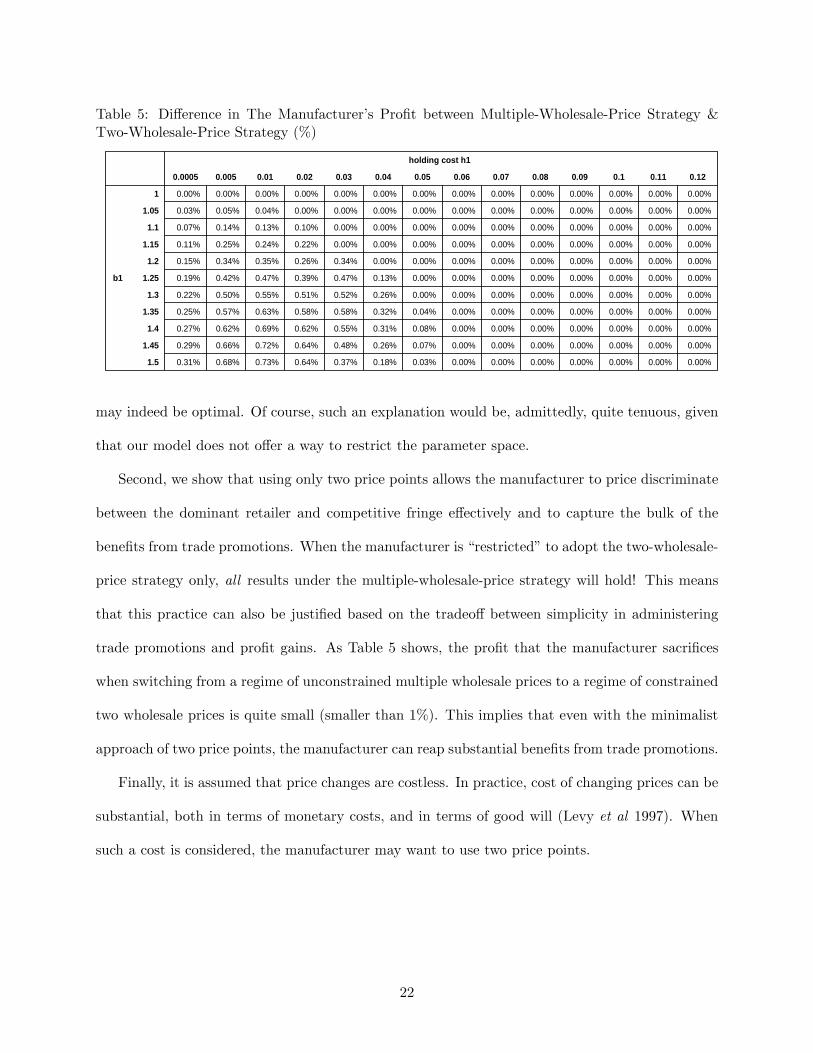
Table 5: Di®erence in The Manufacturer's Pro¯t between Multiple-Wholesale-Price Strategy &Two-Wholesale-Price Strategy (%)

0.00%0.00%0.00%0.00%0.00%0.00%0.00%0.03%0.18%0.37%0.64%0.73%0.68%0.31%1.5

0.00%0.00%0.00%0.00%0.00%0.00%0.00%0.07%0.26%0.48%0.64%0.72%0.66%0.29%1.45

0.00%0.00%0.00%0.00%0.00%0.00%0.00%0.08%0.31%0.55%0.62%0.69%0.62%0.27%1.4

0.00%0.00%0.00%0.00%0.00%0.00%0.00%0.04%0.32%0.58%0.58%0.63%0.57%0.25%1.35

0.00%0.00%0.00%0.00%0.00%0.00%0.00%0.00%0.26%0.52%0.51%0.55%0.50%0.22%1.3

0.00%0.00%0.00%0.00%0.00%0.00%0.00%0.00%0.13%0.47%0.39%0.47%0.42%0.19%1.25b1

0.00%0.00%0.00%0.00%0.00%0.00%0.00%0.00%0.00%0.34%0.26%0.35%0.34%0.15%1.2

0.00%0.00%0.00%0.00%0.00%0.00%0.00%0.00%0.00%0.00%0.22%0.24%0.25%0.11%1.15

0.00%0.00%0.00%0.00%0.00%0.00%0.00%0.00%0.00%0.00%0.10%0.13%0.14%0.07%1.1

0.00%0.00%0.00%0.00%0.00%0.00%0.00%0.00%0.00%0.00%0.00%0.04%0.05%0.03%1.05

0.00%0.00%0.00%0.00%0.00%0.00%0.00%0.00%0.00%0.00%0.00%0.00%0.00%0.00%1

0.120.110.10.090.080.070.060.050.040.030.020.010.0050.0005

holding cost h1

may indeed be optimal. Of course, such an explanation would be, admittedly, quite tenuous, given

that our model does not o®er a way to restrict the parameter space.

Second, we show that using only two price points allows the manufacturer to price discriminate

between the dominant retailer and competitive fringe e®ectively and to capture the bulk of the

bene¯ts from trade promotions. When the manufacturer is \restricted" to adopt the two-wholesale-

price strategy only, all results under the multiple-wholesale-price strategy will hold! This means

that this practice can also be justi¯ed based on the tradeo® between simplicity in administering

trade promotions and pro¯t gains. As Table 5 shows, the pro¯t that the manufacturer sacri¯ces

when switching from a regime of unconstrained multiple wholesale prices to a regime of constrained

two wholesale prices is quite small (smaller than 1%). This implies that even with the minimalist

approach of two price points, the manufacturer can reap substantial bene¯ts from trade promotions.

Finally, it is assumed that price changes are costless. In practice, cost of changing prices can be

substantial, both in terms of monetary costs, and in terms of good will (Levy et al 1997). When

such a cost is considered, the manufacturer may want to use two price points.

22

5.2 Finite Inventory Holding Costs for Both Retailers

If the competitive fringe has a ¯nite (as oppose to in¯nite in the basic model) unit inventory

holding cost but such cost is still higher than the dominant retailer's, i.e., 0 < h1 < h2 < 1,

the manufacturer can still use trade promotions to price discriminate. The proofs are in Technical

Appendix. The price discrimination comes about because of the extent to which di®erent retailers

can take advantage of trade promotions due to di®erences in holding costs.

5.3 Generalizing from the Dominant Retailer Model

Consider, for instance, an alternative demand model given by

Q1 = a1 ¡ b1p1 + c1p2

Q2 = a2 ¡ b2p2 + c2p1

where pi is the price for retailer i (Sayman et al 2002). In Technical Appendix TA, we show

that in this model the manufacturer can price discriminate between retailers through trade pro-

motions, even if both retailers independently and simultaneously make pricing decisions, as long

as minfb1; b2g > maxfc1; c2g. In other words, as long as the competing retailers exhibit di®erent

price sensitivities with regard to the wholesale price, and the higher price-sensitivity retailer has a

lower inventory holding cost, the manufacturer can bene¯t from price discrimination through trade

promotions.

6. Conclusion and Discussion

Many researchers have argued that trade promotions are harmful to manufacturers and to the

distribution channel because of the added inventory-holding costs. Using a dominant retailer model,

we show that trade promotions can bene¯t manufacturers and the channel precisely because of

the added inventory cost: these costs provide the manufacturers with an opportunity to price

discriminate between a dominant retailer and the competitive fringe. We show that the price

23

discriminating function of trade promotions is not speci¯c to the dominant retailer model and

works for other competitive models also.

What this analysis implies is that manufacturers may want to proceed cautiously to \rein

in" the practice of trade promotions. At the minimum, they need to weigh the bene¯t of price-

discrimination against any possible increase in the inventory and production costs in making such

decisions.

The price discrimination perspective also sheds some new light on the practice of trade pro-

motions. At a more general level, our analysis explains a few otherwise puzzling sets of practices

associated with trade promotions: manufacturers do not seem to complain about the e®ectiveness

of trade promotions or want to take the initiative of abandoning the practice (or when they do,

they su®er); manufacturers allow forward buying but not diversion; power retailers urge for trade

promotions but small and independent retailers frequently condemn the practice as unfair. Our

analysis shows that price discrimination implemented through trade promotions could favor the

manufacturer and the dominant retailer at the expense of the competitive fringe, and e®ective

price discrimination can be implemented if there is forward buying but no diverting on the part of

the dominant retailer.

Our analysis also shows that price discrimination induced through trade promotions can be

welfare-enhancing as it alleviates the problem of double-marginalization in a distribution channel.

We also show that trade promotions can increase social welfare, as the di®erence between retailers'

holding costs is su±ciently large or the dominant retailer's market share is su±ciently small (b1 is

large). Surprisingly, our analysis also ¯nds that trade promotions may also bene¯t the competitive

fringe under some conditions. The bene¯ts to the competitive fringe come during promotional

periods, in which all retailers enjoy the low wholesale price. Thus, when the dominant retailer has

a high holding cost h1 and a low market share (large b1), the manufacturer will promote frequently

with a high promotion depth to the bene¯t of the competitive fringe.

Our analysis suggests that one is more likely to observe trade promotions in industries or

24

product categories where inventory holding cost is su±ciently small, or power retailers are not too

dominant. These are testable predictions.

One could argue that trade promotions as a price discrimination mechanism are potentially

more e®ective and robust than other pricing mechanisms such as quantity discounts or a menu

of two part tari®s (Kuksov and Pazgal 2007). For instance, when a manufacturer uses quantity

discounts to price discriminate against small retailers, the small retailers may be able to get together

and pool their purchases to avail themselves of a low wholesale price. They can act similarly under

a menu of two-part tari®s. However, with trade promotions, the competitive fringe retailers need

to invest in joint warehouse facilities to be able to take advantage of periodic price deals. Said

di®erently, as a price discrimination mechanism, trade promotions generate potentially less leakage

than other posted price mechanisms.

While we believe that our analysis has generated some interesting new insights, it is important

to point out the limitations of our model. In our model, we do not explicitly model product di®er-

entiation, although a downward sloping demand curve for the dominant retailer does suggest some

di®erentiation in its o®erings. If the retailers in the competitive fringe can o®er vertically di®er-

entiated products to customers, we suspect that the competitive fringe will have more power and

can be more pro¯table compared with the current model.20 We do not consider the manufacturer's

holding costs in the model. If the manufacturer has to hold inventory instead of transferring all

inventory to retailers and has lower inventory holding costs than retailers, will trade promotions

still bene¯t the channel? We suspect that trade promotions can still be bene¯cial as the motivation

for and the e®ects of, price discrimination in a channel do not go away because of a lower inventory

holding cost on the part of the manufacturer. We also assume that the manufacturer is selling a

single product through retailers. In multiple product setting, studies on how trade promotions on

one product a®ect the pro¯ts of other products may generate additional insights (Chen and Xie

2007). Finally, we assume that the manufacturer is a monopoly in supplying products to retailers

20We thank an anonymous reviewer for pointing out this issue.

25

(Liu and Zhang 2006). It is important for future research to investigate whether trade promotions

could still help manufacturers to price discriminate between retailers in a competitive context. We

suspect that they still could, as competition rarely negates any incentive for price discrimination.

26

References

Accenture. 2001. The daunting dilemma of trade promotion: Why most companies continue to

lose the battle - and how some are winning the war.

ACNielsen. 2004. Fourteenth annual survey of trade promotion practices.

Ailawadi, Kusum L., Paul Farris, Ervin Shames. 1999. Trade promotion: Essential to selling

through resellers. Sloan Management Rev. 41(1) 83-92.

Agrawal, Deepak. 1996. E®ect of brand loyalty on advertising and trade promotions: A game

theoretic analysis with empirical evidence. Marketing Sci. 15(1) 86-108.

Blattberg, Robert C., Gary D. Eppen, Joshua Lieberman. 1981. A theoretical and empirical

evaluation of price deals for consumer nondurables. J. Marketing 45(1) 116-129.

Bruce, Norris, Preyas S. Desai, Richard Staelin. 2005. The better they are, the more they give:

Trade promotions of consumer durables. J. Marketing Res. 42(1) 54-66.

Buzzell, Robert D., John A. Quelch, Walter J. Salmon. 1990. The costly bargain of trade

promotion. Harvard Bus. Rev. 68(2) 141-149.

Cannondale Associates. 2002,2003. Trade promotion spending & merchandising industry study.

Chen, Yuxin, Jinhong Xie. 2007. Cross-market network e®ect with asymmetric customer loyalty:

Implications for competitive advantage. Marketing Sci. 26(1) 52-66.

Drμeze, Xavier, David R. Bell. 2003. Creating win|win trade promotions: Theory and empirical

analysis of scan-back trade deals. Marketing Sci. 22(1) 16-39.

Dukes, Anthony J., Esther Gal-Or, Kannan Srinivasan. 2006. Channel bargaining with retailer

asymmetry. J. Marketing Res. 43(1) 84-97.

Geylani, Tansev, Anthony J. Dukes, Kannan Srinivasan. 2005. Strategic manufacturer response

to a dominant retailer. Marketing Sci. Forthcoming.

G¶omez, Miguel I., Vithala R. Rao, Edward W. McLaughlin. 2005. Empirical analysis of budget

and allocation of trade promotions in the US supermarket industry. Working Paper, Cornell

University, Ithaca, New York.

Jeuland, Abel P., Chakravarthi Narasimhan. 1985. Dealing { temporary price cuts { by seller as

a buyer discrimination mechanism. J. Bus. 58(3) 295-308.

Jeuland, Abel P., Steven M. Shugan. 1983. Managing channel pro¯ts. Marketing Sci. 2(3)

239-272.

27

Jewell, William S. 1963. Markov-renewal programming. II: In¯nite return models, example. Oper.

Res. 11(6) 949-971.

Kahn, Barbara E., Leigh McAlister. 1997. Grocery Revolution, Addison-Wesley.

Kuksov, Dmitri, Amit Pazgal. 2007. The e®ects of costs and competition on slotting allowances.

Marketing Sci. 26(2) 259-267.

Lal, Rajiv. 1990. Manufacturer trade deals and retail price promotions. J. Marketing Res. 27(4)

428-444.

Lal, Rajiv, John D. C. Little, J. Miguel Villas-Boas. 1996. A theory of forward buying, merchan-

dising, and trade deals. Marketing Sci. 15(1) 21-37.

Levy, Daniel, Mark Bergen, Shantanu Dutta, Robert Venable. 1997. The magnitude of menu

costs: Direct evidence from large U.S. supermarket chains. Quart. J. Econom. 112(3) 791-

825.

Liu, Yunchuan, Z John Zhang. 2006. The bene¯ts of personalized pricing in a channel. Marketing

Sci. 25(1) 97-105.

Progressive Grocer. 2002. Stando® at the shelf: Big chains are happier with their treatment than

small independents, but not that happy. 81(6).

Progressive Grocer Annual Report 1981, 2000, 2003.

Raju, Jagmohan S., Z. John Zhang. 2005. Channel coordination in the presence of a dominant

retailer. Marketing Sci. 24(2) 254-262.

Samuelson, Paul A., William Nordhaus. 1989. Economics, New York: McGraw-Hill, 13th ed.

Sayman, Serdar, Stephen J. Hoch, Jagmohan S. Raju. 2002. Positioning of store brands. Mar-

keting Sci. 21(4) 378{397.

Sellers, Patricia. 1992. The dumbest marketing ploy. Fortune, Oct 5th.

The McKinsey Quarterly. 2003. Value-driven shopping. Robert Frank, Elizabeth A. Mihas, and

Laxman Narasimhan, Number 3.

U.S. Distribution Journal. 1992. Relations at the crossroads. December 17th.

U.S. Distribution Journal. 1993a. Quarter of wholesaler's income tied to trade promo funds:

Study. April 15th.

U.S. Distribution Journal. 1993b. Wholesalers under the microscope: a study of the wholesale

industry. May 15th.

Zwiebach, Elliot. 1990. Fair distribution sought for trade promo funds. Supermarket News.

28

Appendices

A. Retailers' Incentives To Reduce Holding Costs

Assume 0 < h1 · h2 < 1. The manufacturer will o®er a wholesale price w1 in the ¯rst periodand wi in period i. Further, it will charge a w1 and choose a pricing cycle length N such that the

competitive fringe will not make \bridge-buying", otherwise the manufacturer will o®er a single

wholesale price ws, instead of o®ering a trade promotion with both retailers making bridge-buying.

Intuitively, the dominant retailer, who is making \bridge buying", will have a larger incentive to

reduce unit holding cost since the dominant retailer will reduce unit acquisition cost in each of the

N periods. The competitive fringe, who has a unit holding cost h2 > h1 and is making \forward

buying" for a shorter period than N, will have a smaller incentive since it will bene¯t from reduced

holding cost in less than N periods. We will formally prove this result below.

Dominant retailer's incentives

Given w1 and N , the dominant retailer will choose a retail price pi = a+b1w1+b1h1(i¡1)

2b1in period

i and its e®ective unit acquisition cost in period i will be equal to w1 + (i ¡ 1)h1, (i = 1; :::; N).

Therefore, the dominant retailer's pro¯t in period i is given by

¼id = [pi ¡ w1 ¡ (i¡ 1)h1](a¡ b1pi); (A.1)

and its total pro¯t in one pricing cycle is given by

¼Td =NXi=1

¼id =NXi=1

[pi ¡ w1 ¡ (i¡ 1)h1](a¡ b1pi) (A.2)

The dominant retailer's incentive to reduce holding cost h1 is therefore given by21

@¼Td@h1

=NXi=1

@¼id@h1

= ¡NXi=1

(i¡ 1)(a¡ b1pi) = ¡NXi=1

(i¡ 1)Qdi < 0 (A.3)

That is, the dominant retailer's pro¯t will be higher as its holding cost h1 goes down.

Competitive fringe's incentives

We have stated that the retailers in the competitive fringe are not making bridge-buying as the

dominant retailer is. Otherwise, trade promotions will not be pro¯table for the manufacturer. How-

ever, the competitive fringe's non-in¯nity unit holding cost h2 makes it probable for the competitive

fringe to make forward-buying in the promotional period. Let ¹x be the number of periods in which

the competitive fringe's e®ective unit acquisition cost in period i = 1; :::; ¹x is lower than the retail

21Here we use marginal analysis in studying retailers' incentives to reduce unit holding cost. That is, given w1, N ,and ¹x (for competitive fringe), the dominant retailer's (any competitive fringe retailer's) incentive of reducing unitholding cost h1 (h2) is analyzed here.

29

price pi, if the competitive fringe makes forward-buying in the ¯rst period at the wholesale price

w1. That is, w1+ (¹x¡ 1)h2 · p¹x and w1+ (¹x+1¡ 1)h2 > p¹x+1. Knowing the competitive fringe'se®ective acquisition cost, the manufacturer will not charge the retailers in competitive fringe a

wholesale price equal to pi in periods 1 to ¹x, but charge them the e®ective unit acquisition cost

w1+ (i¡ 1)h2 to make competitive fringe retailers indi®erent between making forward-buying andordering from the manufacturer in each period. Since the e®ective unit acquisition cost is not

lower than the promotional price w1, the manufacturer could have higher pro¯ts by charging them

the e®ective acquisition cost than announcing a wholesale price equal to the retail price in period

i = 1; :::; ¹x. Assume x makes the constraint equal

w1 + (x¡ 1)h2 = px = a+ b1w1 + b1h1(x¡ 1)2b1

; (A.4)

and we get x = 1 + a¡b1w1b1(2h2¡h1) . Therefore we have,

¹x = int[x] = int[1 +a¡ b1w1

b1(2h2 ¡ h1) ] andx¡ 1 < ¹x · x (A.5)

Assume there are C identical retailers in the competitive fringe, each of whom has a demand

proportion of 1CQci =

1C (b1 ¡ b)pi in period i = 1; :::; N . Any retailer's e®ective unit acquisition

cost of each item sold in period i · ¹x equals ci2 = w1 + (i¡ 1)h2, and the retailer's pro¯t in periodi is given by

¹¼ic = [pi ¡ w1 ¡ (i¡ 1)h2]£ b1 ¡ b

Cpi (A.6)

The retailer's pro¯ts from period ¹x+1 to period N are zero because the manufacturer will take all

surplus from the competitive fringe by charging a wholesale price slightly lower than the market

price. So the total pro¯t within a pricing cycle for any retailer in competitive fringe is given by

¹¼Tc =¹xXi=1

¹¼ic =¹xXi=1

[pi ¡w1 ¡ (i¡ 1)h2]£ b1 ¡ bC

pi (A.7)

The incentive for any retailer in the competitive fringe to reduce holding cost h2 is given by

@¹¼Tc@h2

=¹xXi=1

@¹¼ic@h2

= ¡¹xXi=1

(i¡ 1)b1 ¡ bC

pi = ¡¹xXi=1

(i¡ 1) 1CQci < 0 (A.8)

That is, the competitive fringe's pro¯t will be higher as the holding cost h2 goes down.

Since ¹x < N , equations (A.3) and (A.8) show that the dominant retailer has more incentives

than any competitive fringe to reduce holding costs if the dominant retailer's demand (Qdi) is not

smaller than the demand of any retailer in the competitive fringe ( 1CQci) in periods i = 1; :::; ¹x, orPNi=1(i¡ 1)(a¡ b1pi) >

P¹xi=1(i¡ 1) b1¡bC pi for Qdi ¸ Qci

C . Q.E.D.

30

B. Proof of Lemma 1. Conditional on wholesale price ws, the dominant retailer's pro¯t in any

period is given by,

¼d;s = (ps ¡ws)(a¡ b1ps): (B.1)

The F.O.C. of the pro¯t function determines the dominant retailer's optimal retail price, which is

given by

ps =a+ b1ws2b1

(B.2)

and retailers' demands are given by(Qd;s = a¡ b1ps = a¡b1ws

2

Qc;s = (b1 ¡ b)ps = (b1¡b)(a+b1ws)2b1

: (B.3)

The manufacturer chooses ws to maximize its pro¯t ¦s = ws(Qd;s+Qc;s). The optimal ws is given

by

ws =a(2b1 ¡ b)2bb1

: (B.4)

Given ws =a(2b1¡b)2bb1

, it is easy to derive other results in the lemma. Q.E.D.

Proof of Lemma 2. The way to prove Lemma 2 is to consider the dominant retailer's decisions

in an arbitrary period based on e®ective unit acquisition cost. The dominant retailer purchases

inventory in the ¯rst period at a wholesale price w1 and will be charged a unit holding cost h1 > 0

per period for inventory it carries from one period to the next. Thus the e®ective unit acquisition

cost of the units sold in period j = 1; :::; N is equal to w1 + (j ¡ 1)h1. Here w1 is the originalpurchase cost and (i¡1)h1 is the holding cost charged to each unit sold in period i. Therefore, thedominant retailer's pro¯t for period j is given by,

¼jd;h1 = [pj ¡w1 ¡ (j ¡ 1)h1](a¡ b1pj) (B.5)

and it will choose a retail price pj = a+b1w1+b1h1(j¡1)2b1

in period j. Both the dominant retailer and

the competitive fringe pay the promotional wholesale price w1 in the ¯rst period. From the second

period on, the manufacturer will charge the competitive fringe a wholesale price equal to the retail

price to get all surplus from the competitive fringe since the competitive fringe takes the retail price

pj as given in any period j. That is, wj = pj for j = 2; :::; N . The manufacturer's average pro¯t

per period in a pricing cycle is given below.

¦h1 =1

N[w1

NXi=1

(a¡ b1pi) +w1(b1 ¡ b)p1 +NXj=2

wj(b1 ¡ b)pj ]; (B.6)

wherePNi=1(a ¡ b1pi) is the dominant retailer's total ordering quantity, pi = a+b1w1+b1h1(i¡1)

2b1is

the retail price in period i, and wj = pj is the wholesale price in period j = 2; :::; N . Since ¦h1 is

strictly concave in w1, F.O.C. solves w1 as follows.

w1 =N [4ab1 ¡ 2ab¡ bb1h1(N ¡ 1)]2b1[b(N + 1) + b1(N ¡ 1)] (B.7)

31

Other results in Lemma 2 can then be easily derived. Q.E.D.

Proof of Proposition 1. If 0 · h1 < h2 =1, the manufacturer will o®er wholesale prices w1 andwi (i = 2; ::;N) as in equation (3.1). For items sold in the promotional period, both the dominant

retailer and competitive fringe are having same unit acquisition cost w1. For items sold in period

i = 2; :::;N , the unit acquisition cost for the dominant retailer is equal to w1 + h1(i ¡ 1) and thecost for the competitive fringe is equal to the wholesale price in that period wi =

a+b1w1+b1h1(i¡1)2b1

.

We have wi ¡ [w1 + h1(i ¡ 1)] = a¡b1[w1+h1(i¡1)]2b1

= a¡b1pib1

> 0. Therefore, the competitive fringe

is paying a higher average unit acquisition cost in a pricing cycle than the dominant retailer. If

0 · h1 < h2 < 1, the same logic still applies as long as the optimal pricing cycle length N ¸ 2.The only di®erence is that it is possible that the retailers in the competitive fringe would also like

to carry some inventory from one period to the next, but they will carry items for fewer periods

than the dominant retailer because of their higher inventory holding cost. If they are carrying

items for the same periods as the dominant retailer, trade promotions will not be worthy for the

manufacturer and the optimal N will be equal to 1, i.e., no trade promotions are o®ered. Q.E.D.

C. Credibility of Manufacturer's Announcement of N and wi (i = 1; :::; N)

In this section we will show that the manufacturer's announcement of both the length of pricing

cycle N and the wholesale price wi for each period i within a pricing cycle consisting of N periods

(i = 1; :::; N) are credible. That is, given the announced N and wi (i = 1; :::;N) determined as

in Lemma 2, the manufacturer will not have incentives to deviate from them. The intuition is as

follows. Given the preannounced optimal N, the manufacturer will not have incentive to extend

N to any ~N > N . The reason for the manufacturer to run trade promotions is because trade

promotions will provide a higher average pro¯t per pricing cycle for the manufacturer than a time

invariant wholesale price. If a manufacturer deviate from N to ~N > N and charge the optimal time

invariant wholesale price ws as shown in Lemma 1 for periods N +1; :::; ~N (the dominant retailer's

inventory ordered in period 1 will be depleted in period N), the manufacturer will get a lower

average pro¯t per period for periods N + 1; :::; ~N . Given the preannounced N , the manufacturer

will have no incentive to deviate to any ¹N < N either. In a pricing cycle, the manufacturer gets a

much lower pro¯t from units sold in period 1 than the average pro¯t per period in the pricing cycle

since the wholesale price w1 is low and available to both the dominant retailer and competitive

fringe. In each period i (i = 2; :::; N), however, the manufacturer will get a higher than average

pro¯t from units sold in the period. The higher than average pro¯t comes from the manufacturer's

complete gain of competitive fringe's surplus by charging a wholesale price equal to retail price in

each period. If the manufacturer deviates to any ¹N < N , it will get a lower average pro¯t per

period for each pricing cycle since the manufacturer is cutting o® the high pro¯t periods ¹N+1; :::; N

while the dominant retailer will bring unsold units (due to the truncation of the pricing cycle) to

32

the next pricing cycle. The manufacturer will thus have no incentive to either extend or shorten

a pricing cycle from N to any ~>N or ¹N < N . In any period i = 2; :::;N , the manufacturer will

have no incentive to deviate from the preannounced wi either. Since wi = pi for i = 2; :::; N , the

manufacturer will not increase the wholesale price since such an increase will let the manufacturer

lose the pro¯t from competitive fringe by making the wholesale price for the competitive fringe

higher than the retail price. The manufacturer will also have no incentive to decrease wholesale

price. If the reduced wholesale price in any period i = 2; :::; N (denoted as ¹wi) is so low that

the dominant retailer ¯nds it pro¯table to make an order, it is equivalent to the case where the

manufacturer starts a new pricing cycle (equivalently, chooses an ¹N < N), which is not optimal for

the manufacturer as shown above. If the reduced wholesale price is not low enough to induce the

dominant retailer to order in period i = 2; :::; N , the manufacturer will lose a margin of wi ¡ ¹wi

from competitive fringe, which is also not optimal. Either way, the manufacturer will not get a

higher pro¯t by deviate from the preannounced wi. Thus, the manufacturer will not deviate from

the preannounced N and wi (i = 1; :::; N).

Now we will proceed the proof in the following steps. First, we will show that the manufacturer

will not have incentives to deviate from the optimal N . Second, we will show that the manufacturer

will not have incentives to deviate from wholesale price wi for each period i within a pricing

cycle consisting of N periods (i = 1; :::; N), given the dominant retailer's order in the ¯rst period

Q1d =PNi=1Qdi =

N4 [2(a¡ b1w1)¡ b1h1(N ¡ 1)].

No Deviation from N

Given both dominant retailer's and competitive fringe's decisions in Lemma 2, the manufacturer will

not increase the length of pricing cycle from the optimal N to any ~N for N < ~N < 2N 22. Suppose

the manufacturer changes the length of pricing cycle from N to ~N after the dominant retailer

makes its order in the ¯rst period Q1d =N4 [2(a¡ b1w1)¡ b1h1(N ¡ 1)]. It is then optimal for the

manufacturer to set a wholesale price at ws =a(2b1¡b)2bb1

for each period j (j = N + 1; N + 2; :::; ~N)

and gets an average pro¯t per period of ¦s =a2(2b1¡b)2

8bb21for periods N + 1; N + 2; :::; ~N , if trade

promotions are not used between periods N + 1 and ~N 23. Since the reason for the manufacturer

to provide trade promotions is because trade promotions will provide a higher average pro¯t to

the manufacturer than a common time-invariant wholesale price to retailers, it is not optimal for

the manufacturer to deviate from N to any ~N > N . Now lets show the manufacturer also has no

incentives to shorten N to any ¹N < N . In order to prove so, we need the following lemma, which

shows that the manufacturer's pro¯t from sales in period N is the smallest among periods 2; :::; N .

22If ~N ¸ 2N , then the focal periods we focus on will be from period iN ¢N to period ~N where iN = int[~NN]. We

will then get similar insights as in the case where N < ~N < 2N .23An alternative way is for the manufacturer to use trade promotions to price discriminate between retailers between

periods N + 1 and ~N , but such a shorter pricing cycle will be suboptimal compared with the optimal pricing cyclewith a length of N since the optimal N is determined such that it pro¯t-dominates any other length of pricing cycle[please see Problem (3.3)].

33

Lemma 3 In a pricing cycle, the manufacturer's pro¯t from sales in a period is the minimum in

period j = minfN; bb1w1¡(b1¡b)(a¡b1h1)b1h1(b1¡b) g among periods 2; :::; N .

Proof of Lemma 3. The sales in any period j = 2; :::;N consists of two parts - sales of the items

the dominant retailer orders in period 1 at a wholesale price w1 and carries to period j and sales of

the items the ¯rms in competitive fringe order from the manufacturer at a wholesale price wj and

sell in period j. The sales in period j is equal to Qj = a¡ bpj = 2ab1¡ab¡bb1w1¡bb1h1(j¡1)2b1

as shown

in Lemma 2. Manufacturer's pro¯t from the sales in period j = 2; :::; N is thus given by

¦jh1 = w1Qdj + wjQcj

=w1[a¡ b1w1 ¡ b1h1(j ¡ 1)]

2+(b1 ¡ b)[a+ b1w1 + b1h1(j ¡ 1)]2

4b21(C.1)

The derivatives of ¦jh1 with respect to j are given by8><>:d¦j

h1dj = h1[a(b1¡b)+b1h1(b1¡b)(N¡1)¡bb1w1]

2b1d2¦j

h1dj2

=h21(b1¡b)

2 > 0(C.2)

Since the twice derivative of ¦jh1 with respect to j is positive, ¦jh1is strictly convex in j. Therefore,

the manufacturer's pro¯t ¦jh1 from sales is the minimum in period j = minfN;bb1w1¡(b1¡b)(a¡b1h1)

b1h1(b1¡b) gamong periods 2; :::; N , where bb1w1¡(b1¡b)(a¡b1h1)

b1h1(b1¡b) is solved from the F.O.C. of ¦jh1 . Q.E.D.

When the manufacturer o®ers trade promotions in period 1, the promotional wholesale price

w1 is same for both the dominant retailer and competitive fringe and w1 is di®erent from the

optimal constant wholesale price ws. Thus, the manufacturer's pro¯t from sales in period 1 is

smaller than the average pro¯t under constant wholesale price ¦s =a2(2b1¡b)2

8bb21. Since the reason

for the manufacturer to o®er trade promotions in the current model is because of a higher average

pro¯t in a pricing cycle than ¦s, the manufacturer's pro¯t from items sold in period 1 is therefore

smaller than the average pro¯t in a pricing cycle. Starting from period 2, the manufacturer will

have to get a higher pro¯t from the items sold in each period than the average pro¯t in order to

\compensate" the pro¯t \loss" in period 1. The higher than average pro¯t in each period comes

from sales to competitive fringe at a wholesale price of wi = pi. Such a \compensation" process

continues until a period when the pro¯t from that period is no longer contributable to improving

the average pro¯t per period in a pricing cycle, i.e. the average pro¯t in that period is smaller than

the average pro¯t in a pricing cycle 24 25. Thus the manufacturer will have no incentive to \cut"

24Numerical study shows that within the wide parametric rangesd¦

jh1dj

is negative for j = N . That is, themanufacturer's average pro¯t in each period among periods 2; :::; N is decreasing in j for the studied parametricvalues.25The manufacturer's pro¯t from items sold in period i by both retailers instead of its pro¯t from items sold in

period i by competitive fringe only should be considered here. This is because if the manufacturer truncates a pricingcycle at period i then the items that could have been sold by the dominant retailer in period i will be carried over tothe \new" pricing cycle in an in¯nitely repeated game.

34

Table 6: Comparison of The Manufacturer's Pro¯t in Period minfN; bb1w1¡(b1¡b)(a¡b1h1)b1h1(b1¡b) g and Av-erage Pro¯t

0.00%0.00%0.00%0.00%0.00%0.00%0.00%0.55%0.79%0.27%0.11%0.33%0.11%0.02%1.5

0.00%0.00%0.00%0.00%1.66%1.83%2.02%0.60%0.91%0.23%0.74%0.32%0.08%0.01%1.45

0.00%0.00%1.61%1.81%2.01%2.23%2.45%0.57%0.96%1.39%0.76%0.28%0.02%0.01%1.4

0.00%1.53%1.76%2.00%2.25%2.51%2.78%0.45%0.93%1.45%0.71%0.20%0.22%0.01%1.35

0.00%1.44%1.73%2.02%2.33%2.64%2.95%3.28%0.79%1.41%0.59%0.06%0.12%0.00%1.3

0.00%1.10%1.45%1.81%2.18%2.55%2.92%3.30%0.48%1.22%0.34%0.57%0.35%0.03%1.25b1

0.00%0.00%0.83%1.26%1.70%2.15%2.59%3.05%3.50%0.82%1.73%0.29%0.14%0.04%1.2

0.00%0.00%0.00%0.00%0.76%1.30%1.83%2.38%2.92%0.12%1.20%0.89%0.31%0.03%1.15

0.00%0.00%0.00%0.00%0.00%0.00%0.42%1.08%1.74%2.39%0.26%0.19%0.41%0.04%1.1

0.00%0.00%0.00%0.00%0.00%0.00%0.00%0.00%0.00%0.42%1.23%0.27%0.20%0.03%1.05

0.00%0.00%0.00%0.00%0.00%0.00%0.00%0.00%0.00%0.00%0.00%0.00%0.00%0.00%1

0.120.110.10.090.080.070.060.050.040.030.020.010.0050.0005

holding cost h1

at any period i for 2 < i < N since such a cutting will let the manufacturer lose the high margin

in period i associated with the order from competitive fringe and, at the same time, orders from

the dominant retailer will not increase because any orders unsold due to the \cutting" will not be

absorbed by the dominant retailer but be carried over to and sold in the new pricing cycle. This

will generate a smaller average pro¯t per period in a pricing cycle.

Table 6 shows numerical that the manufacturer's pro¯t in period minfN; bb1w1¡(b1¡b)(a¡b1h1)b1h1(b1¡b) gis always larger than its average pro¯t per period in the pricing cycle when the manufacturer

chooses to o®er trade promotions to retailers. Therefore, the manufacturer has no incentive

to truncate any pricing cycle into a pricing cycle with a length of ¹N < N since the period

minfN; bb1w1¡(b1¡b)(a¡b1h1)b1h1(b1¡b) g with the lowest average pro¯t among periods 2; :::; N has a higher

than average pro¯t. That is, the announcement of optimal N is credible and self-enforcing - the

manufacturer will not deviate to any ~N > N or ¹N < N in any period i = 2; :::; N within a pricing

cycle.

No Deviation from wi

In this subsection, we will show that the manufacturer will not deviate from pre-announced whole-

sale price wi in any period within a pricing cycle.

With the announced sequence of wholesale prices wi (i = 1; :::; N), the manufacturer will charge

the lowest wholesale price in period 1 in order to induce the dominant retailer to make forward-

buying. From period 2 until period N, the manufacturer will charge a wholesale price equal to

retail price in each period in order to take full surplus from competitive fringe. In any period

i = 2; :::; N , the manufacturer will not increase the wholesale price wi to any larger price since such

an increase will make the wholesale price higher than the retail price and thus the manufacturer

will lose sales from competitive fringe. The margin with the dominant retailer, at the same time,

35

does not improve because there is no sales to the dominant retailer in any period except in period

1 in a pricing cycle.

The manufacturer will also have no incentive to lower the wholesale price wi in any period

i = 2; :::; N . Suppose the manufacturer sets a wholesale price ¹wi < wi in period i. One of the

following two consequences will happen. In the ¯rst consequence, the new wholesale price is not

low enough so the dominant retailer will keep selling inventory carried over from period 1, i.e.

¹wi ¸ w1 + h1(i ¡ 1). Such a decrease will then only decrease the manufacturer's pro¯t since themargin the manufacturer gets from orders from competitive fringe is smaller while sales do not

change at all. In the other consequence, the new wholesale price makes it more pro¯table for the

dominant retailer to order from the manufacturer in period i, i.e. ¹wi < w1 + h1(i ¡ 1). This isessentially same as the case where the manufacturer restarts a new pricing cycle. As shown above

that it is not optimal for the manufacturer to deviate from the pre-announced N to any ¹N < N ,

the manufacturer will not decrease wholesale price from wi to any ¹wi < w1 + h1(i ¡ 1) in periodi = 2; :::; N .

Therefore, the manufacturer's announcements of both the length of pricing cycle N and the

sequence of wholesale prices wi, i = 1; :::; N , are credible and self-enforcing. Q.E.D.

36