A Predictive Model of Patient Readmission Using Combined ICD-9 Codes as Engineered Features

Robert P. Yerex, Ph.D1 Zachary Terner2

UVA Medical Center Accountable Care Organization1 University of California, Santa Barbara2

Abstract

The timing of post-discharge care is a significant factor in reducing unplanned hospital readmission. Statistical learning techniques can be applied to the development of models that predict the likelihood of patient readmission during the critical 30 day post-discharge period. The accuracy of these models is dependent on the quantity and quality of data used for training and validation. For Medicare and Medicaid patients who are members of an Accountable Care Organization (ACO), the Centers for Medicare and Medicaid (CMS) provides detailed claims based data that can be used, if appropriately collated, and transformed. This involves the identification and creation of useful features, which when included in the model, increases its predictive strength. Creation of derived features (feature engineering) is a process in which a large number of base dimensions (n) are combined to create a smaller

features set , reducing the complexity of the model while retaining its inherent information value. The inpatient admission diagnoses, in the form of ICD-9 codes, are an example of high dimensionality attributes found in the CMS claims data. Patterns inherent in the combinations of these codes can be used to create an engineered feature. In this study, a taxonomy of patterns of patient diagnoses was developed that was then used as a feature within a random survival forest model that predicts the hazard function (where the hazard event is unplanned readmission) of an individual patient for the first 30 days post discharge. Over the ensuing 30 days after release from hospital, a patient’s likelihood of readmission can be dynamically estimated based on the remaining portion of the hazard curve. Inclusion of the multiple diagnoses feature increased model accuracy to the point where it could be effectively used as a tool for targeting post-discharge patient care.

, reducing the complexity of the model while retaining its inherent information value. The

Introduction

Reducing 30-day readmissions has become a national priority for medical personnel and government agencies. Jencks, Williams, and Coleman estimate that the cost to Medicare in 2004 of unplanned hospital readmission was $17.4 billion [1]. Thus, there have been numerous efforts to reduce readmissions, including a penalty and incentive program implemented by Centers for Medicare and Medicaid Services, or CMS [2]. Krumholz et al. examine hospital performance, as measured by 30-day readmission and mortality rates, for patients with a primary diagnosis of acute myocardial infarction (AMI) or heart failure (HF) in different parts of the country. The study concluded that 30-day rates differed among hospitals in different parts of the country, and that readmission rates in particularpresent a good opportunity for improvement [2]. Addressing this need, numerous studies have been conducted todevelop predictive models that identify discharged patients at high risk of readmission. In a comprehensive reviewof 30 studies which developed predictive models for hospital readmission, Kansagara et al. conclude that mostreadmission risk prediction models perform poorly, corroborating the need for improvement [3]. Considering 30-dayreadmission rates for general surgery patients, Kassin et al find that postoperative complications appear to drivesurgical readmissions [4]. In a broader study on heart failure patients, Amarsingham et al. use a variety of predictors,such as measures of social instability and socioeconomic status, as well as EMR data and data available uponadmission, to predict readmissions [5]. Additional studies into readmission targeted Veterans Affairs (VA) hospitalsspecifically: Kaboli et al. investigate associations between reducing length of stay for VA patients under the concernthat a shorter stay would lead to increased readmissions [6]; Glasgow, Vaughn-Sarrazin, and Kaboli focus on VA

n n*

patients who left against medical advice (AMA), finding that AMA patients had higher 30-day mortality and readmission rates than other discharged patients [7].

To identify discharged patients at high risk of readmission, several studies have developed risk indices. Most notably, van Walvaren et al. develop the LACE index, which uses length of stay (L), acuity of admission (A), comorbidities as calculated via Charlson score (C), and the number of ED visits in the previous six months (E) to quantify odds of readmission [8]. Gruneir et al. validate the LACE index, suggesting the tool can be used to identify candidate patients for post-discharge interventions [9]. Conversely, Cotter et al. apply LACE to a population of older patients, finding that the index was not very predictive in that population [10]. Further studies build upon LACE, including an extension by van Walvaren et al. known as LACE+ [11], and a risk score termed HOSPITAL by Donze which includes hemoglobin, sodium at discharge, and a few other predictors [12].

In this study, we similarly attempt to identify patients at high risk of readmission. Using predictors identified primarily from CMS claims as found in the Claim and Claim Line Feed (CCLF) files provided by the Centers for Medicare & Medicaid Services (CMS), to participating Accountable Care Organization (ACO) [13], in combination with location based socioeconomic predictors available freely online, we identify which patients are at highest risk of 30-day readmission. We employ a random survival forest technique (RSF) to generate accurate predictions and provide insight into which variables are most important. Additionally, we engineer several new features from combined ICD-9 codes in a patient's claim, showing that these claims contain information that can be used in prediction. The next sections detail; the types of data used, the feature engineering process, the modeling technique of random survival forest (RSF), as well as the results of applying the model to a large data set.

Data Sources

The Centers for Medicare and Medicaid Services, or CMS, established the Accountable Care Organization (ACO) model, where groups of health care providers could unite to form their own ACO. Providers within an ACO work together to coordinate care for the member Medicare beneficiaries. As a result of their collaboration, ACOs are eligible to receive a share of the savings that they generate for the Medicare program [14]. The University of Virginia Health System participates in the Well Virginia ACO, which serves over 20,000 Medicare beneficiaries [15]. The data used for development of the predictive models in this study included claims based information extracted from the Claim and Claim Line Feed (CCLF) files provided by the Centers for Medicare & Medicaid Services (CMS). Because they are transaction oriented, considerable data manipulation was required in order to transform the CCLF records into a set of event history records for each patient describing one or more spells of care that involved one or more episodes of inpatient hospital care. The final data set included 5,364 patients with a total of 10,167 inpatient care episodes1 encompassed within 9,461 care spells. The earliest inpatient event occurred on 2013-01-01 and the last on 2014-09-17.

In addition to the claims data, additional features in the model consist of a range of socioeconomic variables. Several studies indicate that socioeconomic status and the environments in which patients live can affect their readmission rates [16], [17], [18]. Therefore, to add additional socioeconomic data to the model, we downloaded data for the state of Virginia from the County Health Rankings website provided by the University of Wisconsin Population Health Institute [19]. These variables include demographic health data, such as the percentage of adults in each county who are obese, the percentage of adults who smoke, and the percentage of adults who are diabetic, as well as variables that relate to the level of care available in each county, such as the number of dentists and the number of primary care physicians in each county. With the patient’s address, it was also possible to determine the US census block in which they resided [20]. Using this information it was possible to extract information on a variety of socioeconomic factors [21]. Included in the model were factors related to median income, and level of education.

1 As defined here, an episode of inpatient care can be described as a contiguous period of time when a patient was treated in a specific location for a specified condition. A spell of care is a chain of related episodes in chronological order.

Model Development

As described earlier, the performance of the currently published models designed to predict 30 day readmission is poor, suggesting that there are relationships between factors attributable to the patients and their environment, the course of their treatment, the progression of their illness, and the likelihood they will be readmitted within 30 days of discharge, which are too complex to be captured with simpler predictive model algorithms targeting categorical outcomes. In many fields where predictive modeling is used, the desire for the most accurate prediction far outweighs the need for interpretability; this is not generally true in the medical field where there is a tension between prediction and interpretation. If a model is to be designed to predict patient readmission as accurately as possible, it should not be constrained by the requirement for interpretability. Kuhn and Johnson, among others have stated that in a medical setting, it would be unethical to adopt a model that is more easily interpreted at the sacrifice of accuracy. “As long as the model can be appropriately validated, it should not matter whether it is a black box or a simple interpretable model” [22].

Statistical Learning Technique for Survival Function Estimation

Time to patient readmission data is amenable to the application of survival modeling, a collection of statistical techniques that take into many of the issues inherent in dealing with time to event data including censoring and competing risks [23]. While a variety of algorithms are available for estimation of the survival and related hazard functions in the presence of covariates. However most of these methods rely on restrictive assumptions such as proportional hazards, and are typically parametric in nature, requiring assumption of first, second, and third moments of the generating functions associated with the underlying selected parametric density family. Depending on the assumed density function, nonlinear effects of variables must be handled through transformations or expansion to include specialized basis functions. When there are multiple, possibly interacting covariates present, they are difficult to identify, and typically involves the researcher examining all two-way and three-way interactions, possibly relying on subjective knowledge to narrow the search. Non-parametric methods exist for the estimation of the survival function [24], such as the Kaplan–Meier estimator [25]. The advantage of these methods is their ease of use, but they are most suitable for controlled cohort analysis.

Several methods within the area of statistical learning can be used for functional approximation. Cybenko’s theorem [26] proves that a type of neural network (ANN) which is equivalent to the superimposition of multiple sigmoidal functions, can be used as a near perfect approximator for arbitrary monotonic functions. Unfortunately, ANN methods do not easily take into account censoring as occurs in survival analysis. Random Forests (RF) Another well-known statistical learning method that can be thought of as universal function approximators [27]. RF is a subset of a more general class of ensemble learning2 based techniques that iterate over combinations of base or weak learners with the resulting learner (the ensemble of the iterated base learners) having greater predictive power . While RF is generally used for regression and classification, Ishwaran et al. [28] have extended the technique specifically for use in survival analysis and is known as Random Survival Forests (RSF). In RFS, the splitting criterion used in growing a tree explicitly invokes survival time and censoring information. The effectiveness of a particular split is measured via the difference in survival expectation for inclusion in each of the new nodes below the split.

Random Survival Forest

Random survival forest models have been used in a variety of health applications, including in studies on esophageal cancer [29], as well as studies on patients with systolic heart failure [30] and Fontan patients who undergo cardiopulmonary exercise testing [31]. RSF models have even been used outside of the health domain in a credit risk

2 Ensemble learning is the process by which multiple models, such as classifiers or experts, are strategically generated and combined to solve a particular computational intelligence problem. Ensemble learning is primarily used to improve the (classification, prediction, function approximation, etc.) performance of a model, or reduce the likelihood of an unfortunate selection of a poor one

management model for small medium enterprises [32]. However, while random forest techniques have been used in a 30-day readmission setting previously [33], random survival forest techniques had notbeen applied to a 30-day readmission problem. In this paper, we apply RSF models to the 30-day readmission setting, using the randomForestSRC package in R [34].

Model Development, Training and Testing

A Random Survival Forest (RSF) was developed using the techniques outlined by Ishwaran et al. [12]. The initial data was split into training and test sets of 7,095 and 2,366 respectively. The parameters that can be controlled when using the particular implementation of RSF [13] include; number of trees constructed (ntree), number of candidate features to try at each split (ntry), minimum number of cases in a terminal node (nodesize), the maximum depth of any tree (nodedepth), and the splitting rule (splitrule).

Features in the final model are of two forms; simple and derived (engineered). Simple features are directly related to attributes in the data set3 . Derived features are generated through, sometimes complex, combinations and transformations of attributes in the data set. Features fell into several broad categories; Demographic: Age, gender and race.

Socioeconomic: As described earlier, these included US Census based measures of median income and education as well as county based health statistics.

Access to Care: With the location information, it was also possible to create several features used as surrogates for ease of access to care such as; distance to PCP, distance to admitting facility. For spells covering multiple claims and multiple facilities, the distance to the initial admitting facility was used, density of care providers within zip-code. Care Process: Admission Type: Emergency, Urgent, Elective, Trauma Center, Unknown Admission Source: Physician referral, Clinic referral, HMO referral, Transfer from Other Hospital, Transfer SNF, Transfer Emergency room, Transfer ASC, Transfer Hospice. Transition / Discharge Patterns. Coding from the original CCLF data files provides 33 codes for patient disposition upon discharge [13]. When there are multiple claims within a spell of care, the sequence of discharge codes describes a sequence of transitions. Nineteen distinct sequences were observed with 67% limited to a single transition, 18% included two transitions, 9% involved three transitions, and 6% involved four or more transitions. The largest number of transitions for a single patient spell was 14. It should be noted that many of these transitions were not care related and could be attributed to billing cycles and other administrative procedural issues. In addition to coding the patterns of transition, a simple count was also included in the model. Length of Spell (LOSp): This was calculated as the total time elapsed (in days) from the beginning of the patients care spell to the end. In addition, the length of stay for each episode was tracked and the ratio of LOSp to average episode duration was calculated and used as a feature. When a spell includes only one episode, this value is 1. When there were multiple episodes/claims within a single spell and that spell is long in duration, this value is greater than one. For the patient with 14 episodes within a single spell, the overall LOSp was 87 days and the average length of within spell episode was 4.3 resulting in a ratio of 20.2.

3 Attributes may be transformed, centered or rescaled

Medical Condition: This category of features included those derived from ICD-9 codes and is the focus of the remainder of this discussion

Feature Engineering of ICD–9 Encoded Attributes

Feature engineering, or the process of deriving features in a model from a large number of base dimensions, reduces model complexity while preserving the information value of that data. Anderson et al. provide a useful background into the importance of feature engineering, explaining common problems associated with it [21]. Guyon and Elissee present a strong overview of feature selection, detailing the process of selecting variables and explaining its usefulness in machine learning applications [35]. Inpatient admission diagnoses, which are provided as ICD-9 codes in the CMS claims data, are high dimensionality attributes which are candidates for feature engineering. ICD-9-CM codes for diagnoses and procedures have seen ubiquitous use in the development of models predicting patient outcomes. Unfortunately, these codes do not have an intrinsic scale or basis and combining multiple codes in a meaningful way is left to the user. Dozens of individual codes may be associated with a single patient encounter, some more relevant to interpreting the patient’s condition, and potential outcomes, than others. There is nothing inherent in the coding system to distinguish the important codes from the others, which is often dependent on the context of the patient’s condition. A number of scoring systems that combine multiple codes as observed for a single patient have been develop such as the comorbidity index of Deyo et al. [36]. These scoring systems rely on human experience weighted through statistical modeling against known outcomes, and can fairly described as “expert systems” and as such are limited to the combinations examined by these experts.

There are several ways in which the multiple diagnoses codes could be combined in a “context free” manner, that is without regard as to the meaning or interpretability of each code, from simply directly combining the codes into single strings which are then recoded as a categorical feature or factor. For example a patient with the codes “572.3” and “249.10” would be coded as “572.3:249.10”, if sorted descending prior to combination. This results in some 943 unique combinations in the data set used. The resulting “dummy” variable matrix is extremely sparse and provides little additional predictive power to the basic model. By taking into account the sequence in which the diagnoses were rendered, additional temporal information can be captured. Directed graphs are one way in which event and sequence information can be simultaneous coded. We adapted a technique initially proposed by Liu et al. [37] for encoding the sequentially rendered diagnoses codes. Technical details of the method can be found in Liu et al. 2014.

Adding the sequentially information actually increases (as one would expect) the dimensionality of the derived ICD-9 feature such that there were 4,745 unique combinations of the four most recently rendered diagnoses. Recoding the diagnoses at a higher level within the ICD-9 coding hierarchy reduced the number to 1,052. For example code “573.3” is replaced with the less specific code of “573”. Each sequential combination of codes is represented by a directed graph, which itself is encoded a graph specific data base [38]. Such graphic specific data storage systems are increasingly being used in bioinformatics for the storage and retrieval of complex interconnected data [39]. Once encoded and stored in Neo4j [40], the query language Cypher was used to generate a set of mutually exclusive queries, which in aggregate returned every stored graph. This is analogous to clustering the graphs based on similarity. At the most specific, a query can be designed to return only a single graph, at the least specific, it would return every graph. This approach involved manually generating queries based on a topological overview of the graphs. In the final model, the collection of graphs could be described / retrieved with 78 distinct queries each representing a cluster of similar graphs. Recoding individual observations then involved substituting an identifier for the query that uniquely retrieved that patients sequentially rendered diagnoses graph.

Results

Detailed discussion of the results can be found in [41]. For our purposes here, we will focus on the impact of including the ICD-9 code based feature described earlier.

Variable Importance

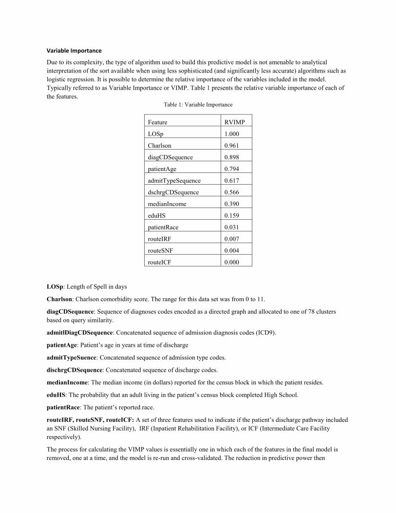
Due to its complexity, the type of algorithm used to build this predictive model is not amenable to analytical interpretation of the sort available when using less sophisticated (and significantly less accurate) algorithms such as logistic regression. It is possible to determine the relative importance of the variables included in the model. Typically referred to as Variable Importance or VIMP. Table 1 presents the relative variable importance of each of the features.

Table 1: Variable Importance

Feature RVIMP

LOSp 1.000

Charlson 0.961

diagCDSequence 0.898

patientAge 0.794

admitTypeSequence 0.617

dschrgCDSequence 0.566

medianIncome 0.390

eduHS 0.159

patientRace 0.031

routeIRF 0.007

routeSNF 0.004

routeICF 0.000

LOSp: Length of Spell in days

Charlson: Charlson comorbidity score. The range for this data set was from 0 to 11.

diagCDSequence: Sequence of diagnoses codes encoded as a directed graph and allocated to one of 78 clusters based on query similarity.

admitlDiagCDSequence: Concatenated sequence of admission diagnosis codes (ICD9).

patientAge: Patient’s age in years at time of discharge

admitTypeSuence: Concatenated sequence of admission type codes.

dischrgCDSequence: Concatenated sequence of discharge codes.

medianIncome: The median income (in dollars) reported for the census block in which the patient resides.

eduHS: The probability that an adult living in the patient’s census block completed High School.

patientRace: The patient’s reported race.

routeIRF, routeSNF, routeICF: A set of three features used to indicate if the patient’s discharge pathway included an SNF (Skilled Nursing Facility), IRF (Inpatient Rehabilitation Facility), or ICF (Intermediate Care Facility respectively).

The process for calculating the VIMP values is essentially one in which each of the features in the final model is removed, one at a time, and the model is re-run and cross-validated. The reduction in predictive power then

represents the importance of each feature. When interaction terms between features are included in the model, the process becomes more complex as groups of features must be tested. In the case of Random Survival Forest models, interaction terms are not directly included in the model formulation, rather the impact of interactions is implicitly accounted for in the branching process used to grow the large number of trees (in this case 500).

The graph encoded feature diagCDSequence, was among the top three most important variables, contributing very significantly to the predictive power of the model. As described in more detail below, the final model exhibited an average concordance index (CI) of 0.72 when diagCDSequence was included. Without this feature, the average CI dropped to 0.61. When a feature coded as the sorted and concatenated ICD-9 codes was substituted for diagCDSequence, the resulting average CI was 0.64.

Error Measurement, Model Tuning, and Performance

For statistical learning models where survival time and hazard rates are the predicted outcome or target, the underlying distributions of and are highly skewed and the data itself is right censored, error measures that compare predicted survival times to actual survival times are far too restrictive. The use of biased estimators compounds this issue. An alternative is to cast the task as one of ranking survival times rather than estimating those times outright. Individual pairs of patients can then be ranked as to which estimated time to event (readmission in this case) was shorter and then testing this against the known outcomes. This approach is a form of Concordance Index (CI) [42], which itself is related to the Mann-Whitney Parameter [43], adjusted for censored data. When applied to the test data set, a pair of patients is considered concordant if the risk of the event predicted by a model is lower for the patient who experiences the event at a later time point. The concordance probability (C-index) is the frequency of concordant pairs among all pairs of subjects. It can be used to measure and compare the discriminative power of a risk prediction models. In this setting, the concordance probabilities are weighted by the inverse of the probability of censoring in order to adjust for right censoring. Cross-validation based on bootstrap resampling or bootstrap subsampling can be applied to assess the discriminative power of various modelling strategies on the same set of data. While useful as an overall model performance measure, the CI is less useful for model tuning in which features are added and removed as small changes in predictive power are difficult to detect.

Current Model Performance

The current iteration of the model was the set of 9,461 care spells between 2013-01-01 and 2014-09-17 described earlier. The training set included 7,095 cases, with the remaining 2,366 allocated to the test set. Figure 1 presents a graph of the C-index between days 1 and 60 for the current version of the predictive algorithm. The reference model is the non-parametric Kaplan-Meier estimator. The RSF model outperforms the reference model in all but a small range of days. Performance of both models is difficult to ascertain within the first five days due to the small number of cases where patients were readmitted within that time period.

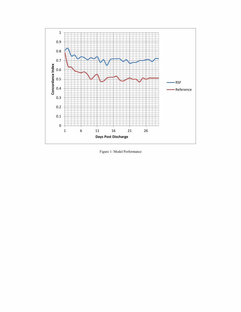
Figure 1: Model Performance

0

0.1

0.2

0.3

0.4

0.5

0.6

0.7

0.8

0.9

1

1 6 11 16 21 26

Conc

orda

nce

Inde

x

Days Post Discharge

RSF

Reference

References [1] S. F. Jencks, M. V. Williams, and E. A. Coleman, “Rehospitalizations among Patients in the Medicare

Fee-for-Service Program,” N. Engl. J. Med., vol. 360, no. 14, pp. 1418–1428, Apr. 2009. [2] H. M. Krumholz, A. R. Merrill, E. M. Schone, G. C. Schreiner, J. Chen, E. H. Bradley, Y. Wang, Y. Wang,

Z. Lin, B. M. Straube, M. T. Rapp, S.-L. T. Normand, and E. E. Drye, “Patterns of Hospital Performance in Acute Myocardial Infarction and Heart Failure 30-Day Mortality and Readmission,” Circ. Cardiovasc. Qual. Outcomes, vol. 2, no. 5, pp. 407–413, Sep. 2009.

[3] D. Kansagara, H. Englander, A. Salanitro, D. Kagen, C. Theobald, M. Freeman, and S. Kripalani, Risk Prediction Models for Hospital Readmission: A Systematic Review. Washington (DC): Department of Veterans Affairs (US), 2011.

[4] M. T. Kassin, R. M. Owen, S. Perez, I. Leeds, J. C. Cox, K. Schnier, V. Sadiraj, and J. F. Sweeney, “Risk Factors for 30-Day Hospital Readmission among General Surgery Patients,” J. Am. Coll. Surg., vol. 215, no. 3, pp. 322–330, Sep. 2012.

[5] B. J. M. Ruben Amarasingham, “An automated model to identify heart failure patients at risk for 30-day readmission or death using electronic medical record data.,” Med. Care, vol. 48, no. 11, pp. 981–8, 2010.

[6] P. J. Kaboli, J. T. Go, J. Hockenberry, J. M. Glasgow, S. R. Johnson, G. E. Rosenthal, M. P. Jones, and M. Vaughan-Sarrazin, “Associations Between Reduced Hospital Length of Stay and 30-Day Readmission Rate and Mortality: 14-Year Experience in 129 Veterans Affairs Hospitals,” Ann. Intern. Med., vol. 157, no. 12, p. 837, Dec. 2012.

[7] J. M. Glasgow, M. Vaughn-Sarrazin, and P. J. Kaboli, “Leaving Against Medical Advice (AMA): Risk of 30-Day Mortality and Hospital Readmission,” J. Gen. Intern. Med., vol. 25, no. 9, pp. 926–929, Sep. 2010.

[8] C. van Walraven, I. A. Dhalla, C. Bell, E. Etchells, I. G. Stiell, K. Zarnke, P. C. Austin, and A. J. Forster, “Derivation and validation of an index to predict early death or unplanned readmission after discharge from hospital to the community,” Can. Med. Assoc. J., vol. 182, no. 6, pp. 551–557, Apr. 2010.

[9] A. Gruneir, I. A. Dhalla, C. van Walraven, H. D. Fischer, X. Camacho, P. A. Rochon, and G. M. Anderson, “Unplanned readmissions after hospital discharge among patients identified as being at high risk for readmission using a validated predictive algorithm,” Open Med., vol. 5, no. 2, pp. e104–e111, 2011.

[10] P. E. Cotter, V. K. Bhalla, S. J. Wallis, and R. W. S. Biram, “Predicting readmissions: poor performance of the LACE index in an older UK population,” Age Ageing, vol. 41, no. 6, pp. 784–789, Nov. 2012.

[11] C. van Walraven, J. Wong, and A. J. Forster, “LACE+ index: extension of a validated index to predict early death or urgent readmission after hospital discharge using administrative data,” Open Med., vol. 6, no. 3, pp. e80–e90, 2012.

[12] J. Donzé, D. Aujesky, D. Williams, and J. L. Schnipper, “Potentially Avoidable 30-Day Hospital Readmissions in Medical Patients: Derivation and Validation of a Prediction Model,” JAMA Intern. Med., vol. 173, no. 8, p. 632, Apr. 2013.

[13] Northrup Grumman Corporation Information Systems, “Accountable Care Organization – Operational System (ACO-OS) Claim and Claim Line Feed (CCLF) Information Packet (IP) – June Release,” Centers for Medicare & Medicaid Services, NGC.ICDA.0301.04.0.0713, Jul. 2013.

[14] CMS.gov, “Readmissions Reduction Program.” CMS, 04-Nov-2015. [15] “Well Virginia ACO.” Well Virginia. [16] A. I. Arbaje, J. L. Wolff, Q. Yu, N. R. Powe, G. F. Anderson, and C. Boult, “Postdischarge

Environmental and Socioeconomic Factors and the Likelihood of Early Hospital Readmission Among

Community-Dwelling Medicare Beneficiaries,” The Gerontologist, vol. 48, no. 4, pp. 495–504, Aug. 2008.

[17] S. S. Rathore, F. A. Masoudi, Y. Wang, J. P. Curtis, J. M. Foody, E. P. Havranek, and H. M. Krumholz, “Socioeconomic status, treatment, and outcomes among elderly patients hospitalized with heart failure: Findings from the National Heart Failure Project,” Am. Heart J., vol. 152, no. 2, pp. 371–378, Aug. 2006.

[18] J. Hu, M. D. Gonsahn, and D. R. Nerenz, “Socioeconomic Status And Readmissions: Evidence From An Urban Teaching Hospital,” Health Aff. (Millwood), vol. 33, no. 5, pp. 778–785, May 2014.

[19] “University of Wisconsin Population Health Institute. County Health Rankings and Roadmaps.” 2015. [20] Census Block Conversions API. Federal Communications Commision, 2009. [21] M. Anderson, D. Antenucci, V. Bittorf, M. Burgess, M. J. Cafarella, A. Kumar, F. Niu, Y. Park, C. Ré,

and C. Zhang, “Brainwash: A Data System for Feature Engineering.,” in CIDR, 2013. [22] M. Kuhn and K. Johnson, Applied Predictive Modeling, 2013 edition. New York: Springer, 2013. [23] E. T. Lee, Statistical Methods for Survival Data Analysis, 3 edition. New York: Wiley-Interscience,

2003. [24] M. G. Akritas, “Nonparametric Survival Analysis,” Stat. Sci., vol. 19, no. 4, pp. 615–623, Nov. 2004. [25] E. L. Kaplan and P. Meier, “Nonparametric Estimation from Incomplete Observations,” J. Am. Stat.

Assoc., vol. 53, no. 282, pp. 457–481, Jun. 1958. [26] G. Cybenko, “Approximation by superpositions of a sigmoidal function,” Math. Control Signals Syst.,

vol. 2, no. 4, pp. 303–314, Dec. 1989. [27] L. Breiman, “Random Forests,” Mach. Learn., vol. 45, no. 1, pp. 5–32, Oct. 2001. [28] H. Ishwaran, U. B. Kogalur, E. H. Blackstone, and M. S. Lauer, “Random Survival Forests,” Ann. Appl.

Stat., vol. 2, no. 3, pp. 841–860, Sep. 2008. [29] N. P. Rizk, H. Ishwaran, T. W. Rice, L.-Q. Chen, P. H. Schipper, K. A. Kesler, S. Law, T. E. M. R. Lerut, C.

E. Reed, J. A. Salo, W. J. Scott, W. L. Hofstetter, T. J. Watson, M. S. Allen, V. W. Rusch, and E. H. Blackstone, “Optimum Lymphadenectomy for Esophageal Cancer:,” Ann. Surg., vol. 251, no. 1, pp. 46–50, Jan. 2010.

[30] E. Hsich, E. Z. Gorodeski, E. H. Blackstone, H. Ishwaran, and M. S. Lauer, “Identifying Important Risk Factors for Survival in Patient With Systolic Heart Failure Using Random Survival Forests,” Circ. Cardiovasc. Qual. Outcomes, vol. 4, no. 1, pp. 39–45, Jan. 2011.

[31] G.-P. Diller, A. Giardini, K. Dimopoulos, G. Gargiulo, J. Muller, G. Derrick, G. Giannakoulas, S. Khambadkone, A. E. Lammers, F. M. Picchio, M. A. Gatzoulis, and A. Hager, “Predictors of morbidity and mortality in contemporary Fontan patients: results from a multicenter study including cardiopulmonary exercise testing in 321 patients,” Eur. Heart J., vol. 31, no. 24, pp. 3073–3083, Dec. 2010.

[32] D. Fantazzini and S. Figini, “Random Survival Forests Models for SME Credit Risk Measurement,” Methodol. Comput. Appl. Probab., vol. 11, no. 1, pp. 29–45, Mar. 2009.

[33] M. A. Vedomske, D. E. Brown, and J. H. Harrison, “Random Forests on Ubiquitous Data for Heart Failure 30-Day Readmissions Prediction,” 2013, pp. 415–421.

[34] H. Ishwaran and U. B. Kogalur, “Random Survival Forests for R,” R News, vol. 7, no. 2, pp. 25–31, Oct. 2007.

[35] I. Guyon and A. Elisseeff, “An introduction to variable and feature selection,” J. Mach. Learn. Res., vol. 3, pp. 1157–1182, 2003.

[36] Richard A. Deyo, Daniel C. Cherkin, and Marcia A. Ciol, “Adapting a clinical comorbidity index for use with ICD-9-CM administrative databases,” J. Clin. Epidemiol., vol. 45, no. 6, pp. 613 – 619, 1992.

[37] C. Liu, K. Zhang, H. Xiong, G. Jiang, and Q. Yang, “Temporal skeletonization on sequential data: patterns, categorization, and visualization,” 2014, pp. 1336–1345.

[38] J. Webber, “A programmatic introduction to Neo4j,” 2012, p. 217.

[39] C. T. Have and L. J. Jensen, “Are graph databases ready for bioinformatics?,” Bioinformatics, vol. 29, no. 24, pp. 3107–3108, Dec. 2013.

[40] Neo4J. Neo Technology, 2015. [41] R. P. Yerex, “Machine Learning Based Prediction of Patient Readmission Using CMS Claims Data,”

UVA Medical System, Mar. 2015. [42] V. C. Raykar, H. Steck, B. Krishnapuram, and C. Dehing-oberije, On Ranking in Survival Analysis:

Bounds on the Concordance Index. . [43] J. A. Koziol and Z. Jia, “The Concordance Index C and the Mann–Whitney Parameter Pr(X>Y) with

Randomly Censored Data,” Biom. J., vol. 51, no. 3, pp. 467–474, Jul. 2009.