INFORMATIK BERICHTE

372 – 07/2016

A practical view on substitutions

Marija Kulaš

Fakultät für Mathematik und Informatik D-58084 Hagen

A practical view on substitutions

Marija KulasFernUniversitat in Hagen, Wissensbasierte Systeme, 58084 Hagen, Germany

marija.kulas@fernuni-hagen.de

AbstractFor logic program analysis or formal semantics, the issue of re-naming terms and generally handling substitutions is inevitable.We revisit substitutions from a practitioner’s point of view, pre-senting concepts we found useful in dealing with operational se-mantics of pure Prolog. A concept of relaxed core representation isintroduced, upon which a concept of prenaming is built. Prenam-ing formalizes the intuitive practice of renaming terms and allowsfor extensibility. A novel algorithm for term matching is proposed,which also solves the problem of substitution generality (and thusequivalence), using witness term technique. The technique aleviatesthe problem of ad-hoc proofs involving generality.

Categories and Subject Descriptors F.4.1 [Logic and constraintprogramming]

Keywords substitution, renaming, term matching, generality

1. IntroductionThe image of substitutions in logic programming research is asomewhat tainted one. First, it has been pointed out by H.-P. Ko(Shepherdson 1994, p. 148) that the original claim of strong com-pleteness of SLD-resolution needs to be rectified, because of acounter-example using the fact that

(x

f(y,z)

)is not more general

than(

xf(a,a)

), which admittedly does look rather counter-intuitive,

but complies with the definition of substitution generality (Ex-ample 6.10). Second, by composing substitutions, properties likeequivalence (Remark 6.13), idempotency (Remark 6.24), or restric-tion (Remark 6.28) are not preserved. Third, due to group structureof renamings, permuting any number of variables amounts to ”do-ing nothing”, as in

(xyyx

)∼ ε (Example 6.12). Such equivalences

are also felt to be counter-intuitive. Hence the prevalent sentimentsthat substitutions are ”quite hard matter to deal with” (Palamidessi1990) or ”very tricky” (Shepherdson 1994). In an effort to avoidsubstitutions as much as possible, resultants were proposed (Lloydand Shepherdson 1991). Still, for almost anyone embarking on ajourney of logic program analysis or formal semantics, sooner orlater the need for renaming terms and generally handling substitu-tions arises.

In the case of this author, the need arose while trying to provecompleteness of an operational semantics for pure Prolog, S1:PP

[Copyright notice will appear here once ’preprint’ option is removed.]

(Kulas 2005), and facing the following extensibility problem. Start-ing from a pair of variant queries, their respective formal deriva-tions proceed to develop. At each step, new variables may crop up,but the status of being variant should be maintained. This setup isknown from the classical variant lemma (Legacy 7.3). A new as-pect here is that we need to collect the variables, obtaining at eachstep the temporary variance between the derivations.

How to model this process of accumulating new variables andtheir correspondence between derivations? Surely by renamings?Assume the first query is p(z, u) and the second p(y, z). There isonly one relevant renaming, ρ =

(zyuzyu

). Now assume in the next

step the first derivation acquires the variable y, and the second x.The relevant renaming this time would be ρ′ =

(zyuzyxxu

). Clearly,

ρ′ is not an extension of ρ, which makes it seem unsafe to proceed:are some properties of the previous step now in danger?

For this reason, in Section 5 we introduce a slight generaliza-tion of renaming, called prenaming, which can handle extensibility(Theorem 5.17). As a bonus, it is a mathematical underpinning ofthe intuitive practice of ”renaming” terms by just considering thenecessary bindings, and not worrying whether the result is a per-mutation. In the above example that would be z 7→ y, u 7→ z. Pre-naming provides finer control of term variance, owing to relaxedcore representation, which is nothing else than allowing some x/xpairs alongside ”real” bindings, as placeholders. Prenamings relateto and are inspired by previous work as follows: A safe prenam-ing is more general than renaming for a term from (Lloyd 1987),and it maximizesW in the notion of W-renaming from (Eder 1985)(subsection 5.2). Also, prenamings can generalize substitution re-naming from (Amato and Scozzari 2009).

In Section 7, an application on a nontrivial example is shown(Lemma 7.1), where a propagation claim for logic programmingsystems has been proved, in a constructive way. As a corollary, avariant lemma (Theorem 7.4) for Prolog is obtained. Underway,we touch on the discrepancy between the rather abundant theoryof logic programming and a scarcity of mathematical claims forimplemented logic programming systems. While there are someformal proofs of properties like nominal unification (Urban et al.2004), for logic programming systems or their compilation such arestill few and far between, a notable exception being (Pusch 1996).New concepts like prenaming may help with this. In subsection 7.1we discuss the question of renaming-compatibility and resolution-compatibility of unification for logic programming systems. Suchproperties are important for formalizing operational behaviour ofProlog in a compositional way.

In Section 6, we discuss some other notions about substitutionsthat were needed in the course of work on operational semantics.A novel algorithm for term matching, also rooted in the relaxedcore idea, is proposed (Algorithm 6.1). It solves the problem ofsubstitution generality (and thus equivalence) as well, using witnessterm (Theorem 6.8). Witness term technique was also used for adirect proof of Legacy 6.27.

1 2016/6/30

2. SubstitutionFirst we need a bit of notation. Assume two disjoint sets: the setof functors, Fun, and the countably infinite set of variables, V.If W ⊆ V, any mapping F with F (W ) ⊆ V shall be calledvariable-pure on W . A mapping variable-pure on the whole set ofvariables V shall be called all-vars mapping. If V \W is finite, Wis said to be co-finite. A mapping F is injective on W , if wheneverF (x) = F (y) for x, y ∈W we have x = y.

Associated with every functor f shall be a natural number ndenoting its number of arguments, arity. To emphasize this, thenotation f /n will be used. Functors of arity 0 are called constants.Starting from V and Fun we build data objects, terms. In Prolog,everything is a term, and so shall term be here the topmost syntacticconcept. Any variable x ∈ V is a term. If t1, ..., tn are termsand f /n ∈ Fun, then f(t1, ..., tn) is a term with shape f /n andconstructor f . In case of f /0, the term shall be written withoutparentheses. If a term s occurs within a term t, we write s∈ t.

A special kind of term is dotted pair, introduced under the nameS-expression in (McCarthy 1960) and written1 as h · t, where h iscalled the head and t is called the tail of the pair. A special dottedpair is non-empty list, distinguished by its tail being a special termnil called empty list, or a non-empty list itself. In Edinburgh Prolognotation, dotted pair would be written [h|t] and empty list as [].A list of n elements is the term [t1|[t2|[...[tn|[]]]]], convenientlywritten as [t1,...,tn].

Let Vars(t) be the set of variables in the term t. A term withoutvariables is called a ground term. If the terms s and t share avariable, that shall be written s ./ t. Otherwise, we say s, t arevariable-disjunct, written as s 6./ t. The list of all variables of t, inorder of appearance, shall be denoted as VarList(t).

A recurrent theme in this paper shall be relevance, meaning”no extraneous variables” (relative to some term or terms). Thename appears in (Apt 1997, p.38), with the unary meaning, i. e.no extraneous variables relative to (one) term. This usage shall bereflected in the text as follows.

• A unifier σ of a set of equationsE (Definition 6.14, Legacy 6.27)is a relevant unifier, if Vars(σ) ⊆ Vars(E). A renaming ρembedding a prenaming α (Algorithm 5.1) is a relevant embed-ding, if Vars(ρ) ⊆ Vars(α).

Additionally, a binary version of relevance, handling two terms,shall also be needed (Algorithm 5.2, Lemma 7.1):

• A mapping F is relevant for t1 to t2, if Dom(F ) ⊆ Vars(t1)and Range(F ) ⊆ Vars(t2).

Definition 2.1 (substitution). A substitution θ is a function map-ping variables to terms, which is identity almost everywhere. Inother words, a function θ with domain Dom(θ) = V such that thefollowing requirement holds:

finite action2 The set {x ∈ V | θ(x) 6= x} is finite.

The set Core(θ) ··= {x ∈ V | θ(x) 6= x} shall be called the activedomain3 or core of θ, and its elements active variables4 of θ. Theset Ran(θ) ··= θ(Core(θ)) is called the active range of θ. The setVarsRan(θ) ··= Vars(θ(Core(θ))) is called the active variable

1 In Definition 2.1, we shall overload the dot operator with composingsubstitutions, in addition to its role as pair constructor.2 (Gallier 1986) uses the name finite support.3 Literature traditionally uses the name domain. However, in the usualmathematical sense it is always the whole V which is the domain of anysubstitution. It may be less confusing to have both the domain, which isuniformly V, and the core or active domain, making it clear that, whileevery variable can be mapped, only active variables are of interest.4 The name active variable appears in (Jacobs and Langen 1992).

range of θ. For completeness, a variable x such that θ(x) = x shallbe called a passive variable, or a fixpoint, for θ. Also, we say thatθ is active on the variables from Core(θ), and passive on all theother variables.

If Core(θ) = {x1, ..., xk}, where x1, ..., xk are pairwise dis-tinct variables, and θ maps each xi to ti, then θ shall have thecore representation {x1/t1, ..., xk/tk}, or the perhaps more visual(x1t1

...

...xktk

). Hence, the above requirement shall also be called fi-

nite core. Each pair xi/ti is called the binding for xi via θ, denotedby xi/ti ∈ θ.

Often we identify a substitution with its core representation, andthus regard it as a syntactical object, a term. So the set of variablesof a substitution is defined as Vars(θ) ··= Core(θ)∪VarsRan(θ).

The notions of restriction and extension of a mapping shall alsobe transported to core representation: if θ ⊆ σ, we say θ is arestriction of σ, and σ is an extension of θ. The restriction θ�Wof a substitution θ on a set of variables W ⊆ V is defined asfollows: if x ∈W then θ�W (x) ··= θ(x), otherwise θ�W (x) ··= x.The restriction of a substitution θ upon the variables of the termt shall be abbreviated as θ�t ··= θ�Vars(t). We also write θ�−t todenote the restriction of θ to variables outside of t, like θ�−t ··=θ�Core(θ)\Vars(t).

Definition of substitution is extended from variables to arbi-trary terms in a structure-preserving way by θ(f(t1, ..., tn)) ··=f(θ(t1), ..., θ(tn)). If s is a term, θ(s) is an instance of s via θ.

The composition θ · σ of substitutions θ and σ is defined by(θ · σ)(t) ··= θ(σ(t)). Composition may be iterated, written asσn ··= σ · σn−1 for n ≥ 1, and σ0 ··= ε. Here ε ··= () is theidentity function on V. In case an all-vars substitution ρ is bijective,its inverse shall be denoted as ρ−1. A substitution θ satisfying theequality θ · θ = θ is called idempotent.

Example 2.2.(xuwvuxvw

)·(uxvwxyyuzvwz

)=(6u6u6v6vxyyxzwwz6x6u6w6v6u6x6v6w

)=(

xyyxzwwz

).

3. RenamingDefinition 3.1 (renaming). A renaming of variables is a bijectiveall-vars substitution.

In (Eder 1985), it is synonymously called ”permutation”. Weshall reserve the word for the general case where infinite move-ments like translation are possible. Here we shall synonymouslyspeak of finite permutation due to the fact that, being a substitu-tion, any renaming has a finite core, and Legacy 3.4 holds.

From the definition of substitution, we know: if s ∈ t, thenσ(s) ∈ σ(t). For bijective substitutions (i. e. renamings), a com-plementary property holds as well:

Lemma 3.2 (renaming stability of not-in). Let ρ be a renamingand s, t be terms. If s 6∈ t, then ρ(s) 6∈ ρ(t).

Proof. Assume ρ(s) ∈ ρ(t). Then ρ−1(ρ(s)) ∈ ρ−1(ρ(t)). ♦

Corollary 3.3 (renaming stability of ”=”, ”∈”, ” 6./”). Let ρ be arenaming and s, t be terms. Then s = t iff ρ(s) = ρ(t), and alsos ∈ t iff ρ(s) ∈ ρ(t). As a consequence, s 6./ t iff ρ(s) 6./ ρ(t).

Legacy 3.4 ((Lassez et al. 1988)). A substitution ρ is a renamingiff ρ(Core(ρ)) = Core(ρ).

Legacy 3.5 ((Eder 1985)). Every injective all-vars substitution isa renaming.

So composition of renamings is a renaming. The next propertyis about cycle decomposition of a finite permutation.

2 2016/6/30

Lemma 3.6 (cycles). Let σ be an all-vars substitution. It is injec-tive iff for every x ∈ V, there is n ∈ N such that σn(x) = x.

Proof. Assume σ injective, and choose x0 ∈ V. If σ(x0) = x0,we are done. Otherwise, σi(x0) 6= σi−1(x0) for all i ≥ 1, due toinjectivity. Hence, σi−1(x0) ∈ Core(σ) for every i ≥ 1. Becauseof the finiteness of Core(σ), there is m > k ≥ 1 such thatσm(x0) = σk(x0). Due to injectivity, σm−1(x0) = σk−1(x0).By iteration we get n ··= m− k.

For the other direction, assume σ(x) = σ(y), and minimalm,nsuch that σn(x) = x, σm(y) = y. Consider the case m 6= n,say m > n. Then σm−n(y) = σm−n(x) = σm−n(σn(x)) =σm−n(σn(y)) = σm(y) = y, contradicting minimality of m.Hence m = n, and so x = σn(x) = σn(y) = y. ♦

4. Relaxed core representationIn Lemma 7.1, we shall have to deal with mappings of variablesbetween two terms. There, it is possible that a variable stays thesame, so (x, x) would have to be tolerated as a ”binding”, since weneed our mapping to cover all variables in the two terms. Therefore,we allow the set C to contain some passive variables, raising thoseabove the rest, as it were.

Definition 4.1 (relaxed core). If Core(σ) ⊆ {x1, ..., xn}, wherevariables x1, ..., xn are pairwise distinct, then {x1, ..., xn} shall becalled a relaxed core and

(x1

σ(x1)......

xnσ(xn)

)shall be called a relaxed

core representation for σ.If we fix a relaxed core for σ, it shall be denoted C(σ) ··=

{x1, ..., xn}. The associated range σ(C(σ)) we denote as R(σ).The set of variables of σ is as expected, V (σ) ··= Vars(C(σ)) ∪Vars(R(σ)). To get back to the traditional core representation, wedenote by [σ] the core representation of σ.

For extending substitution, we shall employ disjoint union.

Definition 4.2 (sum of substitutions). If σ =(x1s1

...

...xmsm

)and θ =(

y1t1

...

...yntn

)are substitutions in relaxed representation such that

{y1, ..., yn} 6./ {x1, ..., xm}, then σ ] θ ··=(x1s1

...

...xmsm

y1t1

...

...yntn

)

is the sum of σ and θ.

In case {y1, ..., yn} ./ {x1, ..., xm} but with σ(xi) = θ(yj) onany common variables xi = yj , we shall simply write σ ∪ θ. Also,we shall not be introducing special symbols to denote that σ is anextension of θ, but simply write σ ⊇ θ.

In subsection 7.2, we shall need backward compatibility of anextension. A first stab might be:

Lemma 4.3. If β(t) = t, then (α ] β)(t) = α(t).

Proof. For any x ∈ Vars(t) ∩ C(α) by definition (α ] β)(x) =α(x). Assume now x ∈ Vars(t) ∩ C(β). From the condition,β(x) = x, and by definition of extension, x 6∈ C(α), hence (α ]β)(x) = β(x) = x = α(x). Clearly, if x ∈ Vars(t) \ C(α ] β)the claim also holds. ♦

As an immediate consequence, if a substitution σ is completefor a term t, there is no danger that an extension of σ might map tdifferently from σ.

Definition 4.4 (complete for term). Let σ be given in relaxed corerepresentation. We say that σ is complete for t if Vars(t) ⊆ C(σ).

Corollary 4.5 (backward compatibility). If σ is complete for t,then for any θ holds (σ ] θ)(t) = σ(t).

5. PrenamingIn practice, one would like to change the variables in a term,without bothering to check whether this change is a permutation ornot. For example, the term p(z, u, x) can be mapped on p(y, z, x)via z 7→ y, u 7→ z, x 7→ x.

Let us call such a mapping prenaming5. Like any substitution, aprenaming α shall also be represented finitely, but in relaxed corerepresentation, in order to capture possible x 7→ x pairings. Theset C(α) is fixed by the terms to map. Obviously, injectivity isimportant for such a mapping, since p(z, u, x) cannot be mappedon p(y, y, x) without losing a variable. Hence,

Definition 5.1 (prenaming). A prenaming α is an all-vars substi-tution injective on a finite set of variables C(α) ⊇ Core(α).

Obviously, any renaming is a prenaming. For Theorem 7.4, weneed a possibility to extend a given prenaming by new bindings.

Lemma 5.2 (extension of prenaming). Let α =(x1y1

...

...xnyn

)

and β =(u1v1

...

...ukvk

)be prenamings such that {u1, ..., uk} 6./

{x1, ..., xn} and {v1, ..., vk} 6./ {y1, ..., yn}. Then α ] β =(x1y1

...

...xnyn

u1v1

...

...ukvk

)is also a prenaming.

Clearly, C(α ] β) = C(α) ] C(β) and R(α ] β) = R(α) ]R(β).

5.1 The question of inverseIn practice, a prenaming is more natural, but a ”full” renaming isbetter mathematically tractable (inverse exists). Hence we want toknow whether each prenaming can be embedded in a renaming.

The next property shows how to extend a prenaming α to obtaina renaming, and a relevant one at that, i. e. acting only on thevariables from V (α). The claim is essentially given in (Lloyd andShepherdson 1991), (Apt 1997) and (Amato and Scozzari 2009)with the emphasis on the existence6 of such an extension. In (Eder1985), the emphasis is on the actual reach7 of the extension. Thelatter is our concern as well. We formulate the claim around thenotion of prenaming, and provide a constructive proof based onLemma 3.6.

Theorem 5.3 (embedding). Let α be a prenaming. Then there is arenaming ρ which coincides with α on V\(R(α)\C(α)) such thatVars(ρ) ⊆ V (α).

Additionally, if α(x) 6= x on C(α), then ρ(x) 6= x on V (α).

Proof. If α is a prenaming, then C(α) =·· C and R(α) =·· Rare sets of n distinct variables each. We shall construct the wantedrenaming in Algorithm 5.1, where it is named α. The idea is toclose any open chains α(x), α2(x), ....

α(x) ··=

α(x), if x ∈ Cz, if x ∈ R \ C and αm(z) = x for maximal m ≤ nx, outside of C ∪R

Algorithm 5.1: Closure, the natural relevant embedding

5 Finding an appropriate name can be a struggle. Shortlisted were pre-renaming and proto-renaming.6 (Apt 1997, p. 23): ”Every finite 1-1 mapping f from A onto B can beextended to a permutation g ofA∪B. Moreover, if f has no fixpoints, thenit can be extended to a g with no fixpoints.”7 (Eder 1985, p. 35): ”Let W be a co-finite set of variables (...) and let σ be aW-renaming. Then there is a permutation π which coincides with σ on theset W.”

3 2016/6/30

Let us see if for every x there is a j such that αj(x) = x.If x ∈ C, we start as in the proof of Lemma 3.6, and considerthe sequence α(x), α2(x), .... Since C is finite, either we get twoequals (and proceed as there), or we get αk(x) 6∈ C and are stuck.For y ··= αk(x) we know α(y) = z such that αm(z) = y withmaximal m, so m ≥ k. Therefore, αm(α(y)) = y = αk(x). Dueto injectivity of α on C(α) we get αm−k(α(αk(x))) = x, andhence αm+1(x) = x.

The cases x ∈ R \C or x 6∈ C ∪R are easy. By Lemma 3.6, αis injective. By Legacy 3.5, α is a renaming. The discussion of thecase α(x) 6= x on C(α) is straightforward. ♦

Definition 5.4 (closure of a prenaming). The renaming α con-structed in Algorithm 5.1 shall be called the closure of α.

Remark 5.5 (relevant embedding is not unique). Letα =(zyuzyxw1w2

),

and let us embed it in a relevant renaming. The Algorithm 5.1gives α =

(zyuzyxw1w2

xuw2w1

). But ρ =

(zyuzyxw1w2

xw1

w2u

)is also

a relevant renaming which is embedding α. In the usual nota-tion for cycle decomposition, ρ = {(x,w1, w2, u, z, y)} andα = {(x, u, z, y), (w1, w2)}.

If we reverse the prenaming, the closure algorithm shall beclosing the same open chains but in the opposite direction, hence

Lemma 5.6 (reverse prenaming). Let α ··=(x1y1

...

...xnyn

)and β ··=(

y1x1

...

...ynxn

). Then β = α−1.

Remark 5.7 (closure is not compositional). Take α ··=(zyuzyx

)

and ρ ··=(xyyx

). Then α =

(zyuzyxxu

), ρ · α =

(zxuzxu

), ρ · α =(

zxuzxy

)and ρ · α =

(zxuzxyyu

).

Remark 5.8 (closure is not monotone). If α ⊇ α′, then not alwaysα ⊇ α′. To see this, let α =

(zyuzyx

)and α′ =

(zyuz

). Then

α′ =(zyuzyu

)and α =

(zyuzyxxu

).

5.2 Staying safeLet us look more closely into Remark 5.8: α(y) = x and α(x) =x, so y and x may not simultaneously occur in the candidate term.Otherwise, a variable shall be lost, which we call aliasing, like in(yx

)(p(x, f(y))) = p(x, f(x)).

Definition 5.9 (aliasing). Let α be a prenaming. If x 6= y butα(x) = α(y), then we say α is aliasing x and y.

So what Remark 5.8 means is: if we want to use α on a largerset than C(α), then the set Pit(α) ··= R(α) \ C(α) is dangerousto touch. But, luckily, its complement is not:

Lemma 5.10 (larger set). A prenaming α is injective on the co-finite set V \ Pit(α). The set is maximal containing C(α).

Proof. Let x, y ∈ V \ Pit(α). Is it possible that α(x) = α(y)?Possible cases: If x, y ∈ C(α), then by definition of prenamingα(x) 6= α(y). If x, y 6∈ C(α), then α(x) = x 6= y = α(y).It remains to consider the mixed case x ∈ C(α), y 6∈ C(α). Wehave α(x) ∈ R(α) and α(y) = y. So is α(x) = y possible? If yes,then y ∈ R(α), but since y 6∈ C(α), that would mean y ∈ Pit(α).Contradiction.

The set cannot be made larger: if y ∈ Pit(α), then there isx ∈ C(α) with x 6= y and α(x) = y = α(y), so injectivity iscompromised. ♦

Definition 5.11 (injectivity domain). For a prenaming α, letInDom(α) ··= V \ Pit(α). Since InDom(α) is the largest co-finite set containing C(α) on which α is injective, it shall be calledthe injectivity domain of α.

The injectivity domain of a prenaming is clearly the only safeplace for it to be mapping terms from. Hence,

Definition 5.12 (safety of prenaming). A prenaming safe8 for aterm t is a prenaming α with Vars(t) ⊆ InDom(α).

Clearly, InDom(α) = C(α) ∪ (V \ R(α)), so α is safe forits relaxed core. Hence, if α is complete for a term, it is safe forthat term. For a prenaming α with the quality R(α) = C(α), i. e.a renaming, it is no surprise that InDom(α) = V and hence safetyis guaranteed for any term.

A prenaming behaves like a renaming on its injectivity domain,since it coincides with its closure there. This follows immediatelyfrom Theorem 5.3:

Corollary 5.13 (injectivity domain). Let x ∈ InDom(α). Then

α(x) = α(x).

Corollary 5.14 (prenaming stability). A generalization of Corol-lary 3.3 holds: Let s, t be terms and α be a prenaming safe for s, t.Then s = t iff α(s) = α(t) and also s ∈ t iff α(s) ∈ α(t). As aconsequence, s 6./ t iff α(s) 6./ α(t).

Our definition of prenaming was inspired by the following moregeneral notion from (Eder 1985).

Definition 5.15 (W-renaming). Let W ⊆ V . A substitution σ is aW-renaming if σ is variable-pure on W , and σ is injective on W .

With this notion, Lemma 5.10 can be summarized as: InDom(α)is a co-finite set of variables, and the largest set W ⊇ C(α) suchthat α is a W-renaming.

What about safety of extension? If α is safe for t, α ] β doesnot have to be, even if β(t) = t, as the following example shows:α ··=

(vw

), β ··=

(zyuzyx

), t ··= p(x). The following two claims

try to redress that isssue.

Lemma 5.16 (monotonicity). Assume α ] β is defined. Then

1. InDom(α) ∪ InDom(β) = V2. InDom(α) ∩ InDom(β) ⊆ InDom(α ] β)

Proof. Since (V \ A) ∪ (V \ B) = V \ (A ∩ B)), and Pit(α) 6./Pit(β), we obtain InDom(α) ∪ InDom(β) = V.

Further, (V\A)∩ (V\B) = V\ (A∪B) and so Pit(α]β) =(R(α) ] R(β)) \ (C(α) ] C(β)) ⊆ (R(α) \ C(α)) ∪ (R(β) \C(β)) = Pit(α) ∪ Pit(β). ♦

In Remark 5.8, Pit(α′) = {y}, Pit((yx

)) = {x}, and

Pit(α) = {x}, hence InDom(α′) = V \ {y}, InDom((yx

)) =

V \ {x} and InDom(α) = V \ {x}.By the last claim, staying within InDom(α) and InDom(β)

ensures staying within InDom(α ] β). By assuming a bit moreabout α than just safety, we may ignore the nature of extension β,and still ensure safety and even backward compatibility of α ] β.This shall be used in Section 7.

Theorem 5.17 (extensibility). Assume α ] β is defined.

1. If α is safe for t and β is safe for t, then α ] β is safe for t.

8 Our definition of safe prenaming is more general than the definitionof renaming for a term in (Lloyd 1987, p. 22), since we do not requireCore(α) ⊆ Vars(t).

4 2016/6/30

2. If α is complete for t, then α] β is safe for t and (α] β)(t) =α(t).

The first part follows from Lemma 5.16 and the second from Corol-lary 4.5. Observe the importance of relaxed core for this to work:otherwise, passive bindings x/x would not be accounted for.

5.3 Variant of term and substitutionThe traditional notion of term variance, which is term renaming,shall be generalized to prenaming. As a special case, substitutionvariance is defined, inspired by substitution renaming from (Am-ato and Scozzari 2009). For this, substitution shall be regarded as aspecial case of term. The term is of course the relaxed core repre-sentation. This concept shall come in handy for proving propertiesof renamed derivations, as in subsection 7.2.

5.3.1 Term variantDefinition 5.18 (term variant). If α is a prenaming safe for t, thenwe also call α(t) a variant of t, and write α(t) ∼= t. The particularvariance and the direction of its application may be explicated:s =α t iff s = α(t).

If s ∼= t, then there is a unique α mapping s to t in a completeand relevant9 manner, i. e. mapping each variable pair and nothingelse, as computed by Algorithm 5.2. The algorithm makes do withonly one set for equations and bindings, thanks to different types.Termination can be seen from the tuple (lfun=(E), card=(E))decreasing in lexicographic order with each rule application, wherelfun=(E) is the number of function symbols in equations inE, andcard=(E) is the number of equations in E.

Start from the set E ··= {s = t} and transform according to thefollowing rules. The transformation is bound to stop. If the stopwas not due to failure, then the current set E is Pren(s, t).

elimination E ] {x = y} E, if x/y ∈ Efailure: alias E ] {x = y} failure, if (x/z ∈ E, z 6=

y) or (z/y ∈ E, z 6= x)

binding E]{x = y} E∪{x/y}, if (x/ 6∈ E) and ( /y 6∈E)

failure: instance E ] {x = t} failure, if t 6∈ V;E ] {t = x} failure, if t 6∈ V

decomposition E ] {f(s1, ..., sn) = f(t1, ..., tn)} E ∪{s1 = t1, ..., sn = tn}

failure: clash E ] {f(s1, ..., sn) = g(t1, ..., tm)} failure, if f 6= g or m 6= n

Algorithm 5.2: Computing the prenaming of s to t

Notation 5.19 (epsoid). The prenaming constructed in Algo-rithm 5.2 shall be simply called the prenaming of s to t, and denotedPren(s, t). It is complete for s and relevant for s to t.

In case s = t, we obtain for Pren(s, t) essentially the identitysubstitution. However, regarded as prenamings, Pren(t, t) and εare not the same. A prenaming α with relaxed core W mappingeach variable on itself (in other words, C(α) = W and α = ε)shall be called the W -epsoid and denoted εW . For a term t, weabbreviate εt ··= εVars(t).

Regarding composition, an epsoid behaves just like ε. Its use isfor providing completeness, and hence extensibility, by means ofplaceholding pairs x/x.

9 for prenaming, we naturally use C for Dom and R for Range.

5.3.2 Special case: substitution variantEven substitutions themselves can be renamed. To rename a sub-stitution, one regards it as a syntactical object, a set of bindings,and renames those bindings. If ρ is a renaming and σ is a sub-stitution, (Amato and Scozzari 2009) define substitution renamingby ρ(σ) ··= {ρ(x)/ρ(σ(x)) | x ∈ Core(σ)}. It is easy to seethat ρ(σ) is a substitution in core representation. For this we onlyneed two properties of ρ: variable-pure on Vars(σ) and injectiveon Vars(σ). These requirements are clearly fulfilled by prenam-ings safe on σ as well. Hence,

Definition 5.20 (substitution variant). Let σ be a substitution andlet α be a prenaming safe for σ, i. e. Vars(σ) ⊆ InDom(α). Thena variant of σ by α is

α(σ) ··= {α(x)/α(σ(x)) | x ∈ Core(σ)} (1)

We may write θ =α σ if θ = α(σ), as with any other terms.As can be expected, the concept of variance by prenaming is well-defined, owing to safety. Otherwise, the result of prenaming wouldnot even have to be a substitution again, as with α =

(yx

), σ =(

xayb

).

Lemma 5.21 (well-defined). Substitution variant is well-defined,i. e. (1) is a core representation of a substitution, and α does notintroduce aliasing.

Proof. Let Core(σ) = {x1, ..., xn}. Due to injectivity of α onVars(σ), if α(xi) = α(xj), then xi = xj , so i = j. To finishthe proof that (1) a core representation, observe x ∈ Core(σ) iffx 6= σ(x) iff α(x) 6= α(σ(x)), due to injectivity again.

Next, by Corollary 5.14, if α(σ(xi)) ./ α(σ(xj)), thenσ(xi) ./ σ(xj), meaning that α does not introduce aliasing. ♦

From Definition 5.20 and Corollary 5.13 follows

Lemma 5.22. Let σ be a substitution and α, β be prenamings suchthat α(σ) and (α · β)(σ) are defined. Then

1. (α · β)(σ) = α(β(σ))

2. α(σ) = α(σ)

For the case of ”full” renaming, there is a way to dissolve thenew expression:10

Legacy 5.23 ((Amato and Scozzari 2009)). For any renaming ρand substitution σ

ρ(σ) = ρ · σ · ρ−1

Would such a claim hold for the weakened case, prenamings?

Theorem 5.24 (substitution variant). Let σ be a substitution and αbe a prenaming safe for σ. Then

1. α(σ) · α = α · σ2. α(σ) = α · σ · α−1

Proof. First part: According to Definition 5.20, for every x ∈ Vholds (α(σ)·α)(x) = α(σ(x)). Since any substitution is structure-preserving, the claim holds for any term t as well.

Second part: From the first part we know α(σ)·α = α·σ, henceα(σ) = α · σ ·α−1. By Corollary 5.13 holds α(σ) = α(σ), whichcompletes the proof. ♦

It is known that idempotence and equivalence of substitutionsare not compatible with composition (Eder 1985). Luckily, theconcept of variance, with constant prenaming, does not share thishandicap:

10 An immediate consequence of which is ρ(σ) 6= ρ · σ.

5 2016/6/30

Theorem 5.25 (compositionality). Let σ, θ be substitutions and αbe their safe prenaming. Then

α(σ · θ) = α(σ) · α(θ)

Proof. Since Vars(σ · θ) ⊆ Vars(σ)∪Vars(θ), clearly Vars(σ · θ) ⊆InDom(α). By Theorem 5.24α(σ)·α(θ) = α·σ·α−1·α·θ·α−1 =α · σ · θ · α−1 = α(σ · θ). ♦

6. Further topicsHere is a brief overview of other substitution properties that wefound useful for analysing the operational semantics S1:PP.

For some properties like Lemma 7.1 and Theorem 7.4 we needthe concept of SLD-derivations. Regarding SLD-derivations, weshall for the most part assume traditional concepts as given in (Apt1997), but with some changes and additions outlined below. Thevariable names in actual logic programs shall be capitalized, as inProlog.Notation 6.1 (adapting SLD-derivation). Assume an SLD-derivationfor G like G ↪−.K1 :σ1 G1 ↪−.K2 :σ2 ... ↪−.Kn :σn Gn.

• Ki is here the actually used variant of a program clause (i. e.,the current input clause) and not the program clause itself.• The substitution σn · ... · σ1 shall be called the partial answer

at step n of the derivation.• Recall that a computed answer substitution (c.a.s.) for G is

defined as (σn·...·σ1)�G, wheneverGn = �. For our purposes,the restriction on the variables of G is not urgent. As an interimstep, we define a complete answer for G to be a final partialanswer, σn · ... · σ1. A c.a.s. is then a complete answer maderelevant by restricting it to query variables.

An input clauseKi obtained from a program clause K by replacingthe variables in order of appearance with A1, ..., An may be de-noted as Ki = K[A1, ..., An]. We also say that K is applicable onGi with effector clause Ki, and that Ki is effective on Gi with σi.

Showing the actually used variants of program clauses (in-stead of program clauses themselves) enables a simple definitionof derivation variables.

Definition 6.2 (variables of a derivation). Assume D to be an SLD-derivation G ↪−.K1 :σ1 G1 ↪−.K2 :σ2 ... ↪−.Kn :σn Gn. We shalldefine the set of variables of D as would be natural for a term, i. e.we regard the annotations Ki :σi as part of the derivation. Hence,Vars(D) ··= (Vars(G) ∪ ... ∪ Vars(Gn)) ∪ (Vars(σ1) ∪ ... ∪Vars(σn)) ∪ (Vars(K1) ∪ ... ∪Vars(Kn)).

One last piece of introductory notation: Head((H ← B)) ··= H .

6.1 Term matching and subsumptionConsider f(x, y) and f(z, x). Intuitively, they ”match” each other,while f(x) and g(x) do not. If asked about f(x, x) and f(x, y),we may consent that they ”match” only in one direction.

Definition 6.3 (term matching). Let g and s be two terms. If thereis a substitution σ such that σ(g) = s, then we say g matches s, andalso that s is an instance of g (as already defined in Definition 2.1).The substitution σ is then a matcher of g on s.

Moreover, if σ(g) = σ(s) = s, then we say g subsumes s. Thesubstitution σ is then a subsumer of s by g.

Example: f(x) matches f(g(x)), but does not subsume it, whilef(x, y) subsumes f(x, x). For relation to Prolog see (Neumerkel2010).

Term matching can be seen as a special case of unification,where any variables on the right-hand side are inactivated by re-placing them with new constants (hence the synonym ”one-sided

unification”). For parallel approach, see e. g. (Dwork et al. 1984).We propose a one-pass algorithm with a stress on simplicity, Algo-rithm 6.1. It decides generality and equivalence of substitutions aswell.

6.1.1 SubtermDefinition 6.4 (subterm, occurrence). A character subsequence ofthe term t which is itself a term, s, shall be called an occurrence ofsubterm s of t, denoted non-deterministically by s ∈ t. This mayalso be pictured as t = s .

Note that there may be several occurences of the same sub-term in a term. Unlike its term representation, the position (Defini-tion 6.5) of an occurrence determines it uniquely. For disambigua-tion, the n-th occurrence of s in t may be denoted as (s ∈ t)n.

Terms have a tree representation as follows. A variable x is rep-resented by the root labeled x. A term f(t1, ..., tn) is representedby the root labeled f and by trees for t1, ..., tn as subtrees, orderedfrom left to right. Thus, the root label for a term t is t itself, if t isa variable, otherwise the constructor of t.

Access path shall be defined as a variation of (Apt 1997, p. 27),and used to define pendants, which shall be needed for matching,and include disagreement pairs from (Robinson 1965).

Definition 6.5 (access path and position of subterm). Let t be aterm and consider an occurrence of its subterm s, denoted as s ∈ t.The access path of s ∈ t is defined as follows. If s = t, thenAP(s ∈ t) is the root label for t. If t = f(t1, ..., tn) and s ∈ tk,then AP(s ∈ t) ··= f/k ·AP(s ∈ tk).

By extracting the integers, we obtain the position of s ∈ t. Byextracting the labels, save for the last one, we obtain the ancestryof s ∈ t. If s1 ∈ t1 has the same position and ancestry as s2 ∈ t2,then we say s1 ∈ t1 and s2 ∈ t2 are pendants in t1 and t2. Adisagreement pair between t1 and t2 is a pair of pendants thereindiffering in the last label.

For example, let t ··= [f(y), z] and s ··= z. There is onlyone ocurrence s ∈ t. According to list definition, [f(y), z] =·(f(y), ·(z,nil)). Hence, AP(s ∈ t) = (·)/2 · (·)/1 · z, so theposition of s ∈ t is 2 · 1 and its ancestry is (·) · (·). An exampleof pendants: f(y) ∈ [f(y), z] and g(a, b) ∈ [g(a, b), h(x)]. This isalso a disagreement pair.

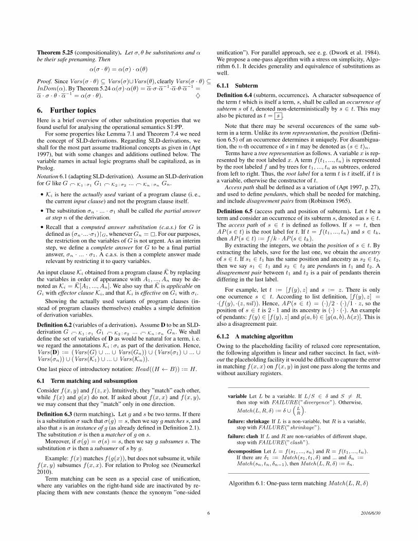
6.1.2 A matching algorithmOwing to the placeholding facility of relaxed core representation,the following algorithm is linear and rather succinct. In fact, with-out the placeholding facility it would be difficult to capture the errorin matching f(x, x) on f(x, y) in just one pass along the terms andwithout auxiliary registers.

variable Let L be a variable. If L/S ∈ δ and S 6= R,then stop with FAILURE(”divergence”). Otherwise,

Match(L,R, δ) ··= δ ∪(LR

).

failure: shrinkage If L is a non-variable, but R is a variable,stop with FAILURE(”shrinkage”).

failure: clash If L and R are non-variables of different shape,stop with FAILURE(”clash”).

decomposition Let L = f(s1, ..., sn) and R = f(t1, ..., tn).If there are δ1 ··= Match(s1, t1, δ) and ... and δn ··=Match(sn, tn, δn−1), then Match(L,R, δ) ··= δn.

Algorithm 6.1: One-pass term matching Match(L,R, δ)

6 2016/6/30

Theorem 6.6 (matching). Algorithm 6.1 solves the problem ofmatching L on R: If Match(L,R, ε) stops with failure, then Ldoes not match R; otherwise, it stops with a substitution δ suchthat [δ] is a relevant matcher of L on R. This follows from

1. If Match(L,R, δ) stops with failure, there is no µ with µ(L) =R and µ ⊇ δ.

2. If Match(L,R, δ) = δ′, then δ′(L) = R and δ′ ⊇ δ. Inother words, Match(L,R, δ) is a matcher of L on R con-taining δ. Additionally, δ′ is complete for L and Vars(δ′) ⊆Vars((L,R, δ)).

Proof. This algorithm clearly always terminates. For the Proof of 1,we need two observations, readily verified by structural induction:

• If µmaps L onR, then it maps any s ∈ L on its pendant t ∈ R.• Each time the algorithm visits one of the cases, the registersL and R denote either the original terms, or some pendantstherein.

Thus, in the two middle non-variable cases there can be no matcherfor the original terms, notwithstanding δ.

In the variable case, the purported matcher µwould have to mapone variable on two different terms (Figure 1).

x x?−−−−−→ s r

Figure 1. Divergence: one variable, two terms

Proof of 2: By structural induction. In case of variable, the claimholds. Assume we have a case of decomposition and the claimholds for the argument terms, i. e. δ1(s1) = t1, δ1 ⊇ δ, δ2(s2) =t2, δ2 ⊇ δ1, ..., δn(sn) = tn, δn ⊇ δn−1, and each δiis complete for si as well as relevant. Due to completeness andCorollary 4.5, from δn ⊇ ... ⊇ δ2 ⊇ δ1 follows δn(s1) = ... =δ2(s1) = t1 and so forth. Hence, δn(L) = R. Clearly, δn ⊇ δ andδn is complete for L and relevant. As a final detail, recall that δnmay contain passive pairs x/x, which are eliminated in [δn]. ♦

6.2 GeneralityAs an application of the matching algorithm Algorithm 6.1, wecan solve the problem of generality and equivalence between twosubstitutions.

Definition 6.7 (more general). A substitution σ is more general (orless instantiated)11 than a substitution θ, written as σ ≤ θ,12 if σis a right-divisor of θ, i. e. if there exists a substitution δ with theproperty θ = δ · σ.

How to check whether σ ≤ θ? One possibility would be tolook for a counter-example, i. e. try to find a term w such thatfor no renaming δ holds δ(σ(w)) = θ(w). Let us call such aterm a witness term. How to obtain a witness term? Intuitively,we may take w to be the list of all variables of σ, θ, denotedw ··= VarList((σ, θ)), and see if we can find an impasse, i. e.some parts of σ(w) that cannot possibly simultaneously be mappedon the respective parts of θ(w). It turns out this is sufficient.

Theorem 6.8 (witness). σ ≤ θ iff for some w with Vars(w) =Vars((σ, θ)) holds that σ(w) matches θ(w).

11 It has also been said that σ schematises θ (Huet 1976).12 Some authors like (Jacobs and Langen 1992) and (Amato and Scozzari2009) turn the symbol ≤ around. Indeed the choice may appear to beabitrary. But we shall stick to the notion that a more general object is”smaller”, because it correlates with the ”smallness” of the substitutionstack.

Proof. If δ · σ = θ, then surely δ(σ(w)) = θ(w).For the other direction, assume there is µ with µ(σ(w)) =

θ(w). By Theorem 6.6, we can choose the matcher µ to be relevant,so Vars(µ) ⊆ Vars((σ, θ)). If for some x ∈ V holds µ(σ(x)) 6=θ(x), then clearly x 6∈ Vars((σ, θ)), hence the inequality becomesµ(x) 6= x, meaning x ∈ Core(µ), which is impossible. ♦

As a consequence, we obtain a simple visual criterion.

Corollary 6.9 (witness). The relation σ ≤ θ does not hold, iff forsome w with Vars(w) ⊆ Vars((σ, θ)) any of the following holds:

1. At some corresponding positions, σ(w) exhibits a non-variable,and θ(w) exhibits a variable (”shrinkage”), or a non-variableof a different shape (”clash”).

2. σ(w) exibits two occurrences of variable x, but at the cor-responding positions in θ(w) there are two mutually distinctterms (”divergence”).

The search for an impasse can be performed by Algorithm 6.1via Match(σ(w0), θ(w0), ε), where w0 ··= VarList((σ, θ)).

If no impasse is found, the algorithm produces δ such thatθ = δ · σ. Some test runs are in Figure 2 and Figure 3.

Example 6.10. The subtlety of the relation ”more general” isillustrated in (Apt 1997) with the following example: σ ··=

(xy

)is

more general than(xaya

), but not more general than θ ··=

(xa

). The

former claim is justified by(xaya

)=(ya

)·(xy

). The matcher was

here not difficult to guess, but in general may be, and can alwaysbe found by Algorithm 6.1 (Figure 2).

The latter is a simplified form of a counter-example by Hai-Ping Ko (reported in (Shepherdson 1994)), which was pivotal inshowing that the strong completeness theorem for SLD-derivationfrom (Lloyd 1987) needed a revision. The Ko example purportsthat σ ··=

(x

f(y,z)

)is not more general than θ ··=

(x

f(a,a)

),

where y, z are distinct variables. For proof, it was observed: ifδ ·(

xf(y,z)

)=(

xf(a,a)

), then y/a, z/a ∈ δ, therefore even if one

of y, z is equal to x, at least one of bindings y/a, z/a has to be inδ ·(

xf(y,z)

). To aleviate the need for such ”ad-hoc”, custom-made

proofs, Algorithm 6.1 could be used, giving divergence (Figure 3).

[x, y]

+����σ =

(xy

)QQQQ

θ =(xa

ya

)

s[y, y]

δ =(ya

) → [a, a]

Figure 2. Successfull check on ≤

6.3 EquivalenceThe set of substitutions is not partially ordered by ≤, namely it ispossible that σ ≤ θ and θ ≤ σ for σ 6= θ. Such cases form anequivalence relation, called simply equivalence13 and denoted byσ ∼ θ.

The following property, in similar form, has been proven in(Eder 1985); the formulation is from (Apt 1997). The propertyfollows from Theorem 6.8 as well, since the case where one of apendant pair is a variable and the other a non-variable is clearly notpossible (shrinkage failure).

13 perhaps a new name like equigeneral would be less confusing, in view ofcounter-intuitive equivalences?

7 2016/6/30

[x, y]

+����σ =

(xa

) QQQQ

θ =(

xy

)

s[a, y] ×

shrinkage

→ [y, y]

[x, y, z]

+����σ =

(x

f(y,z)

)QQQQ

θ =(

xf(a,a)

)

s[f(y, z), y, z] ×

divergence

→ [f(a, a), y, z]

[x, y]

+����σ =

(x

f(y)

)QQQQ

θ =(

xg(y)

)

s[f(y), y] ×

clash

→ [g(y), y]

Figure 3. Failed check on ≤

Legacy 6.11 (equivalence). θ is more general than θ′ and θ′ ismore general than θ iff for some renaming ρ such that Vars(ρ) ⊆Vars(θ) ∪Vars(θ′) holds ρ · θ = θ′.

With some practice, such a renaming ρ can be guessed, orsimply constructed by Algorithm 6.1.

Example 6.12. Since(yxxy

)is a renaming and

(yxxy

)·(yxxy

)= ε,

we have(yxxy

)∼ ε. In other words, if we permute two variables,

that amounts to ”doing nothing”. This is a much-cited exampleof counter-intuitive character of equivalence. In fact, due to groupstructure of finite permutations, any two renamings are bound to beequivalent, so permuting any number of variables amounts to doingnothing.

Remark 6.13 (”∼” is not compositional). Equivalence is not com-patible with composition, as shown in (Eder 1985): Let σ ··=

(yx

),

σ′ ··=(xy

)and θ ··=

(xz

). Then σ ∼ σ′, but θ · σ =

(yzxz

)6∼

θ · σ′ =(xy

). The non-equivalence is verified by Algorithm 6.1.

6.4 UnificationDefinition 6.14 (unification). Let s and t be terms. If there is asubstitution θ such that θ(s) = θ(t), then s and t are said to beunifiable, and θ is their unifier, the set of all such being Unif (s, t).It is a relevant, if Vars(θ) ⊆ Vars(s) ∪ Vars(t). A unifier θ ofs and t is their most general unifier (mgu), if it is more generalthan any other unifier; the set of all such is Mgus(s, t) ··= {θ ∈Unif (s, t) | for every α ∈ Unif (s, t) holds θ ≤ α}.

A set of equations {a1=b1, ..., an=bn} may be condensedto one equation like f(a1, ..., an)=f(b1, ..., bn), and vice versa,which shows that unifying two terms and unifying arbitrarily manyterms are the same task. So the notions of unifier and mgu canbe extended from a single equation s=t to a set of equations Eby defining Unif (E) ··= {θ | for every (s=t) ∈ E holds θ(s) =θ(t)}. Similarly for Mgus(E). A set of equations is in solved formif it is of the form {x1=t1, ..., xn=tn} where all xi are distinctand none of them occurs in any tj .

If σ ∈ Mgus(s, t), then for any renaming ρ by Corollary 3.3ρ · σ ∈ Mgus(s, t). In fact, any element from Mgus(s, t) has thisform, as a consequence of Legacy 6.11:

Legacy 6.15 (equivalence of mgus). Let µ ∈ Mgus(E). Thenµ′ ∈ Mgus(E) iff there is a renaming ρ such that Vars(ρ) ⊆Vars(µ) ∪Vars(µ′) and µ′ = ρ · µ.

Thus, the set Mgus(s, t) is either empty or infinite.14 As a meta-function, Mgus has two pleasing properties: it is compatible withrenaming and it is compatible with LD-resolution.

Lemma 6.16 (renaming compatibility of Mgus). For every ρ andE holds Mgus(ρ(E)) = ρ(Mgus(E)).

Proof. This follows from Theorem 5.24 and Corollary 3.3. Assumeσ ∈ Mgus(s, t), then ρ(σ)(ρ(s)) = ρ(σ(s)) = ρ(σ(t)) =ρ(σ)(ρ(t)). Further, if θ is a unifier of ρ(s), ρ(t), then θ · ρ is aunifier of s, t, hence there is a renaming δ with θ · ρ = δ ·σ, givingθ = δ · σ · ρ−1 = δ · ρ−1 · ρ · σ · ρ−1 = (δ · ρ−1) · ρ(σ),meaning ρ(σ) ∈ Mgus(ρ(E)). For the other direction, observeθ = ρ · ρ−1 · δ · σ · ρ−1 = ρ(ρ−1 · δ · σ). ♦

Compatibility of Mgus with LD-resolution, also called iterationproperty, is proved in (Apt 1997).

Legacy 6.17 (iteration for Mgus). 1. Let E1, E2 be sets of equa-tions. If σ is a mgu of E1 and θ is a mgu of σ(E2), then θ · σ isa mgu of E1 ∪ E2.

2. Moreover, if E1 ∪ E2 is unifiable, then there exists a mgu σ ofE1, and for each such σ there exists a mgu θ of σ(E2).

6.4.1 Unification by algorithmFor any two unifiable terms s, t holds that Mgus(s, t) is an infi-nite set. On the other hand, any particular unification algorithm Aproduces, for the given two unifiable terms, just one deterministicvalue as their mgu. We shall denote this particular mgu of s and tas A(s, t), the algorithmic (or concrete) mgu of s and t, producedby algorithm A.

The task of unification was introduced and solved in (Robin-son 1965). Another classical unification algorithm is (Martelli andMontanari 1982), based on (Herbrand 1930), The algorithm is usu-ally given in non-deterministic form, here denoted as Am2, but itcan be made deterministic using sequences instead of sets and pick-ing the leftmost equation eligible for a rule application, as observedin (Apt 1997, p. 36). The resulting algorithm shall be denoted Am2.

6.4.2 ... and iteration propertyAs opposed to Mgus , any particular unification algorithm like Am2

does not have to satisfy the iteration property. But the deterministicversion Am2 does.

Example 6.18 (no iteration for Am2). Let E1 ··= (x=y, y=x)and E2 ··= (z=f(x)). If we pick the equation y=x for bind-ing (denoted by underlining), we obtain E1 = {x=y, y=x} {x=x, y=x} {y=x}

(yx

)=·· σ and σ(E2)

(z

f(x)

)=··

θ. However, for unifying E1 ∪ E2 we may as well pick x=yfor binding, and get E1 ∪ E2 = {x=y, y=x, z=f(x)} {x=y, y=y, z=f(y)}

(xy

zf(y)

)6= θ · σ.

Lemma 6.19 (iteration for Am2). Assume σ = Am2(E′) andθ = Am2(σ(E′′)). Then Am2((E′, E′′)) = θ · σ.

Proof. By Legacy 6.17, we know that E′, E′′ is unifiable.The deterministic version of Am2 transforms an equation se-

quence from left to right. This has the nice consequence that Am2

chooses the same equations to transform in E′ as in E′, E′′ for so

14 Because of the equivalence, the sloppy formulation ”the most generalunifier of s and t” is often used.

8 2016/6/30

long as E′ has not reached its solved form. The only interestingsteps here are binding steps. Underlined is the next candidate forbinding, which is afterwards shaded, to signify that this pair nowwent ”passive”, i. e.it cannot be elected for further transformationsand may merely get its right-hand side further instantiated.

Am2((E′, E′′)) = Am2((x1=t1, E′1, E

′′))

= Am2((x1=t1 , σ1(E′1), σ1(E′′))

= Am2((x1=t1 , x2=t2, E′2, σ1(E′′)))

= Am2((σ2(x1=t1) , x2=t2 , σ2(E′2), σ2(σ1(E′′))))

= ... = Am2(( (σk · ... · σ2)(x1=t1) , ..., σk(xk−1=tk−1) , xk=tk,

(σk · ... · σ1)(E′′))) = Am2((x1=(σk · ... · σ2)(t1) , ...,

xk−1=σk(tk−1) , xk=tk, (σk · ... · σ1)(E′′)))

where σ1 =(x1t1

), ..., σk =

(xktk

). Here we made use of

x1 6∈ σ1(E′1) meaning x1 6./ σ2, and x1, x2 6∈ σ2(E′2) mean-ing x1, x2 6./ σ3, etc., which are due to definition of binding steps.Putting E′′ = �, we obtain solved form, hence

σ = Am2(E′) =

(x1

(σk · ... · σ2)(t1)

...

...

xk−1

σk(tk−1)

xktk

)

=

(xktk

)·(xk−1

tk−1

)· ... ·

(x1t1

)= σk · ... · σ1

Consider now an arbitrary E′′. From the definition of bindingsteps follows that x1, ..., xk 6./ (σk · ... · σ1)(E′′) = σ(E′′),which shows that the pairs from the solved form for E′ remainpassive during the handling of σ(E′′). Thus, Am2((E′, E′′)) =θm · ... · θ1 · σk · ... · σ1, where θ1, ..., θm stem from bindingsteps for σ(E′′), and θ = Am2(σ(E′′)) = θm · ... · θ1. Overall,Am2((E′, E′′)) = θ · σ, as hoped for. ♦

6.4.3 ... and renaming-compatibilityFor freely choosable mgus, renaming-compatibility holds, as seenin Lemma 6.16. But what if mgus are chosen by an algorithm? Forexample, the simplest unification problem p(x) = p(y) has amongothers two equally attractive candidate mgus, {x/y} and {y/x}.Assume our unification algorithm decided upon {x/y}. Assumefurther that we rename the protagonists and obtain the unificationproblem p(x) = p(z). What mgu shall be chosen this time? Toensure some dependability in this issue, we shall place on anyunification algorithm the following simple requirement.

Axiom 6.20 (renaming compatibility of A). Let A be a unificationalgorithm. For any renaming ρ and any equation E, it has to holdA(ρ(E)) = ρ(A(E)).

Since classical unification algorithms like Robinson’s andMartelli-Montanari’s do not depend upon the actual names of vari-ables15, this requirement is in praxis always satisfied.

Deterministic character of unification algorithms allows forsome predictability when applying a program clause on a queryin different ways, i. e. using different variants. This is expressedin the first part of our next claim. The second part makes a con-nection between any resolution for a query, and the one made withalgorithm A.

Lemma 6.21 (two input clauses). Assume a unification algorithmA satisfying Axiom 6.20. Let G be a query and K and L be twovariants of the same program clause for G, each variable-disjunctwith G. Let λ ··= Pren(K,L). Then

15 as remarked in (Amato and Scozzari 2009)

1. there is A(G=Head(L)) = θ iff there is A(G=Head(K)) =

λ−1

(θ)

2. K is effective onG with some mgu σ iff there is renaming ρ withθ = ρ · λ(σ)

Additionally, if σ is relevant, then λ(σ) = λ(σ). If furthermore Aproduces relevant mgus, then Vars(ρ) ⊆ Vars(G) ∪Vars(L).

Proof. For the first part, λ(A(G=Head(K))) = A(λ(G=Head(K)))= A(λ(G)=λ(Head(K)))) = A(G=Head(L)), which is dueto Axiom 6.20, λ(G) = G and λ(K) = L. Hence, if θ ··=A(G=Head(L)), then A(G=Head(K)) = λ

−1(θ).

For the second part, note that σ and A(G=Head(K)) are twomgus for the same unification task. Hence, by Legacy 6.15, there isrenaming δ with

Vars(δ) ⊆ Vars(σ) ∪Vars(A(G=Head(K))) (2)

such that A(G=Head(K)) = δ · σ. From λ−1

(θ) = δ · σ we getθ = λ(δ) · λ(σ). By assigning ρ ··= λ(δ) we obtain the claim.

It remains to consider relevance. If σ is relevant, Vars(σ) ⊆Vars(K) ∪ Vars(G). On the other hand, Pit(λ) = Vars(L) \Vars(K) and G 6./ L, hence Pit(λ) 6./ σ, meaning that λ(σ) isdefined and λ(σ) = λ(σ). Lastly, if both σ and A(G=Head(K))are relevant, from (2) follows Vars(ρ) ⊆ Vars(G)∪Vars(L). ♦

Notation 6.22 (equivalent modulo prenaming). If for some prenam-ing λ holds θ ∼ λ(σ), then we also write θ ∼λ σ.

With this notation, in the previous claim we would have hadθ ∼λ σ. Assuming relevant mgus, this can be further simplified toθ ∼λ σ.Remark 6.23. The relationship from Lemma 6.21 is symmetrical.Let µ ··= Pren(L,K), then µ = λ

−1(Lemma 5.6). From θ =

ρ · λ(σ) follows λ−1

(ρ−1 · θ) = σ. By assigning δ ··= λ−1

(ρ−1)we obtain σ = δ · µ(θ), or σ ∼µ θ.

If θ is relevant, Vars(θ) ∈ Vars(G,L), so due to G 6./ Kand Pit(µ) = Vars(K) \ Vars(L) we have θ 6./ Pit(µ), thusµ(θ) = µ(θ), and σ ∼µ θ.

6.5 IdempotenceRecall that a substitution θ satisfying the equality θ ·θ = θ is calledidempotent. Any two unifiable terms have an idempotent (and rel-evant) most general unifier, as provided by classical unification al-gorithms.Remark 6.24 (idempotence is not compositional). As illustratedby (Eder 1985), composition of two idempotent substitutions doesnot have to be idempotent – not even equivalent to an idempotentsubstitution. Example: σ ··=

(x

f(y)

)and θ ··=

(y

f(z)

)give

σ · θ =(

xf(y)

yf(z)

).

However, θ · σ =(

xf(f(z))

yf(z)

)is idempotent. This is an

instance of a useful property from (Apt 1997).

Legacy 6.25 (two idempotence criteria). Let σ, θ be substitutions.

1. θ is idempotent iff Core(θ) ∩VarsRan(θ) = ∅.2. Let σ and θ be idempotent. If VarsRan(θ) 6./ Core(σ), thenθ · σ is also idempotent.

The first criterion is quite intuitive: if the active domain andthe active range of a substitution σ have no variables in common,then all the variables from the active domain shall be released fromthe term t after the application of σ upon t. Therefore, a repeatedapplication of σ cannot change anything.

9 2016/6/30

By the unruly charm of substitutions,(xyyx

)is an mgu for

t = t, yet surely not the expected one. It is lucky that idempotencyprevents such surprises:

Lemma 6.26 (pertinence). If σ is idempotent and σ ∈ Mgus(t, t)for some t, then σ = ε.

Proof. Since we know that ε ∈ Mgus(t, t), by Legacy 6.15 therehas to hold ε ∼ σ, so there is a renaming ρ such that ρ = ρ ·ε = σ.If σ is idempotent, by Legacy 6.25 we know that Core(σ) ∩VarsRan(σ) = ∅. The only renaming with this property is ε, sincefor a renaming always holds Core = Ran (Legacy 3.4). ♦

It turned out that relevance is a mandatory property of an idem-potent mgu (Apt 1997). This shall come in handy for subsec-tion 7.2. We give a direct proof using witness term.

Legacy 6.27 (relevance). Every idempotent mgu is relevant.

Proof. Assume σ ∈ Mgus(E) is idempotent, but not relevant, i. e.there is z ∈ Vars(σ) such that z 6∈ Vars(E). Let us show thatσ cannot be an mgu, by finding a unifier θ of E such that σ 6≤ θ.Technically, we construct θ and a witness term w such that for noδ can hold δ(σ(w)) = θ(w), as outlined in Corollary 6.9.

Case z ∈ Core(σ): Here we choose θ ··= σ�−z . If σ is anidempotent unifier of E, then so is θ (Legacy 6.25).

Subcase 1: σ(z) = g is ground. Since θ(z) = z, the witnesscan be w ··= z (shrinkage). Subcase 2: σ(z) contains a variable,say x, pictured as σ(z) = x . Due to idempotency of σ, holdsx 6∈ Core(σ), so x 6= z. We get σ([x, z]) = [x, x ], whereasθ([x, z]) = [x, z] = [x, 6x ]. So with w ··= [x, z] we havedivergence (if σ(z) = x) or shrinkage (otherwise).

Case z 6∈ Core(σ), but z ∈ Ran(σ): There is x ∈ Core(σ)(and therefore x 6= z) such that σ(x) = z . Here we take θ tobe an idempotent and relevant mgu of E (e. g. the outcome of aclassical unification algorithm). Due to relevance, z 6∈ θ(x). We getσ([z, x]) = [z, z ], whereas θ([z, x]) = [z, 6z ] (divergence). ♦

6.6 RestrictionRemark 6.28 (restriction is not compositional). In general, (σ ·θ)�W = σ�W · θ�W does not hold. Take θ ··=

(xy

), σ ··=

(ya

),

W ··= {x}. Then σ · θ =(ya

)·(xy

)=(xaya

), (σ · θ)�W =

(xa

),

but on the other hand, σ�W = ε, θ�W = θ, σ�W · θ�W =(xy

).

On the plus side, restriction is renaming-compatible: ρ(σ�W ) =ρ(σ)�ρ(W ). Also, by Legacy 6.25, any restriction of an idempotentsubstitution is itself idempotent.

7. Claims for logic programming systemsLooking for the meaning of logic programming, there are three lev-els to consider: logical level, which is Horn-clause logic (HCL) andits extensions; proof method, based on SLD-resolution, for han-dling the question of logical consequence for HCL; and implemen-tation level, which uses fixed algorithms for mgu, standardization-apart and search. The first two levels have been extensively stud-ied and it is known that SLD-resolution and its special case LD-resolution are handling the question of logical consequence in asound and complete way for HCL. The third level is by its naturemore a subject of technical than of theoretical interest. The latterseems to have culminated in the assertion that the usual search strat-egy of Prolog, depth-first search, is incomplete. Yet, it is our beliefthat there is an interesting theoretical side to the logic programmingsystems as well.

7.1 Compatibility claims: partly preservedImplementing logic programming means that the freedom of Hornclause logic must be restrained:

• most general unifier is provided by a fixed algorithm A

• standardization-apart is provided by a fixed algorithm S

7.1.1 Renaming-compatibilityIf we have an SLD-derivation, it is now not possible to just renameit wholesale (the resolvents, the mgus, the input clauses), whichwas possible in Horn clause logic, by virtue of Corollary 3.3. Thisis because the two fixed algorithms do not have to be renaming-compatible – in fact, the second one cannot be.

To see this, assume a standardization-apart algorithm has forthe query G ··= p(X ,Y ) at the tip of a derivation D assignedthe input clause K ··= ”p(U ,V )← q(U ,W ).”. With renam-ing ρ =

(UW

WU

), and assuming the algorithm is renaming-

compatible, the query ρ(G) = G at the tip of the derivationρ(D) = D would need to be assigned the input clause ρ(K) =”p(W ,V )← q(W ,U ).”. But already something else has beenassigned to it.

As a consequence, the handling of local variables (subsec-tion 7.2) shall require some more attention.

7.1.2 Resolution-compatibility (”iteration property”)As seen in subsubsection 6.4.1, Am2 does not but Am2 does satisfythe iteration property. The iteration property (or resolution com-patibility) states that the particular unification algorithm works thesame as the LD-resolution algorithm on a sequence of equationsrepresented via predicate eq/2 defined as ”eq(X ,X ).”.

Iteration property is important for compositional formal seman-tics of logic programming like S1:PP.

7.2 Variant lemma revisitedFor logic programming implementations complying with Ax-iom 6.20 and yielding relevant mgus, that is to say for all of them,16

a propagation result can be proved, which leads to a constructiveand incremental version of the variant lemma.

Assume the program ”son(S)← male(S), child(S ,P).”,and let us enquire about son in two derivations (Table 1). If weknow that one query, say son(X ), is a variant of the other, son(A),does the same connection hold between the resolvents as well?

As can be seen from Table 1, in a resolution some new vari-ables may crop up, originating from standardization-apart in caseswhere the clause body has variables not present in the head. For thepurposes of this paper let us call them local variables, as opposedto query variables. Were it not for local variables, the resolventsin both derivations would clearly be variants, with the same pre-naming as for the original queries. Yet, even though the variablesnew in one derivation do not have to be new in the other (Table 1),at least the prenaming can be extended to accomodate those localvariables. The claim is proved in a constructive manner.

query

son(X )son(A)

input clause

son(B)← male(B), child(B ,A).son(X )← male(X ), child(X ,B).

resolvent

male(X ), child(X ,A)male(A), child(A,B)

Table 1. Resolution may produce local variables

16 Classical unification algorithms not only satisfy Axiom 6.20 butalso yield idempotent mgus. Idempotent mgus are always relevant(Legacy 6.27).

10 2016/6/30

Lemma 7.1 (propagation of variance). Assume a unification algo-rithm A satisfying Axiom 6.20. Assume an SLD-derivation D end-ing with G and an SLD-derivation D′ ending with G′ such thatα(G) = G′ for some prenaming α which is complete for G andrelevant for D to D′.

Further assume that G ↪−.K :σ H and G′ ↪−.K′ :σ′ H ′ suchthat in G and G′ atoms in the same positions were selected andK,K′ are variants of the same program clause. Lastly assume thatσ is a relevant mgu. Then for λ ··= Pren(K,K′) holds

1. α ] λ is complete for H

2. α ] λ is relevant for D ↪−.K :σ H to D′ ↪−.K′ :σ′ H ′

3. σ′ = (α ] λ)(σ) and H ′ = (α ] λ)(H)

The claim can be summarized in Figure 4, and the role ofrelevance in Figure 5.

G↪−.−−−−−→ H

α

yα]λyα]λ

G′ −−−−−→↪−.

H ′

Figure 4. Propagation of variance

son(X )↪−.−−−−−→ male(X ), child(X ,A)

yα=(XA

AC )

yα] ?

son(A) −−−−−→↪−.

male(A), child(A,B)

Figure 5. ...is not always possible

Proof. First let us establish that α ] λ is defined. Due to relevanceof α for D,D′,

C(α) ⊆ Vars(D) and R(α) ⊆ Vars(D′) (3)

Due to standardization-apart, K 6./ D and K′ 6./ D′, hence

C(λ) 6./ D and R(λ) 6./ D′ (4)

Thus C(α) 6./ C(λ) and R(α) 6./ R(λ), so α ] λ is defined. Also,(4) proves that λ is passive on old variables, i. e. λ(D) = D.

LetG ··= (M, A,N) andH ··= σ(M, B,N), where M,N areconjunctions. Then G′ = (M′, A′,N′) = (α(M), α(A), α(N)).

Let K : A1 ← B1 and K′ : A2 ← B2. Then σ = A(A,A1),B = σ(B1) and σ′ = A(A′, A2), B′ = σ′(B2). Also,

Vars(M, A,N) ⊆ C(α), by completeness of α for G (5)Vars(K) = Vars(A1, B1), by definition of λ (6)Vars(σ) ⊆ Vars(A) ∪Vars(A1), by relevance of σ (7)

Having thus fielded all the assumptions, we obtain

Vars(M, A,N) ⊆ InDom(α ] λ), by (5) and Theorem 5.17(8)

Vars(A1, B1) ⊆ InDom(α ] λ), by (6) and Theorem 5.17 (9)Vars(σ) ⊆ InDom(α ] λ), by (7), (8) and (9) (10)

(α ] λ)(σ) = (α ] λ)(σ), by (10) (11)

Proof of 3:

σ′ = A(A′, A2) = A(α(A), λ(A1))

= A((α ] λ)(A), (α ] λ)(A1)), by (5), (6) and Theorem 5.17

= A((α ] λ)(A), (α ] λ)(A1)), by (8) and (9)

= (α ] λ)(A(A,A1)), by Axiom 6.20

= (α ] λ)(σ) = (α ] λ)(σ), by (11)

B′ = σ′(B2) = (α ] λ)(σ)(λ(B1))

= (α ] λ)(σ)((α ] λ)(B1)), by (6) and Theorem 5.17= (α ] λ)(σ(B1)), by Theorem 5.24= (α ] λ)(B)

H ′ = σ′(α(M), B′, α(N))

= (α ] λ)(σ)(α(M), (α ] λ)(B), α(N))

= (α ] λ)(σ)((α ] λ)(M), (α ] λ)(B), (α ] λ)(N)), by (5)= (α ] λ) · σ(M, B,N), by Theorem 5.24= (α ] λ)(H)

Proof of 2: By definition, C(λ) = Vars(K) and R(λ) =Vars(K′). Hence, and due to relevance of α, C(α ] λ) =C(α) ] C(λ) ⊆ Vars(D) ∪ Vars(K) ⊆ Vars(D ↪−.K :σ H).Similarly, R(α ] λ) ⊆ Vars(D′ ↪−.K′ :σ′ H ′), therefore α ] λ isrelevant for D ↪−.K :σ H to D′ ↪−.K′ :σ′ H ′.

Proof of 1: By (5) and (6), Vars(H) ⊆ Vars(G) ∪ Vars(K) ⊆C(α)∪C(λ) = C(α]λ), meaning α]λ is complete for H . ♦

Definition 7.2 (similarity). SLD-derivations of the same lengthG ↪−.K1 :σ1 G1 ↪−.K2 :σ2 ... ↪−.Kn :σn Gn

G′ ↪−.K′1 :σ′

1G′1 ↪−.K′

2 :σ′2... ↪−.K′

n :σ′nG′n

(12)

are similar if G and G′ are variants and additionally at each step iholds: atoms in the same position are selected, and the input clausesKi and K′i are variants of the same program clause.

That the name ”similarity” is justified, follows from the claimknown as variant lemma ((Lloyd 1987), (Lloyd and Shepherdson1991), (Apt 1997)), here in the formulation from (Doets 1993).

Legacy 7.3 (variant). Finite derivations which are similar and startfrom variant queries have variant resultants.

For logic programming systems obeying Axiom 6.20 and rele-vance of mgu, a more precise claim can be proved.

The added assumptions (the axiom and relevance) are practi-cally void (see footnote on page 10), yet the added conclusion hassubstance: first, renaming a query costs a degree of freedom – if wetreat the two variants of the program clause at each step as indepen-dent, then the two mgus are not independent. Second, the precisevariance is now known.

Theorem 7.4 (variant claim for logic programming systems). As-sume a unification algorithm A satisfying Axiom 6.20 and yieldingrelevant mgus. Then:

• finite SLD-derivations which are similar and start from variantqueries have variant partial answers• the variance depends only on the starting queries and input

clauses.

In particular, assume our similar derivations to be as in (12). Thenfor every i = 1, ..., n holds G′i = βi(Gi), σ

′i = βi(σi) and σ′i ·

... · σ′1 = βi(σi · ... · σ1), where βi ··= α ] λ1 ] ... ] λi, α ··=Pren(G,G′) and λi ··= Pren(Ki,K′i).

11 2016/6/30

Proof. By assumption, G and G′ are variants, so

α ··= Pren(G,G′) (13)

exists. Clearly, α is complete for G, since Vars(G) = C(α). Byconstruction, α is also relevant for D0 ··= G to D′0 ··= G′.

We may iterate Lemma 7.1, obtaining for every i = 1, ..., n

σ′i = (α ] λ1 ] ... ] λi)(σi) (14)

G′i = (α ] λ1 ] ... ] λi)(Gi) (15)

where λi ··= Pren(Ki,K′i). Therefore, σ′i · σ′i−1 · ... · σ′1 =(α]λ1]...]λi)(σi)·(α]λ1]...]λi−1)(σi−1)·...·(α]λ1)(σ1).

Let k < i. Since Vars(σk) ⊆ Vars(G) ∪ Vars(K1) ∪ ... ∪Vars(Kk) ⊆ C(α)∪C(λ1)∪ ...∪C(λk) = C(α]λ1] ...]λk),by Theorem 5.17 α ] λ1 ] ... ] λk ] ... ] λi is safe for σk and(α]λ1] ...]λk] ...]λi)(σk) = (α]λ1] ...]λk)(σk). Hence,

(α ] λ1 ] ... ] λi−1)(σi−1) = (α ] λ1 ] ... ] λi)(σi−1)

...

(α ] λ1)(σ1) = (α ] λ1 ] ... ] λi)(σ1)

(16)

α(G) = (α ] λ1 ] ... ] λi)(G) (17)

Let us abbreviate βi ··= α] λ1 ] ...] λi. Then from (14) and (16)by Theorem 5.25

σ′i·σ′i−1·...·σ′1 = βi(σi)·βi(σi−1)·...·βi(σ1) = βi(σi·σi−1·...·σ1)(18)

which is the promised connection between partial answers.Clearly, variance of partial answers means variance of complete

answers, and c.a.s. and resultants as well: For the cases whenGn = �, we obtain, by (18), the expected relationship betweenthe respective complete answers: σ′n · ... · σ′1 = βn(σn · ... · σ1). Ac.a.s. differs from our complete answer by the added restriction onthe query variables. Due to renaming-compatibility of restriction,(18) and βn(G) = α(G) = G′, we obtain σ′n · ... · σ′1�G′ =βn(σn · ... ·σ1�G), i. e. the same relationship. Finally, knowing thatthe resultant of step i is Ri ··= (σi · ... · σ1(G)← Gi), we obtain

R′i = (σ′i · ... · σ′1(G′)← G′i)

= βi(σi · ... · σ1)(α(G))← βi(Gi), by (18), (13) and (15)= βi(σi · ... · σ1)(βi(G))← βi(Gi), by (17)= βi((σi · ... · σ1)(G))← βi(Gi) = βi(Ri), by Theorem 5.24

♦Example 7.5 (similarity). Assume the program

son(S)← male(S), child(S, P ). % K1

male(c). male(d). child(a, d). % K2, K3, K4

An interpreter for LD-resolution may produce derivations

son(A) ↪−.K1 :σ1 male(A), child(C ,A) ↪−.K2 :σ2 child(C , d)

son(B) ↪−.K′1 :σ′

1male(B), child(D ,B) ↪−.K′

2 :σ′2child(D , d)

They are obviously similar, with K1 = K1[X,C], K′1 =K1[Y,D], K2 = K′2 = K3. The variables X,Y stand for ac-tually used variables, which cannot be deduced from the form ofderivations. From the queries, input clauses and resolvents we canfurther deduce relevant mgus σ1 =

(XA

), σ′1 =

(YB

), σ2 =

(Ad

)

and σ′2 =(Bd

). The mappings are α =

(AB

), λ1 =

(XYCD

)and

λ2 = ε. Clearly, they fulfill (α ] λ1)(male(A), child(C ,A)) =male(B), child(D ,B) and (α]λ1)(

(BA

)) =

(CB

), also (α]λ1]

λ2)(child(C , d)) = child(D , d), and so on.Observe that in step 1′ there is a relevant mgu

(BY

)as well, but

even without knowing the resolvent, we know that(BY

)couldn’t

have been employed, due to renaming compatibility of the inter-preter’s unification algorithm.

8. OutlookThere are two main contributions in this paper, the concept of pre-naming and an algorithm for term matching. By relaxing the corerepresentation and forgoing permutation requirement for renaming,the concept of prenaming is obtained. Its use for incremental claimsconcerning implemented logic programming systems like propaga-tion of variance is shown (Lemma 7.1, Theorem 7.4). There, pre-namings made it possible to keep track of local variables in anincremental fashion. Relaxed core representation is also used fora novel term matching algorithm, Algorithm 6.1, that solves theproblem of checking substitution generality.

ReferencesG. Amato and F. Scozzari. Optimality in goal-dependent analysis of shar-

ing. Theory and Practice of Logic Programming, 9:617–689, 2009.K. R. Apt. From logic programming to Prolog. Prentice Hall, 1997.K. Doets. Levationis Laus. J. Logic Computation, 3(5):487–516, 1993.C. Dwork, P. Kanellakis, and J. C. Mitchell. On the sequential nature of

unification. J. Logic Programming, 1:35–50, 1984.E. Eder. Properties of substitutions and unifications. J. Symbolic Computa-

tion, 1(1):31–46, 1985.J. Gallier. Logic for computer science: Foundations of automatic theorem

proving. Longman Higher Education, 1986.J. Herbrand. Recherches sur la Theorie de la Demonstration. PhD thesis,

Universite de Paris, 1930. Dated Apr 14, 1929.G. Huet. Resolution d’equations dans des langages d’ordre 1,2,...,ω. PhD

thesis, Paris VII, 1976.D. Jacobs and A. Langen. Static analysis of logic programs for independent

AND parallelism. J. Logic Programming, 13(2-3):291 – 314, 1992.M. Kulas. Toward the concept of backtracking computation. In L. Aceto,

W. J. Fokkink, and I. Ulidowski, editors, Proc. SOS’04, volume 128,issue 1 of ENTCS, pages 39–59. Elsevier, 2005.

J. L. Lassez, M. J. Maher, and K. Marriott. Unification revisited. InM. Boscarol et al., editors, Foundations of Logic and Functional Pro-gramming, volume 306 of LNCS, pages 67–113. 1988.

J. W. Lloyd. Foundations of Logic Programming. Springer-Verlag, 2.edition, 1987.

J. W. Lloyd and J. C. Shepherdson. Partial evaluation in logic programming.The Journal of Logic Programming, 11(3-4):217–242, 1991.

A. Martelli and U. Montanari. An efficient unification algorithm. ACMTrans. on Prog. Languages and Systems, 4(2):258–282, Apr. 1982.

J. McCarthy. Recursive functions of symbolic expressions and their com-putation by machine (part I). J. of ACM, 1960.

U. Neumerkel. ISO / IEC JTC1 SC22 WG17 Post-N225: Built-in predi-cates, current practice. Version 1.36, 2010. www.complang.tuwien.ac.at/ulrich/iso-prolog/built-in_predicates.

C. Palamidessi. Algebraic properties of idempotent substitutions. In Proc.17th ICALP, 1990.

C. Pusch. Verification of compiler correctness for the WAM. In Proc.TPHOLs, pages 347–361, 1996.

J. A. Robinson. A machine-oriented logic based on the resolution principle.J. of ACM, 12(1):23–41, 1965.

J. C. Shepherdson. The role of standardising apart in logic programming.Theoretical Computer Science, 129(1):143–166, 1994.

C. Urban, A. Pitts, and M. Gabbay. Nominal unification. TheoreticalComputer Science, 323(1-3):473–497, 2004. Proof at http://www.inf.kcl.ac.uk/staff/urbanc/Unification/.

12 2016/6/30

Verzeichnis der zuletzt erschienenen Informatik-Berichte

[364] Güting, R.H., Behr, T., Düntgen, C.: Book Chapter: Trajectory Databases; 5/2012 [365] Paul, A., Rettinger, R., Weihrauch, K.:

CCA 2012 Ninth International Conference on Computability and Complexity in Analysis (extended abstracts), 6/2012

[366] Lu, J., Güting, R.H.:

Simple and Efficient Coupling of a Hadoop With a Database Engine, 10/2012

[367] Hoyrup, M., Ko, K., Rettinger, R., Zhong, N.:

CCA 2013 Tenth International Conference on Computability and Complexity in Analysis (extended abstracts), 7/2013

[368] Beierle, C., Kern-Isberner, G.: 4th Workshop on Dynamics of Knowledge and Belief (DKB-2013), 9/2013 [369] Güting, R.H., Valdés, F., Damiani, M.L.: Symbolic Trajectories, 12/2013 [370] Bortfeldt, A., Hahn, T., Männel, D., Mönch, L.:

Metaheuristics for the Vehicle Routing Problem with Clustered Backhauls and 3D Loading Constraints, 8/2014

[371] Güting, R. H., Nidzwetzki, J. K.:

DISTRIBUTED SECONDO: An extensible highly available and scalable database management system, 5/2016