A Practical Theory of Micro-Solar Power Sensor Networks · A Practical Theory of Micro-Solar Power...

A Practical Theory of Micro-Solar Power SensorNetworks

Jaein Jeong

Electrical Engineering and Computer SciencesUniversity of California at Berkeley

Technical Report No. UCB/EECS-2009-49

http://www.eecs.berkeley.edu/Pubs/TechRpts/2009/EECS-2009-49.html

April 20, 2009

Copyright 2009, by the author(s).All rights reserved.

Permission to make digital or hard copies of all or part of this work forpersonal or classroom use is granted without fee provided that copies arenot made or distributed for profit or commercial advantage and that copiesbear this notice and the full citation on the first page. To copy otherwise, torepublish, to post on servers or to redistribute to lists, requires prior specificpermission.

A Practical Theory of Micro-Solar Power Sensor Networks

by

Jaein Jeong

B.S.E. (Seoul National University) 1997M.S. (University of California, Berkeley) 2004

A dissertation submitted in partial satisfaction of the

requirements for the degree of

Doctor of Philosophy

in

Computer Science

in the

GRADUATE DIVISION

of the

UNIVERSITY OF CALIFORNIA, BERKELEY

Committee in charge:Professor David E. Culler, Chair

Professor Seth R. SandersProfessor Paul K. Wright

Spring 2009


Copyright 2009

by

Jaein Jeong

1

Abstract


by

Jaein Jeong

Doctor of Philosophy in Computer Science

University of California, Berkeley

Professor David E. Culler, Chair

Autonomous long-term monitoring is an essential capability of wireless sensor net-

works, and solar energy is a viable means of enabling this capability due to its high

power density and wide availability. However, micro-solar power system design is

challenging because it must address long-term system behavior under highly vari-

able solar energy and consider a large space of design options. Several micro-solar

power systems have been designed and implemented, validating particular points in

the whole design space.

In this dissertation we develop a practical theory of micro-solar power systems

that is materialized in a simulation suite that models component and system behavior

over a long time-scale and in an external environment that depends on time, location,

weather and local conditions. This simulation provides sufficient accuracy to guide

specific design choices in a large design space. This design tool is very different

from the many “macro-solar” calculators, which model typical behavior of kilowatt

systems in the best conditions, rather than detailed behavior of milliwatt systems

in the worst conditions. We provide a general architecture of micro-solar power

systems, comprising key components and interconnections among the components,

and formalize each component in an analytical or empirical model of its behavior.

We incorporate these component models and their interconnections in the simulation

suite.

Our discrete time-event simulation models the daily behavior and the long-term

behavior by iteratively evaluating the state of the system in the context of its solar

i

Contents

List of Figures v

List of Tables xi

1 Introduction 11.1 Motivation . . . . . . . . . . . . . . . . . . . . . . . . . . . . . . . . . 11.2 Problem Statement . . . . . . . . . . . . . . . . . . . . . . . . . . . . 31.3 Contributions . . . . . . . . . . . . . . . . . . . . . . . . . . . . . . . 51.4 Roadmap . . . . . . . . . . . . . . . . . . . . . . . . . . . . . . . . . 5

2 Background 72.1 Wireless Sensor Networks and Energy Sources . . . . . . . . . . . . . 7

2.1.1 Non-rechargeable Battery-Powered Nodes . . . . . . . . . . . . 82.1.2 Wire-powered Nodes . . . . . . . . . . . . . . . . . . . . . . . 82.1.3 Renewable Energy Sources . . . . . . . . . . . . . . . . . . . . 10

2.2 Prior Work on Micro-solar Power Systems . . . . . . . . . . . . . . . 142.2.1 Micro-solar Power System Platforms . . . . . . . . . . . . . . 152.2.2 Micro-solar Power System Models . . . . . . . . . . . . . . . . 182.2.3 Relation to Macro-Solar Power Systems . . . . . . . . . . . . . 23

2.3 Refined Problem Statement . . . . . . . . . . . . . . . . . . . . . . . 24

3 Architecture of Micro-solar Power Systems 273.1 Overall Architecture of Micro-solar Power Systems . . . . . . . . . . . 27

3.1.1 External Environment . . . . . . . . . . . . . . . . . . . . . . 293.1.2 Solar Collector . . . . . . . . . . . . . . . . . . . . . . . . . . 313.1.3 Input-power Conditioning . . . . . . . . . . . . . . . . . . . . 323.1.4 Energy Storage . . . . . . . . . . . . . . . . . . . . . . . . . . 353.1.5 Output Power Conditioning . . . . . . . . . . . . . . . . . . . 373.1.6 Load . . . . . . . . . . . . . . . . . . . . . . . . . . . . . . . . 38

3.2 Energy Efficiency and Daily Power Cycle . . . . . . . . . . . . . . . . 393.2.1 Energy Efficiency and Output Power . . . . . . . . . . . . . . 393.2.2 Energy Flow and Daily Power Cycle . . . . . . . . . . . . . . 42

ii

3.3 Validating the Energy Flow Relationship . . . . . . . . . . . . . . . . 433.3.1 HydroWatch Node with an Input Regulator . . . . . . . . . . 453.3.2 HydroWatch Node without an Input Regulator . . . . . . . . 463.3.3 System Efficiency . . . . . . . . . . . . . . . . . . . . . . . . . 48

3.4 Assessment of Prior Work . . . . . . . . . . . . . . . . . . . . . . . . 503.4.1 Experimental Set-up . . . . . . . . . . . . . . . . . . . . . . . 503.4.2 Solar-collector Operation . . . . . . . . . . . . . . . . . . . . . 543.4.3 Energy Flow and Energy Efficiency . . . . . . . . . . . . . . . 57

3.5 Summary of Micro-solar Power System Architecture . . . . . . . . . . 62

4 Design of Micro-Solar Power System Simulator 654.1 Overall Architecture and Principles . . . . . . . . . . . . . . . . . . . 66

4.1.1 Modularity . . . . . . . . . . . . . . . . . . . . . . . . . . . . 664.1.2 Time-Event Based Simulator . . . . . . . . . . . . . . . . . . . 664.1.3 Defining a Component Using User-provided Data . . . . . . . 694.1.4 Wiring Components . . . . . . . . . . . . . . . . . . . . . . . 71

4.2 Modeling Solar Radiation . . . . . . . . . . . . . . . . . . . . . . . . 714.2.1 Astronomical Model . . . . . . . . . . . . . . . . . . . . . . . 714.2.2 Obstructed Astronomical Model . . . . . . . . . . . . . . . . . 78

4.3 Modeling Solar Panel . . . . . . . . . . . . . . . . . . . . . . . . . . . 834.3.1 Modeling IV Characteristic . . . . . . . . . . . . . . . . . . . 834.3.2 Modeling the Operating Point . . . . . . . . . . . . . . . . . . 86

4.4 Modeling Energy Storage . . . . . . . . . . . . . . . . . . . . . . . . . 864.4.1 Modeling NiMH Rechargeable Battery . . . . . . . . . . . . . 864.4.2 Modeling Supercapacitors . . . . . . . . . . . . . . . . . . . . 88

4.5 Modeling Output Regulator . . . . . . . . . . . . . . . . . . . . . . . 904.5.1 Modeling Operating Range and Output Voltage . . . . . . . . 914.5.2 Modeling Power Efficiency . . . . . . . . . . . . . . . . . . . . 92

4.6 Modeling the Input Regulator . . . . . . . . . . . . . . . . . . . . . . 934.6.1 Micro-Solar Power System without an Input Regulator . . . . 934.6.2 Micro-Solar Power System with an Input Regulator . . . . . . 94

4.7 Modeling Load . . . . . . . . . . . . . . . . . . . . . . . . . . . . . . 974.7.1 Average Current-Based Model . . . . . . . . . . . . . . . . . . 974.7.2 Application Code Based Model . . . . . . . . . . . . . . . . . 98

4.8 Composition . . . . . . . . . . . . . . . . . . . . . . . . . . . . . . . . 1034.8.1 Simulation under Constant Radiation . . . . . . . . . . . . . . 1034.8.2 Simulation under Daily Solar Radiation . . . . . . . . . . . . . 108

4.9 Summary of Micro-Solar Power System Simulator . . . . . . . . . . . 118

iii

5 Validating the Simulator Design Using a Reference Implementation1225.1 Node and Network Design of Reference Implementation . . . . . . . . 122

5.1.1 Network Architecture . . . . . . . . . . . . . . . . . . . . . . . 1235.1.2 Engineering the Node . . . . . . . . . . . . . . . . . . . . . . . 1245.1.3 Micro-Solar Power Subsystem of HydroWatch Node . . . . . . 1275.1.4 Modeling the HydroWatch node for the Simulator . . . . . . . 134

5.2 Evaluating the Reference Implementation . . . . . . . . . . . . . . . . 1355.2.1 A Sensor Network in an Urban Neighborhood . . . . . . . . . 1355.2.2 A Sensor Network in a Forest Watershed . . . . . . . . . . . . 141

5.3 Summary . . . . . . . . . . . . . . . . . . . . . . . . . . . . . . . . . 150

6 Predicting the Long-term Behavior of a Micro-Solar Power System1536.1 Accounting for the Weather Effect . . . . . . . . . . . . . . . . . . . . 153

6.1.1 Experimental Set-up . . . . . . . . . . . . . . . . . . . . . . . 1536.1.2 Results . . . . . . . . . . . . . . . . . . . . . . . . . . . . . . . 155

6.2 Developing Weather Effect Model . . . . . . . . . . . . . . . . . . . . 1606.2.1 Atmospheric Turbidity . . . . . . . . . . . . . . . . . . . . . . 1606.2.2 Horizontal Visibility and Cloud Condition . . . . . . . . . . . 163

6.3 Evaluating Weather Effect Model . . . . . . . . . . . . . . . . . . . . 1656.3.1 Defining Solar Radiation Estimators . . . . . . . . . . . . . . 1656.3.2 Calibrating Solar Radiation Estimators . . . . . . . . . . . . . 1726.3.3 Predicting Solar Radiation using the History of a Weather Ef-

fect Component . . . . . . . . . . . . . . . . . . . . . . . . . . 1766.3.4 Summary . . . . . . . . . . . . . . . . . . . . . . . . . . . . . 178

7 Extending the Simulator Beyond the Reference Design 1847.1 Extending the Simulator for a Micro-Solar Power System with Multi-

Level Energy Storage . . . . . . . . . . . . . . . . . . . . . . . . . . . 1847.1.1 A Simulation Model of Micro-Solar Power System with Two-

Level Energy Storage . . . . . . . . . . . . . . . . . . . . . . . 1857.1.2 Simulation of Micro-Solar Power System with Two-Level En-

ergy Storage under Constant Radiation . . . . . . . . . . . . . 1937.1.3 Summary of Simulation of Multi-Level Energy Storage . . . . 211

7.2 Extending the Simulator for Other Renewable Energy Sources . . . . 2127.2.1 Extension for a Wind Energy Harvesting System . . . . . . . . 2127.2.2 Extension for Vibrational Energy Harvesting System . . . . . 214

7.3 Summary . . . . . . . . . . . . . . . . . . . . . . . . . . . . . . . . . 218

8 Extending the Simulator for a Meso-Solar Power System 2208.1 System Architecture of Meso-Solar System . . . . . . . . . . . . . . . 2208.2 Simulating Meso-Solar System . . . . . . . . . . . . . . . . . . . . . . 228

8.2.1 Simulation Set-up . . . . . . . . . . . . . . . . . . . . . . . . . 228

iv

8.2.2 Simulation Result . . . . . . . . . . . . . . . . . . . . . . . . . 2298.3 Refining the Simulation of a Meso-Solar System Using Measurement

Data . . . . . . . . . . . . . . . . . . . . . . . . . . . . . . . . . . . . 2328.4 Predicting the Behavior of Meso-Solar Systems . . . . . . . . . . . . . 232

9 Concluding Remarks 238

Bibliography 240

v

List of Figures

2.1 Examples of sensornet applications that run on non-rechargeable bat-teries . . . . . . . . . . . . . . . . . . . . . . . . . . . . . . . . . . . . 9

2.2 Different organizations of wire-powered node . . . . . . . . . . . . . . 112.3 Comparison of renewable energy sources . . . . . . . . . . . . . . . . 122.4 A general model for micro-solar power system . . . . . . . . . . . . . 142.5 Comparison of micro-solar power system platforms . . . . . . . . . . 192.6 Previous works on micro-solar power system models . . . . . . . . . . 232.7 Design space of micro-solar power systems and its relationship with a

hypothetical design . . . . . . . . . . . . . . . . . . . . . . . . . . . . 26

3.1 Model for a solar-powered sensor system . . . . . . . . . . . . . . . . 283.2 Definition of the angles used in astronomical method . . . . . . . . . 293.3 Characteristics of a solar panel: (a) I-V curve, (b) P-V curve with MPP 313.4 A series of IV characteristics for a poly-crystalline solar panel . . . . 333.5 Comparison of solar panel output power and cumulative solar radiation

for solar panel at operating point and MPP with a Trio node. . . . . 343.6 Current consumption of a Trio node with radio duty-cycle of 1.56% . 393.7 Energy flow and daily phases in our micro-solar model. . . . . . . . . 413.8 Architecture for HydroWatch Node . . . . . . . . . . . . . . . . . . . 433.9 Energy measurement set-up with HydroWatch Node . . . . . . . . . . 443.10 Energy flow of HydroWatch node with an input regulator . . . . . . . 473.11 Energy flow of HydroWatch node without an input regulator . . . . . 493.12 Block diagrams for Trio and Heliomote . . . . . . . . . . . . . . . . . 513.13 Experimental set-up for measuring solar panel output power. . . . . . 523.14 Experimental set-up for measuring energy efficiency . . . . . . . . . . 533.15 I-V characteristics of solar-panels . . . . . . . . . . . . . . . . . . . . 553.16 Comparison of solar panel output power and cumulative solar radiation 563.17 Comparison of regulator designs . . . . . . . . . . . . . . . . . . . . . 573.18 Trio battery charging algorithm . . . . . . . . . . . . . . . . . . . . . 583.19 The relation of operating voltage and power for Trio and Heliomote . 583.20 Daily energy flow of Trio and Heliomote . . . . . . . . . . . . . . . . 60

vi

3.21 Energy flow of Trio and Heliomote at different phases . . . . . . . . . 61

4.1 Modular design of micro-solar power system simulator . . . . . . . . . 674.2 Time-event based simulator . . . . . . . . . . . . . . . . . . . . . . . 684.3 Defining a component with curve-fitting method . . . . . . . . . . . . 704.4 Defining a component using piecewise linear interpolation method . . 704.5 Matlab algorithm for estimating solar radiation using an astronomical

model . . . . . . . . . . . . . . . . . . . . . . . . . . . . . . . . . . . 734.6 Matlab algorithm for estimating solar radiation using an astronomical

model (continued) . . . . . . . . . . . . . . . . . . . . . . . . . . . . . 744.7 Astronomical model with effects of seasonal variation . . . . . . . . . 754.8 Astronomical model with effects of latitude and seasonal variation with

the solar panel flat . . . . . . . . . . . . . . . . . . . . . . . . . . . . 764.9 Astronomical model with effects of orientation and inclination on a

particular day in mid-March . . . . . . . . . . . . . . . . . . . . . . . 774.10 Obstructed astronomical model . . . . . . . . . . . . . . . . . . . . . 804.11 Estimating the solar radiation using obstruction measurement . . . . 814.12 Daily solar radiation measurement with different estimation methods 824.13 Matlab algorithm for solar IV curve fitting . . . . . . . . . . . . . . . 834.14 Matlab algorithm for estimating the solar panel IV and PV character-

istics using measurement data. . . . . . . . . . . . . . . . . . . . . . . 844.15 IV and PV graph derived from the measurement of 4V-100mA poly-

crystalline silicon solar panel . . . . . . . . . . . . . . . . . . . . . . . 854.16 IV and PV graph derived from the measurement of 3.6V-50mA flexible

solar panel . . . . . . . . . . . . . . . . . . . . . . . . . . . . . . . . . 854.17 Charging and discharging characteristics for the NH15-2500 NiMH bat-

tery . . . . . . . . . . . . . . . . . . . . . . . . . . . . . . . . . . . . 874.18 Algorithm that evaluates the state of a micro-solar power system with

NiMH battery . . . . . . . . . . . . . . . . . . . . . . . . . . . . . . . 884.19 Matlab algorithm for piecewise linear interpolation for the battery volt-

age level over its capacity . . . . . . . . . . . . . . . . . . . . . . . . 894.20 Voltage-Capacity Characteristic for 22F supercapacitor . . . . . . . . 914.21 Leakage estimation model for supercapacitor . . . . . . . . . . . . . . 914.22 Output voltage of LTC1751 regulator as a function of input voltage . 924.23 Efficiency of LTC1751 regulator as a function of input voltage and load

current with output voltage 3.3V . . . . . . . . . . . . . . . . . . . . 924.24 Efficiency of MAX1724 regulator as a function of input voltage and

load current with output voltage 3.3V . . . . . . . . . . . . . . . . . . 934.25 Configuration: a micro-solar power system with no input regulator . . 944.26 Operating range: a micro-solar power system with no input regulator 954.27 Configuration: a micro-solar power system with a buck converter as

an input regulator . . . . . . . . . . . . . . . . . . . . . . . . . . . . . 97

vii

4.28 Operating range: a micro-solar power system with a buck converter asan input regulator . . . . . . . . . . . . . . . . . . . . . . . . . . . . . 97

4.29 Structure of PowerTOSSIM . . . . . . . . . . . . . . . . . . . . . . . 1004.30 Block diagram for CC2420 radio wrapper modules . . . . . . . . . . . 1004.31 Solar-panel IV curve of the indoor lamp light . . . . . . . . . . . . . . 1054.32 Trend of solar-panel and supercapacitor for a micro-solar power system

with 22F supercap under the indoor lamp light. No input regulator wasused. . . . . . . . . . . . . . . . . . . . . . . . . . . . . . . . . . . . . 106

4.33 Trend of solar-panel and supercapacitor for a micro-solar power systemwith 22F supercap under the indoor lamp light with LM3671 step-downDC-DC converter as an input regulator. . . . . . . . . . . . . . . . . 107

4.34 Trend of solar-panel and supercapacitor for a micro-solar power systemwith 140F supercap under the indoor lamp light. No input regulatorwas used. . . . . . . . . . . . . . . . . . . . . . . . . . . . . . . . . . 109

4.35 Trend of solar-panel and supercapacitor for a micro-solar power systemwith 140F supercap under the indoor lamp light and LM3671 step-down DC-DC converter as an input regulator. . . . . . . . . . . . . . 110

4.36 A micro-solar power system under average yearly solar radiation withHydroWatch workload (day of year n = 80) . . . . . . . . . . . . . . . 112

4.37 A micro-solar power system under average yearly solar radiation withhighest possible workload (day of year n = 80) . . . . . . . . . . . . . 114

4.38 A micro-solar power system under worst-case yearly solar radiationwith HydroWatch workload (day of year n = 356) . . . . . . . . . . . 115

4.39 A micro-solar power system under worst-case yearly solar radiationwith highest possible workload (day of year n = 356) . . . . . . . . . 117

5.1 System architecture for the HydroWatch micro-climate network. . . . 1235.2 Snapshot of the HydroWatch forest watershed deployment. . . . . . . 1255.3 HydroWatch weather node. . . . . . . . . . . . . . . . . . . . . . . . 1255.4 HydroWatch micro-solar power subsystem. . . . . . . . . . . . . . . . 1285.5 Current-Voltage and Power-Voltage performance of the Silicon Solar

4V-100mA solar panel. . . . . . . . . . . . . . . . . . . . . . . . . . . 1325.6 Urban neighborhood deployment site in Berkeley, CA . . . . . . . . . 1355.7 Scatter plot of solar energy received in the urban neighborhood deploy-

ment. . . . . . . . . . . . . . . . . . . . . . . . . . . . . . . . . . . . . 1365.8 Comparison of solar panel output current and voltage on a sunny day

(10/8/2007) for best, worst and middle mode in the urban neighbor-hood deployment. . . . . . . . . . . . . . . . . . . . . . . . . . . . . . 138

5.9 Comparison of solar panel output current and voltage on an overcastday (10/9/2007) for the urban neighborhood deployment. . . . . . . . 139

5.10 Scatter plot of solar energy received in the forest watershed deployment.142

viii

5.11 Comparison of different radiation estimation methods for high radia-tion node (Router 78) on forest deployment. . . . . . . . . . . . . . . 143

5.12 Comparison of different radiation estimation methods for medium ra-diation node (Router 77) on forest deployment. . . . . . . . . . . . . 144

5.13 Comparison of different radiation estimation methods for low radiationnode (Angelo 02) on forest deployment. . . . . . . . . . . . . . . . . . 145

5.14 Comparison of solar panel current and voltage on a sunny day (10/13/2007)in the forest watershed deployment. . . . . . . . . . . . . . . . . . . . 147

5.15 Comparison of solar panel current and voltage on an overcast day(10/16/2007) in the forest watershed deployment . . . . . . . . . . . 148

5.16 Different configurations of solar panel array . . . . . . . . . . . . . . 1495.17 Effect of shading on polycrystalline silicon solar panel . . . . . . . . . 1505.18 Effect of shading on flexible solar panel . . . . . . . . . . . . . . . . . 151

6.1 Solar profile for different weather conditions . . . . . . . . . . . . . . 1546.2 Deployment map of HydroWatch nodes . . . . . . . . . . . . . . . . . 1546.3 Seasonal solar radiation variation of HydroWatch weather nodes . . . 1566.4 Deviation of the solar energy measurement from the estimate for the

HydroWatch weather nodes deployment . . . . . . . . . . . . . . . . . 1576.5 Histogram and CDF of the estimation deviation from the measurement

for the obstructed astronomical model . . . . . . . . . . . . . . . . . 1596.6 Correlation of daily solar radiation estimation using turbidity and ac-

tual measurements at Golden, CO from 1/1/2008 to 12/31/2008 . . . 1616.7 Histogram of correlation of turbidity and solar radiation with different

window size at Golden, CO from 2002 to 2008 . . . . . . . . . . . . . 1626.8 Correlation of solar radiation measurement with solar radiation esti-

mation using visibility and cloud condition . . . . . . . . . . . . . . . 1666.9 Correlation of solar radiation measurement with solar radiation esti-

mation using visibility and cloud condition (continued) . . . . . . . . 1676.10 Hourly weather data in Oakland, CA on 12/22/2007 . . . . . . . . . 1686.11 Correlation of horizontal visibility and cloud conditions to the weather

variation of the solar radiation using a linear scale mapping (Node A02from 12/22/2007 to 04/15/2008) . . . . . . . . . . . . . . . . . . . . . 169

6.12 Correlation trends for each disjoint set of cloud conditions . . . . . . 1706.13 Correlation trends for each disjoint set of visibility . . . . . . . . . . . 1716.14 Occurences (frequency) of each disjoint set of visibility . . . . . . . . 1726.15 Probability distribution of calibration factor for each disjoint set of

cloud conditions . . . . . . . . . . . . . . . . . . . . . . . . . . . . . . 1756.16 Probability distribution of calibration factor for each disjoint set of

visibility . . . . . . . . . . . . . . . . . . . . . . . . . . . . . . . . . . 1776.17 An exponential curve that fits the calibration factors with minimum

errors. . . . . . . . . . . . . . . . . . . . . . . . . . . . . . . . . . . . 178

ix

6.18 Algorithm for predicting solar radiation with k-day history of weathereffects . . . . . . . . . . . . . . . . . . . . . . . . . . . . . . . . . . . 179

6.19 Solar radiation prediction with the cloud-based model . . . . . . . . . 1806.20 Solar radiation prediction with the visibility-based model . . . . . . . 1816.21 Deviation of solar radiation prediction with cloud-based and visibility-

based models . . . . . . . . . . . . . . . . . . . . . . . . . . . . . . . 182

7.1 A model for micro-solar power system with multi-level energy storage 1857.2 Charging algorithm for two-level energy storage simulator . . . . . . . 1897.3 Algorithm that determines the net power to the energy storage . . . . 1917.4 Three cases for storage net charging power calculation . . . . . . . . . 1927.5 Algorithm that determines the discrete states for the output power

switch and the DC/DC converter . . . . . . . . . . . . . . . . . . . . 1947.6 Effect of storage size . . . . . . . . . . . . . . . . . . . . . . . . . . . 1957.7 Narrowing the supercap charging range . . . . . . . . . . . . . . . . . 1977.8 Shifting the supercap charging range . . . . . . . . . . . . . . . . . . 1997.9 Comparison of solar panel operating voltage for Configuration 2a and 2c2007.10 Effect of initial battery voltage level (with 22F supercap) . . . . . . . 2007.11 Effect of initial battery voltage level (with 140F supercap) . . . . . . 2017.12 Effect of initial battery voltage level . . . . . . . . . . . . . . . . . . . 2037.13 Effect of maximum battery charging current (with 22F supercap) . . 2047.14 Effect of maximum battery charging current (with 140F supercap) . . 2057.15 Effect of efficiency of DC/DC converter . . . . . . . . . . . . . . . . . 2077.16 Comparison with NiMH-only storage . . . . . . . . . . . . . . . . . . 2097.17 Comparison of solar panel operating voltage for Configuration 7a and 7b2107.18 Operation during darkness . . . . . . . . . . . . . . . . . . . . . . . . 2107.19 A generic model for wind energy harvesting system . . . . . . . . . . 2137.20 Output power from the wind generator for varying wind speed . . . . 2157.21 Extension for the simulation model with wind energy harvesting . . . 2167.22 A generic model for vibrational energy harvesting system . . . . . . . 2167.23 Extension for the simulation model with vibrational energy harvesting 219

8.1 A solar-powered web server and its network architecture . . . . . . . 2218.2 System architecture for a solar-powered web server . . . . . . . . . . 2228.3 Characteristic for Kyocera KC50 solar panel . . . . . . . . . . . . . . 2248.4 Voltage-to-capacity relationship for 12V-32Ah lead acid battery . . . 2248.5 Characteristics of MorningStar Sunguard-4 regulator . . . . . . . . . 2258.6 Characteristics of PowerStream PST-DC292 regulator . . . . . . . . . 2268.7 Daily energy profile for the solar-powered web server with n = 80 . . 2308.8 Daily energy profile for the solar-powered web server with n = 80 . . 2318.9 Daily energy profile for the solar-powered web server with n = 356 . . 233

x

8.10 Daily energy profile for the solar-powered web server with n = 356,θp = 45. . . . . . . . . . . . . . . . . . . . . . . . . . . . . . . . . . . 234

8.11 Layout of the solar-powered web server deployment . . . . . . . . . . 2348.12 Estimation of daily solar panel output for the solar-powered web server 2358.13 Yearly estimation for the solar-powered web server . . . . . . . . . . . 237

xi

List of Tables

2.1 Different types of energy storage elements for micro-solar power systems 162.2 Summary of sensor network power simulators . . . . . . . . . . . . . 21

3.1 Evaluation metrics . . . . . . . . . . . . . . . . . . . . . . . . . . . . 283.2 Operating range of energy storage, load, and output regulator . . . . 383.3 Current consumption of Trio at different duty-cycle rates . . . . . . . 393.4 Daily trends of system efficiency for HydroWatch node in two cases . 503.5 Component energy level for Trio and Heliomote . . . . . . . . . . . . 573.6 Energy efficiency of charging and discharging for Trio and Heliomote 59

4.1 Comparing estimation from PowerTOSSIM with measurement . . . . 1014.2 Power consumption model for TelosB node . . . . . . . . . . . . . . . 1024.3 Average yearly solar radiation with HydroWatch workload . . . . . . 1134.4 Average yearly solar radiation with highest possible workload . . . . . 1134.5 Worst-case yearly solar radiation with HydroWatch workload . . . . . 1164.6 Worst-case yearly solar radiation with highest possible workload . . . 116

5.1 Components for the HydroWatch board . . . . . . . . . . . . . . . . . 1295.2 Estimated operating time of a node without energy storage recharging 1305.3 Daily average of the solar panel output power for different estimation

models and the deployment in an urban neighborhood . . . . . . . . . 137

6.1 Deviation of the obstructed astronomical model from the measurement 1586.2 Correlation coefficient for the weather trend in VLSB deployment . . 1586.3 Measurement sites used from the National Solar Radiation Data Base 1646.4 Deviation for different nodes . . . . . . . . . . . . . . . . . . . . . . . 179

7.1 List of vibration sources . . . . . . . . . . . . . . . . . . . . . . . . . 217

8.1 Components for solar-powered web server . . . . . . . . . . . . . . . . 2278.2 Comparison of a meso-solar system and a micro-solar system . . . . . 227

xii

Acknowledgments

I give special thanks to David Culler, my adviser and mentor during my PhD

study. Under his guidance I was able to learn the fundamental lessons of being a

researcher: finding interesting problems, doing the scientific study and presenting

meaningful results. He guided me in determining the direction of my research and

crystallized my efforts.

Professors Paul Wright, Seth Sanders, Ion Stoica and Kris Pister gave me valuable

comments on this dissertation. Conversations with Paul, Seth, Ion and Kris allowed

me to view the system from a broader perspective and solidify this work.

Jay Taneja is the main collaborator for the HydroWatch project, which provided

concrete empirical data for micro-solar power system models. Jay participated in the

design, testing and assembly of the energy subsystem of the HydroWatch nodes. He

was in charge of building the sensing and mechanical elements of the HydroWatch

nodes as well as deploying all the HydroWatch nodes in the field. Prabal Dutta has

been very helpful when discussing hardware design and other technical problems.

Prabal is the main designer of the Trio node, a project that led me to study the

micro-solar power systems. He also provided the Epic node, which became the core

component of the second generation HydroWatch node. Xiaofan Jiang participated

in building the general model for a micro-solar power system and instrumenting Trio

and Heliomote nodes.

Sukun Kim has always been a good friend with whom to discuss technical prob-

lems and school life. Gilman Tolle customized the gateway server software ArchRock

Primer Pack for HydroWatch nodes and allowed me to use the rich monitoring ca-

pabilities of the Primer Pack. Jonathan Hui, Cory Sharp, Kamin Whitehouse and

Robert Szewczyk have participated in the development and deployment of the Trio

testbeds. Phoebus Chen, Songhwai Oh, Michael Manzo, Bruno Sinopoli, Shawn Shaf-

fert, Bonnie Zhu, and Tanya Roosta, also participated in deploying the Trio testbeds.

Stephen Dawson-Haggerty, Jorge Ortiz, Byung-Gon Chun, and Matt Caesar gener-

ously took their time and reviewed my works.

xiii

I would like to thank Berkeley ERSO research staff members Albert Goto, Mike

Howard and Eric Fraser for setting up and maintaining network infrastructure, with-

out whom experiments would have taken more time and effort. ERSO staff members

Angie Abbatecola, Lauren Bailey, Willa Walker, Damon Hinson, and Robert Miller

helped me to do the experiments in less time by processing the purchasing requests

and reimbursements.

This work was supported by the Defense Advanced Research Projects Agency

(grant F33615-01-C-1895), the Keck Foundation (grant HydroWatch Center), the Na-

tional Science Foundation (grant 0435454 “NeTS-NR”, 0454432 “CNS-CRI”), This

work was also supported by Korea Foundation for Advanced Studies Fellowship as

well as generous gifts from the Hewlett-Packard Company, Intel Research, and Cali-

fornia MICRO.

Finally, I am especially grateful to my family. My mother, Guinam Lim, has

been caring and supportive throughout my life. My father, Ilgoo Jeong, has always

inspired me with hope and vision. My sister, Jaehee, who has lived with me for the

last few years, helped me to feel at home in Berkeley.

1

Chapter 1

Introduction

1.1 Motivation

One of the visions of wireless sensor networks (WSNs) is autonomous long-term

monitoring of the environment, and a key limiting factor is the ratio of power con-

sumption and energy supply. Most sensornet applications in outdoor environment

run on a battery since it is easily accessible in off-the-grid environments and is rela-

tively inexpensive. However, a battery-powered application is not suitable for a long-

term deployment due to the finite capacity of the energy storage [SMP+04,TPS+05,

Kim07], and the battery-capacity to power-consumption ratio. In order to address

the limited-lifetime problem, many solutions have been proposed at the application

level [MFHH02,NGSA04,PKR02,SS02] and networking level [PHC04,YHE04,YSH06,

ZZH+07,CJBM01,Dus]. These solutions lengthen the lifetime of a sensor network by

using various techniques to reduce power consumption, such as aggregation, data

compression and radio duty-cycling, though the improvement is only a constant fac-

tor and does not solve the limited-lifetime problem. Renewable energy sources, such

as solar radiation, vibration, human power and air flow can be used to solve this

problem, as a renewable energy powered node can potentially run for a long period

of time without requiring the replacement of the battery. Among these renewable

energy sources, solar energy is the most promising for an outdoor wireless sensor-

net application. It has higher power-density than other renewable energy sources,

and this allows a sensor node to collect sufficient energy with a small form factor.

2

Also, it is available for several hours per day in most outdoor locations, whereas the

availability of other renewable energy sources is very localized [Rou03,Par06,PC06].

Recognizing the possibility of long-term autonomous operation, several implemen-

tations have been made [ZSLM04, JPC05, RKH+05, SC06, DHJ+06, PC06, CVS+07].

These implementations demonstrate that building a sensornet system with solar en-

ergy harvesting is possible. However, they address only particular points in the design

space of micro-solar power systems, rather than providing a general model. These

implementations do not provide guidance when they are placed in a setting different

from their target environment, or if a different configuration of micro-solar power

system is used. In order to explore possible choices in the design space of micro-

solar power systems, a general model is needed. A number of previous models have

been made [JPC05,RKH+05,KPS04,KHZS07,VGB07,NLA+07,MBTB06b,SKG+07,

SHC+04, PSS00, PSS01, SVML03, SKA04, LWG05, Met, DHM75, VXSB07], but they

have focused only on a particular component and not on the whole system.

The goal of this dissertation is to enable the systematic design of a micro-solar

power system so that it will be possible to model and analyze hypothetical designs.

We first provide a theory of micro-solar power systems, then, based on the theory, we

develop simulation tools that reflect reality. The simulation tools enable us to predict

the behavior of hypothetical designs and thus deploy only the working ones. Our

simulation tools estimate the electrical behavior of micro-solar power systems in a

similar way to Spice [New78], the de-facto standard circuit simulation tool. However,

the time-scales are different, for while Spice is usually used for modeling the short-

term behavior of a circuit (microseconds to seconds), our simulation tools model the

system behavior for a long period of time, such as months and years.

While our simulation tools are made for micro-solar power systems (small low-

power electronics with a solar panel measured in milliwatts of power), many tools and

calculators are available for macro-solar and meso-solar installations in residential

and commercial applications on the scale of kilowatts. Macro-solar and meso-solar

systems have the same basic component categories and the same interconnection as

a micro-solar power system, but they differ greatly in the sizes and relative sizes of

these components, which lead to very different design and deployment issues. One

difference is that with a micro-solar power system, the load is on the same scale

3

as the management, and the system as a whole has to be very efficient and well-

matched. Another difference is that a micro-solar power system should be planned

for the environment that we must deploy in, such as a deep dark forest, rather than

the environment that is desired, such as a well-exposed rooftop.

1.2 Problem Statement

Hypothesis : A practical theory of micro-solar power systems can be developed

and materialized in a simulation suite that models system behavior over a long time-

scale and in an external environment that depends on time, location, weather and local

variations, with sufficient accuracy to guide specific design choices in a large design

space.

Solar energy is considered a viable solution for powering outdoor wireless-sensor-

network applications due to its high power-density and wide availability. However,

it has a few challenges that make the direct implementation of a micro-solar power

system difficult: (i) large design space, (ii) long time-scale, (iii) different environments

for development and deployment sites, (iv) variability of solar energy.

Typically, a micro-solar power system consists of several components, which col-

lect the solar energy, buffer the energy in the energy storage or consume the energy for

computation and communication. Given that there are n-different ways of building

each component, the complexity of building a whole system increases as a polynomial

in n; building and testing all these combinations is not a practical solution. Fur-

ther, the problem of the large design space is exacerbated by the long time-scale of

development and deployment, as developing the hardware and measuring the solar

energy profile for verification of a design point may take months. One mistake in the

development and deployment cycle requires repeating the entire cycle and delaying

the actual deployment. The classic argument for a simulator works here: we can find

a suitable design of micro-solar power systems by running simulations without having

to implement all the possible designs. We can also keep the development and deploy-

ment cycle short with simulation by choosing only the designs that pass simulation

tests and eliminating all others.

4

A micro-solar power system is usually developed in an indoor environment, but

it is deployed in an outdoor location whose solar energy profile varies greatly from

one location to another. Thus, the development of a micro-solar power system re-

quires modeling the solar energy profile for the deployment site. However, it is not

easy to give a prediction of the solar energy in a straightforward way because solar

radiation depends not only on astronomical factors (e.g. time and location) but also

on local effects (e.g. weather and obstructions). Our simulation tools can predict the

variability of solar energy due to astronomical factors, and can also refine the solar

energy estimation using local factors when they are available. In order to evaluate

our hypothesis, we have designed and implemented a reference hardware platform

and a simulation tool suite for micro-solar power systems. The deployment results

show that the estimate from our simulation tools is very close to the measurement

in reasonably clear weather. This implies that our simulation tools can predict the

solar profile well, even in the presence of obstructions. On cloudy or rainy days, the

estimation error increases, but it was bounded to about 30%. This implies that it is

possible to design a micro-solar power system for long-term survival under varying

weather conditions by having modest surplus in the solar collector.

Our simulation tools are based on a practical theory of micro-solar power sys-

tems which consists of two parts: (i) description of characteristics of each component

and their relations, (ii) event driven temporal modeling of the interconnected whole.

It is a common wisdom in Computer Science that a large, complex system can be

easily described by smaller, more manageable components and their relations. This

divide-and-conquer concept also applies to micro-solar power systems, so as a nat-

ural approach, we divide a micro-solar power system into multiple functional units

whose characteristics are well-defined. These components are: the external environ-

ment, solar collector, input regulator, energy storage, output regulator and load. We

model the relations of these six components in terms of energy flow, operating range,

and efficiency, and have verified these based on the measurements of the reference

platform. The second part of the theory builds a formal simulation model based

on these relations and the descriptions of each component. Using this framework,

we have built a formal model for several components, using analytical or empirical

methods depending on how well its characteristics are defined. Our simulation tools

5

are similar to Spice in that both estimate the electrical behavior of a system using

a discrete time-event simulator, but they differ in which time-scales are used. While

Spice is usually used for modeling the short-term behavior of a circuit (microseconds

to seconds), our simulation tools model the system behavior for the long-term, such

as months and years. Our simulation tools are configured with a coarse-grained time-

scale that is optimized for fast evaluation and long-term prediction without losing the

accuracy within a diurnal behavior.

1.3 Contributions

The contributions of this dissertation are as follows:

• We provide an architecture of micro-solar power systems.

• We build a formal simulation model for micro-solar power systems.

• We develop a reference platform and provide a realistic validation of the simu-

lation model based on it.

• We extend the simulation model for hypothetical designs of micro-solar power

systems and meso-solar power systems

1.4 Roadmap

This dissertation is organized into nine chapters. Chapter 2 compares outdoor

solar energy with other types of energy sources, and identifies it as a feasible solution

for powering outdoor wireless sensor network applications. It then provides a back-

ground overview of solar energy harvesting in the domain of wireless sensor networks,

defining the problems to be solved throughout this dissertation. Chapter 3 presents

an architecture of micro-solar power systems, describing the characteristics of its key

components and the relationships among its components. Chapter 4 develops the

architecture of micro-solar power systems into a formal simulation model: first, by

formalizing each component; then, by synthesizing different variations of models and

6

validating the simulation model with benchtop experimental results. Chapter 5 de-

scribes a reference platform for micro-solar power systems, the HydroWatch node;

then it develops a simulation model of the reference platform and validates the model

using deployment data from urban and forest watershed environments. Chapter 6

predicts a long-term trend of reference implementation in an urban environment and

compares it with the simulation model to validate the long-term prediction capabil-

ity of the simulation model. Chapter 7 extends the simulation model for a hypo-

thetical system to demonstrate that the simulation model can be used beyond the

reference implementation. It first describes a model for a micro-solar power system

with multi-level energy storage and presenting the simulation data. Then, it extends

the simulation model for two other renewable energy sources: wind and vibrations.

Chapter 8 gives a high-level comparison of micro-solar and meso-solar power systems

by comparing the energy flow and efficiency of each component of the solar power

system. For this, the simulation model for micro-solar power systems is extended to

meso-solar power systems and is validated using a reference meso-solar power system

platform, Solar-Powered Web Server. Finally, Chapter 9 concludes this dissertation.

7

Chapter 2

Background

This chapter compares outdoor solar energy with other types of energy sources

and shows that is is a feasible solution for powering outdoor wireless sensor network

applications even with limited exposure at small panels. Then, it provides a back-

ground overview of solar energy harvesting in the domain of wireless sensor networks,

and defines the problems to be solved throughout this dissertation.

2.1 Wireless Sensor Networks and Energy Sources

Typically, a wireless sensor node is composed of a micro-controller, communica-

tion subsystem, sensor/actuator subsystem, storage subsystem and power subsystem.

The micro-controller, which is the processing unit of a wireless sensor node, takes

input data from other subsystems and generates processed data. The communication

subsystem consists of two parts: a radio transceiver for node-to-node communication

over the air, and a serial communication controller for node-to-host communication.

The sensor/actuator subsystem translates physical phenomenon such as light, tem-

perature, humidity, etc. into an electrical signal (sensor), or converts signals from the

micro-controller into mechanical movement (actuator). The storage subsystem has a

non-volatile storage device and provides an interface to the device so that the micro-

controller can read and write data to and from it. The power subsystem provides

power to the micro-controller and all other subsystems. Depending on the charac-

teristic of the energy source, the power subsystem of a wireless sensor node can be

8

categorized into three types: (a) non-rechargeable battery-powered, (b) wire-powered,

and (c) renewable energy-powered. In this dissertation, we focus on the design space

of the power subsystems, viewing the rest of the system as the load.

2.1.1 Non-rechargeable Battery-Powered Nodes

The power subsystem of a non-rechargeable battery-powered node is composed of

an energy source and an optional regulator. Its energy source is a non-rechargeable

battery such as an alkaline battery, and the optional regulator adjusts the voltage

level from the battery to be within the operating voltage range of the sensor node.

Using a non-rechargeable battery is the most common way of supplying energy to a

sensor node. This is advantageous in that the non-rechargeable battery is relatively

inexpensive and that the sensor node can be located anywhere without requiring

the existing power infrastructure to be re-wired. However, using a non-rechargeable

battery can be problematic in that the lifetime of the sensor nodes is limited due

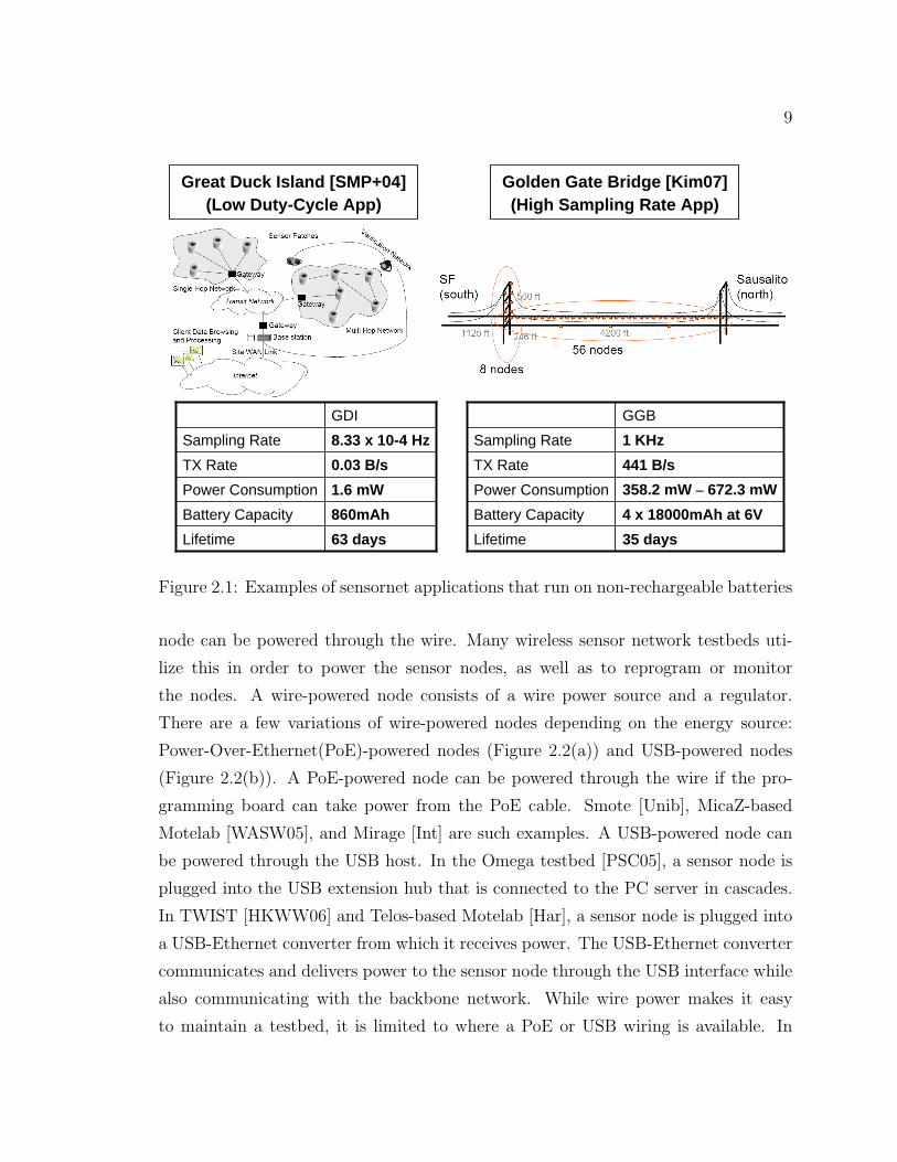
to its limited capacity. Figure 2.1 shows examples of sensornet applications that

run on non-rechargeable batteries. A Great Duck Island node [SMP+04], designed

to monitor the environmental characteristics of a bird’s nest, has a small-capacity

battery so as not to disrupt wildlife. Although sensing and transmission is done at

a low rate, the small battery capacity limits its lifetime to about two months. A

Golden Gate Bridge node [Kim07], is designed to monitor structural health data of

a bridge using time-synchronized high frequency sampling of accelerometer signals.

Even though a Golden Gate Bridge node has the freedom to use a larger battery,

high power consumption of the accelerometer limits its lifetime to a little over one

month. This limited lifetime of a non-rechargeable battery-based node motivates us

to consider other types of energy sources for wireless sensor networks.

2.1.2 Wire-powered Nodes

Another way to supply energy to sensor nodes is through a wired back-channel.

While wireless sensor networks were originally envisioned to be wire-free, a wired

back-channel can be used for maintenance purposes, such as reprogramming and

data downloading. A side effect of using a wired back-channel is that the sensor

9

1.6 mWPower Consumption0.03 B/sTX Rate8.33 x 10-4 HzSampling Rate

860mAhBattery Capacity63 daysLifetime

GDI

Great Duck Island [SMP+04] (Low Duty-Cycle App)

Golden Gate Bridge [Kim07](High Sampling Rate App)

358.2 mW – 672.3 mWPower Consumption441 B/sTX Rate1 KHzSampling Rate

4 x 18000mAh at 6VBattery Capacity35 days

GGB

Lifetime

Figure 2.1: Examples of sensornet applications that run on non-rechargeable batteries

node can be powered through the wire. Many wireless sensor network testbeds uti-

lize this in order to power the sensor nodes, as well as to reprogram or monitor

the nodes. A wire-powered node consists of a wire power source and a regulator.

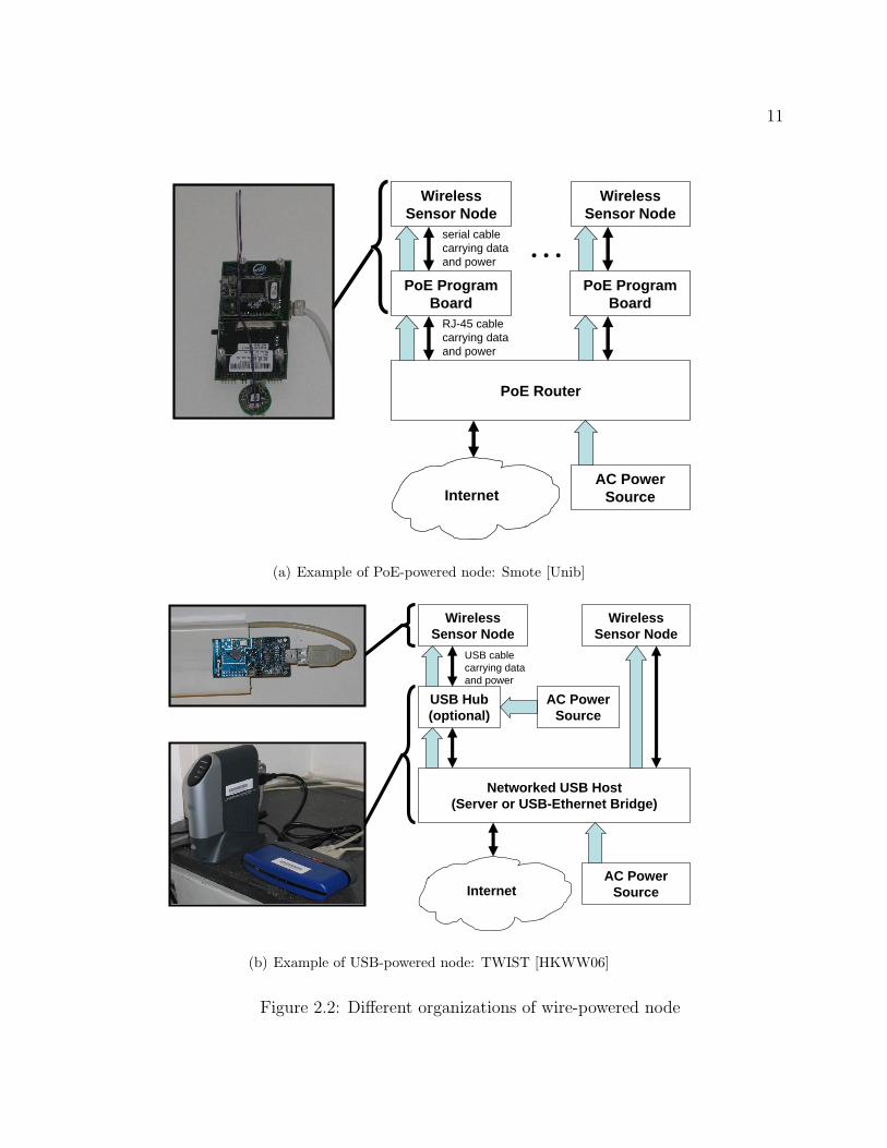
There are a few variations of wire-powered nodes depending on the energy source:

Power-Over-Ethernet(PoE)-powered nodes (Figure 2.2(a)) and USB-powered nodes

(Figure 2.2(b)). A PoE-powered node can be powered through the wire if the pro-

gramming board can take power from the PoE cable. Smote [Unib], MicaZ-based

Motelab [WASW05], and Mirage [Int] are such examples. A USB-powered node can

be powered through the USB host. In the Omega testbed [PSC05], a sensor node is

plugged into the USB extension hub that is connected to the PC server in cascades.

In TWIST [HKWW06] and Telos-based Motelab [Har], a sensor node is plugged into

a USB-Ethernet converter from which it receives power. The USB-Ethernet converter

communicates and delivers power to the sensor node through the USB interface while

also communicating with the backbone network. While wire power makes it easy

to maintain a testbed, it is limited to where a PoE or USB wiring is available. In

10

an outdoor deployment, wire power may not be available, and making such devices

weather-proof or wildlife-safe can add huge cost and complexity. It is the limiter in

outdoor testbeds.

2.1.3 Renewable Energy Sources

A renewable energy-powered node runs on a renewable energy source such as

solar radiation, vibrations, human power, or air flow, and is expected to run for a

long period of time without requiring the replacement of the battery. Typically, a

renewable energy-powered node consists of an energy source, energy collector, energy

storage and regulator. The energy from the energy source is converted into electric

energy through the energy collector, such as a solar cell, piezo electric material or wind

generator. Then, the electric energy generated from the energy collector is stored in

the energy storage, which stores energy and services the load even when the energy

generation rate does not match the energy consumption rate. A regulator can be

used to match the operating range between each component of the power subsystem.

Among the various renewable energy sources, we focus on outdoor solar energy

in this dissertation for two reasons. First, outdoor solar energy has higher power-

density than other renewable energy sources, and this allows us to build a solar-energy

harvesting system with a small form factor (Figure 2.3). Second, the commercial

availability of solar panels allows us to focus on the energy harvesting system from the

perspective of computer science, which consists of synthesis, modeling and analysis,

without the need to build the energy harvesting material itself.

Solar Energy Harvesting

Solar energy harvesting converts solar radiation (energy source) into electric en-

ergy using the photovoltaic effect (energy collector). A few types of semiconductors,

such as polycrystalline silicon can emit electrons when hit by photons. A single solar-

cell outputs voltage between 0.5V and 0.7V, depending on the material, and the

current from the solar-cell is approximately proportional to the area of the solar-cell.

Since the voltage and the current of a single solar-cell may not be large enough to

meet the requirements of the energy consuming device, multiple solar cells are com-

11

PoE Router

PoE ProgramBoard

WirelessSensor Node

AC PowerSource

PoE ProgramBoard

WirelessSensor Node

RJ-45 cablecarrying dataand power

…

Internet

serial cablecarrying dataand power

(a) Example of PoE-powered node: Smote [Unib]

Networked USB Host(Server or USB-Ethernet Bridge)

WirelessSensor Node

AC PowerSource

USB Hub(optional)

WirelessSensor Node

USB cablecarrying dataand power

Internet

AC PowerSource

(b) Example of USB-powered node: TWIST [HKWW06]

Figure 2.2: Different organizations of wire-powered node

12

Outdoor Solar Source by

Sikka et al [SCV+06]

Indoor SolarSource by

Roundy et al [ROC+03]

Human PowerSource by Paradiso

[Paradiso06]

Air FlowSource by

Park et al [Park06]

VibrationsSource by

Roundy et al [ROC+03]

Energy Example Power Size PowerSource DensityOutdoor Fleck node 135.6 mW 115mm x 85mm 1390 uW/cm2

Solar [SCV+06] daily average solar panel(= 11715 J per day)

Indoor RF-TX 2.9 mW 24mm x 33mm 366 uW/cm2

Solar beacon (8 inch under lamp) solar panel[ROC+03] 0.042 mW 5.30 uW/cm2

(ambient office light)Vibrations Piezo- 180 uW volume 1 cm3 180 uW/cm3

electric length 3 cmcollector[Rou03]

Human Piezo- 10 mW 5cm x 5cm 148 uW/cm2

Power electric PZT strip withshoe 5cmx8.5cm sheet[Par06] of spring steel

Wind AmbiMax 47.25 mW Wind generator of[PC06] (wind speed 8.3m/s) 500mW-200rpm

Figure 2.3: Comparison of renewable energy sources

13

monly combined, in a series or parallel, into an array that is able to provide suitable

voltage and current. Such a solar-cell array is called as solar panel.

Vibration

Solar energy has big advantages in the outdoors; it is available in most outdoor

locations and has high power-density. However, it is not very useful in an indoor

environment due to its low power-density. Figure 2.3 shows that the power-density

of indoor light is three orders of magnitude smaller than that of outdoor sunlight;

thus, other energy sources are more suitable depending on the situation. Vibrations

can be a good source of energy when there is a source of continuous vibrations, such

as frequently trodden doormats, motors in industrial facilities and washing machines

are such examples. Roundy demonstrated that a piezoelectric material-based energy

collector can generate 180uW of power [Rou03,RSF+04].

Human Power

Paradiso [Par06] discusses several techniques for harvesting energy from human

activity, such as push-button RF transmitter, magnetic generator based shoe, piezo-

electric based shoe, and parasitic mobility node. For example, a piezoelectric-based

shoe collects 10mW of power. Human power has one advantage over other renewable

energy sources: a small amount of energy can be generated quickly on demand by

a human without depending on the environment. However, it is not suitable as a

steady long-term energy source because intentional use of human power can disrupt

normal human activity.

Wind or Air Flow

Park et al. demonstrated that a mote-scale device (AmbiMax node) can operate

on wind-generated power [PC06]. The AmbiMax node stores the energy from a wind

generator 1 in a supercapacitor and performs maximum power point tracking (MPPT)

between the wind generator and the supercapacitor. However, wind power has some

drawbacks. Compared to solar power, its energy density is smaller (380µW/cm3 vs.

1AmbiMax used a wind generator that outputs 1W at 2000rpm and 0.25W at 1000rpm.

14

External Environment

SolarPanel

InputRegulator

EnergyStorage

LoadOutputRegulator

Sun

Figure 2.4: A general model for micro-solar power system

15000µW/cm3 [RSF+04]), and the available hours of wind power are shorter than

those of solar power [PC06].

2.2 Prior Work on Micro-solar Power Systems

Typically, as shown in Figure 2.4, a micro-solar power system has the following

organization: (a) an external environment that determines the amount of solar radi-

ation available to the micro-solar power system, (b) a solar panel that collects solar

energy, (c) energy storage, where extra energy from the solar panel is stored, (d) a

load that will run on top of the power subsystem, consuming energy from the solar

panel and the energy storage, (e) an input regulator that maximizes input power by

matching the operating point between the solar panel and the energy storage, and (f)

an output regulator that regulates the output voltage of the energy storage.

In this section, we develop a taxonomy of micro-solar power subsystems based

on previously published systems, and we discuss strengths and weaknesses of each

micro-solar power system design. From this, we distill a few designs of micro-solar

power systems that are representative of different design points and have reasonable

performance metrics.

15

2.2.1 Micro-solar Power System Platforms

Categorized by Storage and Charging Management

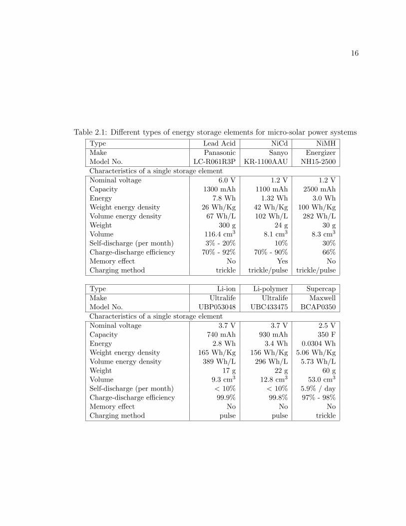
First, we can categorize micro-solar power systems depending on the type of energy

storage and its charging management. Table 2.1 lists lead acid battery, NiCd battery,

NiMH battery, Li-ion battery, Li-polymer battery, and supercapacitor as energy storage

for micro-solar power systems.

The Lead acid battery is the most commonly used energy storage in macro-solar

power systems because it is easy to make in a large capacity, it can provide current

high enough to drive residential electric devices, and its charging method is simple.

But, at the scale of micro-solar power systems, it is not preferred due to its smaller

energy density.

The NiMH battery is one of the most popular types of energy storage for micro-

solar power systems. This is because it has relatively high energy density, its charging

method is simple, it is relatively inexpensive, and it can be replaced with a non-

rechargeable battery when it is not charged. Among the micro-solar power systems

we reviewed, Heliomote [RKH+05], Fleck [CVS+07] and HydroWatch [TJC08] used

a NiMH battery as their energy storage. Since the current from the solar panel is

relatively small compared to the maximum charging current, these platforms employ

trickle charging, which can be done with a simple hardware-based controller.

The NiCd battery is similar to NiMH in a few cases: it has similar charging and

discharging characteristics and it is available in standard battery form factors (e.g.

AA, AAA, C) just as is the NiMH battery. This means that NiMH and NiCd are

interchangeable in most cases. The differences are that the capacity of NiCd is smaller

than NiMH (1100mAh vs. 2500mAh in Table 2.1), it has a memory effect that causes

its capacity to decrease over multiple uses, and it contains cadmium that can be

harmful when exposed to the environment. For this reason, NiMH is preferred over

NiCd for micro-solar power systems.

The Li-ion (or Li-polymer) battery has the highest energy density and a high

charge-to-discharge efficiency. This makes the Li-ion battery a good candidate for

energy storage when the micro-solar power system needs a small form factor. However,

the charging mechanism of a Li-ion battery is more complicated than that of other

16

Table 2.1: Different types of energy storage elements for micro-solar power systems

Type Lead Acid NiCd NiMHMake Panasonic Sanyo EnergizerModel No. LC-R061R3P KR-1100AAU NH15-2500Characteristics of a single storage elementNominal voltage 6.0 V 1.2 V 1.2 VCapacity 1300 mAh 1100 mAh 2500 mAhEnergy 7.8 Wh 1.32 Wh 3.0 WhWeight energy density 26 Wh/Kg 42 Wh/Kg 100 Wh/KgVolume energy density 67 Wh/L 102 Wh/L 282 Wh/LWeight 300 g 24 g 30 gVolume 116.4 cm3 8.1 cm3 8.3 cm3

Self-discharge (per month) 3% - 20% 10% 30%Charge-discharge efficiency 70% - 92% 70% - 90% 66%Memory effect No Yes NoCharging method trickle trickle/pulse trickle/pulse

Type Li-ion Li-polymer SupercapMake Ultralife Ultralife MaxwellModel No. UBP053048 UBC433475 BCAP0350Characteristics of a single storage elementNominal voltage 3.7 V 3.7 V 2.5 VCapacity 740 mAh 930 mAh 350 FEnergy 2.8 Wh 3.4 Wh 0.0304 WhWeight energy density 165 Wh/Kg 156 Wh/Kg 5.06 Wh/KgVolume energy density 389 Wh/L 296 Wh/L 5.73 Wh/LWeight 17 g 22 g 60 gVolume 9.3 cm3 12.8 cm3 53.0 cm3

Self-discharge (per month) < 10% < 10% 5.9% / dayCharge-discharge efficiency 99.9% 99.8% 97% - 98%Memory effect No No NoCharging method pulse pulse trickle

17

types of energy storage. This means that the system with a Li-ion battery needs

either a dedicated charge management chip or software control to correctly control the

battery. Among micro-solar power systems, ZebraNet [ZSLM04], Prometheus [JPC05]

and Trio [DHJ+06] used a Li-ion battery as its energy storage, and it charged the

battery using software control.

A supercapacitor is a capacitor whose capacity is high enough to be used as energy

storage for low-power electronic devices (usually higher than 1F to 10F). While its

capacity is still much smaller than other types of batteries, its very high maximum

recharge cycles allows it to be used for long-lifetime applications. EverLast [SC06]

used a supercapacitor for its energy storage.

Micro-solar power systems such as Prometheus [JPC05], Trio [DHJ+06] and Am-

biMax [PC06] used multiple levels of storage that consist of a supercapacitor and a

Li-ion battery. Such a system can take the benefits of both the supercapacitor and

Li-ion battery: a long lifetime and large capacity with high efficiency. The charging

management is more complicated for a hybrid storage system because it has to choose

which storage to charge and when to charge. While the charging controller can be

made in hardware (AmbiMax), it can also be made in software (Prometheus and Trio)

by using the sensing and actuation capability of a sensor node.

Categorized by Solar-Panel Operation

Since the output power of a solar panel bounds the available energy for a micro-

solar power system, a well-designed system should keep the operating point of the

solar panel closely to the maximum power point so that the maximum output of

power can be transferred from the solar panel. The operating point of the solar panel

is determined by either an input regulator or energy storage depending on whether an

input regulator is present. We can categorize published designs of micro-solar power

systems depending on how the operating point of the solar panel is determined.

First, most NiMH battery-based designs have the solar panel operating point

set to the voltage level of the energy storage (Heliomote [RKH+05], Fleck [CVS+07],

HydroWatch [TJC08]). These designs use the fact that the voltage range of the NiMH

while charging is relatively narrow. They can achieve near-optimal performance by

choosing the solar panel that has its maximum power point in the charging range of

18

the NiMH battery.

Second, the operating point of the solar panel can be set to a fixed range as in

ZebraNet [ZSLM04]. Compared to other micro-solar power systems, ZebraNet uses a

solar panel that has a relatively low open-circuit voltage (1.55V) and this makes the

solar panel operating range for maximum power transfer narrow. ZebraNet sets the

operating point of the solar panel to a fixed range of 1.3V to 1.5V using a comparator

and an input regulator.

Third, the maximum power point tracking should be used for a supercapacitor-

based system. This is because the supercapacitor has a wide operating range and its

energy transfer is not efficient when the operating point of the supercapacitor is far

from the maximum power point of the solar panel. EverLast [SC06] dynamically ad-

justs the operating point of the solar panel by controlling the input regulator through

the micro-controller. In Everlast, the micro-controller periodically reads the open-

circuit voltage of the solar panel by turning off the input regulator, and calculates

the maximum power point of the solar panel based on the open-circuit voltage. Then,

the micro-controller reads the solar panel operating point through an ADC and turns

on or off the input regulator so that the solar panel operating point is maintained

around the maximum power point. AmbiMax [PC06] also dynamically adjusts the

operating point of the solar panel, but it uses the photo sensor and the comparator

to control the input regulator.

Figure 2.5 summarizes the characteristics of several micro-solar power system

platforms.

2.2.2 Micro-solar Power System Models

Adaptive Workload Scheduling

Some of the previous research has shown that duty-cycle [JPC05,RKH+05,KPS04,

KHZS07,VGB07,NLA+07], task scheduling [MBTB06a], or energy harvesting-aware

programming language [SKG+07] could be adjusted dynamically, depending on the

environment, in order to achieve higher utilization and meet the scheduling deadlines.

Jiang et al. [JPC05] showed a simple duty-cycling scheme that changes the duty-

cycle depending on the solar level. However, their work just showed a proof of concept

19


SolarPanel

InputRegulator

Energy Storage

LoadOutputRegulator

Sun

NiMH Battery

System on NiMH battery

Mote

(a) System on NiMH battery


SolarPanel

Input Regulator

Energy Storage

LoadOutputRegulator

Sun

Li-Ion Battery

System on Li-Ion battery

Comparator

Switching Regulator

Mote

(b) System on Li-Ion battery


SolarPanel

Input Regulator

Energy Storage

LoadOutputRegulator

Sun

Li-ion Battery

System on supercapacitor and Li-ion battery with software charging control

Supercap

Mote

Batt Charging

Switch

Storage Selection

Switch

(c) System on supercap and Li-Ion battery


SolarPanel

Input Regulator

Energy Storage

LoadOutputRegulator

Sun

Supercap

System on supercapacitor with software-controlled MPPT

MPPT Controller Mote

(d) System on supercap with SW-controlled

MPPT


SolarPanel

Input Regulator

Energy Storage

LoadOutputRegulator

Sun

Li-ion Battery

System on supercap and Li-ion battery with HW-controlled MPPT and charging

Supercap

MoteMPPT Controller

(e) System on supercap and Li-ion battery with

HW-controlled MPPT

Examples EnergyStorage

Solar Panel OperatingPoint

(a) Heliomote [RKH+05] NiMH Depends on battery voltageFleck [CVS+07]HydroWatch [TJC08]

(b) ZebraNet [ZSLM04] Li-ion Fixed range controlled by com-parator and switching regulator

(c) Prometheus [JPC05] Supercap and Operating range set by softwareTrio [DHJ+06] Li-ion

(d) Everlast [SC06] Supercap MPPT controlled by softwareand switching regulator

(e) AmbiMax [PC06] Supercap andLi-ion

MPPT controlled by compara-tor and switching regulator

Figure 2.5: Comparison of micro-solar power system platforms

20

without formulating the relation between the desired duty-cycle rate and the corre-

sponding system parameters. Moser et al. [MBTB06b] showed an algorithm that

schedules tasks to meet deadlines within the constraint of varying energy supply and

storage. However, their algorithm has drawbacks in that it assumes non-ideal per-

fect storage (no leakage and non-ideal storage round-trip efficiency) and the results

were shown only in simulation, with no consideration of realistic energy harvesting

devices. Kansal et al. [KPS04] showed a bound rule for sustainable operation of

energy-harvested nodes. They demonstrated the sustainable operation of a single

node using Heliomote by setting its parameters according to the bound rule. But,

in the case of multiple nodes, they just showed the concept without demonstration.

Kansal et al. [KHZS07] proposed an adaptive duty-cycling that tries to achieve max-

imum utility of an energy harvesting system, and showed that their algorithm had

its energy utilization very close to the optimum value that could be achieved with

complete knowledge of energy supply and consumption in the future. This paper

demonstrated adaptive duty-cycling using two example cases (field monitoring and

event monitoring).

Simulating Power Consumption of Load

There are several sensor network simulators that can estimate power consump-

tion of sensor nodes. PowerTOSSIM [SHC+04], SensorSim [PSS00, PSS01], Prowler

[SVML03], SENS [SKA04] and AEON [LWG05] are such examples. These simula-

tors are similar to each other in that they execute a sensor network application and

estimate power consumption based on the pre-recorded energy consumption profile

of primitive operations on the target sensor node platform. On the other hand, they

differ in simulation platform, target sensor node platform, source base and extensi-

bility. The characteristics of some sensor network power simulators are summarized

in Table 2.2.

When we choose a sensor network power simulator, we are interested in two factors:

reality and extensibility. The result from a simulator wouldn’t be meaningful if the

simulator did not reflect real sensor networks. In this sense, we prefer a simulator

that takes an actual application program code and simulates the corresponding power

consumption. PowerTOSSIM [SHC+04] and AEON [LWG05] are such examples.

21

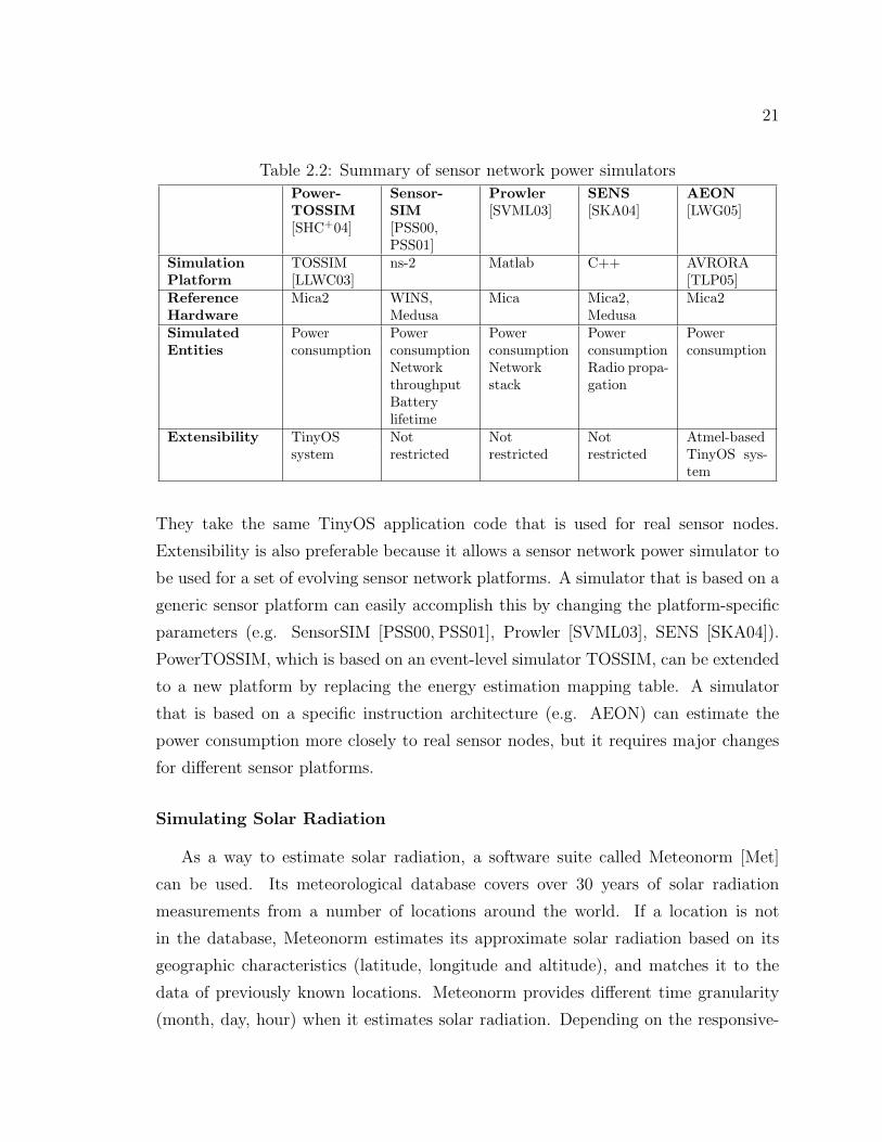
Table 2.2: Summary of sensor network power simulators

Power-TOSSIM[SHC+04]

Sensor-SIM[PSS00,PSS01]

Prowler[SVML03]

SENS[SKA04]

AEON[LWG05]

SimulationPlatform

TOSSIM[LLWC03]

ns-2 Matlab C++ AVRORA[TLP05]

ReferenceHardware

Mica2 WINS,Medusa

Mica Mica2,Medusa

Mica2

Simulated Power Power Power Power PowerEntities consumption consumption consumption consumption consumption

NetworkthroughputBatterylifetime

Networkstack

Radio propa-gation

Extensibility TinyOS Not Not Not Atmel-basedsystem restricted restricted restricted TinyOS sys-

tem

They take the same TinyOS application code that is used for real sensor nodes.

Extensibility is also preferable because it allows a sensor network power simulator to

be used for a set of evolving sensor network platforms. A simulator that is based on a

generic sensor platform can easily accomplish this by changing the platform-specific

parameters (e.g. SensorSIM [PSS00, PSS01], Prowler [SVML03], SENS [SKA04]).

PowerTOSSIM, which is based on an event-level simulator TOSSIM, can be extended

to a new platform by replacing the energy estimation mapping table. A simulator

that is based on a specific instruction architecture (e.g. AEON) can estimate the

power consumption more closely to real sensor nodes, but it requires major changes

for different sensor platforms.

Simulating Solar Radiation

As a way to estimate solar radiation, a software suite called Meteonorm [Met]

can be used. Its meteorological database covers over 30 years of solar radiation

measurements from a number of locations around the world. If a location is not

in the database, Meteonorm estimates its approximate solar radiation based on its

geographic characteristics (latitude, longitude and altitude), and matches it to the

data of previously known locations. Meteonorm provides different time granularity

(month, day, hour) when it estimates solar radiation. Depending on the responsive-

22

ness of the application, solar radiation estimates of suitable time granularity can be

used.

With an astronomical model, we estimate the solar radiation using parameters

that affect the angle between the sunlight and the solar panel. When the angle of

sunlight from the normal to the solar panel is Θ, the effective sunlight that shines on

the solar panel is proportional to cos Θ [DHM75]. The angle Θ depends on solar-panel

inclination θp, panel orientation φp, latitude L, time of the day t, and day of the year

n.

Simulating the Battery

A couple of research groups proposed a way to estimate the battery capacity

or lifetime for WSNs [PSS00, PSS01, VXSB07]. Although these are built to model

the discharge rate of a non-rechargeable battery, they can be extended for micro-

solar power systems by considering the charging profile of the battery as well as the

discharging profile. These battery simulators vary in terms of their functions and

complexity.

SensorSim by Park et al. [PSS00], which is a network-level simulator of a WSN,

can also simulate energy-related metrics such as the capacity of a battery. It simulates

the capacity of a battery using a linear model, which means the amount of energy

that is drawn from the battery is proportional to the total aggregate power of a

sensor node. SensorSim was extended to reflect different types of battery models in

the follow-on paper [PSS01]: a linear model, a discharge rate-dependent model and

a relaxation model. With the discharge-rate-dependent model, the battery capacity

depends not only on the time duration, but also on the discharge rate. With this

model, the charge the battery can drive is close to the initial charge at low current

draw, and it becomes smaller as the current draw becomes higher. The extended

version of SensorSim also reflects the relaxation model. With the relaxation model,

the battery capacity decreases sharply under a heavy load, but recovers if the current

draw becomes low again. sQualNet [VXSB07] by Varshney et al. is another network-

level simulator for WSN. sQualNet proposes two techniques for modeling battery

capacity. First, they propose using polynomial functions to calculate the battery

capacity. Second, they propose using a small recent history, rather than the entire

23

Adaptive Workload Scheduling

Duty-Cycling[JPC05, KPS04, KHZS07]

Task-Schduing[MBTB06a]

Power ConsumptionSimulation

PowerTOSSIM [SHC+04]SensorSim [PSS00,PSS01]

Prowler [SVML03]SENS [SKA04]AEON [LWG05]

Solar RadiationSimulation

Meteonorm [Met]

Dave et al. [DHM75]

BatterySimulation

SensorSim [PSS00,PSS01]

sQualNet [VXSB07]


SolarPanel

InputRegulator

EnergyStorage

LoadOutputRegulator

Sun

Figure 2.6: Previous works on micro-solar power system models

battery history. This reduces the memory requirements.

Figure 2.6 summarizes previous works on micro-solar power system models in

relation to the general model of micro-solar power systems.

2.2.3 Relation to Macro-Solar Power Systems

We can categorize the solar energy harvesting systems by the output power of

the solar panel. Macro-solar and meso-solar power systems are commercial and

residential solar energy harvesting installations, and use a scale of kilowatts and

watts. A micro-solar power system, however, is a small, low-power electronics with

a solar panel of less than 1 Watt of power. Macro-solar and meso-solar systems have

the same basic component categories and the same interconnection as a micro-solar

power system. The difference is the relative sizes, which translates into differences in

the design and deployment of a micro-solar power system. First, with a micro-solar

power system, the load is on the same scale as the management of the system, and the

system as a whole has to be very efficient and well-matched. Second, with a micro-

solar power system, the device is located where the measurement must be taken, not

where the sun is best. Thus, a micro-solar power system should be planned for the

24

environment that exists, rather than be planned for the environment that is desired.

There are many calculators for macro-solar power systems [Nat,fin,Iow,Sun,Cal,Wea].

Concepts from these tools can be applied to micro-solar power systems: they compose

a system as a collection of several components and their interconnections; and they

estimate solar radiation using an astronomical model. However, they are not suitable

for modeling the dynamics of micro-solar power systems due to the following reasons.

First, each component is represented as a single number rather than a function or a

curve. This approach may predict the average or maximum performance, but cannot

predict the varying performance with different operating points. Second, due to

economic reasons, these macro-solar tools assume that energy surpluses are sold to

the grid rather than accumulated into energy storage. However, because micro-solar

power systems are often placed where grid power is not available, micro-solar systems

generally require energy storage, breaking the assumption used in these macro-solar

tools.

2.3 Refined Problem Statement

As stated in the previous chapter, building a micro-solar power system has four

main challenges: large design space, long time-scale, different environments for de-

velopment and deployment sites, and variability of solar energy. In this dissertation,

we provide a practical theory of micro-solar power systems to address these problems

and guide specific design choices. It presents a general architecture of micro-solar

power systems describing key components and interconnections among the compo-

nents, and it formalizes each component of the architecture in either an analytical or

empirical model of its behavior. Finally, it incorporates these component models and

their interconnections in a simulation suite.

We take a modular approach to modeling micro-solar power systems over a large

design space. As shown in Figure 2.7, a micro-solar power system consists of the six

components – external environment, solar panel, energy storage, load, input regulator

and output regulator – and its design space is a cross-product of all the possible

choices for its components. In order to abstract such a large diversity in a single

framework, the simulation suite represents each component of a micro-solar power

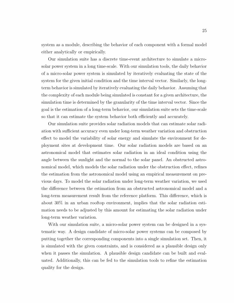
25

system as a module, describing the behavior of each component with a formal model

either analytically or empirically.

Our simulation suite has a discrete time-event architecture to simulate a micro-

solar power system in a long time-scale. With our simulation tools, the daily behavior

of a micro-solar power system is simulated by iteratively evaluating the state of the

system for the given initial condition and the time interval vector. Similarly, the long-

term behavior is simulated by iteratively evaluating the daily behavior. Assuming that

the complexity of each module being simulated is constant for a given architecture, the

simulation time is determined by the granularity of the time interval vector. Since the

goal is the estimation of a long-term behavior, our simulation suite sets the time-scale

so that it can estimate the system behavior both efficiently and accurately.

Our simulation suite provides solar radiation models that can estimate solar radi-

ation with sufficient accuracy even under long-term weather variation and obstruction

effect to model the variability of solar energy and simulate the environment for de-

ployment sites at development time. Our solar radiation models are based on an

astronomical model that estimates solar radiation in an ideal condition using the

angle between the sunlight and the normal to the solar panel. An obstructed astro-

nomical model, which models the solar radiation under the obstruction effect, refines

the estimation from the astronomical model using an empirical measurement on pre-

vious days. To model the solar radiation under long-term weather variation, we used

the difference between the estimation from an obstructed astronomical model and a

long-term measurement result from the reference platform. This difference, which is

about 30% in an urban rooftop environment, implies that the solar radiation esti-

mation needs to be adjusted by this amount for estimating the solar radiation under

long-term weather variation.

With our simulation suite, a micro-solar power system can be designed in a sys-

tematic way. A design candidate of micro-solar power systems can be composed by

putting together the corresponding components into a single simulation set. Then, it

is simulated with the given constraints, and is considered as a plausible design only

when it passes the simulation. A plausible design candidate can be built and eval-

uated. Additionally, this can be fed to the simulation tools to refine the estimation

quality for the design.

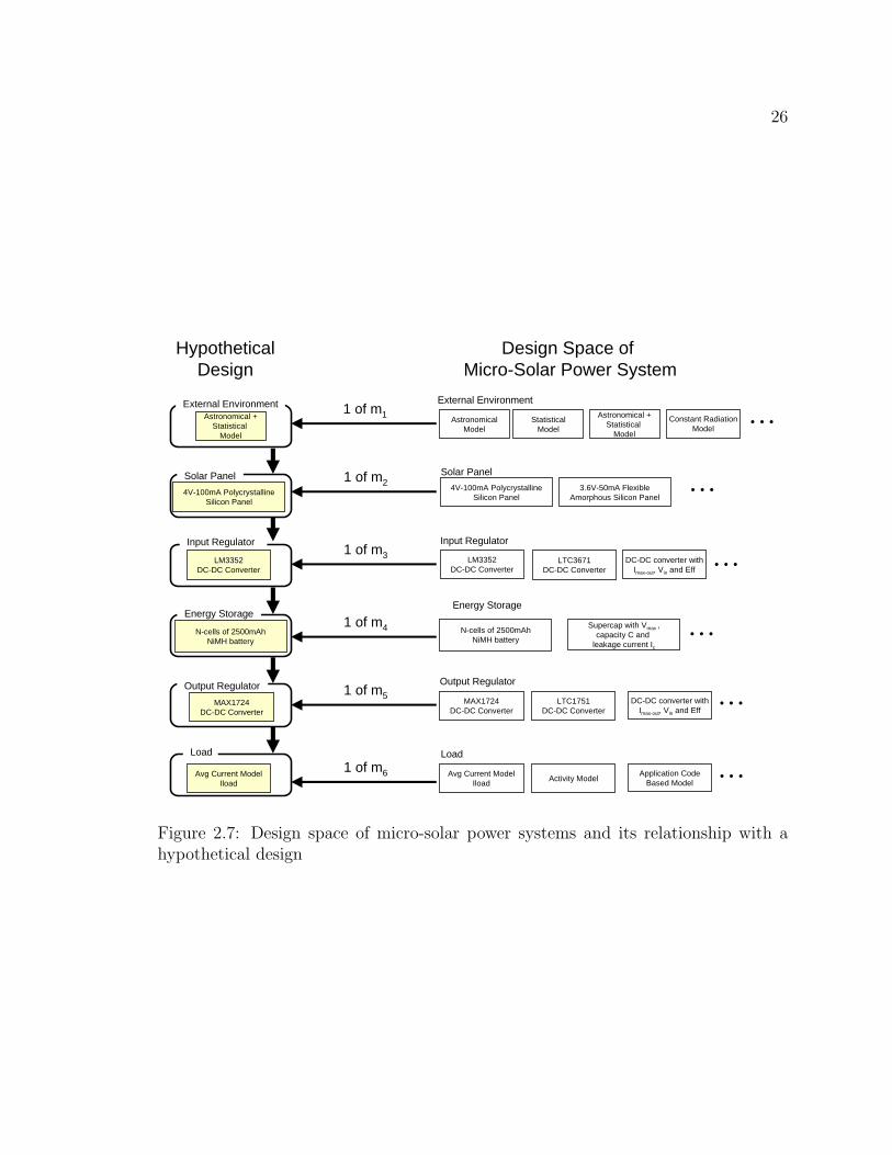
26

Energy Storage

Output Regulator

Input Regulator

Load

Solar Panel


Supercap with Vmax ,capacity C and

leakage current Ic

Energy Storage

N-cells of 2500mAhNiMH battery

…

LTC1751DC-DC Converter

Output Regulator

MAX1724DC-DC Converter

…DC-DC converter withImax-out, Vin and Eff


Input Regulator

LM3352DC-DC Converter


Activity Model

Load

Avg Current ModelIload

…Application CodeBased Model

3.6V-50mA FlexibleAmorphous Silicon Panel

Solar Panel4V-100mA Polycrystalline

Silicon Panel…


AstronomicalModel

…StatisticalModel

Astronomical +Statistical

Model

Constant RadiationModel

4V-100mA PolycrystallineSilicon Panel



Astronomical +Statistical

Model



HypotheticalDesign

Design Space of Micro-Solar Power System

1 of m1

1 of m2

1 of m3

1 of m4

1 of m5

1 of m6

Figure 2.7: Design space of micro-solar power systems and its relationship with ahypothetical design

27

Chapter 3

Architecture of Micro-solar Power

Systems

This chapter presents an architecture of micro-solar power systems describing the

characteristics of its key components and the relationships among the components.

Then, it provides an empirical analysis of two well-studied designs as concrete exam-

ples of micro-solar power systems, and finally it summarizes the proposed architecture.

3.1 Overall Architecture of Micro-solar Power Sys-

tems

In general, any solar-powered system consists of the following six components:

external environment, solar panel, input regulator, energy storage, output regulator

and load (Figure 3.1). The solar energy from the environment is collected by the

solar collector and is made available for the operation of the load. The energy storage

is used to buffer the varying energy income and distribute it to the load throughout

the duration. The input regulator can be used to adjust the mismatch between the

operating range of the solar panel and the energy storage, while the output regulator

is used to shape the operating range of the energy storage to that of the load. The

design decisions for each component will dictate the energy flow between them and

the overall behavior of the system.

In the rest of this chapter, we describe the architecture of a micro-solar power

28

Figure 3.1: Model for a solar-powered sensor system

Table 3.1: Evaluation metrics

Metric DescriptionPsolar−in Total incident solar radiation.Psol Power produced by the solar panel.Pstorage−in Power collected by the solar-collector.Pbat−chg Power stored in the energy storage.Pbat−dis Power extracted from the energy storage.Pmote Energy consumed by the mote.Effreg−in Efficiency of the input regulator.Effreg−out Efficiency of the output regulator.

system in terms of the energy flow of each component. Section 3.1.1 shows how

to estimate solar radiation (Psolar−in) using statistical and mathematical methods.

Section 3.1.2 discusses the factors that affect the solar panel operating point (Psol).

Section 3.1.3 discusses the effect of input-power conditioning (Effreg−in). Section 3.1.4

discusses the factors that affects the storage capacity and the lifetime. Section 3.1.5

discusses the effect of output-power conditioning (Effreg−out). Section 3.1.6 explains

how to model the energy consumption of a mote (Pcons) with radio duty-cycling.

Table 3.1 lists the metrics that will be used throughout this chapter.

29

North

Zenith Normal tothe surface

Sun

East

Projections

Surface

Figure 3.2: Definition of the angles used in astronomical method – courtesy of Daveet al.

3.1.1 External Environment

The amount of solar radiation Psolar−in depends on the environment, and places an

upper bound on the maximum energy output of the solar collector Psol. Most previous

designs of micro-solar power sensor systems did not carefully model solar radiation:

they either paid little attention to the available solar energy or considered a constant

average solar radiation [ROC+03, SC06, JPC05, DHJ+06, SCV+06, RKH+05]. Kansal

et al. [KPS04] proposed a rule for perpetual operation, which stated a relationship

between the node consumption and the energy budget. However, this rule considered

a generic energy input and did not provide a way to estimate the energy budget for

solar energy harvesting. In this dissertation, we describe three ways to estimate solar

radiation: (a) an astronomical method, (b) an astronomical method with history of

weather effects, (c) an astronomical method with local enhancements.

With an astronomical model, we estimate the solar radiation using the parameters

that affect the angle between the sunlight and the solar panel. According to Dave

30

et al. [DHM75] (Figure 3.2), the effective sunlight that shines on the solar panel is

proportional to cos Θ when the angle of sunlight from the normal to the solar panel is

Θ, The angle Θ depends on solar panel inclination θp, panel orientation φp, latitude

L, time of the day t, and day of the year n:

cos Θ = cos θp · cos θs + sin θp · sin θs · cos(φp − φs) (3.1)

cos θs = sin δ · sinL+ cos δ · cosL · cosh

sinφs = − cos δ · sinh/ sin θs

x = 2πn/365

h = 15(t− 12)

δ = 0.302− 22.93 cosx− 0.229 cos 2x− 0.243 cos 3x

+ 3.851 sinx+ 0.002 sin 2x− 0.055 sin 3x

With an astronomical method with history of weather effects, we estimate the solar

radiation under the influence of weather effects by using the history of solar radiation

measurements. In order to get such a history, we can use a meteorological database

software suite such as Meteonorm [Met], which estimates solar energy radiation as a

monthly solar radiation Emonth (kWh/m2). Using Emonth, we can calculate the peak

solar hours (PSH), which is the equivalent number of solar radiation hours per day

assuming that the same amount of solar energy is given at an uniform intensity of

1kW/m2. Then, the available energy from a specific solar panel for one day, Esol−day,

can be estimated as the product of the PSH and the solar panel output power Ppanel

at 1kW/m2 (usually provided by its manufacturer):

Esol−day = PSH · Ppanel =Emonth · Ppanel

1kW/m2 ·#days(3.2)

As well as the weather effects, occlusions from local objects such as trees and

buildings can affect solar radiation. With an astronomical method with local en-

hancements, we refine the solar radiation estimate from the astronomical method

with a measurement of local obstructions.

31

0 2 4 6 80

10

20

30

40

Solar Panel Voltage (V)

So

lar

Pan

el C

urr

ent

(mA

)Trio Solar−Panel I−V Curve

6/30/2006 3:52pmMax Power Point

Isc

Voc

(VmaxP , ImaxP )

0 2 4 6 80

50

100

150

200


So

lar

Pan

el P

ow

er (

mW

)

Trio Solar−Panel Output Power

6/30/2006 3:52pmMax Power Point (VmaxP , PmaxP )

Figure 3.3: Characteristics of a solar panel: (a) I-V curve, (b) P-V curve with MPP

3.1.2 Solar Collector

Solar energy from the environment is converted to electric energy by the solar

collector, which includes a solar panel and a regulator. The solar panel converts

photons into electricity and the regulator conditions the output power of the solar

panel for energy transfer to the storage. The amount of solar power out of the solar

collector Psol is determined by the following factors: (1) solar radiation, (2) solar-panel

characteristics, (3) the operating point of the solar-panel.

The solar panel I-V curve describes how the output current of a solar panel behaves

at a certain radiation condition. (Figure 3.3). The current of a solar panel is at a

maximum when the impedance across the two terminals of the solar panel is zero,

and the current at the zero impedance is called the short circuit current (Isc). As

the impedance increases, the current from the solar panel decreases and the voltage

across the two terminals of the solar panel increases. When the impedance becomes

infinite, the current becomes zero. The solar panel voltage at this point is called

the open circuit voltage (Voc). In order to deliver the highest power from the solar

panel, we need to operate the solar panel near the optimum point. This optimum

point (VmaxP , ImaxP ) is called the maximum power point (MPP), and the power at

the maximum power point is no less than the power at any other points (V , I):

VmaxP · ImaxP ≥ V · I for any (V ,I) (3.3)

32

The solar-panel I-V characteristic also depends on the radiation condition. As the

solar irradiance increases or decreases, the I-V curve moves outwards or inwards.

Thus, a solar panel can be described as a sequence of I-V curves with each I-V curve

corresponding to a particular solar irradiance condition. Figure 3.4 shows I-V curves

for a solar panel at different times of day. Each I-V curve in Figure 3.4 is drawn

by fitting an exponential curve to 20 sample points. We notice that some of the I-V

curves are non-monotonic even though they are not expected to overlap. This is an

artifact of sampling errors and curve fitting. The current of an I-V curve around

the open-circuit voltage is much lower than the peak value and even a small amount

of sampling error in the open-circuit voltage region can change the shape of an I-V

curve.

In order to maximize the power transfer from the solar panel, it is recommended

that the regulating circuit operate near the maximum power point (MPP), which is

the point in the I-V curve where P = I · V is maximized. As a way of achieving

maximum power transfer, a maximum power point tracker can be used (e.g. Everlast

[SC06]). An active circuit is usually required when the energy signal is near DC.

While this may sound like an attractive option, care needs to be taken when using

it in practice. Since the power a sensor node operates at is usually very small (in

the mW range), the energy consumed by the maximum power point tracker becomes

significant, and sometimes more than what it can save. Figure 3.5 compares the solar

panel output power of the Trio node at its operating point with the output power

that would have been achieved with the maximum power point tracking. Notice that

at the end of day, the daily cumulative solar radiation for each case is 2,666J and

3,055J. The difference, 389J, is 13% of the daily solar radiation at the MPP. Using

a maximum power point tracker is meaningful when its daily energy consumption is

smaller than this.

3.1.3 Input-power Conditioning

In a micro-solar power system, an input regulator can be used to set the specific

operating point of the solar panel to meet the operational constraints of the partic-

ular energy storage using voltage limits, current limits, and charge duration. While

matching the operating points of the solar panel and the energy storage is an advan-

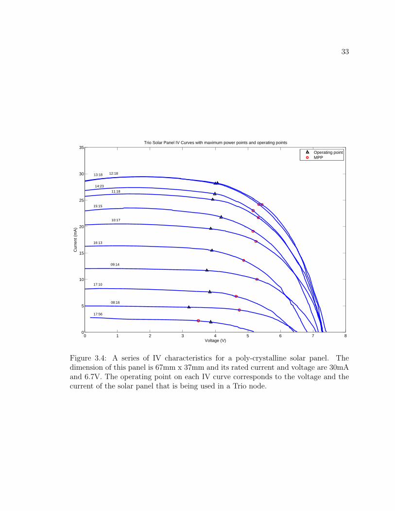
33

0 1 2 3 4 5 6 7 80

5

10

15

20

25

30

35

Voltage (V)

Cur

rent

(m

A)

Trio Solar Panel IV Curves with maximum power points and operating points

Operating pointMPP

17:56

08:16

17:10

09:14

16:13

10:17

15:15

11:18

14:23

13:18 12:18

Figure 3.4: A series of IV characteristics for a poly-crystalline solar panel. Thedimension of this panel is 67mm x 37mm and its rated current and voltage are 30mAand 6.7V. The operating point on each IV curve corresponds to the voltage and thecurrent of the solar panel that is being used in a Trio node.

34

06:00 09:00 12:00 15:00 18:00 21:000

50

100

150

Time

Pow

er (

mW

)

Comparison of solar panel output power: operating point vs MPP

Operating pointMPP

06:00 09:00 12:00 15:00 18:00 21:000

500

1000

1500

2000

2500

3000

3500

Time

Ene

rgy

(J)

Comparison of daily cumulative solar radiation: operating point vs MPP

Operating pointMPP

Figure 3.5: Comparison of solar panel output power and cumulative solar radiationfor solar panel at operating point and MPP with a Trio node.

35

tage of using an input regulator, the sub-unity efficiency of the input regulator is a

drawback. The efficiency of an input regulator, Effreg−in, is 50% to 80% depending

on the part being used. Thus, the analysis of the possible gain of the operating point

matching against the inefficiency of the input regulator should be made before it is

used in a micro-solar power system.

3.1.4 Energy Storage

Energy storage is the group of storage elements used to buffer the energy coming

from the solar collector and to deliver it to the mote in a predictable fashion. Energy

storage can consist of any number of storage elements grouped together in some

configuration. The challenge is to find a desirable configuration and combination of

storage elements so that the requirements are met.

In general, designing the energy storage involves choosing the storage elements

and charging mechanism for correct operation and efficient energy transfer. As a

first step of storage design, a system designer should consider system requirements as

follows:

• Lifetime: The lifetime of the energy storage is determined by the maximum

charge or discharge cycles and depth of discharge. The lifetime should be long

enough to avoid frequent replacement.

• Capacity: The energy storage should be large enough to support the opera-

tion of the end device under the disruption of solar energy. The capacity of the

storage should be proportional to the blackout period that the storage is desired

to support. It is important to realize that the energy input is not a constant,

and therefore the buffers need to be sized appropriately to accommodate envi-

ronmental variations. Other than nominal capacity of the storage element, self

discharge rate and memory effects also affect the storage capacity. The effective

storage capacity should be corrected for these factors:

• Current draw: The energy storage should also be able to support a short

burst of power (the maximum current draw of the end device).

36

• Size and weight: A system designer should pick energy storage elements that

meet the requirement of the application.

Table 2.1 in Section 2.2.1 lists the characteristics of different storage elements. For

micro-solar power systems, a NiMH battery, Li-ion / Li-polymer or supercapacitor

is desirable. The NiCd battery is not preferred due to its smaller energy density,

memory effects and harmful environmental effects. Depending on the priority of

requirements: NiMH battery (capacity and cost), Li-ion / Li-polymer (high energy

density and capacity), or supercapacitor (lifetime) can be chosen.

Configuring the connection between the power supply and the energy storage, and

the connection between the energy storage and the mote presents another opportunity

for system optimization. More importantly, different configurations of energy storage

elements allow greater freedom in how to best satisfy the various requirements stated

above. Compared to using a single type of storage element, a combination of stor-

age elements with different capacities has a desirable characteristic: short, frequent

disruptions are buffered by a smaller capacity storage, while larger but less frequent

disruptions are buffered by a larger capacity storage. In this way, small disruptions do

not affect the lifetime of a larger storage element, which may often have fewer charge

cycles. A side effect of two-level storage is additional energy loss caused by sub-unity

round-trip efficiency of an energy storage element, so the charging mechanism should

be designed to minimize this.

The charging mechanism is another factor that affects system performance. De-

pending on the decisions in the charging mechanism (e.g. when and how much), the

amount of energy that can be transferred to the storage can vary. Different energy

storage types have different charging profiles, and this affects the complexity of the

charging mechanism. For example, a NiMH battery has a simple charging profile: it

can be charged with continuous small current, whereas a Li-ion battery may require

constant-current (CC) followed by constant-voltage (CV). Depending on the system

requirement, a system designer can make a trade-off between complexity and more

efficient energy transfer.

37

3.1.5 Output Power Conditioning

In a micro-solar power system, an output regulator can be used to condition the

output of the energy storage to meet the operational voltage range of the load. When

the operational range of the load is different from that of the energy storage, there

is a chance that the load may not run, even though some energy is still available in

the energy storage. Let us take an example from the HydroWatch node, which will

be explained in detail in Chapter 5. The load on the HydroWatch node, the TelosB

node, operates between 2.1V to 3.6V for normal operation (micro-controller and radio

communication) and between 2.7V to 3.6V for flash memory access. However, part

of this range is outside the operating range of the energy storage. The HydroWatch

nodes uses two NiMH batteries (NH15-2500) in series, and their operating voltage is

1.8V to 2.8 during discharging and 2.566V to 2.966V during charging. This implies

that the TelosB node cannot access its flash memory while most of the energy is still

in the NiMH battery.

An output regulator has a wider operating input voltage than the load, and it

shapes the output voltage of the energy storage to fit within the operating voltage

of the load most of the time. For example, the LTC1751-3.3 regulator can operate

with input voltage between 2V to 4.4V and the MAX1724-3.3 regulator can operate

between 0.91V to 5.5V; in both cases the output power of the output regulator is

smaller than the output power from the energy storage. For example, the LTC1751-3.3

regulator has efficiency Effreg−out of around 60% and the MAX1724-3.3 regulator has

efficiency of 80%. This sub-unity efficiency is the cost for using an output regulator.

Table 3.2 summarizes the operating range for some examples of the energy storage,

the load, and the output regulator.

Another reason to use an output regulator is to provide a constant supply of

voltage for sensing applications. The ADC readings, which depend on the supply

voltage of the sensor node as an internal reference voltage, can vary greatly if the

supply voltage swings a lot. Having an output regulator makes the supply of voltage

to the sensor node near-constant, which can improve the quality of the ADC readings.

38

Table 3.2: Operating range of energy storage, load, and output regulator

Min MaxTelosB 2.1V 3.6VTelosB with flash memory access 2.7V 3.6VTwo NH15-2500 during discharge 1.8V 2.8VTwo NH15-2500 during charge 2.566V 2.966VLTC1751-3.3 (Quiescent current 20uA) 2V 4.4VMAX1724-3.3 (Quiescent current 1.5uA) 0.91V 5.5V

3.1.6 Load

The sensor node (mote) is the end consumer of energy in our micro-solar power

system. The amount of energy a mote consumes (Pcons) determines the capacity plan-

ning of a solar-powered sensor node. In order to size the mote energy consumption,

we need to understand its main causes of energy consumption: radio communication

and sensing. Since a mote draws a much higher current when its radio-chip is awake,

radio duty-cycling is commonly used as a technique to lower the energy consumption

of a mote. Power savings for the sensing device can be achieved in a similar way. A

mote’s current consumption rate Iest can be estimated with the formula below if the

current consumption rates for the sleep state and the active state (Isleep and Iawake)

are known:

Iest = R · Iawake + (1−R) · Isleep (3.4)

Table 3.3 compares the current consumption measurements (Iavg) and the estimates

for different radio duty-cycle rates. The small difference between the measurements

and the estimates (-1.62% to 0.61%) implies that we can estimate the current con-

sumption of a mote as a simple function of the duty-cycle rate R (0 < R < 1).

While the effect of radio duty-cycling is given for a single sensor node, the con-

cept is still valid for a network of sensor nodes. Low-duty cycle MAC protocols

[vDL03,PHC04,YHE04,YSH06,EV06,ZZH+07,Dus] can make a sensor node operate

at low radio duty-cycle while maintaining network connectivity. In order to adjust

the radio duty-cycle according to energy availability, we can use techniques in the

literature [HZKS06,MBTB06b,JPC05,KPS04].

With duty-cycling, the power consumption of the load itself looks like the average

value, but it can be more than the average value when the load is connected to the

39

Table 3.3: Current consumption of Trio at different duty-cycle rates

Duty-cycle rate 1.56% 6.25% 12.5% 25% 50%Iavg (mA) 0.528 1.327 2.408 4.569 8.854Isleep (mA) 0.264 0.265 0.276 0.275 0.319Iawake (mA) 17.414 17.342 17.355 17.306 17.362Iest (mA) 0.536 1.338 2.405 4.541 8.812

(Iavg − Iest)/Iest -1.62% -0.79% 0.12% 0.61% 0.47%

0 500 1000 1500 2000 2500 3000 3500 40000

5

10

15

20

Time (sec)

Cu

rren

t (m

A)

Trio Current Consumption

Figure 3.6: Current consumption of a Trio node with radio duty-cycle of 1.56%

rest of system through the output regulator. Typically, the efficiency of an output

regulator varies depending on the load current. A sensor node at low duty-cycle

consumes tens of mA during the radio-on period, and less than 1mA during the

radio-off period (Figure 3.6). For more accurate modeling, the efficiency of the output

regulator should be adjusted according to the operating modes and the frequency of

the load.

3.2 Energy Efficiency and Daily Power Cycle

3.2.1 Energy Efficiency and Output Power

A solar panel transforms available incident solar radiation to electrical power. A

given panel is characterized by its IV curve and, in particular, three points: the open-

circuit voltage (Voc), short-circuit current (Isc), and maximum power point (MPP).

Internally, these are determined by the serial and parallel composition of the solar

cells and the total area of the panel. Increasing temperature depresses the IV curve

somewhat, reducing the power output. For the large, expensive panels used in macro-

40

solar installations, these factors are accurately characterized in data sheets and well

validated. For the small, inexpensive panels used in micro-solar applications, empir-

ical characterization is often required. More importantly, the operating point of the

IV curve is determined by the load experienced at the panel, which is determined by

the input regulator, storage facility, and downstream load. For most panels, the IV

curve is nearly flat for voltages less than that of the MPP, so power increases nearly

linearly with the voltage in this range.

The input regulator conditions the output of the panel to meet the operational con-

straints of the particular battery, including voltage limits, current limits, and charge

duration. While macro-solar inverters operate in the neighborhood of 95% efficiency,

in the sub-watt range, regulator efficiencies Effreg−in of 70-80% are more typical. The

product of such low efficiencies translates into a significant overall supply:demand

ratio.

As for energy storage, a wide range of battery configurations and chemistries are

available for storing charge, as well as supercapacitors, all with differing operating

voltages, charge algorithms, and complexities. From a system design perspective, it

is desirable for the power subsystem to be able to charge a fully discharged battery

without software in the loop, so that when placed in sunlight the device is guaranteed

to eventually become active. The portion of energy transferred into the battery during

the day and discharged during the night incurs an additional round-trip transfer

efficiency, Effbat, about 66% 1 for NiMH chemistries. The capacity of the battery

determines not only the potential lifetime in darkness, but also how much energy can

be harvested while the sun shines, as discussed below.

The output regulator matches the battery characteristics to the requirements of

the mote. It too is characterized by its efficiency, Effreg−out, and in particular its

efficiency at two very different operating points: 10s of micro-watts most of the time

and 10s of milliwatts during short active periods. For a typical bimodal Pmote, an

effective efficiency of 50% or less is expected. This determines the load experienced

by the supply and storage components of the power subsystem.

As for system-wide efficiency, just a back-of-the-envelope calculation of solar avail-

ability during 2% of operation (i.e., a half hour of radiation during the day) and a

1With charging rate 0.1C/hour, where C is the capacity of the battery

41

0 5 10 15 20 25−50

0

50

100

150

200

250

Hour

mW

Power Flow

Panel OutputLoadNet Battery

D T R S T D

0 5 10 15 20 250.88

0.9

0.92

0.94

0.96

0.98

1

Hour

Rat

e ov

er T

otal

Cap

acity

Battery Capacity

Battery Capacity

D T R S T D

D: Discharge T: Transition R: Recharge S: Saturation

Figure 3.7: Energy flow and daily phases in our micro-solar model.

3:1 supply/demand ratio from the product of efficiencies Effreg−out ·Effbat suggest that

the solar panel needs to be sized at 150 times the average demand.

1

solar-availability · Effreg−out · Effbat=

1

0.02 · 0.66 · 0.5=

1

0.02 · 0.33= 150 (3.5)

This makes every aspect of the micro-solar subsystem design critical, and motivates

the detailed design and analysis in the remainder of the chapter.

42

3.2.2 Energy Flow and Daily Power Cycle

The behavior of the system has a roughly daily pattern; generally the daily power

cycle has five phases, as illustrated in Figure 3.7. From sundown to sun up, the

battery discharges, supplying the device load. As the panel is initially illuminated, a

transition period occurs during which the battery provides only a portion of the device

load. With sufficient illumination, the panel supports the entire load and delivers

charge into the battery. If this recharge period is sustained sufficiently long, the

battery becomes fully charged and the system operates in saturation, shunting power.

Eventually, a dusk transition occurs similar to dawn. The efficiency coefficients dictate

the net change in battery capacity over the daily cycle, given the starting capacity,

supply power, and demand power. Our sizing guideline assumed that the recharge

period would need to be no more than half an hour, possibly distributed throughout

the day. Saturation merely preserves capacity. Of course, a series of overcast days

may result in a progressive drop in battery capacity, which would then increase the

recharge duration when the weather clears. In the micro-solar setting, given the ratio

of mote load and typical battery capacities, it is even reasonable to consider design

points that absorb entire seasonal variations in weather patterns.

In the discharge period, there is no solar energy available and the battery is dis-

charged to run the load. If we assume constant load consumption, we can formulate

the condition of each component of the micro-solar power system as follows:

Psol = 0, Pbat−chg = 0, Pbat−dis > 0, Pmote = const (3.6)

Pmote = Pbat−dis · Effreg−out (3.7)

In the transition period, there is solar radiation, but it is not high enough to charge

the battery. Since the energy to run the load comes from both the solar radiation

and the battery discharge, the following relationship can hold:

Psol > 0, Pbat−chg = 0, Pbat−dis > 0, Pmote = const (3.8)

Pmote = (Psol · Effreg−in + Pbat−dis) · Effreg−out (3.9)

This relationship can be further reduced when the micro-solar power system has an

input regulator with Effreg−in = 1:

Pmote = (Psol + Pbat−dis) · Effreg−out (3.10)

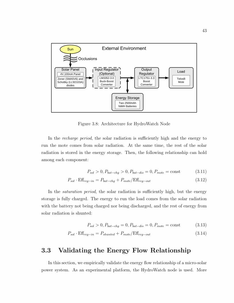
43

Two 2500mAhNiMH Batteries

LTC1751-3.3Boost

Converter

TelosBMote

4V,100mA Panel

Zener (SMA5V6) andSchottky (LLSD103A)

diodes

LM3352-3.0Buck-Boost Converter

Figure 3.8: Architecture for HydroWatch Node

In the recharge period, the solar radiation is sufficiently high and the energy to

run the mote comes from solar radiation. At the same time, the rest of the solar

radiation is stored in the energy storage. Then, the following relationship can hold

among each component:

Psol > 0, Pbat−chg > 0, Pbat−dis = 0, Pmote = const (3.11)

Psol · Effreg−in = Pbat−chg + Pmote/Effreg−out (3.12)

In the saturation period, the solar radiation is sufficiently high, but the energy

storage is fully charged. The energy to run the load comes from the solar radiation

with the battery not being charged nor being discharged, and the rest of energy from

solar radiation is shunted:

Psol > 0, Pbat−chg = 0, Pbat−dis = 0, Pmote = const (3.13)

Psol · Effreg−in = Pshunted + Pmote/Effreg−out (3.14)

3.3 Validating the Energy Flow Relationship

In this section, we empirically validate the energy flow relationship of a micro-solar

power system. As an experimental platform, the HydroWatch node is used. More

44

sol

sol bat

bat mote

mote

Figure 3.9: Energy measurement set-up with HydroWatch Node

detail of the HydroWatch node will be discussed later in Chapter 5. The summary

of the HydroWatch node is below:

• Solar Panel: 4V-100mA polycrystalline silicon panel with Zener diode (SMA5V6)

and Schottky diode (LLSD103A) for protection from high voltage and reverse

flow

• Input Regulator: two configurations, one with LM3352-3.0 buck-boost converter

as an input regulator and the other without an input regulator

• Energy Storage: Two 2500mAh NiMH batteries, series connected

• Output Regulator: LTC1751-3.3 boost converter

• Load: TelosB node running at 3mA average current

Figure 3.9 shows the experiment set-up for measuring the overall energy flow of

a HydroWatch node. A few measurement points are set up with digital multimeters

logging the voltage and the current – solar panel voltage (Vsol), solar panel current

(Isol), battery voltage (Vbat), battery charging current (Ibat), load voltage (Vmote) and

load current (Imote). The experiment has two configurations: one with an input

regulator, and the other without an input regulator.

45

3.3.1 HydroWatch Node with an Input Regulator

Figure 3.10 shows the energy flow when the HydroWatch node was configured

with an input regulator. Depending on the availability of solar radiation and the

charging status of the battery, the daily trend can be divided into different periods:

discharge before dawn (00:17:08 - 06:57:13), transition at dawn (06:57:13 - 08:47:16),

recharge (08:47:16 - 17:27:16), transition at dusk (17:27:16 - 19:27:13), and discharge

after dusk (19:27:13 - 23:57:20).

Discharge Period

During the discharge period, we can see that conditions (3.6) are met from Fig-

ure 3.10. The mote power consumption was expected to be constant, but was fluc-

tuating a bit. This was because the device was in the outdoor environment without

proper sealing: exposure to moisture increased the current consumption of the mote.

From relation (3.7), we have calculated Effout−reg of 57% for discharge before dawn

and 51% for discharge after dusk. Compared to the manufacturer-provided value 65%,

our estimations of Effout−reg have a deviation of 8% and 14%, respectively.

Transition Period

During the transition period, we can see that conditions (3.8) are met. In order to

estimate the efficiency of the input regulator Effin−reg from relation (3.7), we assumed

that the efficiency of the output regulator Effout−reg is the same as the value in the

adjacent discharge periods. The calculated input regulator efficiency is 70% for transi-

tion at dawn and 60% for transition at dusk. Compared to the manufacturer-provided

efficiency 81%, these estimations have a deviation of 11% and 21%, respectively.

Recharge Period

During the recharge period, we can see that conditions (3.11) are met. In order

to see whether the relation (3.12) holds, we take the mean values of Effin−reg and

Effout−reg from the transition and discharge periods as the input regulator efficiency

and the output regulator efficiency during the recharge period. From Figure 3.10, we

46

can evaluate the two sides of relation (3.12): the solar radiation after the input regu-

lator, Esol ·Effreg−in, is evaluated as 2604J and the energy charged to the battery, and

mote consumption, Ebat−chg + Emote/Effreg−out, is evaluated as 2459J. The difference

between the two sides of the relation is 5%, which implies that our hypothesis for

relation (3.12) holds within an error of 5%.

Saturation Period

In this experiment, we did not observe the situation for the saturation period,

where the energy flow should meet relationships (3.13).

3.3.2 HydroWatch Node without an Input Regulator

Figure 3.11 shows the energy flow when the HydroWatch node was configured

without an input regulator. As in the case with an input regulator, the daily trend

can be divided into different periods depending on the availability of solar radiation

and the charging status of the battery: discharge before dawn (00:52:20 - 07:15:32),

transition at dawn (07:15:32 - 08:05:34), recharge (08:05:34 - 18:05:34), transition at

dusk (18:05:34 - 18:25:32), and discharge after dusk (18:25:32 - 23:55:36).

Discharge Period

During the discharge period, we can see that conditions (3.6) are met from Fig-

ure 3.11. From relation (3.7), we have calculated Effout−reg of 50% for discharge before

dawn and 47% for discharge after dusk. Compared to the manufacturer-provided value

65%, our estimations of Effout−reg have a deviation of 15% and 18%, respectively.

Transition Period

The condition for the transition period (3.8) has a parameter for the efficiency of

the input regulator, while this configuration does not have an input regulator. We

can see that this condition is still met if we set the efficiency of the input regulator

as 100% (no power loss). This can be also confirmed by solving relation (3.7) for the

efficiency of the input regulator assuming that the efficiency of the output regulator

is the same as the value in the adjacent discharge periods, which gives 100% and 96%.

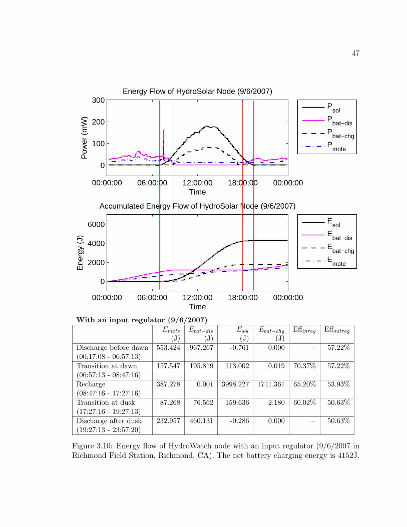
47

00:00:00 06:00:00 12:00:00 18:00:00 00:00:00

0

100

200

300

Time

Pow

er (

mW

)Energy Flow of HydroSolar Node (9/6/2007)

P

sol

Pbat−dis

Pbat−chg

Pmote

00:00:00 06:00:00 12:00:00 18:00:00 00:00:00

0

2000

4000

6000

Time

Ene

rgy

(J)

Accumulated Energy Flow of HydroSolar Node (9/6/2007)

E

sol

Ebat−dis

Ebat−chg

Emote

With an input regulator (9/6/2007)Emote Ebat−dis Esol Ebat−chg Effinreg Effoutreg

(J) (J) (J) (J)Discharge before dawn 553.424 967.267 -0.761 0.000 − 57.22%(00:17:08 - 06:57:13)Transition at dawn 157.547 195.819 113.002 0.019 70.37% 57.22%(06:57:13 - 08:47:16)Recharge 387.278 0.001 3998.227 1741.361 65.20% 53.93%(08:47:16 - 17:27:16)Transition at dusk 87.268 76.562 159.636 2.180 60.02% 50.63%(17:27:16 - 19:27:13)Discharge after dusk 232.957 460.131 -0.286 0.000 − 50.63%(19:27:13 - 23:57:20)

Figure 3.10: Energy flow of HydroWatch node with an input regulator (9/6/2007 inRichmond Field Station, Richmond, CA). The net battery charging energy is 4152J.

48

Recharge Period

During the recharge period, we can see that conditions (3.11) are met. In order

to see whether the relation (3.12) holds, we estimate the efficiencies of the input

regulator and the output regulator as 98% and 49%, which are the mean values

during transition and discharge periods. From Figure 3.11, we can evaluate the two

sides of relation (3.12): the solar radiation after the input regulator, Esol · Effreg−in,

is evaluated as 6490J and the energy charged to the battery, and mote consumption,

Ebat−chg + Emote/Effreg−out, is evaluated as 5911J. The difference between the two

sides of the relation is 9%, which implies that our hypothesis for relation (3.12) holds

within an error of 9%. Also notice that this experiment shows a weather effect in the

late afternoon, where the solar panel output power gets smaller than the envelope

and becomes irregular.

Saturation Period

In this experiment, we did not observe the situation for the saturation period,

where the energy flow should meet relationships (3.13).

3.3.3 System Efficiency

For a unit quantity of solar radiation,

Effreg−in · Effbat · Effreg−out (3.15)

is eventually used for the operation of the mote. We define (3.15) as the system

efficiency of a micro-solar power system. Table 3.4 compares the daily trends of system

efficiency for the HydroWatch node in two cases: case a with an input regulator, and

case b without an input regulator. Both cases have a similar value for the efficiency

of the output regulator (52.4% for case 1 and 48.3% for case 2), but the absence of

the input regulator makes case 2 about 50% higher in system efficiency than case 1

(21.7% for case 1 and 32.6% for case 2).

49

00:00:00 06:00:00 12:00:00 18:00:00 00:00:00

0

100

200

300

Time

Pow

er (

mW

)Energy Flow of HydroSolar Node (9/21/2007)

P

sol

Pbat−dis

Pbat−chg

Pmote

00:00:00 06:00:00 12:00:00 18:00:00 00:00:00

0

2000

4000

6000

Time

Ene

rgy

(J)

Accumulated Energy Flow of HydroSolar Node (9/21/2007)

E

sol

Ebat−dis

Ebat−chg

Emote

Without an input regulator (9/21/2007)Emote Ebat−dis Esol Ebat−chg Effinreg Effoutreg

(J) (J) (J) (J)Discharge before dawn 225.224 450.898 -0.824 0.000 − 49.95%(00:55:20 - 07:15:32)Transition at dawn 29.439 35.275 23.738 0.006 99.68% 49.95%(07:15:32 - 08:05:34)Recharge 409.010 0.014 6643.725 5068.786 97.68% 48.59%(08:05:34 - 18:05:34)Transition at dusk 11.653 14.531 10.603 0.000 95.69% 47.22%(18:05:34 - 18:25:32)Discharge after dusk 196.609 416.336 0.423 0.000 − 47.22%(18:25:32 - 23:55:36)

Figure 3.11: Energy flow of HydroWatch node without an input regulator (9/21/2007in Richmond Field Station, Richmond, CA). The net battery charging energy is 44J.

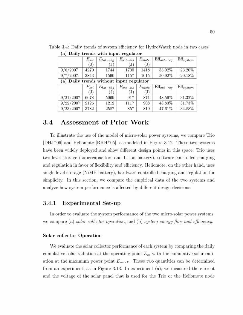
50

Table 3.4: Daily trends of system efficiency for HydroWatch node in two cases

(a) Daily trends with input regulatorEsol Ebat−chg Ebat−dis Emote Effout−reg Effsystem(J) (J) (J) (J)

9/6/2007 4270 1744 1700 1418 53.92% 23.20%9/7/2007 3843 1590 1157 1015 50.92% 20.18%(a) Daily trends without input regulator

Esol Ebat−chg Ebat−dis Emote Effout−reg Effsystem(J) (J) (J) (J)

9/21/2007 6678 5069 917 871 48.59% 31.32%9/22/2007 2126 1212 1117 908 48.83% 31.73%9/23/2007 3782 2587 857 819 47.61% 34.88%

3.4 Assessment of Prior Work

To illustrate the use of the model of micro-solar power systems, we compare Trio

[DHJ+06] and Heliomote [RKH+05], as modeled in Figure 3.12. These two systems

have been widely deployed and show different design points in this space. Trio uses

two-level storage (supercapacitors and Li-ion battery), software-controlled charging

and regulation in favor of flexibility and efficiency. Heliomote, on the other hand, uses

single-level storage (NiMH battery), hardware-controlled charging and regulation for

simplicity. In this section, we compare the empirical data of the two systems and

analyze how system performance is affected by different design decisions.

3.4.1 Experimental Set-up

In order to evaluate the system performance of the two micro-solar power systems,

we compare (a) solar-collector operation, and (b) system energy flow and efficiency.

Solar-collector Operation

We evaluate the solar collector performance of each system by comparing the daily

cumulative solar radiation at the operating point Eop with the cumulative solar radi-

ation at the maximum power point EmaxP . These two quantities can be determined

from an experiment, as in Figure 3.13. In experiment (a), we measured the current

and the voltage of the solar panel that is used for the Trio or the Heliomote node

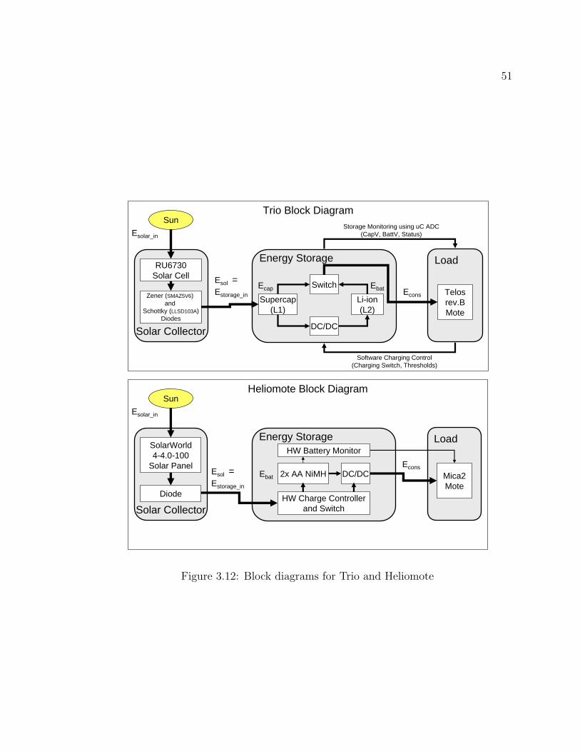
51

Trio Block Diagram

Load

Telosrev.BMote

RU6730Solar Cell

Zener (SMAZ5V6) and

Schottky (LLSD103A)Diodes

Supercap(L1)

DC/DC

Software Charging Control(Charging Switch, Thresholds)

Storage Monitoring using uC ADC(CapV, BattV, Status)

SunEsolar_in

Estorage_in EconsLi-ion(L2)

Solar Collector

Switch

Energy Storage

Esol = Ecap Ebat

Heliomote Block Diagram

Load

Mica2Mote

SolarWorld4-4.0-100

Solar Panel

Diode

2x AA NiMH

HW Charge Controllerand Switch

SunEsolar_in

Estorage_in

Econs

Solar Collector

Energy Storage

DC/DC

HW Battery Monitor

Esol = Ebat

Figure 3.12: Block diagrams for Trio and Heliomote

52

A

V Solar-PoweredSensor Node-

+

(a) Operating point (Iop, Vop) is measured (b) I-V curve is measured

Figure 3.13: Experimental set-up for measuring solar panel output power.

(Iop, Vop). This is characteristic of the solar panel at its operating point. In experiment

(b), we measured a sequence of (I,V) values for a separate solar panel by adjusting the

load impedance. Based on this I-V curve, the maximum power point (ImaxP , VmaxP )

can be found where the solar panel output power P = I · V is maximized.

Energy Flow and Energy Efficiency

We evaluate the performance of the overall system by comparing the energy effi-

ciency of a micro-solar power system. Depending on system status, the system energy

efficiency can be defined as follows:

• Daily System-wide efficiency:

Effsys = (∆Ebat + ∆Ecap + ∆Econs)/∆Esol

This metric represents how much of the daily solar radiation energy is used for

battery charging, supercapacitor charging and mote consumption.

• Battery discharging efficiency:

Effbat−dis = ∆Econs/∆Ebat−dis

In darkness, the system runs on the energy that is discharged from the battery or

the supercapacitor. This metric represents how much of the energy discharged

from the battery is used for the mote operation during a battery discharge

period.

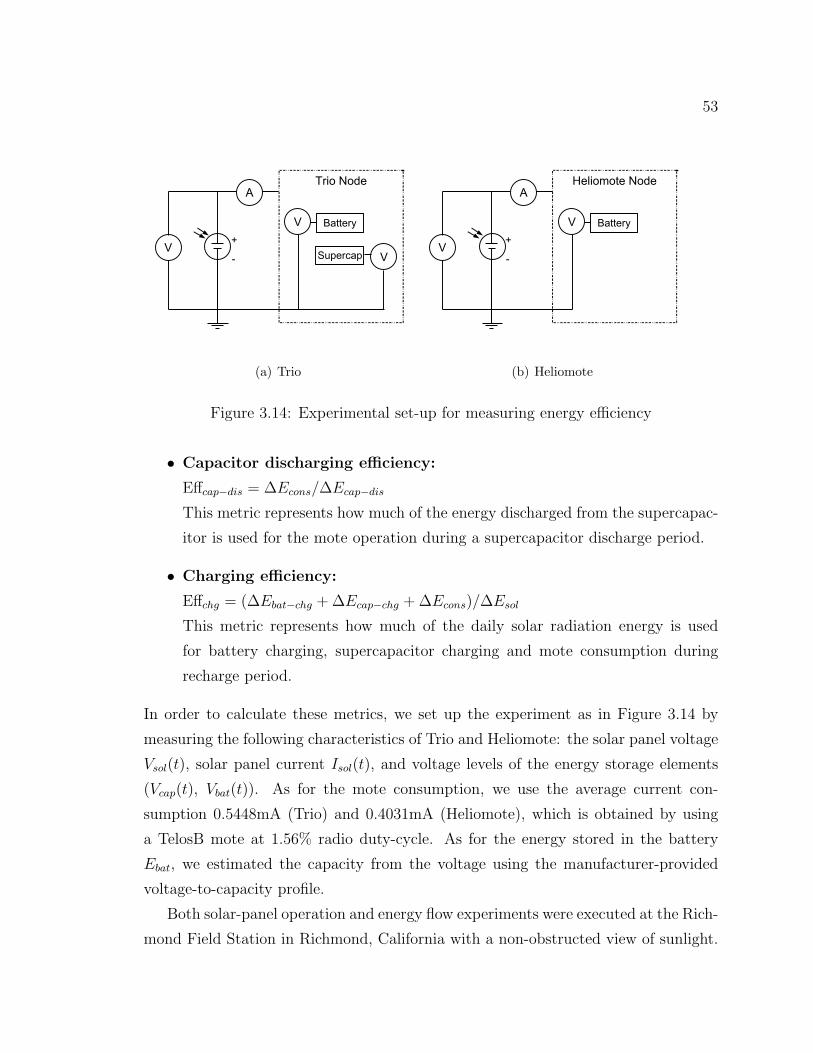
53

A

V

Trio Node

VVSupercap

Battery

-

+

(a) Trio

A

V

Heliomote Node

V

Battery

-

+

(b) Heliomote

Figure 3.14: Experimental set-up for measuring energy efficiency

• Capacitor discharging efficiency:

Effcap−dis = ∆Econs/∆Ecap−dis

This metric represents how much of the energy discharged from the supercapac-

itor is used for the mote operation during a supercapacitor discharge period.

• Charging efficiency:

Effchg = (∆Ebat−chg + ∆Ecap−chg + ∆Econs)/∆Esol

This metric represents how much of the daily solar radiation energy is used

for battery charging, supercapacitor charging and mote consumption during

recharge period.

In order to calculate these metrics, we set up the experiment as in Figure 3.14 by

measuring the following characteristics of Trio and Heliomote: the solar panel voltage

Vsol(t), solar panel current Isol(t), and voltage levels of the energy storage elements

(Vcap(t), Vbat(t)). As for the mote consumption, we use the average current con-

sumption 0.5448mA (Trio) and 0.4031mA (Heliomote), which is obtained by using

a TelosB mote at 1.56% radio duty-cycle. As for the energy stored in the battery

Ebat, we estimated the capacity from the voltage using the manufacturer-provided

voltage-to-capacity profile.

Both solar-panel operation and energy flow experiments were executed at the Rich-

mond Field Station in Richmond, California with a non-obstructed view of sunlight.

54

Fluke-189 data logging multimeters were used to record measurements. In comparing

the two systems, we focus on high radiation hours (9AM to 5PM), because the solar

panel output current is too small for practical use outside this window of time.

3.4.2 Solar-collector Operation

A series of solar panel I-V curves for Trio and Heliomote are shown in Figure 3.15,

and each I-V curve is marked with the corresponding operating point and the max-

imum power point. Figure 3.16(a) compares the solar panel output power at the

operating point Pop and the maximum power point PmaxP , and it shows that the

solar collector of Trio is better matched to the maximum power point than that of

Heliomote. Figure 3.16(b) gives a more quantitative sense of the possible energy

savings from operating point matching. The deviation of the daily cumulative en-

ergy at operating point Eop from the daily cumulative energy at MPP EmaxP is 4.8%

(Eop = 3203J and EmaxP = 3055J) for Trio whereas it is 22.0% (Eop = 1712J and

EmaxP = 2195J) for Heliomote.

This gap happens because the way the solar panel and the energy energy are

matched is different for the two systems (Figure 3.17). For Trio, solar panel output

is buffered in the supercapacitor before charging the battery. The supercapacitor

operates between 3.2V and 4.0V. This range is set by thresholds Vcap−lb and Vcap−ub in

the software-based charging controller (Figure 3.18). The overload protection voltage

Voverload is set to 5.1V by the reverse-biased Zener diode. Thus, the solar panel output

can be transferred to the supercapacitor and the battery without being cut by the

overload protection circuit. Heliomote, on the other hand, charges the solar-panel

output to the battery without buffering, and the solar-panel operating voltage Vop is

clipped to the overload protection voltage Voverload (= 2.8V). While this protects the

battery from overload, more of the energy from the solar panel is wasted, causing the

larger deviation from PmaxP .

Figure 3.19 shows the relationship between the solar panel output power, Pop and

the operating voltage, Vop for the two systems. Pop is close to zero for a large range of

voltage levels, but rises sharply once the voltage is past a certain threshold (3.7V for

Trio and 2.8V for Heliomote). This implies that the useful (most power produced)

range of the solar panel in a particular system is very narrow. Therefore, power

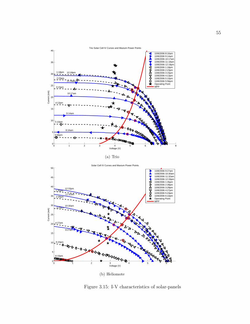
55

0 1 2 3 4 5 6 7 80

5

10

15

20

25

30

35

40

Voltage (V)

Cur

rent

(m

A)

Trio Solar Cell IV Curves and Maxium Power Points

10/8/2006 8:16am10/8/2006 9:14am10/8/2006 10:17am10/8/2006 11:18am10/8/2006 12:18pm10/8/2006 1:18pm10/8/2006 2:23pm10/8/2006 3:15pm10/8/2006 4:13pm10/8/2006 5:10pm10/8/2006 5:56pmOperating PointMPP

5:56pm

5:10pm

4:13pm

3:15pm

2:23pm

1:18pm

8:16am

9:14am

10:17am

11:18am

12:18pm

(a) Trio

0 1 2 3 4 5 60

5

10

15

20

25

30

35

40

45

50

Voltage (V)

Cur

rent

(m

A)

Solar Cell IV Curves and Maxium Power Points

10/8/2006 9:27am10/8/2006 10:30am10/8/2006 11:32am10/8/2006 12:33pm10/8/2006 1:35pm10/8/2006 2:39pm10/8/2006 3:29pm10/8/2006 4:27pm10/8/2006 5:23pm10/8/2006 6:10pmOperating PointMPP

9:27am

10:30am

11:32am

12:33pm1:35pm

2:39pm

3:29pm

4:27pm

5:23pm

6:10pm

(b) Heliomote

Figure 3.15: I-V characteristics of solar-panels

56

06:00 09:00 12:00 15:00 18:00 21:000

50

100

150

Time

Pow

er (

mW

)

Comparison of solar panel output power: operating point vs MPP(Trio on 10/8/2006)

Operating pointMPP

06:00 09:00 12:00 15:00 18:00 21:000

500

1000

1500

2000

2500

3000

3500

Time

Ene

rgy

(J)

Comparison of daily cumulative solar radiation: operating point vs MPP(Trio on 10/8/2006)

Operating pointMPP

06:00 09:00 12:00 15:00 18:00 21:000

50

100

150

Time

Pow

er (

mW

)

Comparison of solar panel output power: operating point vs MPP(Heliomote on 10/8/2006)

Operating pointMPP

06:00 09:00 12:00 15:00 18:00 21:000

500

1000

1500

2000

2500

Time

Ene

rgy

(J)

Comparison of daily cumulative solar radiation: operating point vs MPP(Heliomote on 10/8/2006)

Operating pointMPP

(a) Solar panel output power06:00 09:00 12:00 15:00 18:00 21:000

50

100

150

Time

Pow

er (

mW

)

Comparison of solar panel output power: operating point vs MPP(Trio on 10/8/2006)

Operating pointMPP

06:00 09:00 12:00 15:00 18:00 21:000

500

1000

1500

2000

2500

3000

3500

Time

Ene

rgy

(J)

Comparison of daily cumulative solar radiation: operating point vs MPP(Trio on 10/8/2006)

Operating pointMPP

06:00 09:00 12:00 15:00 18:00 21:000

50

100

150

Time

Pow

er (

mW

)

Comparison of solar panel output power: operating point vs MPP(Heliomote on 10/8/2006)

Operating pointMPP

06:00 09:00 12:00 15:00 18:00 21:000

500

1000

1500

2000

2500

Time

Ene

rgy

(J)

Comparison of daily cumulative solar radiation: operating point vs MPP(Heliomote on 10/8/2006)

Operating pointMPP

(b) Cumulative solar radiation

Figure 3.16: Comparison of solar panel output power and cumulative solar radiation

57

0 1 2 3 4 5 6 7 80

10

20

30

40


So

lar

Pan

el C

urr

ent

(mA

)Effects of Regulator on Solar−Panel (Trio)

Voverload

Vop

Vcap

0 1 2 3 4 5 60

10

20

30

40

50Effects of Regulator on Solar−Panel (Heliomote)


So

lar

Pan

el C

urr

ent

(mA

)

Voverload

Vop

Figure 3.17: Comparison of regulator designs

Table 3.5: Component energy level and system energy efficiency for Trio andHeliomote

Trio Date 10/9/06 10/11/06 10/12/06∆Esol 3031.3J 2885.5J 2870.8J∆Ecap -0.05J -0.04J 0.16J∆Ebat 791.2J 342.1J 348.8J∆Econs 221.0J 220.3J 221.0JEffsys 33.4% 19.5% 19.8%

Heliomote Date 10/14/06 10/16/06 10/18/06∆Esol 1237.6J 1449.9J 1641.4J∆Ebat 27.0J 107.3J 10.1J∆Econs 10.0J 104.5J 103.0JEffsys 10.5% 14.6% 6.9%

tracking circuits or algorithms are only meaningful within this small range.

3.4.3 Energy Flow and Energy Efficiency

The trend of daily energy flow and system energy efficiency for the two micro-

solar power systems is summarized in Table 3.5. From this result, we can observe the

following: First, the net battery energy level has increased, which means that Trio

and Heliomote have excess energy to store even after mote consumption and energy

losses. Second, the supercapacitor of the Trio node stays at about the same energy

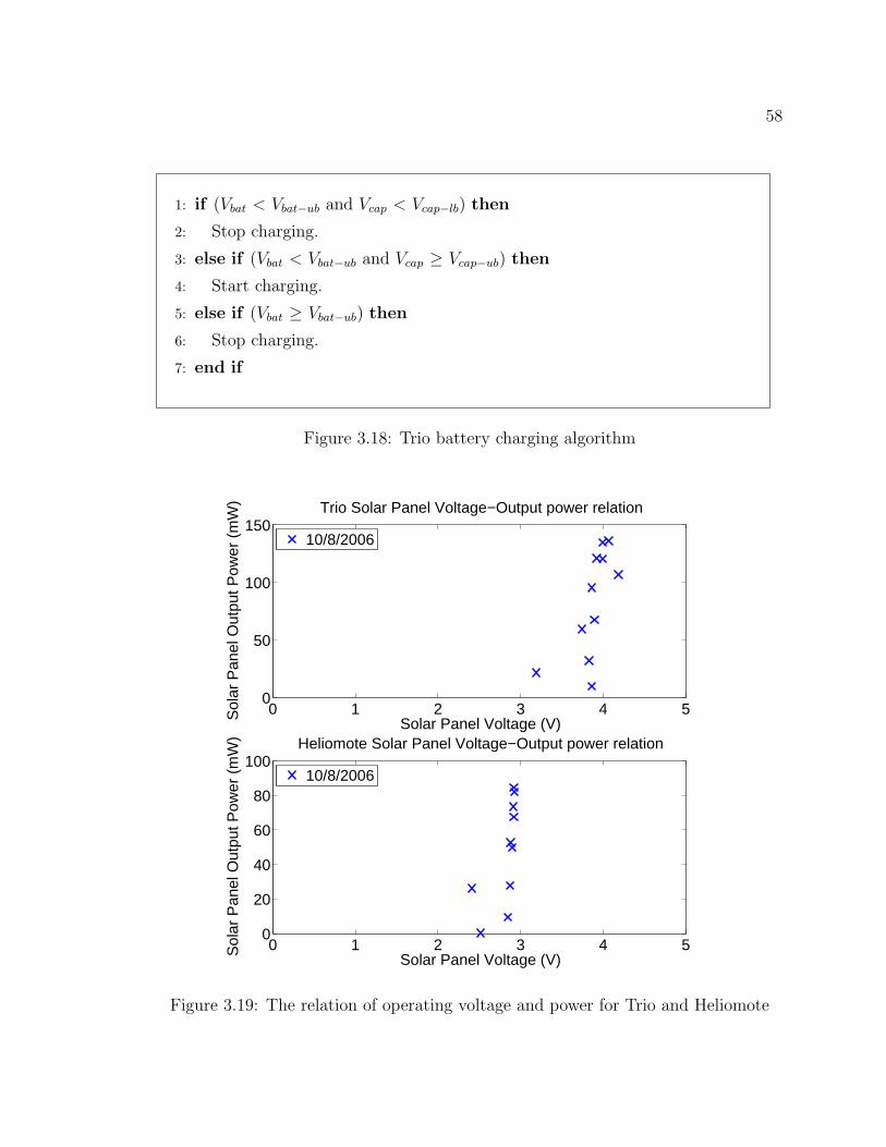
58

1: if (Vbat < Vbat−ub and Vcap < Vcap−lb) then

2: Stop charging.

3: else if (Vbat < Vbat−ub and Vcap ≥ Vcap−ub) then

4: Start charging.

5: else if (Vbat ≥ Vbat−ub) then

6: Stop charging.

7: end if

Figure 3.18: Trio battery charging algorithm

0 1 2 3 4 50

50

100

150

Solar Panel Voltage (V)Sol

ar P

anel

Out

put P

ower

(m

W) Trio Solar Panel Voltage−Output power relation

10/8/2006

0 1 2 3 4 50

20

40

60

80

100

Solar Panel Voltage (V)Sol

ar P

anel

Out

put P

ower

(m

W) Heliomote Solar Panel Voltage−Output power relation

10/8/2006

Figure 3.19: The relation of operating voltage and power for Trio and Heliomote

59

Table 3.6: Energy efficiency of charging and discharging for Trio and Heliomote

Trio Date 10/9/06 10/11/06 10/12/06Effchg 46.9% 31.2% 28.5%Effbat−dis 24.5% 32.7% 34.9%Effcap−dis 57.2% 54.3% 68.6%

Heliomote Date 10/14/06 10/16/06 10/18/06Effchg 52.0% 45.5% 54.2%Effbat−dis 35.6% 32.2% 32.7%

level each day, with a net increase close to zero. This implies that the supercapacitor

buffers the solar energy, and transfers the excess energy to the battery. Further, the

net battery energy increase ∆Ebat is positively correlated with the daily solar energy

budget ∆Esol. Finally, our experimental data shows that for the Trio node, 19.5% to

33.4% of the available solar energy is charged to storage or consumed by the mote,

while the Heliomote node has an energy efficiency between 6.9% to 14.6%. As for

the weather condition for the measurement on each day, we chose sunny days in mid-

October so that the weather condition would be similar in all the measurements. One

difference between the measurements of each day is the energy level of the storage

elements, because we used the same experiment set-up over multiple days without

depleting the energy storage. This explains the difference in the energy level of the

storage elements (∆Ebat).

In order to calculate the charging and discharging efficiencies, we can divide the

operating range of Trio and Heliomote into multiple phases as shown in Figure 3.20:

battery discharge period (D1), capacitor discharge period (D2), recharge period (C),

and saturation period (S). The balance of the energy level of each component for these

phases are shown in Figure 3.21.

The charging and discharging efficiency results are summarized in Table 3.6. The

Trio node has both a battery discharge period and a capacitor discharge period be-

cause it has two-level storage of a supercapacitor and Li-ion battery. Trio also has

a recharge period, but not a saturation period. We observed a battery discharging

efficiency of 24.5% to 34.9%, capacitor discharging efficiency of 54.3% to 68.6%, and

charging efficiency of 28.5% to 46.9%. The Heliomote node has a battery discharge

period and a recharge period. It has a saturation period because the charging pro-

tection circuit is activated during its operation. We observed a battery discharging

60

00:00 06:00 12:00 18:00 00:00−500

0

500

1000

1500

2000

2500

3000

3500

Time

Ene

rgy

(J)

Daily energy trend for Trio node on 10/12/2006

E

sol

Ebat

Ecap

Econs

D1 C D2 D1

00:00 06:00 12:00 18:00 00:00−500

0

500

1000

1500

2000

Time

Ene

rgy

(J)

Daily energy trend for Heliomote node on 10/14/2006

E

sol

Ebat

Econs

D1 C S D1

Figure 3.20: Daily energy flow of Trio and Heliomote

61

D1 C D2 D10

500

1000

1500

2000

2500

3000

3500

4000

Energy supplied from solar panel or storage for Trio on 10/12/2006

Ene

rgy

(J)

Phase

solarbat dischargecap discharge

D1 C D2 D10

500

1000

1500

2000

2500

3000

3500

4000

Energy consumed or stored for Trio on 10/12/2006

Ene

rgy

(J)

Phase

motebat chargecap charge

D1 C S D10

500

1000

1500

Energy supplied from solar panel or storage for Heliomote on 10/14/2006

Ene

rgy

(J)

Phase

solarbat discharge

D1 C S D10

500

1000

1500

Energy consumed or stored for Heliomote on 10/14/2006

Ene

rgy

(J)

Phase

motebat charge

Figure 3.21: Energy flow of Trio and Heliomote at different phases

62

efficiency of 32.2% to 35.6% and charging efficiency of 45.5% to 54.2%.

We can see that the charging and discharging efficiency of Heliomote is as good as

that of Trio, but its system efficiency (6.9% to 14.6%) is much smaller than that of

Trio (19.5% to 33.4%). This is because much of the solar energy is wasted during the

saturation period; at a lower battery capacity, the system efficiency would be higher.

If we assume that Heliomote does not go through the saturation period and utilizes

the solar energy during saturation period at the same rate as in recharge period, then

the system efficiency would be 31.9% to 41.9%.

3.5 Summary of Micro-solar Power System Archi-

tecture

In this chapter, we have introduced an architecture for micro-solar power systems

by exploring the characteristics of each constituent component. The behavior of each

component and its interactions with other components can be summarized in the

following way:


The radiation condition at a certain time and location is described by radiation

rate RR, which is a real number between 0 and 1. The radiation rate is determined

by either an astronomical model or an astronomical model with local enhancements:

RR ∈ [0,1] (3.16)

Solar Collector

The operating point of a solar panel is described by the I-V curve of the panel,

which is determined by a sequence of (I,V) pairs taken from empirical measurement.

The current of the solar panel under this radiation rate, Irad, is given by the product

of the radiation rate RR and the solar panel current in the I-V curve Ipanel.

Ipanel = IVCurve(Vpanel) (3.17)

Irad = RR · Ipanel (3.18)

63

Energy Storage

The energy storage is described by its voltage level, energy level and charge-

discharge efficiency. The voltage-to-energy relationship, which is usually given by

the manufacturer, describes the relationship between the voltage level and the energy

level of the energy storage. The charge-discharge efficiency, which depends on the

technology of the energy storage, describes how much energy can be discharged when

a given energy is charged.

Vstor = E-to-V(Estor)⇔ Estor = V-to-E(Vstor) (3.19)

Edischarged = Effstor · Echarged (3.20)

Input Regulator

The operation of an input regulator is described by its power efficiency and a

transfer function. The power delivered out of an input regulator is proportional

to the power from the solar panel and the power efficiency of the input regulator,

which depends on the solar panel voltage, the solar panel current and the energy

storage voltage. The input regulator sets the operating point of the solar panel,

interconnecting with the energy storage. Depending on the type of input regulator

being used (e.g. no-input regulator or constant-input-voltage regulator), the voltage

of the solar panel can follow the voltage of the energy storage, or can be set to a

constant.

Pin−reg = Effin−reg · Ppanel (3.21)

Vpanel = Vstor + Vth or const (3.22)

Output Regulator

The operation of an output regulator is described by power efficiency and the

output voltage. The power efficiency of an output regulator is dependent on the en-

ergy storage voltage and the load current. The output voltage of an output regulator

is relatively constant over its operating range. The power consumption of an out-

put regulator is proportional to the power consumption of the load and inversely

64

proportional to the power efficiency.

Vout−reg = const (3.23)

Pout−reg =1

Effout−reg· Pload (3.24)

Load

The operation of the load is described by its average current and operating voltage.

The average current is determined by the application, and the operating voltage is

determined by the output regulator.

Iload : given by application (3.25)

Vload = Vout−reg (3.26)

Overall System Behavior

Once the behavior of the components of a micro-solar power system and their

interconnections are defined, the system behavior can be described as follows:

• Surplus power from the solar radiation after being used for load:

Pnet = Pin−reg − Pout−reg (3.27)

• If the surplus is positive (Pnet > 0),

System is in recharge state with energy of Pnet ·∆t being charged.

• If the surplus is non-positive (Pnet ≤ 0),

System is in discharge state with energy of (-Pnet) ·∆t being discharged.

• Change of the energy level and the voltage of the energy storage:

Estor = Estor + Pnet ·∆t (3.28)

Vstor = E-to-V(Estor) (3.29)

In the next chapter, we construct a micro-solar power system simulator based on

this architecture.

65

Chapter 4

Design of Micro-Solar Power

System Simulator

One of the difficulties of building a network of micro-solar power systems is that

the whole process of design, development and deployment takes a long time. Suppose

a micro-solar power system is deployed in an outdoor environment. It may have an

energy surplus for a few days or even several months, but, depending on the weather

or other conditions that affect solar radiation, it can either keep accumulating solar

energy or may lose stored battery energy, becoming unable to provide energy for

perpetual operation. This is because the operation of a micro-solar power system

depends greatly on the characteristics of the environment and each component. In

order to have a reasonable estimation of system behavior we may take extensive mea-

surements over time, but this can make the whole process of design, development

and deployment even longer. What we need is a design and simulation tool that

allows us to estimate the behavior of a micro-solar power system with sufficient accu-

racy over the long term without taking the time and effort of an actual development

and deployment. In this chapter, we present a Matlab-based micro-solar power sys-

tem simulator and describe its key ideas. The simulator takes a configuration of a

micro-solar power system along with user-defined data and quickly generates behavior

estimates for either a short period or a long period of time. The rest of this chapter

is organized as follows: first, Section 4.1 states an overall architecture and principles

for the micro-solar power system simulator; then, Sections 4.2 through 4.7 describe

66

key implementation ideas that translate each component of a micro-solar power sys-

tem into the framework of the simulator; finally, Section 4.8 validates the simulation

model with benchtop experiments.

4.1 Overall Architecture and Principles

4.1.1 Modularity

The simulator is composed of the following modules: external environment mod-

ule, solar panel module, input regulator module, energy storage module, output regu-

lator module and load module. Each module of the simulator describes the behavior

of a corresponding component of a micro-solar power system (Figure 4.1). Each simu-

lator module can be exchanged with another module in the same class. For example,

a definition of 3.6V-50mA flexible solar panel can be used instead of a definition of

4V-100mA solar panel without changing other parts of the simulator. In the simu-

lator, the internal operation of each component is hidden, so in order to access the

characteristic of each component, a user should use a function that describes the

component.

4.1.2 Time-Event Based Simulator

Our simulator computes the state of each component of a micro-solar power system

when the initial condition (e.g. initial battery capacity) and the time-event vector are

given. (Figure 4.2(a)). The time-event vector is a tuple of discrete times during the

day at which the state of the micro-solar power system will be evaluated. For example,

the time-event vector can be given as [t0, t1, t2, t3, · · · , tn] = [0, 0.25, 0.5, 0.75, · · · , 24]

for simulating system status on a particular day at 15 minute interval starting from

midnight. Overall, the estimation accuracy increases as the interval between the

evaluation times gets smaller, but, at the same time, the computation time increases

in proportion to the inverse of the interval. Once the state of the micro-solar power

system is computed for one day, the long-term trend can be computed iteratively as

is illustrated in Figure 4.2(b); the state of the system is evaluated with the result of

one day being the initial condition of the next day.

67

Supercap with Vmax ,capacity C and

leakage current Ic

Energy Storage


…


Output Regulator




Input Regulator



Activity Model

Load


…Application CodeBased Model

3.6V-50mA FlexibleAmorphous Silicon Panel

Solar Panel

4V-100mA PolycrystallineSilicon Panel

…


AstronomicalModel

…StatisticalModel

ObstructedAstronomical

Model

Constant RadiationModel

Figure 4.1: Modular design of micro-solar power system simulator

68

InitialCondition

T0

[t0, t1]T1

[t1, t2]Tn-1

[tn-1, tn]…

Estimator

State(T0) State(T1) State(Tn-1)…

(a) Estimation of daily trend

InitialCondition

T0

[t0, t1]T1

[t1, t2]Tn-1

[tn-1, tn]…

Estimator (Step 2)


T0

[t0, t1]T1

[t1, t2]Tn-1

[tn-1, tn]…

Estimator (Step 1)


T0

[t0, t1]T1

[t1, t2]Tn-1

[tn-1, tn]

Estimator (Step N)


…

… …

Day 1

Day 2

Day N

(b) Estimation of long-term trend

Figure 4.2: Time-event based simulator

69

4.1.3 Defining a Component Using User-provided Data

A component of a micro-solar power system has a common generic behavior, but

its detailed behavior may vary depending on what instance of a component is used.

Our simulator provides two different ways to customize the behavior of a component:

curve-fitting and piecewise linear interpolation.

The curve-fitting method is used when the behavior of a component can be

described by a formula. A formula generally consists of a collection of variables,

constants and operators. When measurements of the component are available, the

curve-fitting algorithm determines the unknown constants that minimize the errors

between the measured output and the estimated output. The solar-panel IV charac-

teristic is one example where the curve fitting method is used. Figure 4.3 shows

that the I-V characteristic of a solar panel can be described as a generic curve

I = Isc − A · (exp(B · V ) − 1). This formula describes the relationship between

the solar panel voltage V and the solar panel current I. Each instance of this solar

panel model describes a different type of solar panel simply by altering the values for

the parameters Isc, A, and B.

Piecewise linear interpolation is used when the behavior of a component cannot be

represented by a single formula. In order to represent the behavior of a component

with a known formula, piecewise linear interpolation partitions the input domain.

Suppose the input signal of a component operates in domain D. Then the domain

can be partitioned into D1, D2, D3, · · · , Dn so that the behavior of the component can

be described with linear functions f1, f2, f3, · · · , fn in each partition of the domain

(Figure 4.4). Here are a few examples that can be described by piecewise linear

interpolation:

• The output voltage of a regulator over its load current

• The efficiency of a regulator over its load current

• The voltage level of a battery over its capacity

In order to define the domain partitions and the piecewise linear functions, the piece-

wise linear interpolation method takes a sequence of value pairs: (x1, y1), (x2, y2),

(x3, y3), · · · (xn, yn), (xn+1, yn+1). Then, the domain partitions Di and the piecewise

70

Generic Formula

Curve Fitting

Measurement Data

Instantiated Formula

0 0.5 1 1.5 2 2.5 3 3.5 4 4.50

50

100

150


Sol

ar P

anel

Cur

rent

(mA

)

Solar Panel IV Characteristic

IV Curve

0 0.5 1 1.5 2 2.5 3 3.5 4 4.50

50

100

150


Sol

ar P

anel

Cur

rent

(mA

)


00


Sola

r Pan

el C

urre

nt (m

A) Solar-Panel I-V Curve

I = Isc - A ⋅ (exp(B ⋅ V) -1)

IV curve for a 4V-100mA polycrystalline silicon solar-panel with A = 0.2526, B = 1.4255 and Isc = 111.160

IV curve for a generic solar-panel Measurement of points of I-V pairs for a 4V-100mA polycrystalline silicon solar-panel

Figure 4.3: Defining a component using user-provided data: curve-fitting method

2 2.5 3 3.5 4 4.50

0.1

0.2

0.3

0.4

0.5

0.6

0.7

0.8

0.9

1

Input Voltage (V)

Effi

cien

cy

Illustration of Piecewise Interpolation Method

D4

D2 D

3D

1

f1

f2

f3

f4

Figure 4.4: Defining a component using user-provided data: piecewise linear interpo-lation method

71

linear function fi are determined as follows:

Di = [xi, xi+1] (4.1)

fi =yi+1 − yixi+1 − xi

(D − xi) + yi (4.2)

The algorithm in Figure 4.19 estimates the voltage level of a NiMH battery for a

given capacity using piecewise linear interpolation by fitting chords to the curve.

4.1.4 Wiring Components

In our micro-solar power simulator, we use function calls and a sequence of state-

ments to wire components to each other. We modularize this so that the wiring can be

done by plugging components into each other, with all the constraints hidden inside

the components.

4.2 Modeling Solar Radiation

Our simulator provides a few of ways to model solar radiation: an astronomical

model, a statistical model and an astronomical model with obstruction vector.

4.2.1 Astronomical Model

The astronomical model, which is based on the algorithm by Dave et al. [DHM75]

(Figure 3.2 in Chapter 3.1.1), estimates the solar radiation rate by calculating the

angle Θ (0◦ ≤ Θ ≤ 180◦) between the sunlight and the normal to the solar panel.

Depending on whether the sunlight is above or below the horizon, the solar radiation

rate is given as cos Θ (when 0◦ ≤ Θ ≤ 90◦) or 0 (when 90◦ ≤ Θ ≤ 180◦). Thus, the

solar radiation rate can be represented as max(cos Θ, 0).

The solar radiation rate max(cos Θ, 0) is a function of several parameters that

affect the time variation (t, n) and installation variation (L, θp, φp, τ):

• t : Hour of the day (0 ≤ t ≤ 24)

• n : Day of the year (1 ≤ n ≤ 365)

72

• L : Latitude (−90◦ ≤ L ≤ 90◦)

• θp : Tilted angle of solar panel (0◦ ≤ θp ≤ 180◦)

• φp : Azimuth angle, panel orientation from north (0◦ ≤ φp ≤ 360◦). For

example, 90 for the east, 180 for the south, and 270 for the west.

• τ : Atmospheric attenuation effect factor (0 ≤ τ ≤ 1)

Then, cos Θ can be given as follows:

cos Θ = cos θp · cos θs + sin θp · sin θs · cos(φp − φs) (4.3)

The intermediate terms θs, φs, h, x, δ are also given as follows:

• θs : Angle between solar radiation and local vertical (0◦ ≤ θs ≤ 180)

cos θs = sin δ · sinL+ cos δ · cosL · cosh

• φs : Angle between solar radiation and local north (−180◦ ≤ φs ≤ 180◦)

sinφs = − cos δ · sinh/ sin θs

• h : Hour angle (−180◦ ≤ h ≤ 180◦)

h = 15(t− 12)

• x : Day of the year in radian (0 ≤ x ≤ 2π)

x = 2πn/365

• δ : Declination of sun (−90◦ ≤ δ ≤ 90◦)

δ = 0.302− 22.93 cosx− 0.229 cos 2x− 0.243 cos 3x

+ 3.851 sinx+ 0.002 sin 2x− 0.055 sin 3x

The algorithm for calculating the solar radiation rate is given in Figure 4.5 and

4.6.

Figures 4.7, 4.8 and 4.9 show the estimation of the daily solar radiation for different

sets of parameters: time of the year n (Figure 4.7), latitude L (Figure 4.8), and

inclination θp and panel orientation φp (Figure 4.9).

73

function radiation_rate = calc_daily_solar_radiation(t, n, L, ...theta_p, phi_p, tau, ob_th)

% variables that can be calculated from user parametersN = max(size(t)); % size of th = 15 * (t - 12); % hour angle in degree, -180 to 180h_rad = 2 * pi * h / 360; % hour angle in radiancos_h = cos(h_rad); % cos(h_rad)theta_p_rad = 2 * pi * theta_p / 360; % tilted angle in radianL_rad = 2 * pi * L / 360; % latitude in radiantan_L = tan(L_rad); % tan(L_rad)x = 2 * pi * n / 365; % day of the year in radianphi_p_rad = 2 * pi * phi_p / 360; % azimuth angle in radian

% declination of sun in degreedelta = 0.302-22.93*cos(x)-0.229*cos(2*x)-0.243*cos(3*x) + ...

3.851 * sin(x) + 0.002 * sin(2*x) - 0.055 * sin(3*x);delta_rad = 2 * pi * delta / 360; % declination of sun in radiantan_delta = tan(delta_rad); % tan(delta_rad)

% angle b/w solar radiation and local verticalcos_theta_s = sin(delta_rad) * sin(L_rad) + ...

cos(delta_rad) * cos(L_rad) .* cos(h_rad);theta_s_rad = acos (cos_theta_s);sin_theta_s = sin(theta_s_rad);

% angle b/w solar radiation and local northsin_phi_s = -1*cos(delta_rad) .* sin(h_rad) ./ sin(theta_s_rad);phi_s_rad = asin (sin_phi_s);phi_sn_rad = zeros(N,1);for i=1:N,

if (cos_h(i,1) >= tan_delta / tan_L)phi_sn_rad(i,1) = pi + phi_s_rad(i,1);

elseif (h(i,1) < 0)phi_sn_rad(i,1) = 2 * pi - phi_s_rad(i,1);

elsephi_sn_rad(i,1) = 0 - phi_s_rad(i,1);

end;endcos_phi_s = cos (phi_s_rad);

Figure 4.5: Matlab algorithm for estimating solar radiation using an astronomicalmodel

74

% effective solar radiation coefficientcos_Z = cos(theta_p_rad) .* cos(theta_s_rad) + ...sin(theta_p_rad).*sin(theta_s_rad).*cos(phi_p_rad - phi_sn_rad);

Z_rad = acos(cos_Z);

% attenuation factorattenuation_factor = exp(-1 * tau ./ cos_theta_s);

horizon = zeros(N,1);obstruction_factor = zeros(N,1);

for i=1:N,if (theta_s_rad(i,1) <= (pi / 2))

horizon(i,1) = 1;elseif (theta_s_rad(i,1) > (pi / 2))

horizon(i,1) = 0;end;

end

% panel output rateradiation_rate = horizon .* max(cos_Z, 0) .* attenuation_factor;

Figure 4.6: Matlab algorithm for estimating solar radiation using an astronomicalmodel (continued)

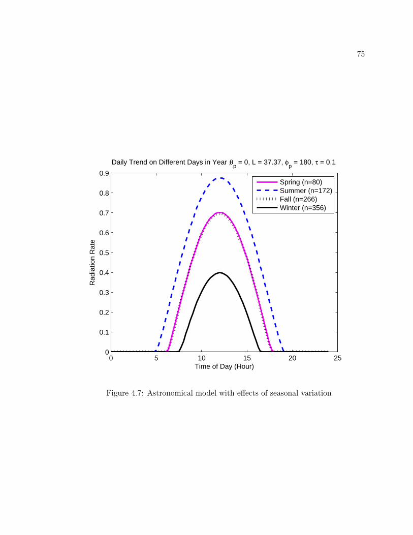
75

0 5 10 15 20 250

0.1

0.2

0.3

0.4

0.5

0.6

0.7

0.8

0.9

Time of Day (Hour)

Rad

iatio

n R

ate

Daily Trend on Different Days in Year , θp = 0, L = 37.37, φ

p = 180, τ = 0.1

Spring (n=80)Summer (n=172)Fall (n=266)Winter (n=356)

Figure 4.7: Astronomical model with effects of seasonal variation

76

0 5 10 15 20 250

0.1

0.2

0.3

0.4

0.5

0.6

0.7

0.8

0.9

1

Time of Day (Hour)

Rad

iatio

n R

ate

Daily Trend on Different Latitude , θp = 0, n = 80, φ

p = 180, τ = 0.1

L = 0L = 30L = 60L = 90

(a) Spring and fall

0 5 10 15 20 250

0.1

0.2

0.3

0.4

0.5

0.6

0.7

0.8

0.9

Time of Day (Hour)

Rad

iatio

n R

ate


p = 180, τ = 0.1

L = 0L = 30L = 60L = 90

(b) Summer

0 5 10 15 20 250

0.1

0.2

0.3

0.4

0.5

0.6

0.7

0.8

0.9

Time of Day (Hour)

Rad

iatio

n R

ate


p = 180, τ = 0.1

L = 0L = 30L = 60L = 90

(c) Winter

Figure 4.8: Astronomical model with effects of latitude and seasonal variation withthe solar panel flat (θp = 0 and φp = 180). With each case, the day of year n is fixedto 80 (spring), 172 (summer) or 356 (winter) while the latitude L varies.

77

0 5 10 15 20 250

0.1

0.2

0.3

0.4

0.5

0.6

0.7

0.8

0.9

Time of Day (Hour)

Rad

iatio

n R

ate

Daily Trend on Different Oridentations , θp = 30, L = 37.37, n = 80, τ = 0.1

North (φ

p=0)

East (φp=90)

South (φp=180)

West (φp=270)

(a) Inclination = 30

0 5 10 15 20 250

0.1

0.2

0.3

0.4

0.5

0.6

0.7

0.8

0.9

Time of Day (Hour)

Rad

iatio

n R

ate


North (φ

p=0)

East (φp=90)

South (φp=180)

West (φp=270)

(b) Inclination = 60

0 5 10 15 20 250

0.1

0.2

0.3

0.4

0.5

0.6

0.7

0.8

Time of Day (Hour)

Rad

iatio

n R

ate


North (φ

p=0)

East (φp=90)

South (φp=180)

West (φp=a270)

(c) Inclination = 0

Figure 4.9: Astronomical model with effects of orientation and inclination on a par-ticular day in mid-March (n = 80). With each case, the inclination θp is fixed to 30,60 or 0 while the orientation φp varies.

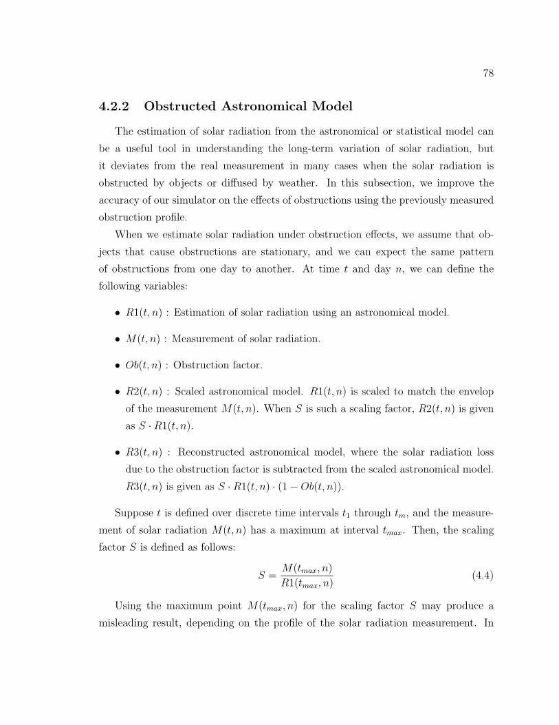
78

4.2.2 Obstructed Astronomical Model

The estimation of solar radiation from the astronomical or statistical model can

be a useful tool in understanding the long-term variation of solar radiation, but

it deviates from the real measurement in many cases when the solar radiation is

obstructed by objects or diffused by weather. In this subsection, we improve the

accuracy of our simulator on the effects of obstructions using the previously measured

obstruction profile.

When we estimate solar radiation under obstruction effects, we assume that ob-

jects that cause obstructions are stationary, and we can expect the same pattern

of obstructions from one day to another. At time t and day n, we can define the

following variables:

• R1(t, n) : Estimation of solar radiation using an astronomical model.

• M(t, n) : Measurement of solar radiation.

• Ob(t, n) : Obstruction factor.

• R2(t, n) : Scaled astronomical model. R1(t, n) is scaled to match the envelop

of the measurement M(t, n). When S is such a scaling factor, R2(t, n) is given

as S ·R1(t, n).

• R3(t, n) : Reconstructed astronomical model, where the solar radiation loss

due to the obstruction factor is subtracted from the scaled astronomical model.

R3(t, n) is given as S ·R1(t, n) · (1−Ob(t, n)).

Suppose t is defined over discrete time intervals t1 through tm, and the measure-

ment of solar radiation M(t, n) has a maximum at interval tmax. Then, the scaling

factor S is defined as follows:

S =M(tmax, n)

R1(tmax, n)(4.4)

Using the maximum point M(tmax, n) for the scaling factor S may produce a

misleading result, depending on the profile of the solar radiation measurement. In

79

order to remove the case when the maximum point is an outlier, we used a (100-

α/2)%-percentile point to calculate the scaling factor:

S =M(t(100−α/2)%max, n)

R1(t(100−α/2)%max, n)(4.5)

This removes outliers that exist outside (100 − α/2)% of the node distribution. For

example,

S =M(t97.5%max, n)

R1(t97.5%max, n)

is an scaling factor estimate that removes 5% of outliers.

The obstruction factor Ob(t, n) is the relative difference between the scaled astro-

nomical model R2(t, n) and the measurement M(t, n).

Ob(t, n) =

R2(t,n)−M(t,n)

R2(t,n)if R2(t, n) > 0,

1 otherwise.(4.6)

The reconstructed astronomical model at time t and date n′, R3(t, n′) is given

as S · R1(t, n′) · (1 − Ob(t, n′)). Since we assume that obstructions are stationary,

Ob(t, n′) = Ob(t, n). Thus,

R3(t, n′) = S ·R1(t, n′) · (1−Ob(t, n)) (4.7)

While the example above used samples from a single day to estimate the scaling

factor and the obstruction vector, estimates from multiple days can be used to reduce

the error. The process of creating a reconstructed astronomical model is summarized

in Figure 4.10.

Figure 4.11 shows the measurement M(t, n) with three different solar radiation

estimations: the astronomical model R1(t, n), the scaled astronomical model R2(t, n)

and the reconstructed astronomical model R3(t, n). A sensor node was placed in

a meadow under a tree, and we used the measurement gathered on 10/13/2007 to

calculate the scaling factor S and the obstruction factor Ob(t, n). Figure 4.12 com-

pares the solar radiation of different estimation methods with the measured value.

We can see that the reconstructed astronomical model R3(t, n) is very close to the

measurement M(t, n) when the weather is sunny. In Figure 4.12, the estimation error

of R3(t, n) is less than 25% on average.

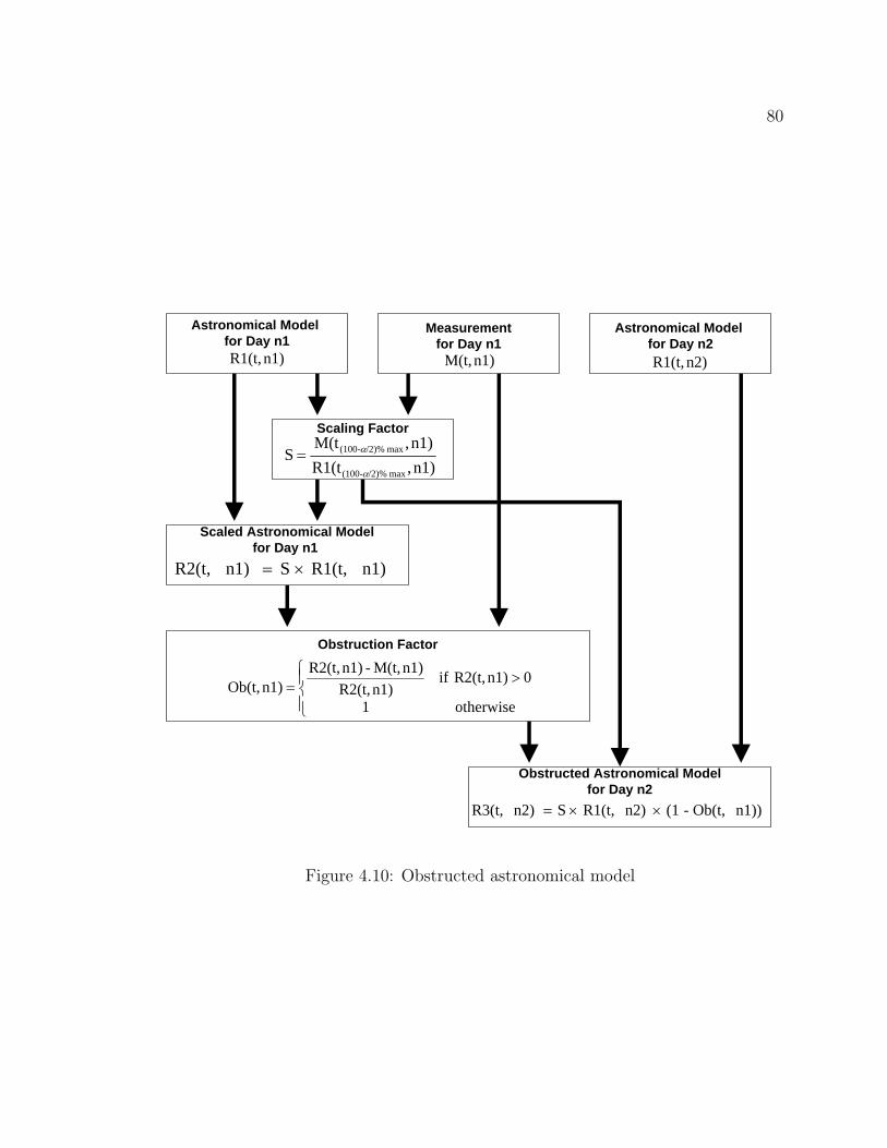
80

Scaling Factor

n1),R1(tn1),M(t

Smax /2)%(100-

max /2)%(100-

α

α=

Scaled Astronomical Modelfor Day n1

n1)R1(t,Sn1)R2(t, ×=

Obstructed Astronomical Modelfor Day n2

n1))Ob(t,-(1n2)R1(t,S n2)R3(t, ××=

Obstruction Factor

⎪⎩

⎪⎨⎧ >

=otherwise1

0n1) R2(t,ifn1)R2(t,

n1)M(t,-n1)R2(t,n1)Ob(t,

Astronomical Model for Day n2

n2)R1(t,

Measurementfor Day n1

n1)M(t,

Astronomical Model for Day n1

n1)R1(t,

Figure 4.10: Obstructed astronomical model

81

−5 0 5 10 15 20 250

50

100

150

200

250

Time of Day (Hour)

Pow

er (

mW

)

Router 78 − Daily Trend with n = 286, θp = 0, L = 37.87, φ

p = 180, τ = 0.1

SimulationScaled SimulationReconstructedMeasured − 10/13/07

Figure 4.11: Estimating the solar radiation using obstruction measurement

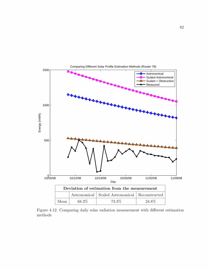
82

10/05/08 10/12/08 10/19/08 10/26/08 11/02/08 11/09/080

500

1000

1500

Day

Ene

rgy

(mW

h)

Comparing Different Solar Profile Estimation Methods (Router 78)

AstronomicalScaled AstronomicalScaled + ObstructionMeasured

Deviation of estimation from the measurement

Astronomical Scaled Astronomical Reconstructed

Mean 68.3% 73.3% 24.8%

Figure 4.12: Comparing daily solar radiation measurement with different estimationmethods

83

function[estimates, model] = get_IVcurve(xdata_V,ydata_mA,Isc_mA)start_point = rand(1, 2);model = @expfun;estimates = fminsearch(model, start_point);

function [sse, FittedCurve] = expfun(params)A = params(1);B = params(2);FittedCurve = Isc_mA - A .* ( exp(B * xdata_V) - 1);ErrorVector = FittedCurve - ydata_mA;sse = sum(ErrorVector .^ 2);

endend

Figure 4.13: Matlab algorithm for solar IV curve fitting

4.3 Modeling Solar Panel

4.3.1 Modeling IV Characteristic

The I-V characteristic of a solar panel can be described with a generic formula:

I = Isc − A · (exp(B · V )− 1) (4.8)

Having a generic formula allows us to determine the I-V characteristic of a solar cell

using the curve-fitting method, and the algorithm shown in Figure 4.13. As input

parameters, this algorithm takes a sequence of IV measurement points (xdata_V,

ydata_mA) and the short circuit current measurement Isc_mA. As a return value,

the algorithm returns a parameter pair (A, B) that minimizes the error between the

measured output and the estimated output. After the I-V characteristic of a solar

panel is determined, our model can find the current or power of a solar panel at a

given operational voltage (Figure 4.14). Figure 4.15 and 4.16 show IV characteristics

for two different types of solar panels. The first one is a 4V-100mA polycrystalline

silicon solar panel, and the second is a 3.6V-50mA amorphous silicon solar panel.

84

xdata_V = [0.23071.74402.54592.7926...4.21594.2224];

ydata_mA = [111.160109.800101.77096.910...9.1543.147];

Isc_mA = 111.16;

IV_params = get_IVcurve(xdata_V, ydata_mA, Isc_mA);

I_est_mA = Isc_mA - IV_params(1)*(exp(IV_params(2).* xdata_V)-1);P_est_mW = I_est_mA .* xdata_V;ydata_mW = ydata_mA .* xdata_V;

Figure 4.14: Matlab algorithm for estimating the solar panel IV and PV character-istics using measurement data. The units for voltage and current are V and mArespectively.

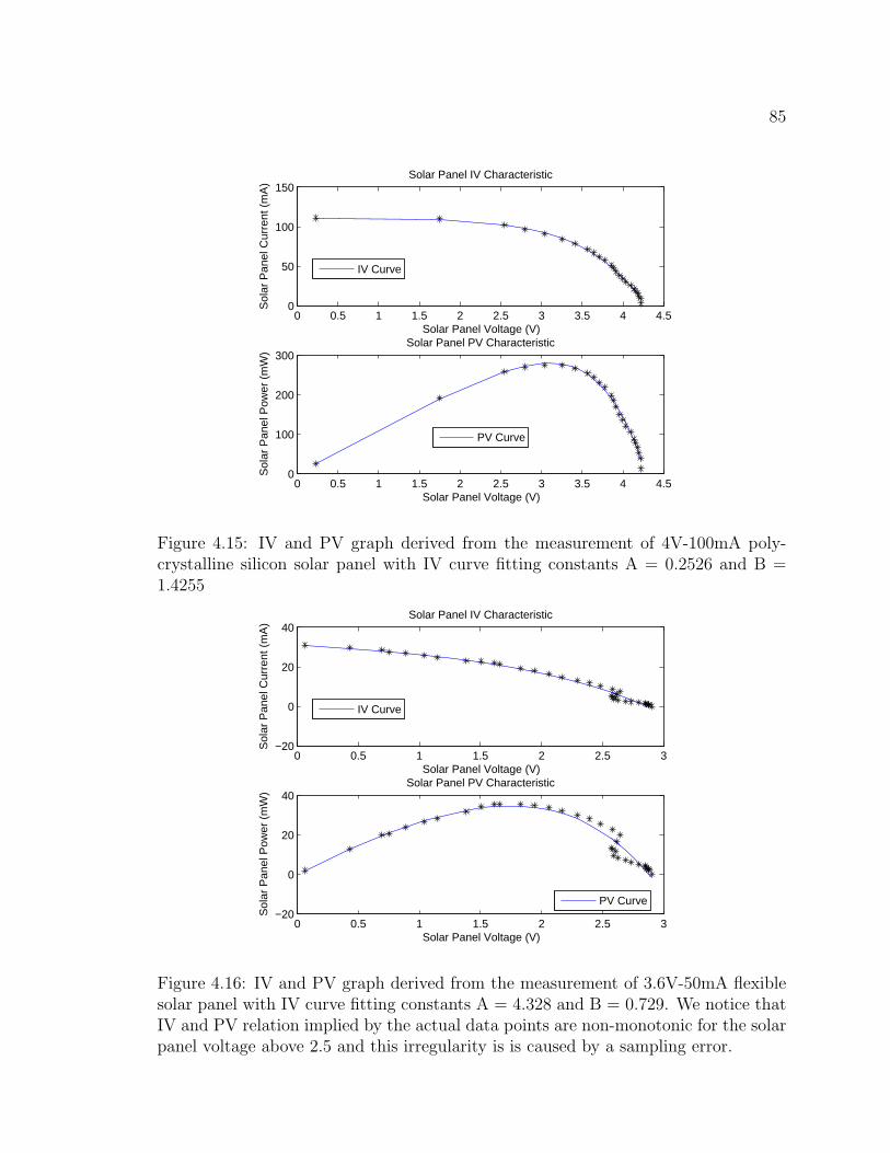
85

0 0.5 1 1.5 2 2.5 3 3.5 4 4.50

50

100

150


Sol

ar P

anel

Cur

rent

(m

A)


0 0.5 1 1.5 2 2.5 3 3.5 4 4.50

100

200

300


Sol

ar P

anel

Pow

er (

mW

)

Solar Panel PV Characteristic

IV Curve

PV Curve

Figure 4.15: IV and PV graph derived from the measurement of 4V-100mA poly-crystalline silicon solar panel with IV curve fitting constants A = 0.2526 and B =1.4255

0 0.5 1 1.5 2 2.5 3−20

0

20

40


Sol

ar P

anel

Cur

rent

(m

A)


IV Curve

0 0.5 1 1.5 2 2.5 3−20

0

20

40


Sol

ar P

anel

Pow

er (

mW

)


PV Curve

Figure 4.16: IV and PV graph derived from the measurement of 3.6V-50mA flexiblesolar panel with IV curve fitting constants A = 4.328 and B = 0.729. We notice thatIV and PV relation implied by the actual data points are non-monotonic for the solarpanel voltage above 2.5 and this irregularity is is caused by a sampling error.

86

4.3.2 Modeling the Operating Point

The solar panel operates as a voltage-controlled current source. The voltage of the

solar panel is determined by the output of the solar panel, which is either a battery

or a regulating diode.

Vpanel =

Vbatt + Vth−schottky with diode,

Vbatt otherwise.(4.9)

Once the voltage of the solar panel is determined, its current and power can be

determined by its IV curve.

4.4 Modeling Energy Storage

4.4.1 Modeling NiMH Rechargeable Battery

From the perspective of the micro-solar power simulator, NiMH rechargeable bat-

teries have two characteristics:

First, NiMH has different characteristics depending on whether it is in charging

mode or discharging mode, which makes the problem more complicated. This is

because the output voltage of the solar panel depends on the battery voltage, and the

battery can be either in charging mode or discharging mode, depending on the solar

panel output power. We address this problem by solving the states of all components

for a few possible modes and choosing the mode that meets the constraints of the

system. Figure 4.17 shows the capacity-to-voltage profiles for a NH15-2500 NiMH

battery.

Second, while a NiMH rechargeable battery maintains a stable voltage level for a

large operating range, its voltage level changes over the stored charge. This capacity-

to-voltage characteristic is non-linear and is not easily represented by a simple for-

mula. In order to represent this characteristic, we use the piecewise linear inter-

polation method, using the user-provided data for charging and discharging modes

(Figure 4.19).

Figure 4.18 describes an algorithm that evaluates the system state depending on

whether the battery is either in discharge or in charge. The system variables, initial

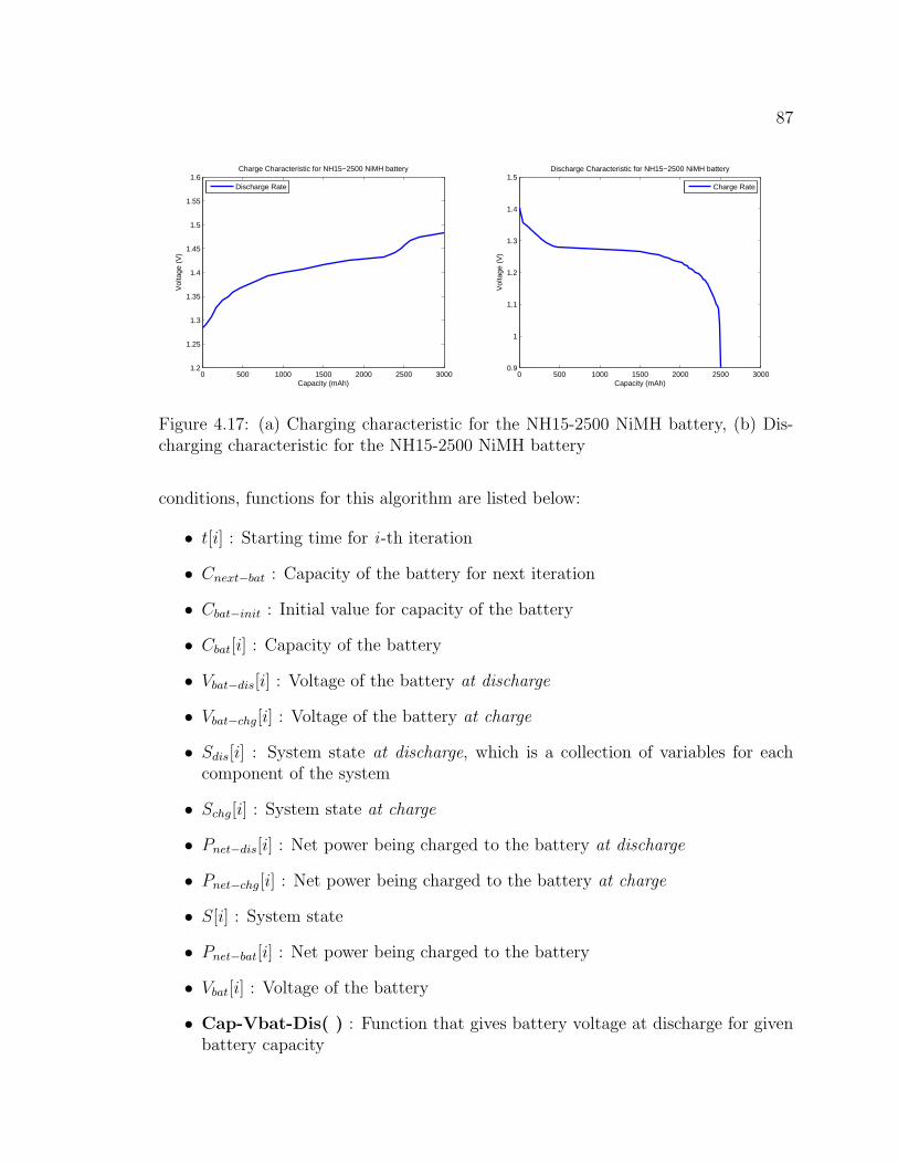
87

0 500 1000 1500 2000 2500 30001.2

1.25

1.3

1.35

1.4

1.45

1.5

1.55

1.6

Capacity (mAh)

Vol

tage

(V

)Charge Characteristic for NH15−2500 NiMH battery

Discharge Rate

0 500 1000 1500 2000 2500 30000.9

1

1.1

1.2

1.3

1.4

1.5

Capacity (mAh)

Vol

tage

(V

)

Discharge Characteristic for NH15−2500 NiMH battery

Charge Rate

Figure 4.17: (a) Charging characteristic for the NH15-2500 NiMH battery, (b) Dis-charging characteristic for the NH15-2500 NiMH battery

conditions, functions for this algorithm are listed below:

• t[i] : Starting time for i -th iteration

• Cnext−bat : Capacity of the battery for next iteration

• Cbat−init : Initial value for capacity of the battery

• Cbat[i] : Capacity of the battery

• Vbat−dis[i] : Voltage of the battery at discharge

• Vbat−chg[i] : Voltage of the battery at charge

• Sdis[i] : System state at discharge, which is a collection of variables for eachcomponent of the system

• Schg[i] : System state at charge

• Pnet−dis[i] : Net power being charged to the battery at discharge

• Pnet−chg[i] : Net power being charged to the battery at charge

• S[i] : System state

• Pnet−bat[i] : Net power being charged to the battery

• Vbat[i] : Voltage of the battery

• Cap-Vbat-Dis( ) : Function that gives battery voltage at discharge for givenbattery capacity

88

1: Cnext−bat ← Cbat−init

2: for i = 1 to N do

3: Cbat[i] ← Cnext−bat

4: Vbat−dis[i] ← Cap-Vbat-Dis(Cbat[i])

5: Vbat−chg[i] ← Cap-Vbat-Chg(Cbat[i])

6: Evaluate system state Sdis[i] at discharge using Vbat−dis[i].

7: Evaluate system state Schg[i] at charge using Vbat−chg[i].

8: Evaluate net battery charging power Pnet−dis[i] at discharge using Sdis[i].

9: Evaluate net battery charging power Pnet−chg[i] at charge using Schg[i].

10: if Pnet−dis > 0 ∨ Pnet−chg > 0 then

11: Set system state S[i] as Schg[i].

12: else

13: Set system state S[i] as Sdis[i].

14: end if

15: Cnext−bat ← Cbat[i] + (t[i+ 1]− t[i])× Pnet−bat[i]/Vbat[i]16: end for

Figure 4.18: Algorithm that evaluates the state of a micro-solar power system withNiMH battery

• Cap-Vbat-Chg( ) : Function that gives battery voltage at charge for given

battery capacity

4.4.2 Modeling Supercapacitors

For a given voltage level, the energy level of a supercapacitor can be calculated

using formula (4.10), and the voltage level can be calculated from the inverse equation:

E =1

2CV 2 ⇐⇒ V =

√2E

C(4.10)

Figure 4.20 shows the voltage-to-capacity relationship for a 22F supercapacitor.

89

function output_voltage = calc_vout_NH15_2500(capacity_mAh)

capacity = [0.0047.0093.75...2496.00];voltage = [1.4001.3551.345...0.900];N = max(size(capacity));if (capacity_mAh < capacity(1,1))

capacity_mAh = capacity(1,1);elseif (capacity_mAh > capacity(N,1))

capacity_mAh = capacity(N,1);endoutput_voltage = interp1(capacity, voltage, capacity_mAh);

Figure 4.19: Matlab algorithm for piecewise linear interpolation for the battery volt-age level over its capacity

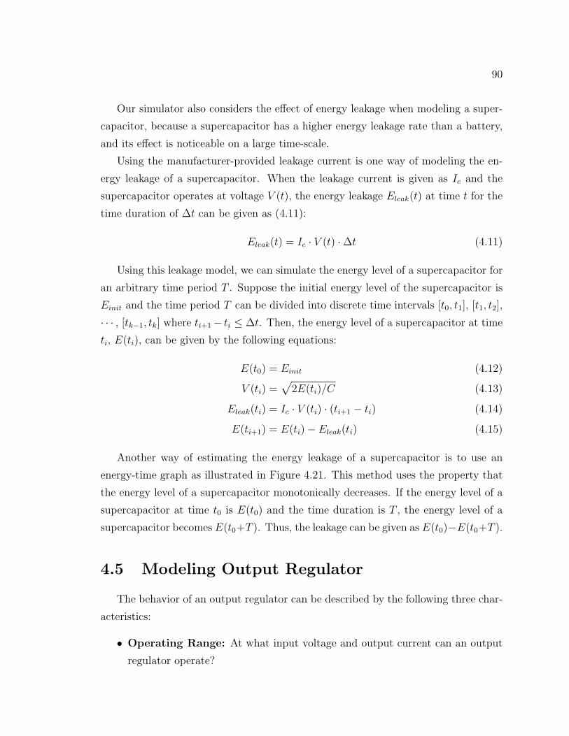
90

Our simulator also considers the effect of energy leakage when modeling a super-

capacitor, because a supercapacitor has a higher energy leakage rate than a battery,

and its effect is noticeable on a large time-scale.

Using the manufacturer-provided leakage current is one way of modeling the en-

ergy leakage of a supercapacitor. When the leakage current is given as Ic and the

supercapacitor operates at voltage V (t), the energy leakage Eleak(t) at time t for the

time duration of ∆t can be given as (4.11):

Eleak(t) = Ic · V (t) ·∆t (4.11)

Using this leakage model, we can simulate the energy level of a supercapacitor for

an arbitrary time period T . Suppose the initial energy level of the supercapacitor is

Einit and the time period T can be divided into discrete time intervals [t0, t1], [t1, t2],

· · · , [tk−1, tk] where ti+1− ti ≤ ∆t. Then, the energy level of a supercapacitor at time

ti, E(ti), can be given by the following equations:

E(t0) = Einit (4.12)

V (ti) =√

2E(ti)/C (4.13)

Eleak(ti) = Ic · V (ti) · (ti+1 − ti) (4.14)

E(ti+1) = E(ti)− Eleak(ti) (4.15)

Another way of estimating the energy leakage of a supercapacitor is to use an

energy-time graph as illustrated in Figure 4.21. This method uses the property that

the energy level of a supercapacitor monotonically decreases. If the energy level of a

supercapacitor at time t0 is E(t0) and the time duration is T , the energy level of a

supercapacitor becomes E(t0+T ). Thus, the leakage can be given as E(t0)−E(t0+T ).

4.5 Modeling Output Regulator

The behavior of an output regulator can be described by the following three char-

acteristics:

• Operating Range: At what input voltage and output current can an output

regulator operate?

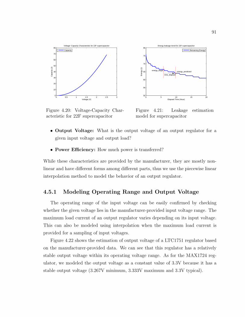
91

0 0.5 1 1.5 2 2.5 30

10

20

30

40

50

60

70

80

Voltage (V)

Cap

acity

(J)

Voltage−Capacity Characteristic for 22F supercapacitor

Capacity

Figure 4.20: Voltage-Capacity Char-acteristic for 22F supercapacitor

0 5 10 15 2050

55

60

65

70

75

80

Elapsed Time (Hour)

Ene

rgy

(J)

Energy leakage trend for 22F supercapacitor

Remaining Energy

energy_begin

time_elapsed

energy_predicted

Figure 4.21: Leakage estimationmodel for supercapacitor

• Output Voltage: What is the output voltage of an output regulator for a

given input voltage and output load?

• Power Efficiency: How much power is transferred?

While these characteristics are provided by the manufacturer, they are mostly non-

linear and have different forms among different parts, thus we use the piecewise linear

interpolation method to model the behavior of an output regulator.

4.5.1 Modeling Operating Range and Output Voltage

The operating range of the input voltage can be easily confirmed by checking

whether the given voltage lies in the manufacturer-provided input voltage range. The

maximum load current of an output regulator varies depending on its input voltage.

This can also be modeled using interpolation when the maximum load current is

provided for a sampling of input voltages.

Figure 4.22 shows the estimation of output voltage of a LTC1751 regulator based

on the manufacturer-provided data. We can see that this regulator has a relatively

stable output voltage within its operating voltage range. As for the MAX1724 reg-

ulator, we modeled the output voltage as a constant value of 3.3V because it has a

stable output voltage (3.267V minimum, 3.333V maximum and 3.3V typical).

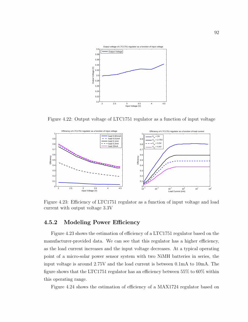
92

2 2.5 3 3.5 4 4.53.2

3.22

3.24

3.26

3.28

3.3

3.32

3.34

3.36

3.38

3.4

Input Voltage (V)

Out

put V

olta

ge (

V)

Output voltage of LTC1751 regulator as a function of input voltage

Output Voltage

Figure 4.22: Output voltage of LTC1751 regulator as a function of input voltage

2 2.5 3 3.5 4 4.50

0.1

0.2

0.3

0.4

0.5

0.6

0.7

0.8

0.9

1

Input Voltage (V)

Effi

cien

cy

Efficiency of LTC1751 regulator as a function of input voltage

load 0.001mAload 0.01mAload 0.1mAload 0.2mAload 20mA

10−3

10−2

10−1

100

101

102

0

0.1

0.2

0.3

0.4

0.5

0.6

0.7

0.8

0.9

1

Load Current (mA)

Effi

cien

cy

Efficiency of LTC1751 regulator as a function of load current

V

in = 2V

Vin

= 2.75V

Vin

= 3.3V

Vin

= 4.4V

Figure 4.23: Efficiency of LTC1751 regulator as a function of input voltage and loadcurrent with output voltage 3.3V

4.5.2 Modeling Power Efficiency

Figure 4.23 shows the estimation of efficiency of a LTC1751 regulator based on the

manufacturer-provided data. We can see that this regulator has a higher efficiency,

as the load current increases and the input voltage decreases. At a typical operating

point of a micro-solar power sensor system with two NiMH batteries in series, the

input voltage is around 2.75V and the load current is between 0.1mA to 10mA. The

figure shows that the LTC1751 regulator has an efficiency between 55% to 60% within

this operating range.

Figure 4.24 shows the estimation of efficiency of a MAX1724 regulator based on

93

1 1.5 2 2.5 3 3.5 4 4.5 50

0.1

0.2

0.3

0.4

0.5

0.6

0.7

0.8

0.9

1

Input Voltage (V)

Effi

cien

cy

Efficiency of MAX1724 regulator as a function of input voltage

load 0.01mAload 0.1mAload 1mAload 20mA

10−2

10−1

100

101

102

0.5

0.6

0.7

0.8

0.9

1

Load Current (mA)

Effi

cien

cy

Efficiency of MAX1724 regulator as a function of load current

V

in = 1.0V

Vin

= 1.5V

Vin

= 2.0V

Vin

= 2.5V

Figure 4.24: Efficiency of MAX1724 regulator as a function of input voltage and loadcurrent with output voltage 3.3V

the manufacturer-provided data. As is the case with the LTC1751, the efficiency of

the MAX1724 increases as the load current increases, but the voltage-to-efficiency of

the MAX1724 has a different characteristic from the LTC1751. As the input voltage

increases, the efficiency of the MAX1724 increases and it reaches the saturation point

at around 2.5V.

The MAX1724 regulator is more efficient than the LTC1751 regulator. To make

a fair comparison, we can look up the efficiency of the MAX1724 at the same in-

put voltage level (2.75V) and the load current range (0.1mA to 10mA). Figure 4.24

shows that the MAX1724 regulator has an efficiency between 75% to 80% within this

operating range. Whereas the efficiency of the LTC1751 is 55% to 60%.

4.6 Modeling the Input Regulator

4.6.1 Micro-Solar Power System without an Input Regulator

Before we model the input regulator, we can consider the behavior of a micro-solar

power system with no input regulator, as is illustrated in Figure 4.25. In this type of

micro-solar power system, the solar panel voltage Vsol is determined by the voltage

level of the energy storage, Vstor, and the threshold voltage of the diode, Vth−schottky,

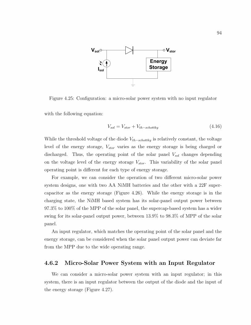
94

storsol

sol

Figure 4.25: Configuration: a micro-solar power system with no input regulator

with the following equation:

Vsol = Vstor + Vth−schottky (4.16)

While the threshold voltage of the diode Vth−schottky is relatively constant, the voltage

level of the energy storage, Vstor varies as the energy storage is being charged or

discharged. Thus, the operating point of the solar panel Vsol changes depending

on the voltage level of the energy storage Vstor. This variability of the solar panel

operating point is different for each type of energy storage.

For example, we can consider the operation of two different micro-solar power

system designs, one with two AA NiMH batteries and the other with a 22F super-

capacitor as the energy storage (Figure 4.26). While the energy storage is in the

charging state, the NiMH based system has its solar-panel output power between

97.3% to 100% of the MPP of the solar panel, the supercap-based system has a wider

swing for its solar-panel output power, between 13.9% to 98.3% of MPP of the solar

panel.

An input regulator, which matches the operating point of the solar panel and the

energy storage, can be considered when the solar panel output power can deviate far

from the MPP due to the wide operating range.

4.6.2 Micro-Solar Power System with an Input Regulator

We can consider a micro-solar power system with an input regulator; in this

system, there is an input regulator between the output of the diode and the input of

the energy storage (Figure 4.27).

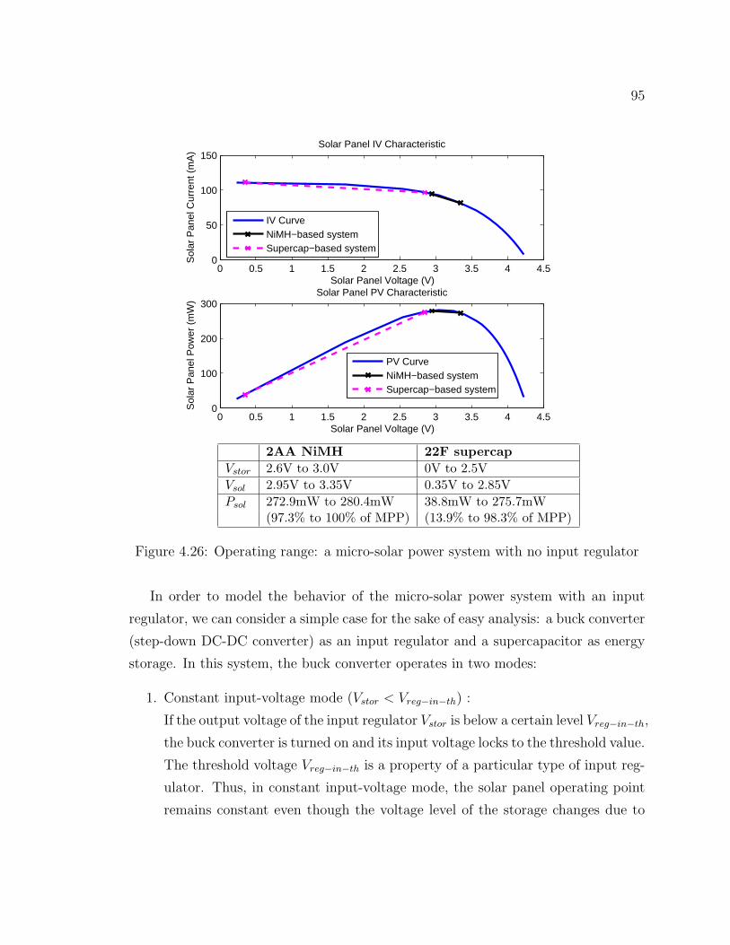
95

0 0.5 1 1.5 2 2.5 3 3.5 4 4.50

50

100

150


Sol

ar P

anel

Cur

rent

(m

A)


IV CurveNiMH−based systemSupercap−based system

0 0.5 1 1.5 2 2.5 3 3.5 4 4.50

100

200

300


Sol

ar P

anel

Pow

er (

mW

)


PV CurveNiMH−based systemSupercap−based system

2AA NiMH 22F supercapVstor 2.6V to 3.0V 0V to 2.5VVsol 2.95V to 3.35V 0.35V to 2.85VPsol 272.9mW to 280.4mW 38.8mW to 275.7mW

(97.3% to 100% of MPP) (13.9% to 98.3% of MPP)

Figure 4.26: Operating range: a micro-solar power system with no input regulator

In order to model the behavior of the micro-solar power system with an input

regulator, we can consider a simple case for the sake of easy analysis: a buck converter

(step-down DC-DC converter) as an input regulator and a supercapacitor as energy

storage. In this system, the buck converter operates in two modes:

1. Constant input-voltage mode (Vstor < Vreg−in−th) :

If the output voltage of the input regulator Vstor is below a certain level Vreg−in−th,

the buck converter is turned on and its input voltage locks to the threshold value.

The threshold voltage Vreg−in−th is a property of a particular type of input reg-

ulator. Thus, in constant input-voltage mode, the solar panel operating point

remains constant even though the voltage level of the storage changes due to

96

charge and discharge.

Vreg−in = Vth−reg−in = const (4.17)

Vsol = Vreg−in + Vth−schottky (4.18)

= Vth−reg−in + Vth−schottky = const

Isol = IV Curve(Vsol) = const (4.19)

2. Pass-through mode (Vstor > Vreg−in−th) :

If the output voltage of the input regulator Vstor is above the threshold Vreg−in−th,

the buck converter is turned off and looks like a pass-through wire from the out-

side. In pass-through mode, the solar panel operating point changes along the

solar panel IV curve, following the voltage of the storage.

Vreg−in = Vstor (4.20)

Vsol = Vreg−in + Vth−schottky (4.21)

= Vstor + Vth−schottky

Isol = IV Curve(Vsol) (4.22)

Figure 4.28 shows the case where a depleted supercapacitor is charged from a

solar panel through a buck converter. In the beginning, the voltage level of the

supercapacitor Vstor is low meeting the condition for the constant-input-voltage mode,

thus the buck converter is turned on and its input voltage Vreg−in becomes constant

due to the characteristic of constant input impedance of the device Rreg−in. Then,

the solar panel current also becomes constant.

As time goes on, the supercapacitor is charged and its voltage level Vstor rises.

When Vstor becomes high enough to meet the condition for the pass-through mode,

the buck converter is turned off and the solar panel voltage Vreg increases, following

the supercapacitor voltage Vstor. The solar panel voltage Vsol also increases as Vreg

increases. At the same time, the current of the solar panel Isol decreases along the

solar panel IV curve.

When the amount of energy that comes into the buck converter is given as Pin =

Vreg−in · Isol, the amount of energy that comes out of the buck converter can be given

as Pout = Effreg−in ·Pin. The power efficiency Effreg−in is provided by the manufacturer

and varies among parts.

97

storsol

sol

reg-in

Figure 4.27: Configuration: a micro-solar power system with a buck converter asan input regulator

Time

Vstor

(1) Vreg-in >= Vstor Time

Vsol

(2) Vreg-in < Vstor

Vreg-in-th

Figure 4.28: Operating range: a micro-solar power system with a buck converteras an input regulator

4.7 Modeling Load

4.7.1 Average Current-Based Model

For modeling the long-term behavior of the load, we can use the average current

consumption measured by a scope or a multimeter. This is because most sensornet

applications have periodic behavior of sensing and communication and any surge in

power consumption becomes averaged over a long period of time. In our simulator,

we use the average current-based model.

98

4.7.2 Application Code Based Model

For modeling the short-term behavior of the load, we can use a power consumption

simulator that takes application code. In the remainder of this subsection, we de-

scribe this methodology based on PowerTOSSIM [SHC+04], which is a representative

application-code-level power-consumption simulator.

Structure of PowerTOSSIM

Power profiling with PowerTOSSIM is done in three steps: application monitoring,

logging and post-processing (Figure 4.29). First, in the application monitoring step,

each TinyOS component that can influence the power consumption of a mote is

modified to call the power monitoring module PowerStateM through the PowerState

interface. Such TinyOS components are HPLADCC, PhotoTempM, CC1000ControlM,

LedsM, SnoozeM and EEPROMM. In the logging step, the power monitoring module

PowerStateM logs the power profile, such as component name, status and event time,

into an output file as the sensor component calls the power monitoring module. Lastly

in the post-processing step, the power status log file is associated with the power

consumption model for the mote platform to provide more meaningful results.

Extending PowerTOSSIM to a New Platform

Extending PowerTOSSIM beyond the reference platform requires changing pro-

gram code, as well as power consumption measurement for the power consumption

model. Even when the same program code is used, we may need new power consump-

tion measurement results because different hardware parts produce different power

consumption results (e.g. LedsM). The TinyOS modules in the reference implementa-

tion of PowerTOSSIM with the Mica2 platform can be divided into five categories: (1)

radio module, (2) LED module, (3) sensing module, (4) power management module

and (5) flash memory module.

As for the radio module, there is a platform dependency issue. The original Power-

TOSSIM is based on the CC1000 radio chip and the Atmel micro-controller, whereas

our reference platform, the HydroWatch node, runs on a different radio and micro-

controller: the CC2420 radio and MSP430 micro-controller. While we may write

99

a simulator module based on this reference platform, we decided not to for several

reasons.

First, TOSSIM requires the radio module communicate in bits, whereas the CC2420

radio is a packet-level radio. Thus, emulating CC2420 native code requires us to

change a major part of the TOSSIM simulator. Second, the applications that will

use the CC2420 radio need to access only the high-level interface, not the low-level

implementation details. Most CC2420 radio-based applications use the generic inter-

face. Although they need the CC2420 radio specific interface, they access only a small

number of functions, such as transmission power control. Thus, we have decided to

implement the simulator by writing a CC2420 radio wrapper module on top of the

simulator code for the CC1000 radio (Figure 4.30). The idea of using a wrapper

module provides the same programming interface to the applications that run on the

CC2420 radio, while minimizing the effort to write simulator code.

The LED module for PowerTOSSIM is quite straight-forward, but we corrected a

problem when we extended it for the TelosB platform. The original version of Pow-

erTOSSIM, built for the Mica2 platform, assumes the same power consumption for

three different types of LED. This is not the case for the TelosB mote (see RED LED,

GREEN LED and YELLOW LED in Table 4.2), and we corrected this problem by

making the post-processing script handle the current consumption for each LED dif-

ferently.

Other modules, such as sensing, power management and flash memory modules

aren’t yet implemented for the TelosB mote. But, this can be done in a straight-

forward way by identifying the TinyOS code that accesses these modules and building

the power consumption model for these modules from measurement.

In order to build the power consumption model for the TelosB node, we used two

instruments to measure the power consumption of a TelosB node: a Fluke-189 mul-

timeter and a Tektronics TDS7104 digital phosphor oscilloscope. The measurement

result is shown in Table 4.2.

Evaluating the Modified PowerTOSSIM

To evaluate the operation of PowerTOSSIM, we ran PowerTOSSIM for the TelosB

platform and compared it with the power consumption measured from a TelosB node

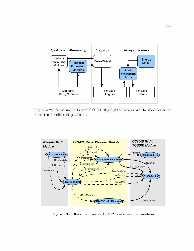
100

PostprocessingLoggingApplication Monitoring

PlatformIndependent

ModulesPlatform

DependentModules Post

processingScript

EnergyModel

PowerStateM

Application Being Monitored

SimulationLog File

SimulationResults

Figure 4.29: Structure of PowerTOSSIM. Highlighted blocks are the modules to berewritten for different platforms.

RadioCRCPacket

CC2420RadioC

CC2420RadioDummyM

CC2420ControlDummyM

RandomLFSR

CC1000RadioC

ReceiveMsg

StdControl

BareSendMsg

CC1000Control

CC2420Control

Random

StdControl

CC1000Control

SplitControl

MacControl

MacBackoff

RadioCoordinator

RadioCoordinator

BareSendMsg

StdControl

ReceiveMsg

CC1000 RadioTOSSIM Module

CC2420 Radio Wrapper ModuleGeneric RadioModule

Figure 4.30: Block diagram for CC2420 radio wrapper modules

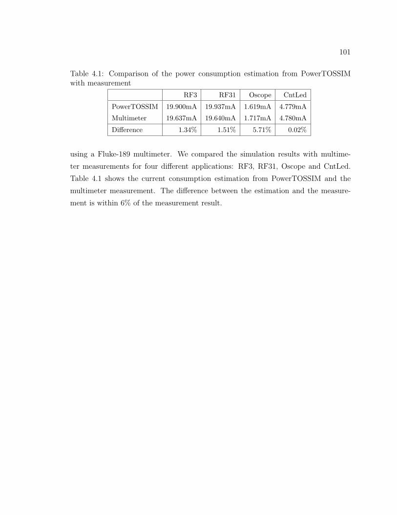
101

Table 4.1: Comparison of the power consumption estimation from PowerTOSSIMwith measurement

RF3 RF31 Oscope CntLed

PowerTOSSIM 19.900mA 19.937mA 1.619mA 4.779mA

Multimeter 19.637mA 19.640mA 1.717mA 4.780mA

Difference 1.34% 1.51% 5.71% 0.02%

using a Fluke-189 multimeter. We compared the simulation results with multime-

ter measurements for four different applications: RF3, RF31, Oscope and CntLed.

Table 4.1 shows the current consumption estimation from PowerTOSSIM and the

multimeter measurement. The difference between the estimation and the measure-

ment is within 6% of the measurement result.

102

Table 4.2: Power consumption model for TelosB node. The unit for each entity ismA except for VOLTAGE, the unit of which is V

Keyword Value Keyword Value

RADIO RX 19.405 VOLTAGE 3.0

RADIO OFF 0 CPU ACTIVE 1.986

RADIO TX 03 8.392 CPU IDLE 0.175

RADIO TX 04 8.956 CPU ADC NOISE REDUCTION 0.0

RADIO TX 05 9.040 CPU POWER DOWN 0.0

RADIO TX 06 9.081 CPU POWER SAVE 0.0

RADIO TX 07 9.452 CPU STANDBY 0.0037

RADIO TX 08 10.384 CPU EXTENDED STANDBY 0.0037

RADIO TX 09 10.277 CPU INIT 1.986

RADIO TX 0A 10.252 CPU FREQ 4000000

RADIO TX 0B 10.774 LED 2.2

RADIO TX 0C 11.388 LED INIT 0

RADIO TX 0D 11.448 RED LED 2.804

RADIO TX 0E 11.323 RED LED INIT 0

RADIO TX 0F 11.883 GREEN LED 4.461

RADIO TX 10 12.553 GREEN LED INIT 0

RADIO TX 11 12.578 YELLOW LED 2.002

RADIO TX 12 12.644 YELLOW LED INIT 0

RADIO TX 13 13.052 EEPROM READ 1.75

RADIO TX 14 13.596 EEPROM WRITE 2.69

RADIO TX 15 13.602 ADC 0.459

RADIO TX 16 13.572 SENSOR BOARD 0.69

RADIO TX 17 14.180 SENSOR PHOTO 0

RADIO TX 18 14.808 SENSOR TEMP 0

RADIO TX 19 14.859 SENSOR INTERNAL TEMP 0.332

RADIO TX 1A 14.828

RADIO TX 1B 15.388

RADIO TX 1C 15.911

RADIO TX 1D 15.861

RADIO TX 1E 15.929

RADIO TX 1F 16.442

RADIO DEFAULT POWER 31.00

103

4.8 Composition

In this section, we construct a model of the whole micro-solar power system and

simulate it based on the description of each component and its interconnection with

others. We simulate the model of a micro-solar power system in two steps: first,

under constant radiation, and second, under the daily solar radiation cycle.

4.8.1 Simulation under Constant Radiation

Here, we simulate the model of a micro-solar power system under constant radi-

ation using a controllable light source. This makes it easy to verify the simulation

model of the solar panel and the energy storage with the model of the external envi-

ronment set to the measurement data.

Effect of Input Regulator

We simulate the effect of an input regulator and verify it with the measurement.

• External Environment and Solar Panel: For a controlled external environ-

ment, we used an indoor lamp light to make the radiation constant throughout

the experiments. As for the solar panel, we used a 4.0V-100mA solar panel. The

IV and PV curves of the solar panel under this radiation condition are shown

in Figure 4.31.

• Input Regulator: We consider two cases. In the first case, no input regulator

is used where the output of the solar panel is directly connected to the energy

storage through a Schottky diode (Figure 4.25). In the second case, an LM3671

step-down DC-DC converter is used as an input regulator (Figure 4.27). The

LM3671 has a power efficiency between 80% and 90% within its operating range.

In simulating the LM3671, we assume an efficiency of 80%.

• Energy Storage: For the energy storage, we used a 22F supercapacitor from

Aerogel. We used a supercapacitor for this test because a supercapacitor has a

larger voltage swing (0V to 3V) from empty to full capacity than a recharge-

able battery such as a NiMH. This allowed us to test the system over a wider

operating range.

104

• Output Regulator and Load: Since this is to test the charging process of a

micro-solar power system, we did not use any output regulator or load.

The simulation and measurement result for the first case (not using an input

regulator) is shown in Figure 4.32. From this, we can draw the following observations:

1. As the supercapacitor is being charged, the solar panel voltage increases and

the solar panel current decreases. This is because the solar panel voltage follows

the supercap voltage, and the solar panel voltage and the solar-panel IV curve

determine the solar panel current. We can see that the simulation captures the

effect well.

2. From empty capacity (0.1V) to near-full capacity (2.9V), it took approximately

17 minutes in measurement and 20 minutes in simulation until the supercap

was fully charged.

3. The simulation closely predicts the behavior of the actual system. The corre-

lation coefficient and estimation error between the simulation result and the

measurement are shown in Figure 4.32. As for the supercapacitor voltage, the

correlation coefficient is 0.9904. The mean and the standard deviation of the

simulation error is -0.2376V and 0.1203V.

The simulation and measurement result for the second case (using an LM3671

step-down DC-DC converter as an input regulator) is shown in Figure 4.33. From

this, we can draw the following observations:

1. As the supercapacitor is being charged, the solar panel voltage and the solar

panel current change in two phases: first, the constant-input-voltage mode, and

second, the pass-through mode. We can see that the simulation captures this

two-phase operation well.

2. From empty capacity (0.1V) to near-full capacity (2.9V), it took approximately

19 minutes in measurement and 20 minutes in simulation until the supercapac-

itor was fully charged.

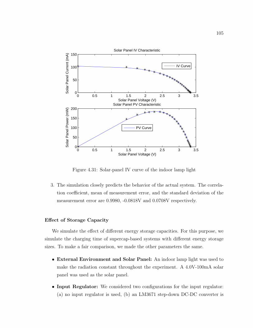
105

0 0.5 1 1.5 2 2.5 3 3.50

50

100

150


Sol

ar P

anel

Cur

rent

(m

A)


IV Curve

0 0.5 1 1.5 2 2.5 3 3.50

50

100

150

200


Sol

ar P

anel

Pow

er (

mW

)


PV Curve

Figure 4.31: Solar-panel IV curve of the indoor lamp light

3. The simulation closely predicts the behavior of the actual system. The correla-

tion coefficient, mean of measurement error, and the standard deviation of the

measurement error are 0.9980, -0.0818V and 0.0708V respectively.

Effect of Storage Capacity

We simulate the effect of different energy storage capacities. For this purpose, we

simulate the charging time of supercap-based systems with different energy storage

sizes. To make a fair comparison, we made the other parameters the same.

• External Environment and Solar Panel: An indoor lamp light was used to

make the radiation constant throughout the experiment. A 4.0V-100mA solar

panel was used as the solar panel.

• Input Regulator: We considered two configurations for the input regulator:

(a) no input regulator is used, (b) an LM3671 step-down DC-DC converter is

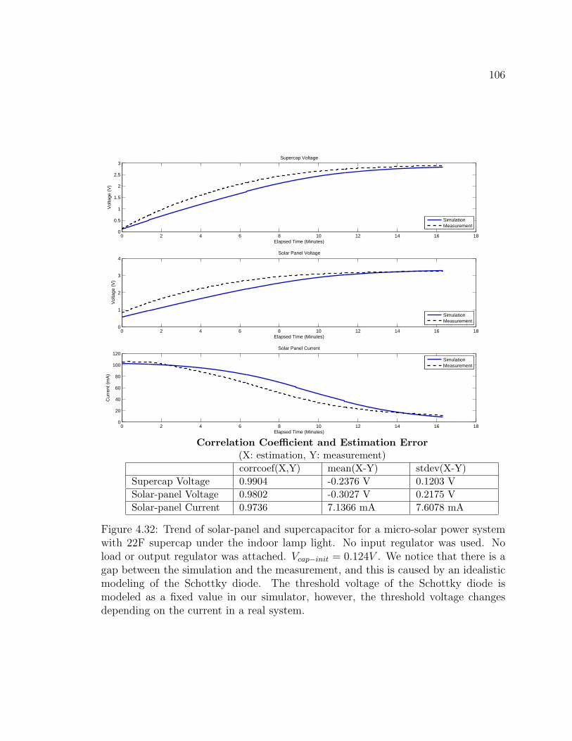
106

0 2 4 6 8 10 12 14 16 180

0.5

1

1.5

2

2.5

3

Elapsed Time (Minutes)

Vol

tage

(V

)

Supercap Voltage

SimulationMeasurement

0 2 4 6 8 10 12 14 16 180

1

2

3

4


Vol

tage

(V

)

Solar Panel Voltage


0 2 4 6 8 10 12 14 16 180

20

40

60

80

100

120


Cur

rent

(m

A)

Solar Panel Current


Correlation Coefficient and Estimation Error(X: estimation, Y: measurement)corrcoef(X,Y) mean(X-Y) stdev(X-Y)

Supercap Voltage 0.9904 -0.2376 V 0.1203 VSolar-panel Voltage 0.9802 -0.3027 V 0.2175 VSolar-panel Current 0.9736 7.1366 mA 7.6078 mA

Figure 4.32: Trend of solar-panel and supercapacitor for a micro-solar power systemwith 22F supercap under the indoor lamp light. No input regulator was used. Noload or output regulator was attached. Vcap−init = 0.124V . We notice that there is agap between the simulation and the measurement, and this is caused by an idealisticmodeling of the Schottky diode. The threshold voltage of the Schottky diode ismodeled as a fixed value in our simulator, however, the threshold voltage changesdepending on the current in a real system.

107

0 2 4 6 8 10 12 14 16 18 200

0.5

1

1.5

2

2.5

3


Vol

tage

(V

)

Supercap Voltage


0 2 4 6 8 10 12 14 16 18 200

1

2

3

4


Vol

tage

(V

)

Solar Panel Voltage


0 2 4 6 8 10 12 14 16 18 200

20

40

60

80

100

120


Cur

rent

(m

A)

Solar Panel Current



Supercap Voltage 0.9980 -0.0818 V 0.0708 VSolar-panel Voltage 0.9125 -0.0851 V 0.1098 VSolar-panel Current 0.9522 3.5611 mA 5.9328 mA

Figure 4.33: Trend of solar-panel and supercapacitor for a micro-solar power systemwith 22F supercap under the indoor lamp light. LM3671 step-down DC-DC converterwas used as an input regulator. No load or output regulator was attached. Vcap−init =0.130V .

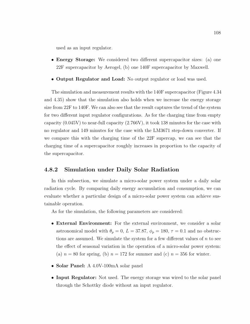
108

used as an input regulator.

• Energy Storage: We considered two different supercapacitor sizes: (a) one

22F supercapacitor by Aerogel, (b) one 140F supercapacitor by Maxwell.

• Output Regulator and Load: No output regulator or load was used.

The simulation and measurement results with the 140F supercapacitor (Figure 4.34

and 4.35) show that the simulation also holds when we increase the energy storage

size from 22F to 140F. We can also see that the result captures the trend of the system

for two different input regulator configurations. As for the charging time from empty

capacity (0.045V) to near-full capacity (2.766V), it took 138 minutes for the case with

no regulator and 149 minutes for the case with the LM3671 step-down converter. If

we compare this with the charging time of the 22F supercap, we can see that the

charging time of a supercapacitor roughly increases in proportion to the capacity of

the supercapacitor.

4.8.2 Simulation under Daily Solar Radiation

In this subsection, we simulate a micro-solar power system under a daily solar

radiation cycle. By comparing daily energy accumulation and consumption, we can

evaluate whether a particular design of a micro-solar power system can achieve sus-

tainable operation.

As for the simulation, the following parameters are considered:

• External Environment: For the external environment, we consider a solar

astronomical model with θp = 0, L = 37.87, φp = 180, τ = 0.1 and no obstruc-

tions are assumed. We simulate the system for a few different values of n to see

the effect of seasonal variation in the operation of a micro-solar power system:

(a) n = 80 for spring, (b) n = 172 for summer and (c) n = 356 for winter.

• Solar Panel: A 4.0V-100mA solar panel

• Input Regulator: Not used. The energy storage was wired to the solar panel

through the Schottky diode without an input regulator.

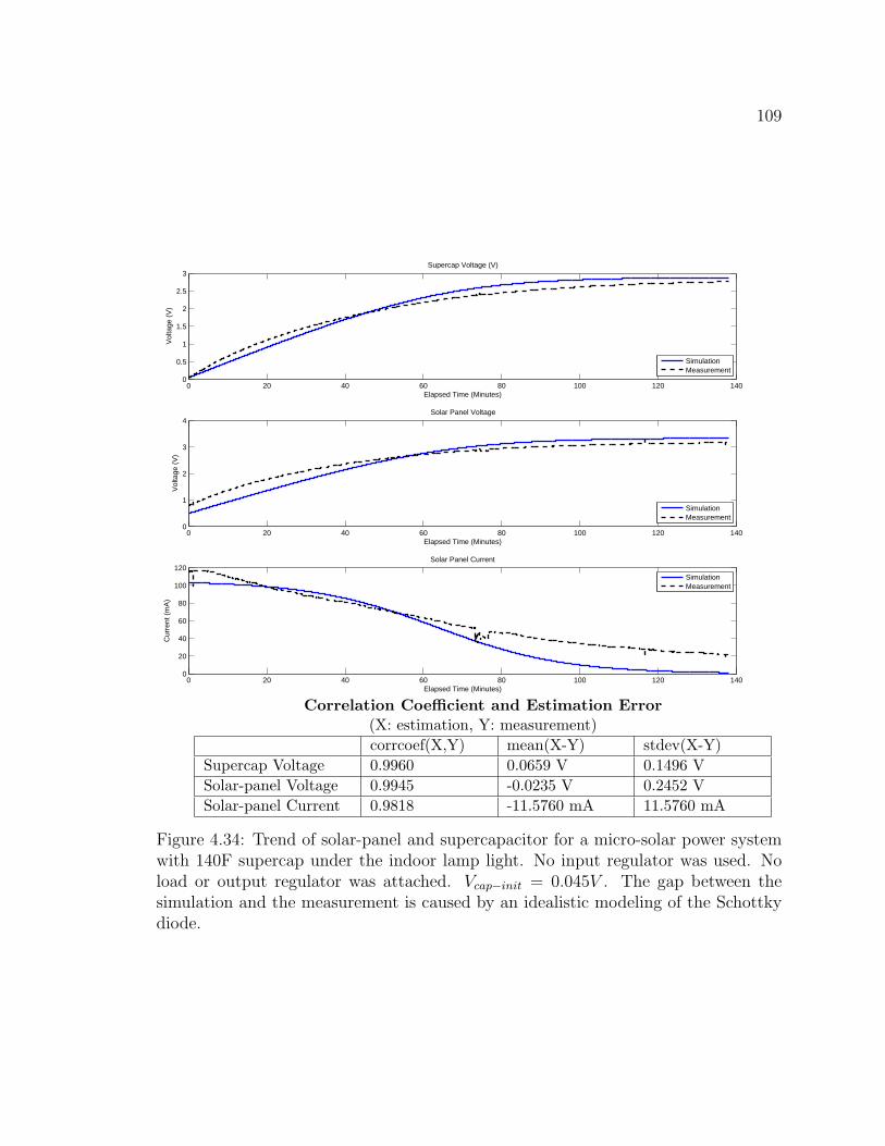
109

0 20 40 60 80 100 120 1400

0.5

1

1.5

2

2.5

3


Vol

tage

(V

)

Supercap Voltage (V)


0 20 40 60 80 100 120 1400

1

2

3

4


Vol

tage

(V

)

Solar Panel Voltage


0 20 40 60 80 100 120 1400

20

40

60

80

100

120


Cur

rent

(m

A)

Solar Panel Current



Supercap Voltage 0.9960 0.0659 V 0.1496 VSolar-panel Voltage 0.9945 -0.0235 V 0.2452 VSolar-panel Current 0.9818 -11.5760 mA 11.5760 mA

Figure 4.34: Trend of solar-panel and supercapacitor for a micro-solar power systemwith 140F supercap under the indoor lamp light. No input regulator was used. Noload or output regulator was attached. Vcap−init = 0.045V . The gap between thesimulation and the measurement is caused by an idealistic modeling of the Schottkydiode.

110

0 50 100 1500

0.5

1

1.5

2

2.5

3


Vol

tage

(V

)

Supercap Voltage (V)

0 50 100 1500

1

2

3

4


Vol

tage

(V

)

Solar Panel Voltage

0 50 100 1500

20

40

60

80

100

120


Cur

rent

(m

A)

Solar Panel Current





Supercap Voltage 0.9985 0.1736 V 0.0387 VSolar-panel Voltage 0.7036 0.0417 V 0.1387 VSolar-panel Current 0.9069 -9.6766 mA 9.2987 mA

Figure 4.35: Trend of solar-panel and supercapacitor for a micro-solar power systemwith 140F supercap under the indoor lamp light. LM3671 step-down DC-DC con-verter was used as an input regulator. No load or output regulator was attached.Vcap−init = 0.045V .

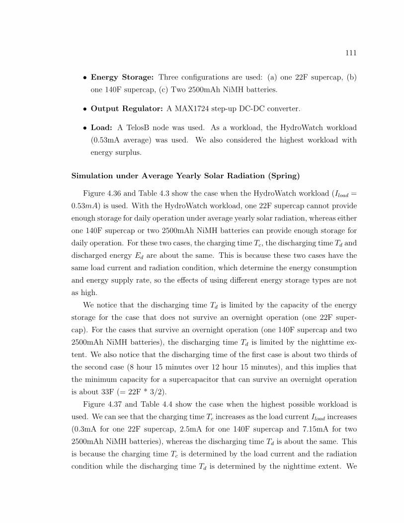
111

• Energy Storage: Three configurations are used: (a) one 22F supercap, (b)

one 140F supercap, (c) Two 2500mAh NiMH batteries.

• Output Regulator: A MAX1724 step-up DC-DC converter.

• Load: A TelosB node was used. As a workload, the HydroWatch workload

(0.53mA average) was used. We also considered the highest workload with

energy surplus.

Simulation under Average Yearly Solar Radiation (Spring)

Figure 4.36 and Table 4.3 show the case when the HydroWatch workload (Iload =

0.53mA) is used. With the HydroWatch workload, one 22F supercap cannot provide

enough storage for daily operation under average yearly solar radiation, whereas either

one 140F supercap or two 2500mAh NiMH batteries can provide enough storage for

daily operation. For these two cases, the charging time Tc, the discharging time Td and

discharged energy Ed are about the same. This is because these two cases have the

same load current and radiation condition, which determine the energy consumption

and energy supply rate, so the effects of using different energy storage types are not

as high.

We notice that the discharging time Td is limited by the capacity of the energy

storage for the case that does not survive an overnight operation (one 22F super-

cap). For the cases that survive an overnight operation (one 140F supercap and two

2500mAh NiMH batteries), the discharging time Td is limited by the nighttime ex-

tent. We also notice that the discharging time of the first case is about two thirds of

the second case (8 hour 15 minutes over 12 hour 15 minutes), and this implies that

the minimum capacity for a supercapacitor that can survive an overnight operation

is about 33F (= 22F * 3/2).

Figure 4.37 and Table 4.4 show the case when the highest possible workload is

used. We can see that the charging time Tc increases as the load current Iload increases

(0.3mA for one 22F supercap, 2.5mA for one 140F supercap and 7.15mA for two

2500mAh NiMH batteries), whereas the discharging time Td is about the same. This

is because the charging time Tc is determined by the load current and the radiation

condition while the discharging time Td is determined by the nighttime extent. We

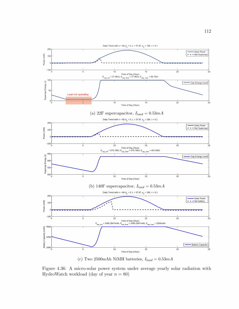
112

0 5 10 15 20 25−100

0

100

200

Time of Day (Hour)

Pow

er (m

W)

Daily Trend with n = 80, θp = 0, L = 37.87, φp = 180, τ = 0.1

Solar PanelNet Supercap

0 5 10 15 20 250

50

100

Time of Day (Hour)

Sup

erca

p E

nerg

y (J

)

Ecap_init = 27.983J, Ecap_final = 27.983J, Ecap_max = 68.750J

Cap Energy Level

5

Load not operating

(a) 22F supercapacitor, Iload = 0.53mA

0 5 10 15 20 25−100

0

100

200

Time of Day (Hour)

Pow

er (

mW

)

Daily Trend with n = 80, θp = 0, L = 37.87, φ

p = 180, τ = 0.1


0 5 10 15 20 25500

550

600

650

Time of Day (Hour)

Sup

erca

p E

nerg

y (J

)

Ecap_init

= 575.799J, Ecap_final

= 575.799J, Ecap_max

= 437.500J

Cap Energy Level

0 5 10 15 20 25

0

0.5

1

Time of Day (Hour)

0 to

1

Daily Trend with Imote

= 0.530mA

Load status

0 5 10 15 20 252.7

2.8

2.9

3

Time of Day (Hour)

Cap

Vol

(V

)

Vcap_init

= 2.868V, Vcap_max

= 2.500V, Vcap_final

= 2.868V

Supercap Voltage

(b) 140F supercapacitor, Iload = 0.53mA

0 5 10 15 20 25−100

0

100

200

Time of Day (Hour)

Pow

er (

mW

)


p = 180, τ = 0.1

Solar PanelNet battery

0 5 10 15 20 252490

2495

2500

Time of Day (Hour)

Bat

tery

Cap

acity

(m

Ah)

Ebat_init

= 2495.2847mAh, Ebat_final

= 2495.2847mAh, Ebat_max

= 2500mAh

Battery Capacity

0 5 10 15 20 25

0

0.5

1

Time of Day (Hour)

0 to

1


= 0.530mA

Load status

0 5 10 15 20 252.7

2.8

2.9

3

Time of Day (Hour)

Bat

Vol

(V

)

Vbat_init

= 2.7986V, Vbat_final

= 2.7986V

Battery Voltage

(c) Two 2500mAh NiMH batteries, Iload = 0.53mA

Figure 4.36: A micro-solar power system under average yearly solar radiation withHydroWatch workload (day of year n = 80)

113

Table 4.3: Simulation under average yearly solar radiation with HydroWatch workload(day of year n = 80).

Energy Storage One 22F super-cap

One 140F super-cap

Two 2500mAhNiMH batteries

Load CurrentIload

0.53 mA 0.53 mA 0.53 mA

Charging TimeTc

1 hour 45 minutes(06:15 to 08:00)

1 hour 30 minutes(06:15 to 07:45)

1 hour 45 minutes(06:15 to 08:00)

DischargingTime Td

8 hour 15 minutes(18:00 to 02:15)

12 hour 15 minutes(18:00 to 06:15)

12 hour 15 minutes(18:00 to 06:15)

Discharged En-ergy Ed

91.684J 110.238J 9.636mAh (=97.130J at 2.8V)

Table 4.4: Simulation under average yearly solar radiation with highest possible work-load (day of year n = 80)


One 140F super-cap


Load CurrentIload

0.30 mA 2.5 mA 7.15 mA

Charging TimeTc

1 hour 30 minutes(06:15 to 07:45)

3 hour 30 minutes(06:15 to 09:45)

5 hour 15 minutes(06:15 to 13:30)

DischargingTime Td

12 hour 30 min-utes (18:00 to06:15)

12 hour 30 minutes(17:45 to 06:15)

12 hour 45 minutes(17:30 to 06:15)


84.316J 493.798J 140.157mAh (=1412.8J at 2.8V)

also notice that the charging time does not increase linearly with the load current,

which is because the solar radiation is low at dawn and gets higher until noon.

Simulation under Worst-case of Yearly Solar Radiation (Winter)

Figure 4.38 and Table 4.5 show the case when the HydroWatch workload (Iload =

0.53mA) is used during winter (n = 356), which is the worst case for yearly solar

radiation. With the HydroWatch workload, one 22F supercap cannot provide enough

storage for daily operation under average yearly solar radiation, whereas, either one

140F supercap or two 2500mAh NiMH batteries can provide enough storage for daily

operation. For these two cases, we notice that the charging time and the discharging

time are longer than the case with average yearly solar radiation (n = 80), and this

is due to the fact that there is a smaller energy budget available during the winter.

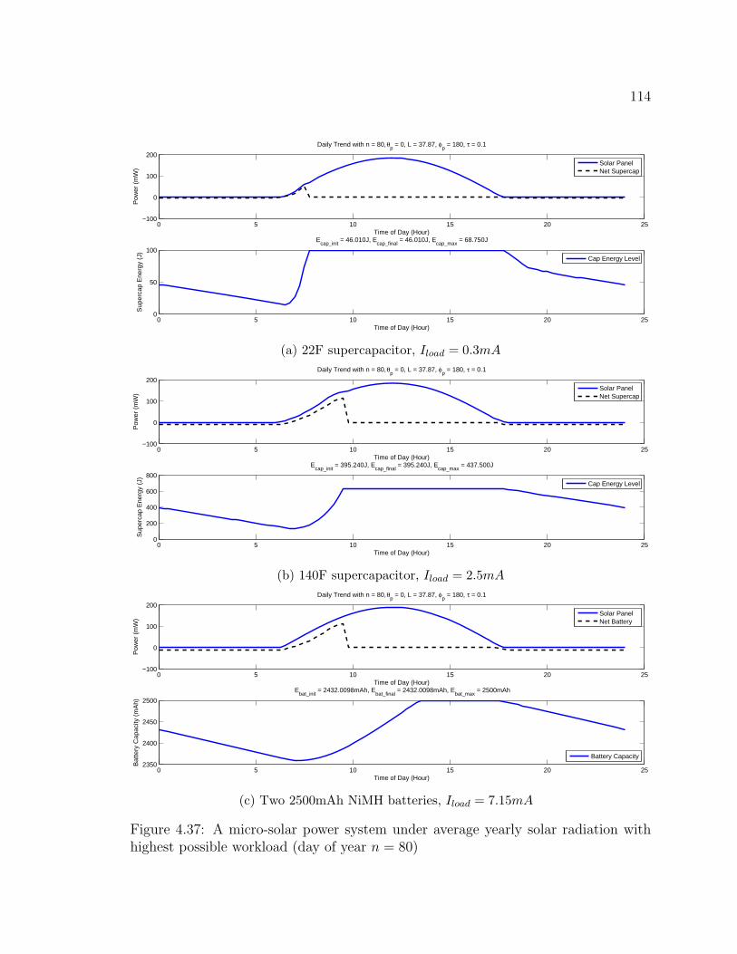
114

0 5 10 15 20 25−100

0

100

200

Time of Day (Hour)

Pow

er (

mW

)Daily Trend with n = 80, θ

p = 0, L = 37.87, φ

p = 180, τ = 0.1


0 5 10 15 20 250

50

100

Time of Day (Hour)

Sup

erca

p E

nerg

y (J

)

Ecap_init


= 46.010J, Ecap_max

= 68.750J

Cap Energy Level

0 5 10 15 20 25

0

0.5

1

Time of Day (Hour)

0 to

1


= 0.300mA

Load status

0 5 10 15 20 251

1.5

2

2.5

3

Time of Day (Hour)

Cap

Vol

(V

)

Vcap_init

= 2.045V, Vcap_max


= 2.045V

Supercap Voltage


0 5 10 15 20 25−100

0

100

200

Time of Day (Hour)

Pow

er (

mW

)


p = 180, τ = 0.1


0 5 10 15 20 250

200

400

600

800

Time of Day (Hour)

Sup

erca

p E

nerg

y (J

)

Ecap_init



= 437.500J

Cap Energy Level

0 5 10 15 20 25

0

0.5

1

Time of Day (Hour)

0 to

1


= 2.500mA

Load status

0 5 10 15 20 251

1.5

2

2.5

3

Time of Day (Hour)

Cap

Vol

(V

)

Vcap_init

= 2.376V, Vcap_max


= 2.376V

Supercap Voltage


0 5 10 15 20 25−100

0

100

200

Time of Day (Hour)

Pow

er (

mW

)


p = 180, τ = 0.1

Solar PanelNet Battery

0 5 10 15 20 252350

2400

2450

2500

Time of Day (Hour)

Bat

tery

Cap

acity

(m

Ah)

Ebat_init



= 2500mAh

Battery Capacity

0 5 10 15 20 25

0

0.5

1

Time of Day (Hour)

0 to

1


= 7.150mA

Load status

0 5 10 15 20 252.6

2.7

2.8

2.9

3

Time of Day (Hour)

Bat

Vol

(V

)

Vbat_init


= 2.7027V

Battery Voltage


Figure 4.37: A micro-solar power system under average yearly solar radiation withhighest possible workload (day of year n = 80)

115

0 5 10 15 20 25−50

0

50

100

150

Time of Day (Hour)

Pow

er (

mW


p = 0, L = 37.87, φ

p = 180, τ = 0.1


0 5 10 15 20 250

50

100

Time of Day (Hour)

Sup

erca

p E

nerg

y (J

)

Ecap_init


= 14.465J, Ecap_max

= 68.750J

Cap Energy Level

0 5 10 15 20 25

0

0.5

1

Time of Day (Hour)

0 to

1


= 0.530mA

Load status

0 5 10 15 20 250

1

2

3

Time of Day (Hour)

Cap

Vol

(V

)

Vcap_init

= 1.147V, Vcap_max


= 1.147V

Supercap Voltage


0 5 10 15 20 25−50

0

50

100

150

Time of Day (Hour)

Pow

er (

mW

)


p = 180, τ = 0.1


0 5 10 15 20 25450

500

550

600

650

Time of Day (Hour)

Sup

erca

p E

nerg

y (J

)

Ecap_init



= 437.500J

Cap Energy Level

0 5 10 15 20 25

0

0.5

1

Time of Day (Hour)

0 to

1


= 0.530mA

Load status

0 5 10 15 20 252.6

2.7

2.8

2.9

3

Time of Day (Hour)

Cap

Vol

(V

)

Vcap_init

= 2.837V, Vcap_max


= 2.837V

Supercap Voltage


0 5 10 15 20 25−50

0

50

100

150

Time of Day (Hour)

Pow

er (

mW

)


p = 180, τ = 0.1


0 5 10 15 20 252485

2490

2495

2500

Time of Day (Hour)

Bat

tery

Cap

acity

(m

Ah)

Ebat_init



= 2500mAh

Battery Capacity

0 5 10 15 20 25

0

0.5

1

Time of Day (Hour)

0 to

1


= 0.530mA

Load status

0 5 10 15 20 252.7

2.8

2.9

3

Time of Day (Hour)

Bat

Vol

(V

)

Vbat_init


= 2.7965V

Battery Voltage


Figure 4.38: A micro-solar power system under worst-case yearly solar radiation withHydroWatch workload (day of year n = 356)

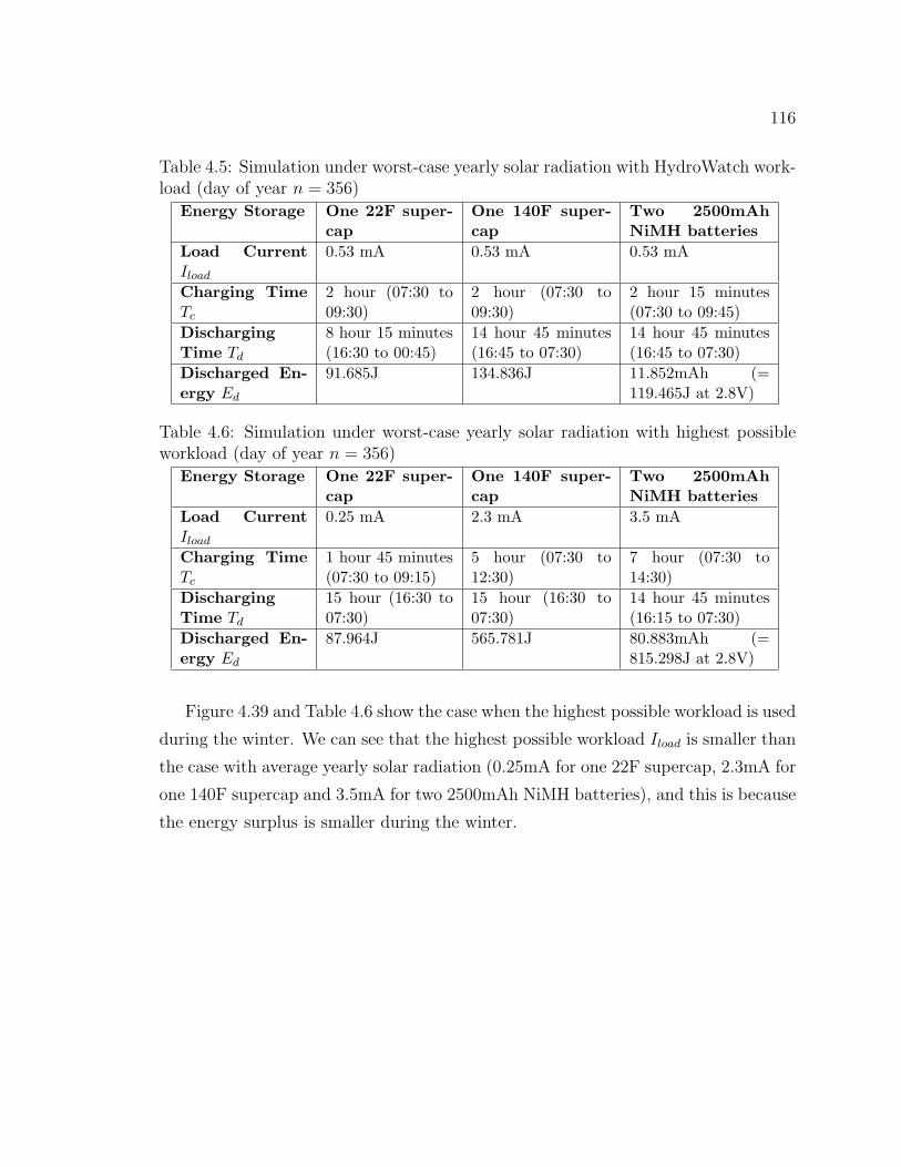
116

Table 4.5: Simulation under worst-case yearly solar radiation with HydroWatch work-load (day of year n = 356)


One 140F super-cap


Load CurrentIload

0.53 mA 0.53 mA 0.53 mA

Charging TimeTc

2 hour (07:30 to09:30)

2 hour (07:30 to09:30)

2 hour 15 minutes(07:30 to 09:45)

DischargingTime Td

8 hour 15 minutes(16:30 to 00:45)

14 hour 45 minutes(16:45 to 07:30)

14 hour 45 minutes(16:45 to 07:30)


91.685J 134.836J 11.852mAh (=119.465J at 2.8V)

Table 4.6: Simulation under worst-case yearly solar radiation with highest possibleworkload (day of year n = 356)


One 140F super-cap


Load CurrentIload

0.25 mA 2.3 mA 3.5 mA

Charging TimeTc

1 hour 45 minutes(07:30 to 09:15)

5 hour (07:30 to12:30)

7 hour (07:30 to14:30)

DischargingTime Td

15 hour (16:30 to07:30)

15 hour (16:30 to07:30)

14 hour 45 minutes(16:15 to 07:30)


87.964J 565.781J 80.883mAh (=815.298J at 2.8V)

Figure 4.39 and Table 4.6 show the case when the highest possible workload is used

during the winter. We can see that the highest possible workload Iload is smaller than

the case with average yearly solar radiation (0.25mA for one 22F supercap, 2.3mA for

one 140F supercap and 3.5mA for two 2500mAh NiMH batteries), and this is because

the energy surplus is smaller during the winter.

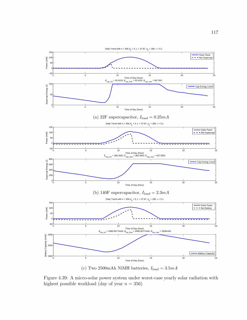
117

0 5 10 15 20 25−50

0

50

100

150

Time of Day (Hour)

Pow

er (

mW


p = 0, L = 37.87, φ

p = 180, τ = 0.1


0 5 10 15 20 250

50

100

Time of Day (Hour)

Sup

erca

p E

nerg

y (J

)

Ecap_init


= 43.419J, Ecap_max

= 68.750J

Cap Energy Level

0 5 10 15 20 25

0

0.5

1

Time of Day (Hour)

0 to

1


= 0.250mA

Load status

0 5 10 15 20 251

1.5

2

2.5

3

Time of Day (Hour)

Cap

Vol

(V

)

Vcap_init

= 1.987V, Vcap_max


= 1.987V

Supercap Voltage


0 5 10 15 20 25−50

0

50

100

150

Time of Day (Hour)

Pow

er (

mW

)


p = 180, τ = 0.1


0 5 10 15 20 250

200

400

600

800

Time of Day (Hour)

Sup

erca

p E

nerg

y (J

)

Ecap_init



= 437.500J

Cap Energy Level

0 5 10 15 20 25

0

0.5

1

Time of Day (Hour)

0 to

1


= 2.300mA

Load status

0 5 10 15 20 250

1

2

3

Time of Day (Hour)

Cap

Vol

(V

)

Vcap_init

= 2.285V, Vcap_max


= 2.285V

Supercap Voltage


0 5 10 15 20 25−50

0

50

100

150

Time of Day (Hour)

Pow

er (

mW

)


p = 180, τ = 0.1


0 5 10 15 20 252400

2450

2500

Time of Day (Hour)

Bat

tery

Cap

acity

(m

Ah)

Ebat_init



= 2500mAh

Battery Capacity

0 5 10 15 20 25

0

0.5

1

Time of Day (Hour)

0 to

1


= 3.500mA

Load status

0 5 10 15 20 252.6

2.7

2.8

2.9

3

Time of Day (Hour)

Bat

Vol

(V

)

Vbat_init


= 2.7323V

Battery Voltage


Figure 4.39: A micro-solar power system under worst-case yearly solar radiation withhighest possible workload (day of year n = 356)

118

4.9 Summary of Micro-Solar Power System Simu-

lator

In this chapter, we have presented a Mablab-based simulator of micro-solar power

systems. Below we summarize its architecture, principles and design methodology.

Overall Architecture and Principles

Our simulator is a time-event based simulator that has a modular architecture.

The simulator is composed of the six modules, each of which describes the corre-

sponding component in a micro-solar power system – external environment module,

solar panel module, input regulator module, energy storage module, output regulator

module and load module.

Our simulator has a modular and time-event architecture. First, our simulator

is designed in a modular way. The simulator is composed of the six modules, each

of which describes the corresponding component in a micro-solar power system –

external environment module, solar panel module, input regulator module, energy

storage module, output regulator module and load module. With the simulator, a

hypothetical system can be composed by plugging these modules together. Second,

our simulator is a time-event based simulator. The daily behavior is simulated by

iteratively evaluating the state of a system for the given initial condition and the time

interval vector, and similarly, the long-term behavior is simulated by iteratively evalu-

ating the daily behavior. Third, our simulator defines each module either analytically

or empirically depending on the availability of the well-defined characteristic.

Modeling Solar Radiation

Our simulator provides two ways to model solar radiation. An astronomical model,

which estimates solar radiation by calculating the angle between the sunlight and the

normal to the sunlight, is used when the weather is clear and the solar panel is not

obstructed. However, its estimation becomes significantly different from the actual

measurement under obstruction. An obstructed astronomical model, which is a re-

finement of the astronomical model, can estimate solar radiation with relatively high

119

accuracy even under obstruction using an empirical measurement on previous days.

The obstructed astronomical model is based on the following two assumptions: first,

the estimation from the astronomical model bounds the envelope of the solar radiation

measurement; second, nodes and local obstruction objects are stationary, and the ob-

struction pattern changes little over days. From the first assumption, the obstructed

astronomical model calculates an obstruction factor by taking a linear difference of

the measurement and the estimation of the astronomical model on a relatively clear

day n1. From the second assumption, the model estimates the solar radiation on

a different day n2 by multiplying the obstruction factor with the estimation of the

astronomical model on n2.

Modeling Solar Panel

Our simulator models the behavior of a solar panel in two steps: first it defines

the I-V characteristic of a panel; then it determines the operating point of the panel

in a whole system. The simulator models the I-V characteristic of a solar panel with

a generic curve I = Isc − A · (exp(B · V ) − 1) and instantiates the generic curve

into a specific curve using a Matlab curve-fitting algorithm when a sequence of (I, V )

measurement points are given. The simulator sets the operating voltage of the solar

panel in a whole system as the voltage of the output of the solar panel using the fact

that the solar panel operates as a voltage-controlled current source. Once the voltage

of the solar panel is determined, its current and power can be determined by its I-V

curve.

Modeling Energy Storage

Our simulator models two types of energy storage that are widely used for micro-

solar power systems: a NiMH battery and a supercapacitor. In order to simulate the

behavior of these two types of energy storage, our simulate models capacity-to-voltage

relation, charge-and-discharge relation, and self-discharge effect.

Capacity-to-voltage relation: For the case of a NiMH battery, the simulator models

capacity-to-voltage relation using a manufacturer-provided capacity-to-voltage graph.

Since a NiMH battery has different characteristics for the charging mode and the

discharging mode, the simulator models its capacity-to-voltage relation differently

120

depending on whether the system is in the charging mode or not. For the case of a

supercapacitor, the simulator models capacity-to-voltage relation using a well-known

formula, E = 12CV 2. Unlike a NiMH battery, a supercapacitor has the same operating

mode for charging and discharging.

Charge-and-discharge relation: At each time interval, the simulator estimates en-

ergy increment, which tells how much energy is charged into or discharged from the

energy storage during the time interval. At the end of a time interval, this increment

is added to the current energy level of the energy storage. In the next iteration, the

voltage level of the energy storage is evaluated from the updated energy level using

the capacity-to-voltage relation.

Self-discharge effect : Our simulator models the self-discharge effect for a super-

capacitor, which has a high leakage rate compared to its energy capacity. The self-

discharge effect is modeled either analytically with a manufacturer-provided leakage

current or empirically with an energy-time graph.

Modeling Output Regulator

Our simulator models the behavior of an output regulator using a piecewise-linear

interpolation method. This is because it is difficult to describe the behavior of vari-

ous types of output regulator in a simple formula: their characteristics are different

depending on the underlying technology and their behaviors are non-linear. For the

given input voltage and the output current, the simulator determines the output volt-

age and the power efficiency by interpolating them from the pre-measured data points

– either from a manufacturer-provided data sheet or from empirical measurement.

Modeling Input Regulator

Our simulator models two different configurations for an input regulator. The

first configuration is when the solar panel is connected to the energy storage through

a Schottky diode without an input regulator being used, and it is modeled by setting

the voltage of the solar panel as the voltage of the energy storage offseted by the

threshold voltage of the Schottky diode. In this configuration, the voltage of the

solar panel follows the voltage of the energy storage. The second configuration is

when the solar panel is connected to the energy storage through a buck converter,

121

and it is modeled in a two-mode operation. In constant input voltage mode where

the voltage of the energy storage is below a certain threshold, the input voltage of

the input regulator stays constant and the voltage of the solar panel becomes also

constant. In pass-through mode where the voltage of the energy storage is above the

threshold, the input voltage of the input regulator becomes equal to the voltage of

the energy storage. As the energy storage is being charged or discharged, the voltage

of the solar panel follows the voltage of the energy storage.

Modeling Load

For modeling the power consumption of the load, we have introduced two meth-

ods: an average current based model and an application code based model. An

average current based model, which is used in our simulator, abstracts the behavior

of the load as average current consumption. It is suitable for modeling the long term

behavior because most sensornet applications have periodic behavior of sensing and

communication, and any surge in power consumption becomes averaged over a long

period of time. An application code based model estimates the power consumption

of the load over varying time using a source-level simulator and a power consumption

look-up table. Since the time scale of this method can be as small as the timer interval

of the simulator, it is suitable for modeling a short-term behavior of the load.

Composition

Using the component models described above, we have composed and simulated

several designs of micro-solar power systems varying the following parameters: solar

radiation, input regulator type, energy storage type and energy storage capacity. The

simulation fits well with the measurement from actual implementations of micro-

solar power systems, and this shows that our simulator can estimate the behavior

of different variations of micro-solar power system quite effectively with sufficient

accuracy.

122

Chapter 5

Validating the Simulator Design

Using a Reference Implementation

The simulation becomes meaningful only after it is supported by reality. We have

shown its accuracy in controlled settings in the lab. In this chapter, the simulation

model of micro-solar power systems developed in the previous chapter is validated in

realistic outdoor experiments using a reference implementation. This chapter first de-

scribes the reference implementation of a micro-solar power system, the HydroWatch

node, in Section 5.1 focusing on its key design ideas. Then, in Section 5.2, it validates

the simulation model using energy flow measurements taken from urban neighborhood

and forest watershed deployments.

5.1 Node and Network Design of Reference Imple-

mentation

The HydroWatch Project [Unia] aims to collect widespread, high-frequency, and

automated observations of the life cycle of water as it progresses through a for-

est ecosystem. To gather this data, we aimed to deploy a robust network of low-

maintenance sensor nodes that could collect scientifically-relevant data indefinitely,

while withstanding a challenging wet forest environment. This section details the net-

work architecture, node mechanical design, and micro-power solar subsystem present

on each node.

123

Figure 5.1: System architecture for the HydroWatch micro-climate network.

5.1.1 Network Architecture

The sensor network architecture follows the canonical habitat monitoring form de-

scribed in [SOP+04], but is somewhat of a second-generation sensor network utilizing

several commercially available elements. The sensor node is built around the TelosB-

compatible Tmote Sky [Sen], and is described in detail below. The mote software,

which provides periodic data acquisition, thresholding, power management, remote

command processing, and health monitoring, is a modified Primer Pack/IP [Arc]

based on TinyOS 2.0. The patch network is an implementation of IPv6 using 6LoW-

PAN over IEEE 802.15.4 radios [MKHC07]. It utilizes a packet-based form of low-

power listening [PHC04] to minimize idle listening. Data collection is implemented as

UDP packets with the routing layer using hop-by-hop retransmissions and dynamic

rerouting in a redundant mesh (up to three potential parents) to provide path reli-

ability on lossy links. It utilizes Trickle-based [LPCS04] route updates for topology

maintenance. Source-based IPv6 routing is used to communicate directly to specific

nodes and dissemination is performed as a series of IPv6 link-local broadcasts.

In the initial HydroWatch deployment at the Angelo Reserve in Northern Cal-

ifornia, the sensor patch contained 19 nodes over a 220m x 260m area stretching

across a deep ravine formed by Elder Creek, up the deeply forested north slope of

124

the watershed area, and bending to the east to a particular tall stand of Douglas Fir

trees.

The transit network between the base-station and the patch was implemented

using the same node and link technology as the patch, so there is no specific gateway

node in the patch. To provide redundancy in the transit network, multiple micro-

solar router nodes cover a 120m stretch from a shed housing the gateway across an old

apple orchard. These nodes are just patch nodes without the environmental sensors.

The network depth is 5 hops or greater. The IEEE 802.15.4 bridge node attached

to the base-station uses a high-gain (19 dBi) parabolic antenna pointed out through

a window in the shed. The back haul network is a WiFi-based IP network with

repeaters on peaks and tree tops to reach a T1 line.

The base-station is a Linux-class gateway server that provides a web services front-

end, a PostgreSQL database for information storage and retrieval, and a web-based

management console. It is also an IP router, permitting end-to-end connectivity to

the patch nodes. The server facilitates such tasks as monitoring overall network health

remotely, diagnosing misreporting or missing nodes, and checking the quality of links

a node has to its neighbors, a function which proved critically important during the

deployment phase.

The initial physical deployment of this architecture is illustrated in Figure 5.2. The

base-station appears at the left (west) side of the image. The router nodes form a

sparse stretch reaching southeast, and a fairly rich interconnection is provided among

the several nodes up the watershed. Node sites were chosen to achieve both vertical

(up the hill) and horizontal (across the hill) profiles to enable an initial understanding

of the micro-climates in the watershed.

5.1.2 Engineering the Node

While the mote platform (micro-controller, radio, and flash), system software,

and networking are fairly common across many applications, the sensor suite, power

subsystem, and mechanical design of the node tend to be application-specific and

highly interrelated.

The sensor suite for this micro-climate monitoring application was essentially de-

veloped for tracking weather fronts in Redwoods [TPS+05] and available natively on

125

Figure 5.2: Snapshot of the HydroWatch forest watershed deployment.

Temp / RH Sensor

TSR, PAR Sensor Solar Panel

Antenna HydroSolar Board

TelosB Mote

NiMH Battery

Enclosure

Figure 5.3: HydroWatch weather node.

126

the TelosB platform – total solar radiation (TSR), photosynthetically active radia-

tion (PAR), temperature, and relative humidity. However, to provide high-quality

data, the sensors must be exposed properly to the environment while the rest of the

electronics are protected. We used the TelosB-compatible Tmote Sky mote [PSC05]

with an attached SMA connector for an external antenna and no on-board sensors.

We connected the mote to external sensor boards using custom cables with IDC con-

nectors, providing a degree of freedom to determine sensor orientation on the node.

The two photo-diodes used to measure incident PAR (Hamamatsu S1087) and

TSR (Hamamatsu S1087-01) are tiny discs connected to two long leg-like contacts.

Previous experience [TPS+05] recommends that these sensors should be elevated from

their surroundings to avoid collecting water on the sensing surface and to obtain

unobstructed indications of solar illumination.

A Sensirion SHT15 sensor measures relative humidity (RH) and temperature,

factory calibrated to exhibit a maximum +/- 2% RH and +/- 0.3 degrees Celsius

error. To accurately measure humidity requires the sensor be exposed to naturally-

aspirated air flow, whereas to measure temperature it should be shaded and decoupled

from large thermal masses and sources of self-heating. To meet these demands, the

SHT15 was placed within a 2-in PVC cap and suspended from the underside of the

node. To prevent electrical malfunction, the hole in the top of the PVC cap for the

interface wire was sealed and conformal coating was applied to the sensor board.

Though we recognize that a hanging design may be prone to connection disturbances

caused by curious wildlife, the accuracy of sensor data was worth the risk of a small

number of unavailable nodes.

The RF environment was expected to pose a critical challenge for our network,

due to interactions of foliage and water vapor with 2.4 GHz radio connectivity. Evi-

dent from past deployments [SMP+04,LBV06,WAJR+05,ZSLM04,DHJ+06] and more

specifically forest deployments [TPS+05,COSKM05], natural environments are capa-

ble of eliciting tremendous swings in link quality, causing wireless networks to fail

drastically and unexpectedly. To address this issue, we provisioned our nodes with

a 7 dBi omnidirectional antenna with a flexible orientation. Nodes were attached to

the top of 3 ft and 4 ft metal fence posts by a simple angle bracket.

Overall, the mechanical design of the node sought to provide accurate sensor

127

readings over a long duration. To protect the internal electronic components from

environmental damage, we limited the number of node features that required holes

in the enclosure; every opening in the enclosure is a potential opportunity for a leak.

Additionally, packets of indicating desiccant were placed inside each enclosure box,

preventing water vapor from damaging interior electronic components.

5.1.3 Micro-Solar Power Subsystem of HydroWatch Node

The core of the node design is a flexible power subsystem board that ties together

a solar panel, an optional input regulator, a battery, and a switching output regulator

– as shown in Figure 5.4. It provides measurement points for a number of electrical

parameters that can be connected to the mote ADCs, sampled and recorded along

with the environmental measurements. In our configuration, these monitoring fea-

tures produce time-series logs of solar panel voltage, solar panel current, and battery

voltage, in addition to the logs of sensor data from the application and link/neighbor

data. All of these are collected and stored by the gateway server, enabling deeper

analysis of the performance of the node and network under varying solar conditions.

The solar board also provides the mechanical structure that attaches the mote to the

enclosure.

The HydroWatch board was designed to permit the study of a variety of power

subsystem options. The solar panel and the battery are attached through screw

terminals. Headers and mounting holes permit direct attachment of motes of the

TelosB form factor, but a mote of any other type can be attached to the board

through screw terminals. Additionally, the board has a prototyping area which can

be used to change power subsystem configuration. In fact, we were able to change

any of the circuit elements originally used in the board schematic by simply changing

jumper settings and populating the prototyping area. We used this flexibility to

evaluate candidate parts for each component and quantify their contribution to the

efficiency of the entire system.

This section provides the rationale and key criteria for selecting specific compo-

nents as seen through the lens of our experience designing the HydroWatch board.

We begin with an analysis of application load – this directly impacts the selection

of the other components in the design. The components ultimately selected for the

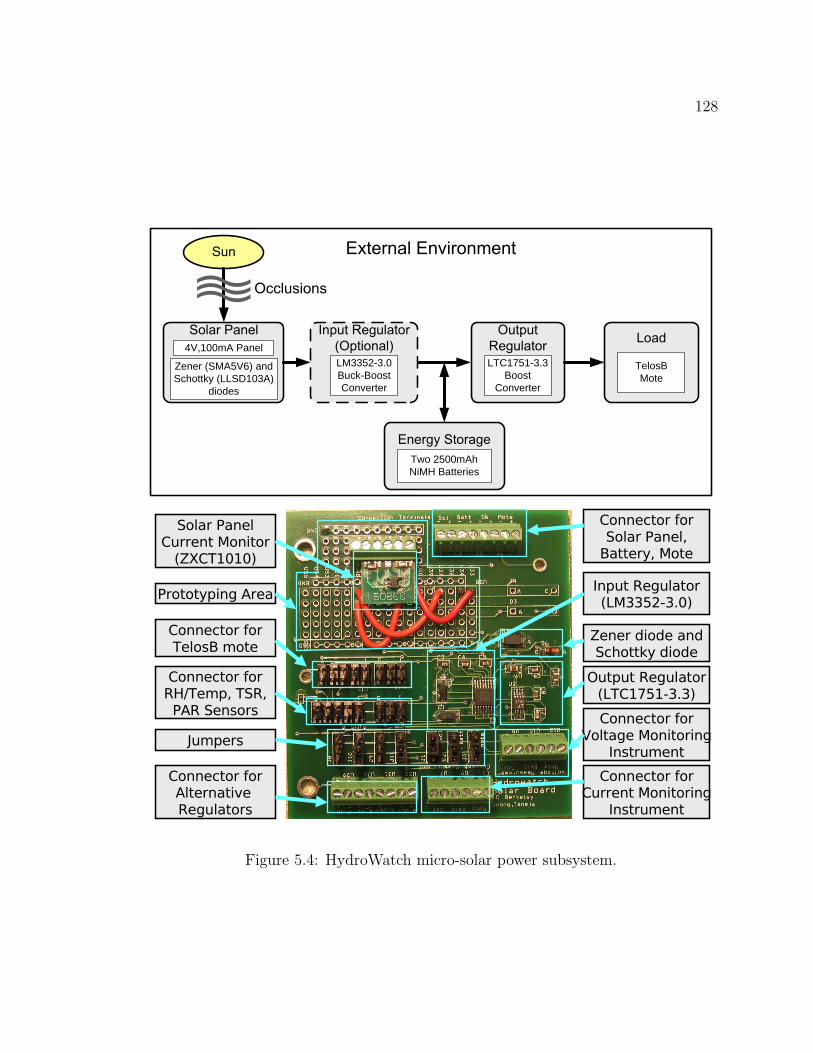
128

Two 2500mAhNiMH Batteries

LTC1751-3.3Boost

Converter

TelosBMote

4V,100mA Panel

Zener (SMA5V6) andSchottky (LLSD103A)

diodes

LM3352-3.0Buck-Boost Converter

Input Regulator(LM3352-3.0)

Connector forSolar Panel,

Battery, Mote

Output Regulator(LTC1751-3.3)

Solar PanelCurrent Monitor

(ZXCT1010)

Prototyping Area

Connector forTelosB mote

Connector forRH/Temp, TSR,PAR Sensors

Connector forVoltage Monitoring

Instrument

Connector forCurrent Monitoring

Instrument

Jumpers

Connector forAlternative Regulators

Zener diode andSchottky diode

Figure 5.4: HydroWatch micro-solar power subsystem.

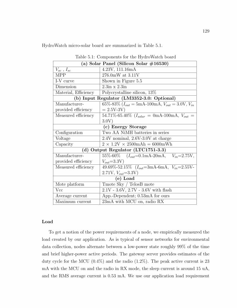
129

HydroWatch micro-solar board are summarized in Table 5.1.

Table 5.1: Components for the HydroWatch board

(a) Solar Panel (Silicon Solar #16530)Voc , Isc 4.23V, 111.16mAMPP 276.0mW at 3.11VI-V curve Shown in Figure 5.5Dimension 2.3in x 2.3inMaterial, Efficiency Polycrystalline silicon, 13%

(b) Input Regulator (LM3352-3.0: Optional)Manufacturer-provided efficiency

65%-83% (Iout = 5mA-100mA, Vout = 3.0V, Vin= 2.5V-3V)

Measured efficiency 54.71%-65.40% (Isolar = 0mA-100mA, Vout =3.0V)(c) Energy Storage

Configuration Two AA NiMH batteries in seriesVoltage 2.4V nominal, 2.6V-3.0V at chargeCapacity 2 × 1.2V × 2500mAh = 6000mWh

(d) Output Regulator (LTC1751-3.3)Manufacturer-provided efficiency

55%-60% (Iout=0.1mA-20mA, Vin=2.75V,Vout=3.3V)

Measured efficiency 49.69%-52.15% (Iout=3mA-6mA, Vin=2.55V-2.71V, Vout=3.3V)

(e) LoadMote platform Tmote Sky / TelosB moteVcc 2.1V - 3.6V, 2.7V - 3.6V with flashAverage current App.-Dependent; 0.53mA for oursMaximum current 23mA with MCU on, radio RX

Load

To get a notion of the power requirements of a node, we empirically measured the

load created by our application. As is typical of sensor networks for environmental

data collection, nodes alternate between a low-power state roughly 99% of the time

and brief higher-power active periods. The gateway server provides estimates of the

duty cycle for the MCU (0.4%) and the radio (1.2%). The peak active current is 23

mA with the MCU on and the radio in RX mode, the sleep current is around 15 uA,

and the RMS average current is 0.53 mA. We use our application load requirement

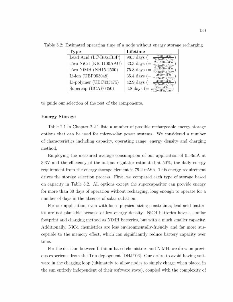
130

Table 5.2: Estimated operating time of a node without energy storage recharging

Type Lifetime

Lead Acid (LC-R061R3P) 98.5 days (= 7800mWh79.2mWh/day

)

Two NiCd (KR-1100AAU) 33.3 days (= 2×1320mWh79.2mWh/day

)

Two NiMH (NH15-2500) 75.8 days (= 2×3000mWh79.2mWh/day

)

Li-ion (UBP053048) 35.4 days (= 2800mWh79.2mWh/day

)

Li-polymer (UBC433475) 42.9 days (= 3400mWh79.2mWh/day

)

Supercap (BCAP0350) 3.8 days (= 304mWh79.2mWh/day

)

to guide our selection of the rest of the components.

Energy Storage

Table 2.1 in Chapter 2.2.1 lists a number of possible rechargeable energy storage

options that can be used for micro-solar power systems. We considered a number

of characteristics including capacity, operating range, energy density and charging

method.

Employing the measured average consumption of our application of 0.53mA at

3.3V and the efficiency of the output regulator estimated at 50%, the daily energy

requirement from the energy storage element is 79.2 mWh. This energy requirement

drives the storage selection process. First, we compared each type of storage based

on capacity in Table 5.2. All options except the supercapacitor can provide energy

for more than 30 days of operation without recharging, long enough to operate for a

number of days in the absence of solar radiation.

For our application, even with loose physical sizing constraints, lead-acid batter-

ies are not plausible because of low energy density. NiCd batteries have a similar

footprint and charging method as NiMH batteries, but with a much smaller capacity.

Additionally, NiCd chemistries are less environmentally-friendly and far more sus-

ceptible to the memory effect, which can significantly reduce battery capacity over

time.

For the decision between Lithium-based chemistries and NiMH, we drew on previ-

ous experience from the Trio deployment [DHJ+06]. Our desire to avoid having soft-

ware in the charging loop (ultimately to allow nodes to simply charge when placed in

the sun entirely independent of their software state), coupled with the complexity of

131

integrating a hardware Li-ion charger, dictated the selection of NiMH, as it operates

with more straightforward charging logic. This choice does present some drawbacks,

however. This chemistry suffers from a self-discharge rate of 30% per month and an

input-output efficiency of roughly 66%, both worse than for any other battery chem-

istry considered. The practical implication of this is that for every 3 units of energy

that are input to a battery, only 2 units of energy are output. We felt this cost was

overcome by the simplicity of the charging logic.

A 2-cell configuration would enable the potential to operate without an input

regulator; this choice is further discussed later in this section. For increased capacity,

it would be possible to put 2-cell packs in parallel. Additionally, since the discharge

curve of NiMH batteries is relatively flat, most of the discharge cycle produces a

near-constant voltage.

Solar Panel

In selecting an appropriate panel for a micro-solar subsystem, the critical factors

are the panel’s IV curve (specifically, the MPP), its cell composition, and its physical

dimensions. Care should be taken in selecting a panel that will operate near its MPP

given the load it is expected to support, be it a combination of an input regulator

and energy storage or energy storage alone. The cell composition – that is, how many

cells are present and their serial/parallel arrangement – becomes a factor when the

solar panel is partially occluded. Last, the physical dimensions of the panel should

be compatible for the choice of enclosure.

For the HydroWatch power subsystem, we selected a 4V-100mA panel from Silicon

Solar Inc., whose characteristics are summarized in Table 5.1(a) and whose IV and

PV curves are in Figure 5.5. The MPP of this panel occurs at 3.11V, which makes it

appropriate for charging 2 NiMH cells directly. Additionally, using our rule of thumb

of 30 minutes of sunlight per day, the solar energy generated by this panel at its MPP

is 139 mWh, satisfying the 120 mWh (= 79.2 mWh / 66% NiMH charge-discharge

efficiency) per day requirement of our application.

132

0 0.5 1 1.5 2 2.5 3 3.5 4 4.50

20

40

60

80

100

120

Solar Cell Voltage (V)

Sol

ar C

ell O

utpu

t Cur

rent

(mA

)

HydroSolar Node Solar Panel Characteristic at 10/13/2007 11:50AM

InterpolationMeasurement

0 0.5 1 1.5 2 2.5 3 3.5 4 4.50

50

100

150

200

250

300

Solar Cell Voltage (V)

Sol

ar C

ell O

utpu

t Pow

er (

mW

)

HydroSolar Node Solar Panel Characteristic at 10/13/2007 11:50AM

P−V CurveMPP (3.11V, 276.0mW)With input−regulator (measured)Without input−regulator (measured)With input−regulator (estimated)Without input−regulator (estimated)

Figure 5.5: Current-Voltage and Power-Voltage performance of the Silicon Solar 4V-100mA solar panel.

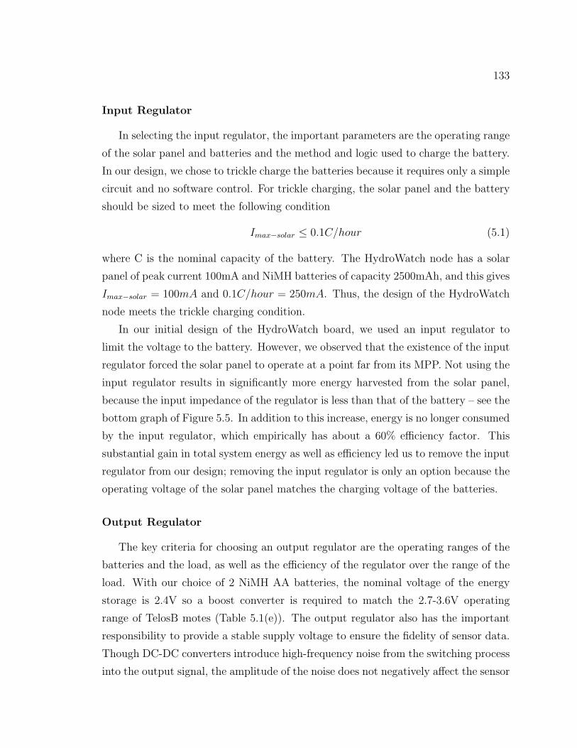
133

Input Regulator

In selecting the input regulator, the important parameters are the operating range

of the solar panel and batteries and the method and logic used to charge the battery.

In our design, we chose to trickle charge the batteries because it requires only a simple

circuit and no software control. For trickle charging, the solar panel and the battery

should be sized to meet the following condition

Imax−solar ≤ 0.1C/hour (5.1)

where C is the nominal capacity of the battery. The HydroWatch node has a solar

panel of peak current 100mA and NiMH batteries of capacity 2500mAh, and this gives

Imax−solar = 100mA and 0.1C/hour = 250mA. Thus, the design of the HydroWatch

node meets the trickle charging condition.

In our initial design of the HydroWatch board, we used an input regulator to

limit the voltage to the battery. However, we observed that the existence of the input

regulator forced the solar panel to operate at a point far from its MPP. Not using the

input regulator results in significantly more energy harvested from the solar panel,

because the input impedance of the regulator is less than that of the battery – see the

bottom graph of Figure 5.5. In addition to this increase, energy is no longer consumed

by the input regulator, which empirically has about a 60% efficiency factor. This

substantial gain in total system energy as well as efficiency led us to remove the input

regulator from our design; removing the input regulator is only an option because the

operating voltage of the solar panel matches the charging voltage of the batteries.

Output Regulator

The key criteria for choosing an output regulator are the operating ranges of the

batteries and the load, as well as the efficiency of the regulator over the range of the

load. With our choice of 2 NiMH AA batteries, the nominal voltage of the energy

storage is 2.4V so a boost converter is required to match the 2.7-3.6V operating

range of TelosB motes (Table 5.1(e)). The output regulator also has the important

responsibility to provide a stable supply voltage to ensure the fidelity of sensor data.

Though DC-DC converters introduce high-frequency noise from the switching process

into the output signal, the amplitude of the noise does not negatively affect the sensor

134

readings. If noise were a critical factor, either a low-pass filter or a higher voltage

energy supply in combination with a linear drop out (LDO) regulator could be used

instead. We chose the LTC1751 regulator [Tec], which had an efficiency of around

50%. It requires very few discrete parts and has low, constant switching noise.

5.1.4 Modeling the HydroWatch node for the Simulator

Based on the methodology described in Chapter 4, we modeled the operation of

the HydroWatch node as follows:

• External Environment: As for the external environment, we considered three

models: the astronomical model, scaled astronomical model and obstructed

astronomical model.

• Solar Collector: We used a 4V-100mA polycrystalline solar panel. We mod-

eled the solar panel using a generic form of I-V characteristic:

I = Isc − A · (exp(B · V )− 1) (5.2)

where Isc is the short circuit current of the solar panel and A and B are

the panel-specific constants. Using the curve-fitting method discussed in Sec-

tion 4.3.1, we have determined these constants as Isc = 111.160, A = 0.2526

and B = 1.4255.

• Input Regulator: The HydroWatch node has no input regulator. The solar

panel voltage Vsol is determined by the voltage level of the energy storage Vstor

and the threshold voltage of the diode Vth−schottky with the following equation:

Vsol = Vstor + Vth−schottky (5.3)

The threshold voltage of the diode Vth−schottky is modeled as a single value 0.45V,

which is taken as an average for a number of possible current draws for the diode.

• Energy Storage: A HydroWatch node uses two 2500mAh NiMH battery as

its energy storage. In order to model the capacity of a NiMH battery, we used

a battery capacity-to-voltage graph taken from the manufacturer provided data

(Figure 4.17).

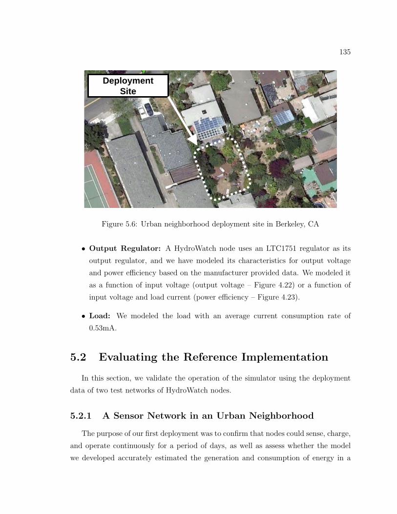
135

DeploymentSite

Figure 5.6: Urban neighborhood deployment site in Berkeley, CA

• Output Regulator: A HydroWatch node uses an LTC1751 regulator as its

output regulator, and we have modeled its characteristics for output voltage

and power efficiency based on the manufacturer provided data. We modeled it

as a function of input voltage (output voltage – Figure 4.22) or a function of

input voltage and load current (power efficiency – Figure 4.23).

• Load: We modeled the load with an average current consumption rate of

0.53mA.

5.2 Evaluating the Reference Implementation

In this section, we validate the operation of the simulator using the deployment

data of two test networks of HydroWatch nodes.

5.2.1 A Sensor Network in an Urban Neighborhood

The purpose of our first deployment was to confirm that nodes could sense, charge,

and operate continuously for a period of days, as well as assess whether the model

we developed accurately estimated the generation and consumption of energy in a

136

10/07/07 10/08/07 10/09/070

200

400

600

800

1000

1200

1400

1600

1800

2000

Day

Dai

ly S

olar

Ene

rgy

Rec

eive

d (m

Whr

)

Daily Solar Energy Measurements in Berkeley, CA

Node 12Node 06Node 03Mote Consumption

01/00/00 01/01/000

1.67

3.34

5.01

6.68

8.35

10.02

11.69

13.36

15.03

16.7

Sur

plus

Bat

tery

Day

s

Figure 5.7: Scatter plot of solar energy received in the urban neighborhood deploy-ment. Three representative nodes are highlighted.

variety of solar conditions. We deployed 22 nodes in an urban neighborhood in

Berkeley; nodes were placed in varied locations, including on a house gutter, in and

under trees, among shrubbery, and in a grassy yard. To emulate the situation in the

forest watershed, we placed them in the vicinity of significant obstructions and varied

the orientation of the solar panels: some were flat while others faced south, east, and

west at a 45 degree inclination.

Overall Trend

The range of daily solar energy via Psol by each node over a period of three days

can be seen in Figure 5.7. The lines on the graph show the behavior of the node that

received the highest (Node 12), median (Node 06), and lowest (Node 03) amount of

solar energy. The fourth line on the graph shows a constant 79.2 mWh break-even

point. The first day (10/07/2007) was a fairly sunny day, resulting in the widest

distribution of received solar energy (roughly 100-1700 mWh). However, as the days

137

Table 5.3: Daily average of the solar panel output power for different estimationmodels and the deployment in an urban neighborhood

(a) Node with highest solar radiation (Node 12)AstronomicalModel

Scaled AstroModel

ObstructedAstro Model

Measurement

On a sunny day 1691.2 mW 2217.6 mW 1721.8 mW 1649.7 mW(10/8/2007) (2.4%) (25.6%) (4.2%)On an overcast day 1691.2 mW 2217.6 mW 1721.7 mW 1034.5 mW(10/9/2007) (38.8%) (53.4%) (39.9%)(b) Node with median solar radiation (Node 06)

AstronomicalModel

Scaled AstroModel


Measurement

On a sunny day 1691.2 mW 2079.1 mW 1137.7 mW 946.1 mW(10/8/2007) (44.1%) (54.5%) (16.8%)On an overcast day 1691.2 mW 2079.1 mW 1137.7 mW 561.9 mW(10/9/2007) (66.8%) (73.0%) (50.6%)(c) Node with lowest solar radiation (Node 03)

AstronomicalModel

Scaled AstroModel


Measurement

On a sunny day 1691.2 mW 235.0 mW 127.0 mW 126.9 mW(10/8/2007) (92.5%) (46.0%) (0.1%)On an overcast day 1691.2 mW 235.0 mW 127.1 mW 173.7 mW(10/9/2007) (89.7%) (26.1%) (36.6%)

became cloudier, the variance of the distribution lessened; nodes at the high end of the

distribution received slightly more than half the solar energy when cloudy compared

to a sunny day. Interestingly, nodes on the lower end of the distribution received

more solar energy on cloudier days; this is presumably because the diffusion of light

caused by the layer of clouds scatters the light source and enhances the opportunity

of the normally-occluded solar panel to harvest solar energy.1 Nonetheless, every

node harvests a surplus of energy on both sunny and cloudy days; the number of

surplus battery days this energy creates is also in Figure 5.7. Surplus battery days

are calculated by multiplying the surplus of energy flowing into the battery by the

charge-discharge efficiency (66%) and dividing by the daily consumption (79.2 mWh).

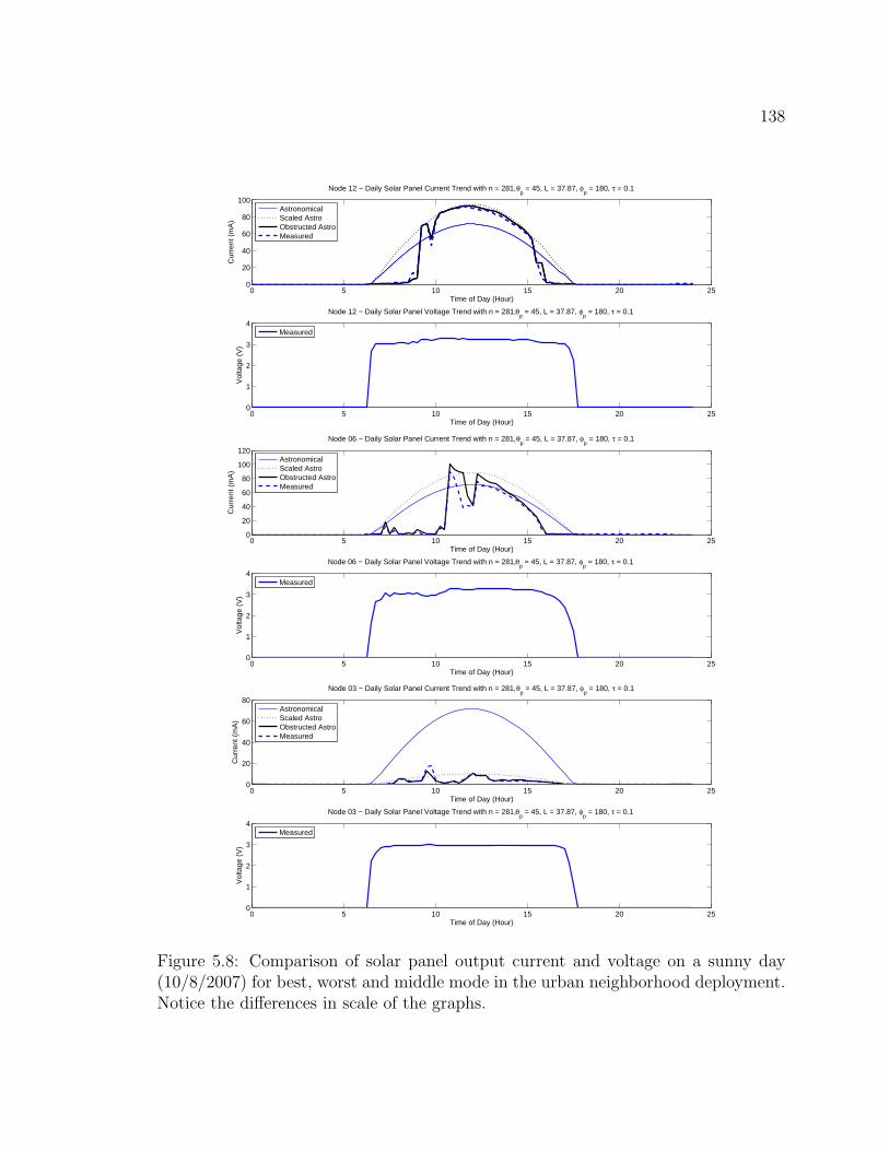
138

0 5 10 15 20 250

20

40

60

80

100

Time of Day (Hour)

Cur

rent

(m

A)

Node 12 − Daily Solar Panel Current Trend with n = 281, θp = 45, L = 37.87, φ

p = 180, τ = 0.1

0 5 10 15 20 250

1

2

3

4

Time of Day (Hour)

Vol

tage

(V

)

Node 12 − Daily Solar Panel Voltage Trend with n = 281, θp = 45, L = 37.87, φ

p = 180, τ = 0.1

AstronomicalScaled AstroObstructed AstroMeasured

Measured

0 5 10 15 20 250

20

40

60

80

100

120

Time of Day (Hour)

Cur

rent

(m

A)


p = 180, τ = 0.1


0 5 10 15 20 250

1

2

3

4

Time of Day (Hour)

Vol

tage

(V

)


p = 180, τ = 0.1

Measured

0 5 10 15 20 250

20

40

60

80

Time of Day (Hour)

Cur

rent

(m

A)


p = 180, τ = 0.1


0 5 10 15 20 250

1

2

3

4

Time of Day (Hour)

Vol

tage

(V

)


p = 180, τ = 0.1

Measured

Figure 5.8: Comparison of solar panel output current and voltage on a sunny day(10/8/2007) for best, worst and middle mode in the urban neighborhood deployment.Notice the differences in scale of the graphs.

139

0 5 10 15 20 250

20

40

60

80

100

120

Time of Day (Hour)

Cur

rent

(m

A)


p = 180, τ = 0.1


0 5 10 15 20 250

1

2

3

4

Time of Day (Hour)

Vol

tage

(V

)


p = 180, τ = 0.1

Measured

0 5 10 15 20 250

20

40

60

80

100

120

Time of Day (Hour)

Cur

rent

(m

A)


p = 180, τ = 0.1


0 5 10 15 20 250

1

2

3

4

Time of Day (Hour)

Vol

tage

(V

)


p = 180, τ = 0.1

Measured

0 5 10 15 20 250

20

40

60

80

Time of Day (Hour)

Cur

rent

(m

A)


p = 180, τ = 0.1


0 5 10 15 20 250

1

2

3

4

Time of Day (Hour)

Vol

tage

(V

)


p = 180, τ = 0.1

Measured

Figure 5.9: Comparison of solar panel output current and voltage on an overcast day(10/9/2007) for the urban neighborhood deployment.

140

Comparison with Estimation Models

Looking at the daily graph of solar current and voltage experienced at each of

the three representative nodes on a sunny day – shown in Figure 5.8 – we can see

the variations in available solar energy inputs among nodes throughout a day. Nodes

that generated very little solar energy still had a solar panel voltage above 3 volts for

the light portion of the day. This voltage is limited by the load – in this case, the

batteries. Thus, the solar voltage exhibits near binary behavior between 0 volts when

there is no incident light and its maximum voltage (as dictated by its load) any time

between dawn and dusk.

Additionally, these current graphs are plotted alongside the three estimation mod-

els (astronomical, scaled astronomical and obstructed astronomical) as a basis for

comparison. The measurement of the solar profile fits the astronomical model when

the solar panel has an unobstructed view of sunlight for a certain period of time. For

other cases, whether the solar panel is obstructed during part of the day (Node 12 and

Node 06) or the whole day (Node 03), the estimation from the astronomical model

deviates far from the measurement. The obstructed astronomical model captures the

shading effect and gives a better fitting to the measurement than the astronomical

model. On an overcast day, the gap between the measurement and the estimation

of each model becomes higher, because the estimation models capture time variation

and obstruction effects, but not the weather effects. Table 5.3 summarizes the solar

panel output measurement and estimations for both a sunny day (10/8/2007) and an

overcast day (10/9/2007). We can see that the astronomical model has higher esti-

mation error, as the node is obstructed for longer hours, thus the obstruction model

fits the measurement on any obstruction conditions.

We can also notice that the sporadic pattern of the solar energy received through-

out the day has implications for the daily power cycle introduced in Figure 3.7 as well;

the progression through the daily model may instead oscillate among the recharge,

saturation, and discharge phases during the daylight hours.

The urban neighborhood deployment demonstrated that even nodes with severe

arboreal and other occlusions received enough sunlight to sustain operation; that is,

1This effect is most pronounced in this figure (the solar energy doubles on a cloudy day for Node03), but appeared in other observations as well.

141

the nodes in the most shade still received at least 30 minutes of sunlight on both

sunny and cloudy days validating the prediction of our model and making us (falsely)

confident that our design would succeed in the forest watershed.

5.2.2 A Sensor Network in a Forest Watershed

Overall Trend

The blend of solar profiles seen by the nodes in the forest watershed was far less

diverse than the urban neighborhood as shown in Figure 5.10. Most of the nodes

received no more than 50 mWh of energy on any of the days of the deployment.

Just as in Figure 5.7, the lines represent nodes chosen to show the range of the solar

distribution. However, in Figure 5.10, the middle line represents the second-best

performing node (not the median), and the lowest line is for a node representative of

those that are receiving very limited energy. The stunning difference between the two

deployments is how much less solar energy was harvested in the forest watershed – the

best-performing node on a sunny day in the forest did not receive as much solar energy

as the median node on a cloudy day in the urban neighborhood. Additionally, Angelo

02 (and other sun-starved nodes like it) harvested less than the node consumption

each day. This daily energy deficit results in a negative number of surplus battery

days. It is important to note that these nodes are experiencing different degrees of

sun starvation – some are only consuming about half a day’s worth of battery energy

daily, while others are consuming a full day’s worth of energy daily. Still, a majority

of the nodes were not receiving sufficient solar energy to operate sustainably, causing

a finite lifetime for the network.

Comparison with Estimation Models

Figure 5.11, 5.12 and 5.13 show the trends of solar radiation and battery capacity

for the three representative nodes. In this forest deployment, most nodes are heav-

ily occluded and the astronomical model, which assumes unobstructed view of the

sky, does not effectively estimate the solar radiation, with estimation error 80.9% to

99.9%. The obstructed astronomical model fits the measurement within around 30%

of error for nodes with high radiation condition (Router 78) and medium radiation

142

10/14/07 10/21/07−100

0

100

200

300

400

500

600

700Daily Solar Energy Measurements at Angelo Reserve, CA (10/10/2007 to 10/25/2007)

Day

Dai

ly S

olar

Ene

rgy

Rec

eive

d (m

Whr

)

Router 78Router 77Angelo 02Mote Consumption

01/00/00 01/01/00−0.83

0

0.83

1.66

2.49

3.32

4.15

4.98

5.81

Effe

ctiv

e B

atte

ry D

ays

Figure 5.10: Scatter plot of solar energy received in the forest watershed deployment.Three representative nodes are highlighted.

143

10/14 10/21 10/28 11/04 11/110

500

1000

1500

2000

Date

Dai

ly S

olar

Pan

el E

nerg

y (m

Wh)

Router 78 − Solar Panel Output Trend from 10/11/07 to 11/09/07 , θp = 45, L = 37.87, φ

p = 180, τ = 0.1

AstronomicalScaled AstroObstructed AstroMeasurementLoad / Eff

sys

10/14 10/21 10/28 11/04 11/110

100

200

300

400

500

600

Date

Dai

ly S

olar

Pan

el E

nerg

y (m

Wh)

Router 78 − Solar Panel Output Trend (Enlarged) from 10/11/07 to 11/09/07 , θp = 45, L = 37.87, φ

p = 180, τ = 0.1


sys

10/14 10/21 10/28 11/04 11/112200

2250

2300

2350

2400

2450

2500

2550

Date

Dai

ly B

atte

ry C

apac

ity (

mA

h)

Router 78 − Battery Level Trend from 10/11/07 to 11/09/07 , θp = 45, L = 37.87, φ

p = 180, τ = 0.1

AstronomicalScaled AstroObstructed Astro

AstronomicalModel

Scaled AstroModel


Deviation from measurement 80.9% 75.4% 29.8%

Figure 5.11: Comparison of different radiation estimation methods for high radiationnode (Router 78) on forest deployment.

144

10/14 10/21 10/28 11/04 11/110

500

1000

1500

2000

Date

Dai

ly S

olar

Pan

el E

nerg

y (m

Wh)

Router 77 − Solar Panel Output Trend from 10/11/07 to 11/09/07 , θp = 45, L = 37.87, φ

p = 180, τ = 0.1


sys

10/14 10/21 10/28 11/04 11/110

20

40

60

80

100

Date

Dai

ly S

olar

Pan

el E

nerg

y (m

Wh)

Router 77 − Solar Panel Output Trend (Enlarged) from 10/11/07 to 11/09/07 , θp = 45, L = 37.87, φ

p = 180, τ = 0.1


sys

10/14 10/21 10/28 11/04 11/111600

1800

2000

2200

2400

Date

Dai

ly B

atte

ry C

apac

ity (

mA

h)

Router 77 − Battery Level Trend from 10/11/07 to 11/09/07 , θp = 45, L = 37.87, φ

p = 180, τ = 0.1


AstronomicalModel

Scaled AstroModel



Figure 5.12: Comparison of different radiation estimation methods for medium radi-ation node (Router 77) on forest deployment.

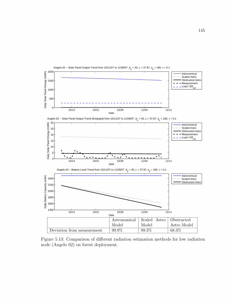
145

10/14 10/21 10/28 11/04 11/110

500

1000

1500

2000

Date

Dai

ly S

olar

Pan

el E

nerg

y (m

Wh)

Angelo 02 − Solar Panel Output Trend from 10/11/07 to 11/09/07 , θp = 45, L = 37.87, φ

p = 180, τ = 0.1


sys

10/14 10/21 10/28 11/04 11/110

5

10

15

20

25

30

Date

Dai

ly S

olar

Pan

el E

nerg

y (m

Wh)

Angelo 02 − Solar Panel Output Trend (Enlarged) from 10/11/07 to 11/09/07 , θp = 45, L = 37.87, φ

p = 180, τ = 0.1


sys

10/14 10/21 10/28 11/04 11/111400

1600

1800

2000

2200

2400

Date

Dai

ly B

atte

ry C

apac

ity (

mA

h)

Angelo 02 − Battery Level Trend from 10/11/07 to 11/09/07 , θp = 45, L = 37.87, φ

p = 180, τ = 0.1


AstronomicalModel

Scaled AstroModel



Figure 5.13: Comparison of different radiation estimation methods for low radiationnode (Angelo 02) on forest deployment.

146

condition (Router 77). This 30% difference is due to the non-stationary changes such

as a weather effect. For low radiation node (Angelo 02), the effect of non-stationary

changes becomes more important with the estimation error 68%.

Lessons from Forest Deployment

Figures 5.14 and 5.15 show the solar current and voltage of the three representative

nodes on a sunny and overcast day, respectively. The solar voltages exhibit the

familiar binary behavior in both cases. The solar currents noticeably suffer on the

overcast day, but the heavily shaded node slightly improves its energy harvesting.

Perhaps the most important observation is how spiky the solar profile is for the nodes

that receive reasonable amounts of solar energy.

It appears that the primary limitation of available solar energy in the forest context

is not the amount of light, but the speckled nature of the light that is present. Rarely

is the spot of light that falls on even our small panels large enough to illuminate the

entire panel. Overcast days diffuse the shadows, reducing the spotting. An individual

solar cell produces about 0.5 volts, so several are placed in series within the panel

to provide a useful output voltage. For example, our panels have two chains of eight

cells in series (Figure 5.16(a)). The current of the cell is determined by its area, and

cells can be interconnected in various serial-parallel networks. The problem is that

when a single cell in a serial chain is not well-illuminated, it limits the current flow

through the entire chain.

In order to see the effect of shading in a solar panel that consists of an array of

solar cells in series or parallel, we built a solar panel array with four solar panels in

three different configurations: (i) four panels in parallel, (ii) two parallel chains of

two panels in series, (iii) four panels in series. For each configuration, we measured

the short circuit current of the solar panel array. We also measured the short circuit

current when we covered one of the panels to emulate shading (Figure 5.16(b), 5.16(c)

and 5.16(d)). Figure 5.17 shows the result for the experiment. When all panels are

connected in parallel, the decrease in short circuit current of the solar panel array is

directly proportional to the covered panels (first figure). When panels are connected

in two parallel chains of two panels in series, covering one panel caused one of the

two chains to shutdown. This is the case for the 4.0V-100mA polycrystalline silicon

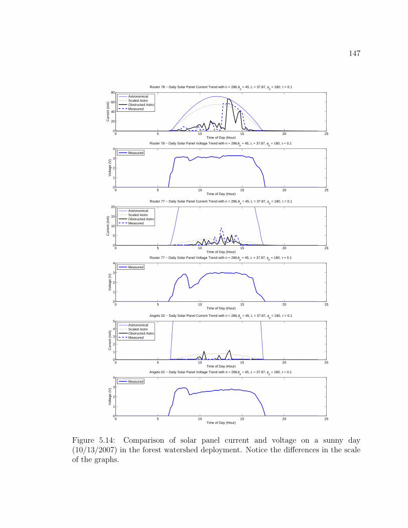
147

0 5 10 15 20 250

20

40

60

80

Time of Day (Hour)

Cur

rent

(m

A)

Router 78 − Daily Solar Panel Current Trend with n = 286, θp = 45, L = 37.87, φ

p = 180, τ = 0.1


0 5 10 15 20 250

1

2

3

4

Time of Day (Hour)

Vol

tage

(V

)

Router 78 − Daily Solar Panel Voltage Trend with n = 286, θp = 45, L = 37.87, φ

p = 180, τ = 0.1

Measured

0 5 10 15 20 250

5

10

15

20

Time of Day (Hour)

Cur

rent

(m

A)


p = 180, τ = 0.1


0 5 10 15 20 250

1

2

3

4

Time of Day (Hour)

Vol

tage

(V

)


p = 180, τ = 0.1

Measured

0 5 10 15 20 250

1

2

3

4

5

Time of Day (Hour)

Cur

rent

(m

A)

Angelo 02 − Daily Solar Panel Current Trend with n = 286, θp = 45, L = 37.87, φ

p = 180, τ = 0.1


0 5 10 15 20 250

1

2

3

4

Time of Day (Hour)

Vol

tage

(V

)

Angelo 02 − Daily Solar Panel Voltage Trend with n = 286, θp = 45, L = 37.87, φ

p = 180, τ = 0.1

Measured

Figure 5.14: Comparison of solar panel current and voltage on a sunny day(10/13/2007) in the forest watershed deployment. Notice the differences in the scaleof the graphs.

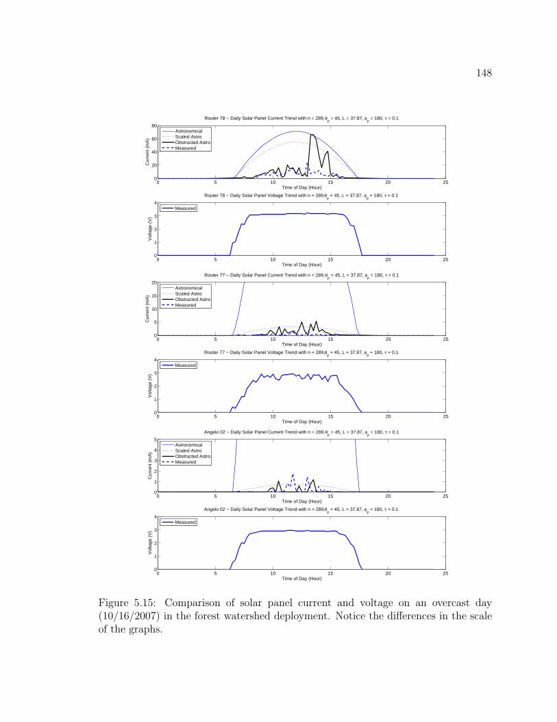
148

0 5 10 15 20 250

20

40

60

80

Time of Day (Hour)

Cur

rent

(m

A)


p = 180, τ = 0.1


0 5 10 15 20 250

1

2

3

4

Time of Day (Hour)

Vol

tage

(V

)


p = 180, τ = 0.1

Measured

0 5 10 15 20 250

5

10

15

20

Time of Day (Hour)

Cur

rent

(m

A)


p = 180, τ = 0.1


0 5 10 15 20 250

1

2

3

4

Time of Day (Hour)

Vol

tage

(V

)


p = 180, τ = 0.1

Measured

0 5 10 15 20 250

1

2

3

4

5

Time of Day (Hour)

Cur

rent

(m

A)

Angelo 02 − Daily Solar Panel Current Trend with n = 289, θp = 45, L = 37.87, φ

p = 180, τ = 0.1


0 5 10 15 20 250

1

2

3

4

Time of Day (Hour)

Vol

tage

(V

)

Angelo 02 − Daily Solar Panel Voltage Trend with n = 289, θp = 45, L = 37.87, φ

p = 180, τ = 0.1

Measured

Figure 5.15: Comparison of solar panel current and voltage on an overcast day(10/16/2007) in the forest watershed deployment. Notice the differences in the scaleof the graphs.

149

8 series cells8 series cells

2 parallel cell arrays

(a) Cell configuration of 4V-100mA polycrystalline silicon so-

lar panel

A

(b) 4 parallel panels with one

panel covered

A

(c) 2-parallel and 2-series pan-

els with one panel covered

A

(d) 4 parallel panels with one

panel covered

Figure 5.16: Different configurations of solar panel array

panel we used (second figure). When panels are connected in series, covering one

panel caused the whole array to shutdown (third figure).

Thus, enlarging the panel does not necessarily increase the power output in speck-

led light. Instead, many small panels should be connected in a highly parallel con-

figuration. Large residential and commercial arrays have this characteristic because

of the sheer number of panels involved. One possibility of a highly parallel configu-

ration in micro-solar power systems is to use a flexible solar panel (Figure 5.18(a)).

Since each cell of a flexible solar panel is connected in parallel, covering x-percent of

the whole cells causes only x-percent drop in the solar panel current (Figure 5.18(b)

and 5.18(c)). We find this has the same trend as the parallel solar panel configura-

tion (Figure 5.16). One drawback of using a flexible solar panel is its lower material

efficiency, which implies that we need a larger area of flexible solar panel than the

polycrystalline silicon panel to output the equivalent amount of current under unob-

structed radiation condition. However, resilience to the shading effect compensates

the cost of lower material efficiency in a forest environment.

150

0 10

100

200

300

400

500

Number ofcovered panels

Sho

rt−

circ

uit c

urre

nt o

f sol

ar p

anel

arr

ay (

mA

) 4 parallel4V−100mA panels

0 10

100

200

300

400

500


Sho

rt−

circ

uit c

urre

nt o

f sol

ar p

anel

arr

ay (

mA

) 2 parallel and 2 series4V−100mA panels

0 10

100

200

300

400

500


Sho

rt−

circ

uit c

urre

nt o

f sol

ar p

anel

arr

ay (

mA

) 4 series4V−100mA panels

Figure 5.17: Effect of shading on polycrystalline silicon solar panel

Increasing the battery size also has surprising implications. With the low daily

consumption of a well-engineered environmental monitoring application, it is reason-

able to size batteries to last for several seasons. In deciduous forests, this would allow

nodes to store up all their energy after the leaves fall. Even in coniferous forests, it

means that energy can be collected when the interaction of the canopy and the sun an-

gle are most favorable. Additional improvements are possible through utilizing more

efficient regulators with somewhat more complex circuit requirements. Exploration

of novel collectors and storage profiles for important solar-challenged environments

will drive further improvements in the models as well as the physical design.

5.3 Summary

In this chapter, we have developed a reference platform, the HydroWatch node, to

validate the simulation model of micro-solar power systems. It is designed to operate

perpetually even on half an hour of sunlight per day while sensing the environment

and networking over multiple hops in low-power mode. From the evaluation of over

twenty HydroWatch nodes that were deployed in an urban neighborhood and forest

watershed environment, we were able to observe the following. First, the obstructed-

astronomical model estimated solar radiation with modest error while each sensor

node was under various obstruction and weather conditions. Second, all the sensor

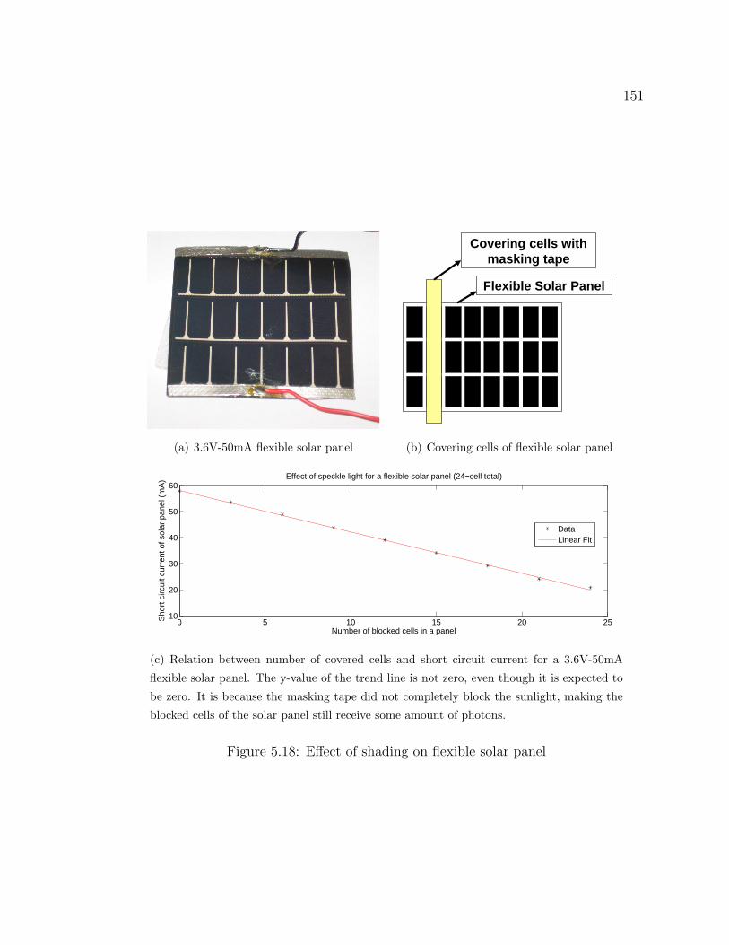
151

(a) 3.6V-50mA flexible solar panel

Covering cells withmasking tape

Flexible Solar Panel

(b) Covering cells of flexible solar panel

0 5 10 15 20 2510

20

30

40

50

60

Number of blocked cells in a panel

Sho

rt c

ircui

t cur

rent

of s

olar

pan

el (

mA

) Effect of speckle light for a flexible solar panel (24−cell total)

DataLinear Fit

(c) Relation between number of covered cells and short circuit current for a 3.6V-50mA

flexible solar panel. The y-value of the trend line is not zero, even though it is expected to

be zero. It is because the masking tape did not completely block the sunlight, making the

blocked cells of the solar panel still receive some amount of photons.

Figure 5.18: Effect of shading on flexible solar panel

152

nodes in the urban neighborhood deployment accumulated sufficient solar energy

for perpetual operation, validating the capacity planning for the HydroWatch node.

Third, most nodes in the forest deployment did not collect sufficient solar energy,

showing that a different solar panel should be used depending on radiation conditions:

a flexible solar panel is more suitable for the forest environment though it has a lower

efficiency than a polycrystalline silicon panel; its cells are connected in parallel and

this allows the flexible panel to produce electricity even when part of the panel is

shadowed.

153

Chapter 6

Predicting the Long-term Behavior

of a Micro-Solar Power System

In Chapter 4, we introduced an obstructed astronomical model that estimates

solar radiation under obstructions. This model fits into the measurements well on

a sunny day (Figure 6.1 (a)), but does not on an overcast day. The solar radiation

becomes smaller due to the weather effect and the obstructed model does not catch

this variation well with the estimation error getting higher (Figure 6.1 (b)).

In this chapter, we first study the effect of weather variations on solar radiation

(Section 6.1). We use a long-term measurement of HydroWatch weather nodes that

is taken in an obstructed environment, and compare the measurement data with

the estimation models. Then, we develop a possible model for the solar radiation

under weather variations using commercially available weather data (Section 6.2).

We evaluate its validity by comparing the solar radiation estimate with the long-term

measurement data of the HydroWatch weather nodes (Section 6.3).

6.1 Accounting for the Weather Effect

6.1.1 Experimental Set-up

In order to see the effect of weather variations, we deployed five HydroWatch

weather nodes on the rooftop of the Valley Life Science Building (VLSB) in UC

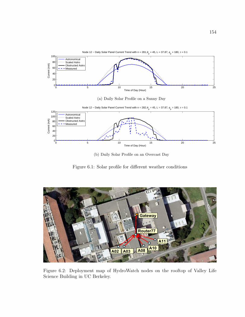
154

0 5 10 15 20 250

20

40

60

80

100

Time of Day (Hour)

Cur

rent

(m

A)


p = 180, τ = 0.1

0 5 10 15 20 250

1

2

3

4

Time of Day (Hour)

Vol

tage

(V

)


p = 180, τ = 0.1


Measured(a) Daily Solar Profile on a Sunny Day

0 5 10 15 20 250

20

40

60

80

100

120

Time of Day (Hour)

Cur

rent

(m

A)


p = 180, τ = 0.1


0 5 10 15 20 250

1

2

3

4

Time of Day (Hour)

Vol

tage

(V

)


p = 180, τ = 0.1

Measured(b) Daily Solar Profile on an Overcast Day

Figure 6.1: Solar profile for different weather conditions

Gateway

A02 A03 A08 A10A11

Router77

Figure 6.2: Deployment map of HydroWatch nodes on the rooftop of Valley LifeScience Building in UC Berkeley.

155

Berkeley where micro-solar nodes can get solar radiation without any obstructions

from trees or other buildings (Figure 6.2). Since there are no obstructions between

each node and the sun, the measurement of the solar panel output depends only on

the diurnal and seasonal variation of solar radiation and the weather variation. The

astronomical model, which is explained in Chapter 4, gives an estimation of diur-

nal and seasonal variation of the solar radiation. We use the obstructed astronomical

model in order to fit the astronomical model to the measurement, then we account for

the weather effect by comparing the solar panel output measurement with the predic-

tion from the obstructed astronomical model. For this experiment, five HydroWatch

weather nodes were deployed, and the following parameters are used for the external

environment:

• Day of the Year (n) : The experiment was conducted from 12/22/2007 (n =

356) to 4/15/2008 (n = 365 + 106).

• Latitude (L) : The experiment was done in Berkeley, CA, which is at 37.87◦N.

• Solar Panel Inclination (θp) and Orientation (φp) : Depending on the

solar panel inclination, the five HydroWatch weather nodes were sorted into

two groups. Nodes A02 and A08 had their panels tilted 45◦ (θp = 45) facing

south (φp = 180). And nodes A03, A10 and A11 had their panels flat to the

ground (θp = 0).

6.1.2 Results

Figure 6.3 compares the daily solar panel energy measurement with a few estima-

tion models. From this plot, we can observe the following:

• Seasonal Variation: The three estimation models (astronomical, scaled astro-

nomical and obstructed astronomical) capture the seasonal variation well and

the obstructed astronomical model tracks the peak of the measurement.

• Weather Effect: The obstructed astronomical model deviates from the mea-

surement within about 30% due to weather.

156

01/01 02/01 03/01 04/010

500

1000

1500

2000

2500

3000

Date

Sol

ar P

anel

Ene

rgy

(mW

h)A02 − Solar Panel Output Trend from 12/22/07 to 04/15/08 , θ

p = 45, L = 37.87, φ

p = 180, τ = 0.1


sys

01/01 02/01 03/01 04/012350

2400

2450

2500

2550

Date

Bat

tery

Cap

acity

(m

Ah)

A02 − Battery Level Trend from 12/22/07 to 04/15/08 , θp = 45, L = 37.87, φ

p = 180, τ = 0.1


01/01 02/01 03/01 04/010

0.2

0.4

0.6

0.8

1

Date

Dev

iatio

n (0

− 1

)

A02 − Deviation of Solar Panel Output Measurement from Estimation (12/22/07 to 04/15/08)

Obstructed Astro

01/01 02/01 03/01 04/010

500

1000

1500

2000

2500

3000

Date

Sol

ar P

anel

Ene

rgy

(mW

h)

A03 − Solar Panel Output Trend from 12/22/07 to 04/15/08 , θp = 0, L = 37.87, φ

p = 180, τ = 0.1


sys

01/01 02/01 03/01 04/012200

2250

2300

2350

2400

2450

2500

2550

Date

Bat

tery

Cap

acity

(m

Ah)


p = 180, τ = 0.1


01/01 02/01 03/01 04/010

0.2

0.4

0.6

0.8

1

Date

Dev

iatio

n (0

− 1

)


Obstructed Astro

01/01 02/01 03/01 04/010

500

1000

1500

2000

2500

Date

Sol

ar P

anel

Ene

rgy

(mW

h)


p = 180, τ = 0.1


sys

01/01 02/01 03/01 04/012350

2400

2450

2500

2550

Date

Bat

tery

Cap

acity

(m

Ah)


p = 180, τ = 0.1


01/01 02/01 03/01 04/010

0.2

0.4

0.6

0.8

1

Date

Dev

iatio

n (0

− 1

)


Obstructed Astro

01/01 02/01 03/01 04/010

500

1000

1500

2000

2500

3000

Date

Sol

ar P

anel

Ene

rgy

(mW

h)


p = 180, τ = 0.1


sys

01/01 02/01 03/01 04/012200

2250

2300

2350

2400

2450

2500

2550

Date

Bat

tery

Cap

acity

(m

Ah)


p = 180, τ = 0.1


01/01 02/01 03/01 04/010

0.2

0.4

0.6

0.8

1

Date

Dev

iatio

n (0

− 1

)


Obstructed Astro

01/01 02/01 03/01 04/010

500

1000

1500

2000

2500

3000

Date

Sol

ar P

anel

Ene

rgy

(mW

h)


p = 180, τ = 0.1


sys

01/01 02/01 03/01 04/012200

2250

2300

2350

2400

2450

2500

2550

Date

Bat

tery

Cap

acity

(m

Ah)


p = 180, τ = 0.1


01/01 02/01 03/01 04/010

0.2

0.4

0.6

0.8

1

Date

Dev

iatio

n (0

− 1

)


Obstructed Astro

Figure 6.3: Seasonal solar radiation variation of HydroWatch weather nodes on therooftop of Valley Life Science building in UC Berkeley

157

01/01 02/01 03/01 04/010

500

1000

1500

2000

2500

3000

Date

Sol

ar P

anel

Ene

rgy

(mW

h)


p = 180, τ = 0.1


sys

01/01 02/01 03/01 04/012350

2400

2450

2500

2550

Date

Bat

tery

Cap

acity

(m

Ah)


p = 180, τ = 0.1


01/01 02/01 03/01 04/010

0.2

0.4

0.6

0.8

1

Date

Dev

iatio

n (0

− 1

)A02 − Deviation of Solar Panel Output Measurement from Estimation (12/22/07 to 04/15/08)

Obstructed Astro

01/01 02/01 03/01 04/010

500

1000

1500

2000

2500

3000

Date

Sol

ar P

anel

Ene

rgy

(mW

h)


p = 180, τ = 0.1


sys

01/01 02/01 03/01 04/012200

2250

2300

2350

2400

2450

2500

2550

Date

Bat

tery

Cap

acity

(m

Ah)


p = 180, τ = 0.1


01/01 02/01 03/01 04/010

0.2

0.4

0.6

0.8

1

Date

Dev

iatio

n (0

− 1

)


Obstructed Astro

01/01 02/01 03/01 04/010

500

1000

1500

2000

2500

Date

Sol

ar P

anel

Ene

rgy

(mW

h)


p = 180, τ = 0.1


sys

01/01 02/01 03/01 04/012350

2400

2450

2500

2550

Date

Bat

tery

Cap

acity

(m

Ah)


p = 180, τ = 0.1


01/01 02/01 03/01 04/010

0.2

0.4

0.6

0.8

1

Date

Dev

iatio

n (0

− 1

)


Obstructed Astro

01/01 02/01 03/01 04/010

500

1000

1500

2000

2500

3000

Date

Sol

ar P

anel

Ene

rgy

(mW

h)


p = 180, τ = 0.1


sys

01/01 02/01 03/01 04/012200

2250

2300

2350

2400

2450

2500

2550

Date

Bat

tery

Cap

acity

(m

Ah)


p = 180, τ = 0.1


01/01 02/01 03/01 04/010

0.2

0.4

0.6

0.8

1

Date

Dev

iatio

n (0

− 1

)


Obstructed Astro

01/01 02/01 03/01 04/010

500

1000

1500

2000

2500

3000

Date

Sol

ar P

anel

Ene

rgy

(mW

h)


p = 180, τ = 0.1


sys

01/01 02/01 03/01 04/012200

2250

2300

2350

2400

2450

2500

2550

Date

Bat

tery

Cap

acity

(m

Ah)


p = 180, τ = 0.1


01/01 02/01 03/01 04/010

0.2

0.4

0.6

0.8

1

Date

Dev

iatio

n (0

− 1

)


Obstructed Astro

Figure 6.4: Deviation of the solar energy measurement from the estimate for theHydroWatch weather nodes deployment on the rooftop of Valley Life Science buildingin UC Berkeley

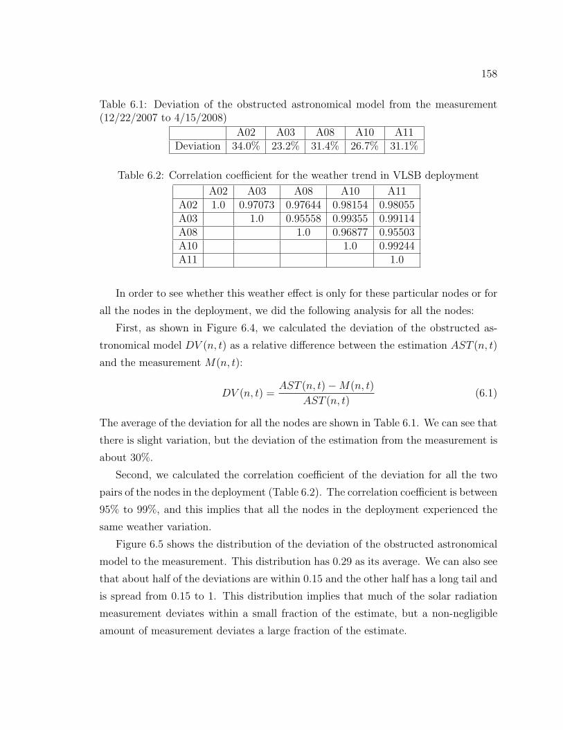
158

Table 6.1: Deviation of the obstructed astronomical model from the measurement(12/22/2007 to 4/15/2008)

A02 A03 A08 A10 A11Deviation 34.0% 23.2% 31.4% 26.7% 31.1%

Table 6.2: Correlation coefficient for the weather trend in VLSB deployment

A02 A03 A08 A10 A11A02 1.0 0.97073 0.97644 0.98154 0.98055A03 1.0 0.95558 0.99355 0.99114A08 1.0 0.96877 0.95503A10 1.0 0.99244A11 1.0

In order to see whether this weather effect is only for these particular nodes or for

all the nodes in the deployment, we did the following analysis for all the nodes:

First, as shown in Figure 6.4, we calculated the deviation of the obstructed as-

tronomical model DV (n, t) as a relative difference between the estimation AST (n, t)

and the measurement M(n, t):

DV (n, t) =AST (n, t)−M(n, t)

AST (n, t)(6.1)

The average of the deviation for all the nodes are shown in Table 6.1. We can see that

there is slight variation, but the deviation of the estimation from the measurement is

about 30%.

Second, we calculated the correlation coefficient of the deviation for all the two

pairs of the nodes in the deployment (Table 6.2). The correlation coefficient is between

95% to 99%, and this implies that all the nodes in the deployment experienced the

same weather variation.

Figure 6.5 shows the distribution of the deviation of the obstructed astronomical

model to the measurement. This distribution has 0.29 as its average. We can also see

that about half of the deviations are within 0.15 and the other half has a long tail and

is spread from 0.15 to 1. This distribution implies that much of the solar radiation

measurement deviates within a small fraction of the estimate, but a non-negligible

amount of measurement deviates a large fraction of the estimate.

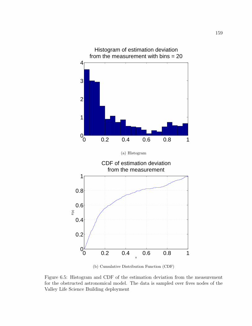
159

0 0.2 0.4 0.6 0.8 10

1

2

3

4

Histogram of estimation deviationfrom the measurement with bins = 20

(a) Histogram

0 0.2 0.4 0.6 0.8 10

0.2

0.4

0.6

0.8

1

x

F(x

)

CDF of estimation deviationfrom the measurement

(b) Cumulative Distribution Function (CDF)

Figure 6.5: Histogram and CDF of the estimation deviation from the measurementfor the obstructed astronomical model. The data is sampled over fives nodes of theValley Life Science Building deployment

160

6.2 Developing Weather Effect Model

In the previous section, we have shown that solar radiation estimation using as-

tronomical and obstruction models has a variation of about 30% from the actual

measurement due to weather effects. A natural question to ask is whether it is pos-

sible to predict solar radiation under weather variations. In order to answer this

question, we develop a weather effect model using publicly available data and eval-

uate whether the model can predict the variation of solar radiation with sufficient

accuracy. Among the various kinds of data measured in weather stations, there are

several metrics related to the transfer rate of solar radiation under weather effects:

atmospheric turbidity, horizontal visibility, and cloud cover. In this section, we model

solar radiation under weather effects using these metrics and validate each model

against extensive data from publicly available weather stations.

6.2.1 Atmospheric Turbidity

Atmospheric turbidity, or simply turbidity is used as a measure of air pollution

in the atmospheric science community and is known to be highly correlated with

solar radiation [PFR78, RV82, CH88]. As sunlight traverses the atmosphere, solar

irradiance is degraded by several causes: sunlight can be scattered by air molecules

(Rayleigh scattering); it can be absorbed by atmospheric gases such as ozone, water

vapor and carbon dioxide; or it can be absorbed by aerosols such as clouds, fog and

smog. Turbidity accounts for the degradation of solar radiation due to aerosols, and

it is defined as the ratio of solar irradiance degraded by aerosols and extraterrestrial

solar irradiance, which can be estimated using an astronomical model of solar radia-

tion. Since solar irradiance and Rayleigh scattering varies depending on wavelength

of sunlight, turbidity is typically defined at a particular wavelength. Turbidity at

wavelength λ, B(λ), is a non-negative number and is logarithmically related to the

ratio of actual solar irradiance J(λ) and extraterrestrial solar irradiance J0(λ) [RV82]:

J(λ)/J0(λ) = 10−(R(λ)+Z(λ)+B(λ))m (6.2)

where R is the Rayleigh scattering coefficient, Z is the gaseous absorption coeffi-

cient, and m is the optical air mass, which is the relative length of sunlight through

161

0 2000 4000 6000 8000 100000

2000

4000

6000

8000

10000

12000

Daily radiation measurement (Wh/m2)

Dai

ly r

adia

tion

estim

atio

n (W

h/m

2 )

Correlation with turbidity : 0.84656 (Golden, CO − 2008)

0 1 2 3 4 5 6 7

x 104

0

1

2

3

4

5

6

7x 10

4

7−day radiation measurement (Wh/m2)

7−da

y ra

diat

ion

estim

atio

n (W

h/m

2 )


0 2 4 6 8 10 12 14

x 104

0

2

4

6

8

10

12x 10

4

15−day radiation measurement (Wh/m2)

15−

day

radi

atio

n es

timat

ion

(Wh/

m2 )


0 0.5 1 1.5 2 2.5

x 105

0

0.5

1

1.5

2

2.5x 10

5

30−day radiation measurement (Wh/m2)30

−da

y ra

diat

ion

estim

atio

n (W

h/m

2 )

Correlation with turbidity : 0.96588 (Golden, CO − 2008)Figure 6.6: Correlation of daily solar radiation estimation using turbidity and actualmeasurements at Golden, CO from 1/1/2008 to 12/31/2008

the atmosphere compared to when sunlight is normal to the Earth’s surface. While

turbidity is defined at a particular wavelength, we consider modeling solar radiation

under weather variation using turbidity at 500nm, which has the highest intensity

across the solar radiation spectrum. Suppose turbidity and the solar radiation esti-

mate from the astronomical model are given as B(n, t) and AST (n, t) on day n and

time t, we can estimate the daily solar radiation under the influence of turbidity,

RB(n, t) using the logarithmic relation of solar radiation and turbidity:

RB(n) =

∫ 24h

0h

RB(n, t)dt (6.3)

=

∫ 24h

0h

k · AST (n, t) · e−B(n,t)dt

where k is a constant.

In order to validate this turbidity-to-radiation model, we compare the correla-

tion coefficient between the solar radiation under the influence of turbidity and the

solar radiation measurement using a publicly availble database provided by the Mea-

surement and Instrumentation Data Center (MIDC) [BMS]. The MIDC database

provides data for solar radiation measurement, turbidity and astronomical estima-

tion of solar radiation at a per-minute or per-hour scale. From this raw data, we can

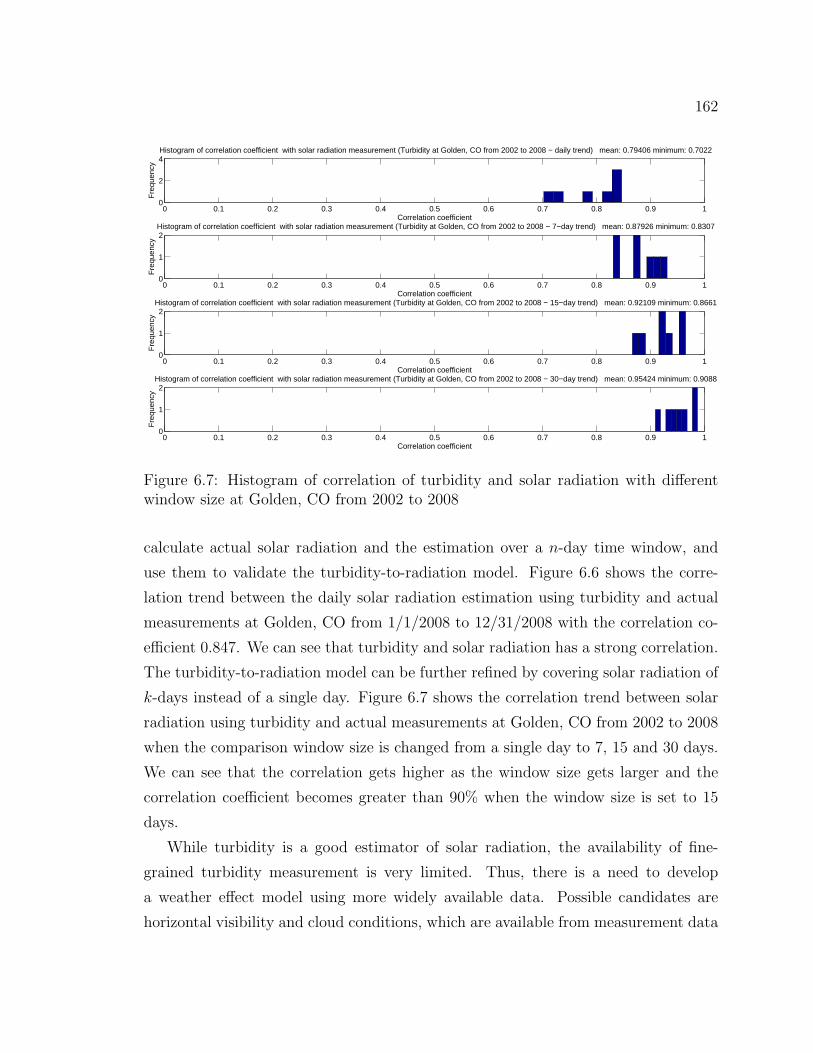
162

0 0.1 0.2 0.3 0.4 0.5 0.6 0.7 0.8 0.9 10

2

4

Correlation coefficient

Fre

quen

cyHistogram of correlation coefficient with solar radiation measurement (Turbidity at Golden, CO from 2002 to 2008 − daily trend) mean: 0.79406 minimum: 0.7022

0 0.1 0.2 0.3 0.4 0.5 0.6 0.7 0.8 0.9 10

1

2


Fre

quen

cy

Histogram of correlation coefficient with solar radiation measurement (Turbidity at Golden, CO from 2002 to 2008 − 7−day trend) mean: 0.87926 minimum: 0.8307

0 0.1 0.2 0.3 0.4 0.5 0.6 0.7 0.8 0.9 10

1

2


Fre

quen

cy


0 0.1 0.2 0.3 0.4 0.5 0.6 0.7 0.8 0.9 10

1

2


Fre

quen

cy


Figure 6.7: Histogram of correlation of turbidity and solar radiation with differentwindow size at Golden, CO from 2002 to 2008

calculate actual solar radiation and the estimation over a n-day time window, and

use them to validate the turbidity-to-radiation model. Figure 6.6 shows the corre-

lation trend between the daily solar radiation estimation using turbidity and actual

measurements at Golden, CO from 1/1/2008 to 12/31/2008 with the correlation co-

efficient 0.847. We can see that turbidity and solar radiation has a strong correlation.

The turbidity-to-radiation model can be further refined by covering solar radiation of

k-days instead of a single day. Figure 6.7 shows the correlation trend between solar

radiation using turbidity and actual measurements at Golden, CO from 2002 to 2008

when the comparison window size is changed from a single day to 7, 15 and 30 days.

We can see that the correlation gets higher as the window size gets larger and the

correlation coefficient becomes greater than 90% when the window size is set to 15

days.

While turbidity is a good estimator of solar radiation, the availability of fine-

grained turbidity measurement is very limited. Thus, there is a need to develop

a weather effect model using more widely available data. Possible candidates are

horizontal visibility and cloud conditions, which are available from measurement data

163

at most airports and other weather stations.

6.2.2 Horizontal Visibility and Cloud Condition

Horizontal visibility, which is monitored at most airports to ensure air traffic

safety, is the distance one can see horizontally with a maximum of 10.0 miles or 16.1

km. With horizontal visibility and a solar radiation estimate from the astronomi-

cal model being given, we can estimate daily solar radiation under the influence of

the visibility using the observations of Peterson et al. on the relationship between

horizontal visibility and the ultra-violet (UV) spectrum of solar irradiance [PFR78]:

Peterson et al. stated that visibility and UV irradiance had a strong correlation below

10km of visibility while UV irradiance was only slightly correlated with visibility of

12km or above. While their observation was about visibility and UV irradiance, we

apply it to develop a weather effect model that will estimate solar radiation (not just

UV spectrum) from horizontal visibility.

When the horizontal visibility and solar radiation estimate from the astronomical

model are given as V (n, t) and AST (n, t) on day n and time t, we can estimate the

daily solar radiation under the influence of visibility RV (n) as follows:

RV (n) =

∫ 24h

0h

V (n, t)

Vknee· AST (n, t)dt (6.4)

V (n, t) =

Vknee V (n, t) ≥ Vknee

V (n, t) otherwise(6.5)

where we set Vknee as 12.0 km.

Cloud condition is the percentage of the sky covered by clouds, and it is used to

determine the cloudiness of the sky at a particular location. Depending on whether

we count all visible clouds or only opaque clouds, cloud condition can be further

divided into total cloud cover and opaque cloud cover. For a given cloud condition

W (n, t) and solar radiation estimate from the astronomical model AST (n, t) on day

n and time t, we can estimate RW (n), the daily solar radiation under the influence

of cloud condition on day n, as follows:

RW (n) =

∫ 24h

0h

W (n, t) · AST (n, t)dt (6.6)

164

Table 6.3: Measurement sites used from the National Solar Radiation Data BaseLocation

Denver Centennial Airport, CO Broomfield / Jeffco Airport, COTallahassee Regional Airport, FL Boise Air Terminal, ORJoslin Field Magic Valley Airport, ID Univ. of Illinois Willard Airport, ILWolf Point International Airport, MT Mercury Desert Rock Airport, NVAlbuquerque International Airport, NM Elizabeth City Coast Guard Airport, NCBismarck Municipal Airport, ND Ponca City Municipal Airport, OKBurns Municipal Airport, OR Eugene Mahlon Sweet Airport, ORKlamath Falls Intl Airport, OR Medford Rogue Valley International Airport, ORState College Airport, PA Abilene Regional Airport, TXAmarillo International Airport, TX Austin Mueller Municipal Airport, TXCorpus Christi Intl Airport, TX Del Rio Airport, TXEl Paso International Airport, TX Houston Ellington Air Force Base, TXLaredo International Airport, TX Longview Gregg County Airport, TXMcAllen Miller International Airport, TX Washington DC Dulles International Airport, VASalt Lake City International Airport, UT Moab / Canyonlands Airport, UTSeattle Boeing Field, WA Spokane International Airport, WABluefieldMercer Co, WV Madison Dane Co Regional Airport, WIRock Springs Airport, WY

In order to validate weather effect models with horizontal visibility and cloud con-

dition, we compare the solar radiation estimate using weather effect models and the

actual solar radiation measurements from 35 sites during 1991 to 2005 using historical

measurements from the National Solar Radiation Data Base [NSR]. Table 6.3 lists

the sites whose measurement data are used in our study.

Figure 6.8 and 6.9 show the correlation of solar radiation measurement and esti-

mate when we use visibility, total cloud cover and opaque cloud cover with the sliding

window size as 1, 7, 15 and 30 days. For the weather effect models using horizontal

visibility, total cloud cover and opaque cloud cover, we can observe the following:

First, the weather effect models show high correlation with the actual measure-

ments when the estimation is based on a sufficient number of samples. For example,

weather effect models with total cloud cover, opaque cloud cover and horizontal visi-

bility have mean correlation of 89%, 93% and 96% for a window size of 15 days.

Second, the estimation quality of the weather effect models improves as we increase

the window size, but it reaches a sweet spot at 15 days. When we increased the

window size from 15 days to 30 days, the improvement in the correlation coefficient

was marginal.

Third, horizontal visibility is a better predictor of solar radiation than total cloud

cover or opaque cloud cover. The mean and the minimum of the correlation coefficient

of horizontal visibility is 96% and 79% with a 15-day window. Whereas, total cloud

165

cover and opaque cloud cover have a much wider distribution. While the mean of their

correlation coefficients are about 90%, the minimum of the correlation coefficients are

much smaller, making long tails (9% and 10%).

6.3 Evaluating Weather Effect Model

In the previous section, we have shown that horizontal visibility and cloud condi-

tion can be used to estimate the solar radiation under the weather effect because they

have a high correlation with solar radiation when being averaged over multiple days.

Also the data is widely available from many weather stations. In this section, we

validate this idea with a concrete example. We will develop a solar radiation weather

effect model using the historical data of horizontal visibility and cloud conditions

from a publicly available weather station and compare it with the 5-month long solar

radiation measurements from our reference implementation of a micro-solar power

system.

6.3.1 Defining Solar Radiation Estimators

In order to develop a weather effect component, we use data from a publicly

available online weather station, Wunderground [Wun]. Wunderground provides a

live and archived view of several weather metrics for a number of weather stations

across the United States. We have used archived data of horizontal visibility and

cloud conditions for the Oakland International Airport, which is the nearest weather

station to the measurement site at UC Berkeley, that provides fine-grained data of

horizontal visibility and cloud conditions.

Suppose the solar radiation estimation without weather effect is given as AST (t)

and the weather factor W (t) can be represented as a number between 0 and 1. Then,

the solar radiation with weather effect RW (t) can be represented as a product of

AST (t) and W (t)

RW (t) = W (t) · AST (t) (6.7)

Figure 6.10 shows a snapshot of an hourly weather data report from Wunderground

which includes horizontal visibility and cloud conditions. Horizontal visibility is re-

166

0 0.1 0.2 0.3 0.4 0.5 0.6 0.7 0.8 0.9 10

50

100

150


Fre

quen

cyHistogram of correlation coefficient with solar radiation measurement (Total cloud cover − daily trend) mean: 0.81553 minimum: 0.0316

0 0.1 0.2 0.3 0.4 0.5 0.6 0.7 0.8 0.9 10

50

100

150

200

250


Fre

quen

cy

Histogram of correlation coefficient with solar radiation measurement (Opaque cloud cover − daily trend) mean: 0.86314 minimum: 0.0317

0 0.1 0.2 0.3 0.4 0.5 0.6 0.7 0.8 0.9 10

50

100

150


Fre

quen

cy

Histogram of correlation coefficient with solar radiation measurement (Horizontal visibility − daily trend) mean: 0.81582 minimum: 0.3121

0 0.1 0.2 0.3 0.4 0.5 0.6 0.7 0.8 0.9 10

20

40

60

80

100


Fre

quen

cy

Histogram of correlation coefficient with solar radiation measurement (Astronomical solar radiation − daily trend) mean: 0.77618 minimum: 0.2808

(a) Trend with 1-day sliding window

0 0.1 0.2 0.3 0.4 0.5 0.6 0.7 0.8 0.9 10

50

100

150

200


Fre

quen

cy

Histogram of correlation coefficient with solar radiation measurement (Total cloud cover − 7−day trend) mean: 0.86704 minimum: 0.0756

0 0.1 0.2 0.3 0.4 0.5 0.6 0.7 0.8 0.9 10

50

100

150

200

250


Fre

quen

cy

Histogram of correlation coefficient with solar radiation measurement (Opaque cloud cover − 7−day trend) mean: 0.90655 minimum: 0.0757

0 0.1 0.2 0.3 0.4 0.5 0.6 0.7 0.8 0.9 10

50

100

150


Fre

quen

cy

Histogram of correlation coefficient with solar radiation measurement (Horizontal visibility − 7−day trend) mean: 0.93195 minimum: 0.646

0 0.1 0.2 0.3 0.4 0.5 0.6 0.7 0.8 0.9 10

50

100

150


Fre

quen

cy

Histogram of correlation coefficient with solar radiation measurement (Astronomical solar radiation − 7−day trend) mean: 0.91746 minimum: 0.6309

(b) Trend with 7-day sliding window

Figure 6.8: Correlation of solar radiation measurement with solar radiation estimationusing visibility and cloud condition

167

0 0.1 0.2 0.3 0.4 0.5 0.6 0.7 0.8 0.9 10

50

100

150

200

250


Fre

quen

cyHistogram of correlation coefficient with solar radiation measurement (Total cloud cover − 15−day trend) mean: 0.89387 minimum: 0.0884

0 0.1 0.2 0.3 0.4 0.5 0.6 0.7 0.8 0.9 10

50

100

150

200

250


Fre

quen

cy


0 0.1 0.2 0.3 0.4 0.5 0.6 0.7 0.8 0.9 10

50

100

150


Fre

quen

cy


0 0.1 0.2 0.3 0.4 0.5 0.6 0.7 0.8 0.9 10

50

100

150


Fre

quen

cy


(a) Trend with 15-day sliding window

0 0.1 0.2 0.3 0.4 0.5 0.6 0.7 0.8 0.9 10

50

100

150

200

250


Fre

quen

cy

Histogram of correlation coefficient with solar radiation measurement (Total cloud cover − 30−day trend) mean: 0.9214 minimum: 0.097

0 0.1 0.2 0.3 0.4 0.5 0.6 0.7 0.8 0.9 10

100

200

300

400


Fre

quen

cy


0 0.1 0.2 0.3 0.4 0.5 0.6 0.7 0.8 0.9 10

50

100

150


Fre

quen

cy


0 0.1 0.2 0.3 0.4 0.5 0.6 0.7 0.8 0.9 10

20

40

60

80

100


Fre

quen

cy


(b) Trend with 30-day sliding window

Figure 6.9: Correlation of solar radiation measurement with solar radiation estimationusing visibility and cloud condition (continued)

168

Figure 6.10: Hourly weather data in Oakland, CA on 12/22/2007 from a publiclyavailable weather station

ported as number of miles between 0 and 10. The cloud condition is reported in five

different grades depending on the percentage of sky being covered: clear (0), partly

cloudy (1/8 - 2/8), scattered clouds (3/8 - 4/8), mostly cloudy (5/8 - 7/8), and over-

cast or fog (1). To estimate solar radiation under weather effect, we need to translate

a weather metric into the weather factor W (t). The simplest way is to translate these

metrics in a linear scale.

The weather factor for cloud conditions can be defined using the percentage of

sky covered by clouds:

W (t) =

1 (= 1− 0) clear

0.8125 (= 1− 3/16) partly cloudy

0.5625 (= 1− 7/16) scatter clouds

0.25 (= 1− 3/4) mostly cloudy

0 (= 1− 1) overcast or fog

(6.8)

The weather factor for horizontal visibility Vis(t) can be defined as follows using

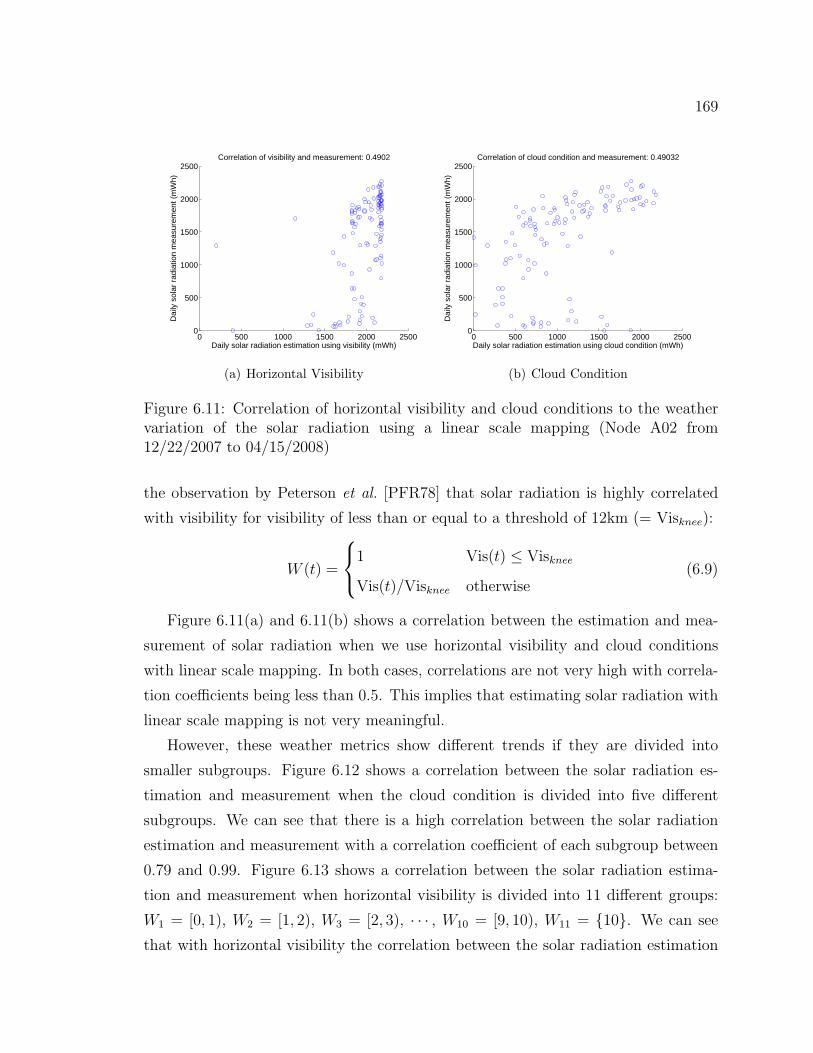
169

0 500 1000 1500 2000 25000

500

1000

1500

2000

2500

Daily solar radiation estimation using visibility (mWh)

Dai

ly s

olar

rad

iatio

n m

easu

rem

ent (

mW

h)

Correlation of visibility and measurement: 0.4902

(a) Horizontal Visibility

0 500 1000 1500 2000 25000

500

1000

1500

2000

2500

Daily solar radiation estimation using cloud condition (mWh)

Dai

ly s

olar

rad

iatio

n m

easu

rem

ent (

mW

h)

Correlation of cloud condition and measurement: 0.49032

(b) Cloud Condition

Figure 6.11: Correlation of horizontal visibility and cloud conditions to the weathervariation of the solar radiation using a linear scale mapping (Node A02 from12/22/2007 to 04/15/2008)

the observation by Peterson et al. [PFR78] that solar radiation is highly correlated

with visibility for visibility of less than or equal to a threshold of 12km (= Visknee):

W (t) =

1 Vis(t) ≤ Visknee

Vis(t)/Visknee otherwise(6.9)

Figure 6.11(a) and 6.11(b) shows a correlation between the estimation and mea-

surement of solar radiation when we use horizontal visibility and cloud conditions

with linear scale mapping. In both cases, correlations are not very high with correla-

tion coefficients being less than 0.5. This implies that estimating solar radiation with

linear scale mapping is not very meaningful.

However, these weather metrics show different trends if they are divided into

smaller subgroups. Figure 6.12 shows a correlation between the solar radiation es-

timation and measurement when the cloud condition is divided into five different

subgroups. We can see that there is a high correlation between the solar radiation

estimation and measurement with a correlation coefficient of each subgroup between

0.79 and 0.99. Figure 6.13 shows a correlation between the solar radiation estima-

tion and measurement when horizontal visibility is divided into 11 different groups:

W1 = [0, 1), W2 = [1, 2), W3 = [2, 3), · · · , W10 = [9, 10), W11 = {10}. We can see

that with horizontal visibility the correlation between the solar radiation estimation

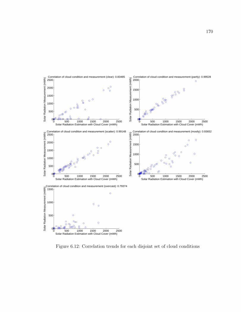
170

0 500 1000 1500 2000 25000

500

1000

1500

2000

2500

Solar Radiation Estimation with Cloud Cover (mWh)

Sol

ar R

adia

tion

Mea

sure

men

t (m

Wh)

Correlation of cloud condition and measurement (clear): 0.83485

0 500 1000 1500 2000 25000

500

1000

1500

2000


Sol

ar R

adia

tion

Mea

sure

men

t (m

Wh)

Correlation of cloud condition and measurement (partly): 0.99528

0 500 1000 1500 2000 25000

500

1000

1500

2000

2500


Sol

ar R

adia

tion

Mea

sure

men

t (m

Wh)

Correlation of cloud condition and measurement (scatter): 0.99148

0 500 1000 1500 2000 25000

500

1000

1500

2000


Sol

ar R

adia

tion

Mea

sure

men

t (m

Wh)

Correlation of cloud condition and measurement (mostly): 0.93652

0 500 1000 1500 2000 25000

500

1000

1500


Sol

ar R

adia

tion

Mea

sure

men

t (m

Wh)

Correlation of cloud condition and measurement (overcast): 0.79374

Figure 6.12: Correlation trends for each disjoint set of cloud conditions

171

0 20 40 60 800

20

40

60

80

Solar radiation estimation with visibility (mWh)

Sol

ar r

adia

tion

mea

sure

men

t (m

Wh)

Correlation for subgroup 1: 0.29578

0 50 1000

20

40

60

80

Solar radiation estimation with visibility (mWh)S

olar

rad

iatio

n m

easu

rem

ent (

mW

h)


0 50 1000

20

40

60

80


Sol

ar r

adia

tion

mea

sure

men

t (m

Wh)


0 50 1000

20

40

60

80


Sol

ar r

adia

tion

mea

sure

men

t (m

Wh)


0 50 1000

10

20

30

40

50


Sol

ar r

adia

tion

mea

sure

men

t (m

Wh)


0 50 1000

20

40

60

80


Sol

ar r

adia

tion

mea

sure

men

t (m

Wh)


0 50 1000

20

40

60

80

100


Sol

ar r

adia

tion

mea

sure

men

t (m

Wh)


0 50 1000

20

40

60

80

100


Sol

ar r

adia

tion

mea

sure

men

t (m

Wh)


0 50 1000

20

40

60

80


Sol

ar r

adia

tion

mea

sure

men

t (m

Wh)


0 50 1000

20

40

60

80


Sol

ar r

adia

tion

mea

sure

men

t (m

Wh)


0 50 1000

20

40

60

80

100


Sol

ar r

adia

tion

mea

sure

men

t (m

Wh)


Figure 6.13: Correlation trends for each disjoint set of visibility

172

0 1 2 3 4 5 6 7 8 9 100

500

1000

1500

2000

2500

3000

3500

4000

4500

5000

Visibility (miles)

Occ

urre

nces

Histogram of occurrences of visibility (k = 11)

Figure 6.14: Occurences (frequency) of each disjoint set of visibility

and measurement is low except for the group with the highest visibility, W11, which

has a correlation coefficient of 0.7. While horizontal visibility has a low correlation

for groups with lower visibility, the histogram in Figure 6.14 shows that groups with

low correlation is insignificant in terms of occurences.

6.3.2 Calibrating Solar Radiation Estimators

We have shown that we can achieve a relatively high correlation between the solar

radiation estimation and measurement by dividing a weather metric into multiple

subgroups. Since a weather metric has a different correlation coefficient depending

on which subgroup it belongs to, the weather factor also needs to be defined for each

subgroup.

The weather factor W (t) can be calibrated using the probability distribution of

the ratio between measurements and estimations for sample points of each subgroup.

Suppose

• The values of weather metrics can be partitioned into k-disjoint subsets W1,

173

W2, · · · , Wk.

• ri, the ratio of the solar radiation measurements over solar radiation estimations

using an obstructed astronomical model for subset Wi on day n, is given by

ri(n) =Yi(n)

Xi(n)=

∫W (t)∈Wi

M(n, t)dt∫W (t)∈Wi

AST (n, t)dt(6.10)

• ri’s belong to [0, rmax], and the set of ri’s, {ri}, is divided into (m+ 1) equally-

spaced bins B0, B1, · · · , Bj, · · · , Bm, where

Bj = { YiXi

| jm· rmax ≤

YiXi

<j + 1

m· rmax} for j = 0, · · · , (m− 1)

Bm = { YiXi

| YiXi

≥ rmax} for j = m (6.11)

Then, the probability that the ratio ri belongs to a bin Bj is

P (ri ∈ Bj) =|Bj||Ball|

(6.12)

where Ball is a union of B0 through Bm. As a calibration factor, we use the expectation

of ri, E(ri) for each subset Wi.

We can describe this process in a more concrete way for cloud conditions and

visibility. For cloud conditions, the k-disjoint subsets can be defined as follows:

W1 = {clear} (6.13)

W2 = {partly cloudy}

W3 = {scatter clouds}

W4 = {mostly cloudy}

W5 = {overcast}

A set of (Xi, Yi) pairs for subset i are the (x,y) coordinates in i-th scatter plot of

Figure 6.12. If we partition a set { Yi

Xi} into 21 bins over domain [0, 2], then we can get a

probability distribution as shown in Figure 6.15. Figure 6.15 also shows that the mean

value of Yi

Xifor each subset. The overall trend is that the calibration factor becomes

smaller as weather becomes more overcast. One exception is the calibration factor

174

for the clear condition. The calculation from the sample points gives a calibration

factor of 0.5341. Since we expect calibration factors to be monitonically descreasing

as cloud conditions become more overcast, we set the calibration factor for the clear

condition as 0.9683, which is the calibration factor for the partly cloudy condition.

For horizontal visibility, which is a real number between 0 and 10, k-disjoint

subsets can be defined by partitioning the domain as follows:

W1 =

[0,

10

k − 1

)(6.14)

W2 =

[10

k − 1,

20

k − 1

)W3 =

[20

k − 1,

30

k − 1

)...

Wk−1 =

[10 · (k − 2)

k − 1,10 · (k − 1)

k − 1

)Wk = {10}

If we consider possible values for k = 11, k-disjoint sets can be given as follows: [0, 1),

[1, 2), [2, 3), · · · , [9, 10), {10}.A set of (Xi, Yi) pairs for subset i are plotted in i-th scatter plot of Figure 6.13. If

we partition a set of { Yi

Xi} into 21 bins over domain [0, 2], then we can get a probability

distribution as shown in Figure 6.16. As a calibration factor for each subset Wi, we

can use the expectation of Yi

Xi, which is shown as a vertical line in each subplot. Since

horizontal visibility is given as a real number between 0 and 10 rather than a discrete

set of numbers, the calibration factor should be a continuous calibration function.

The desirable properties for a calibration function are to minimize the difference be-

tween the measurements and the estimations of solar radiation and to monotonically

increase as horizontal visibility increases. We have considered an exponential curve

and a polynomical curve as a possible calibration function, and curve fitting with

measurements and estimations of solar radiation at the Valley Life Science Building

deployment has shown that an exponential curve is the best candidate. The expo-

nential calibration function that converts a given horizontal visibility x to a number

175

0 0.5 1 1.5 20

0.05

0.1

0.15

0.2

Probability distribution of measurement overestimation ratio for cloud condition (clear)

Mean: 0.5341

0 0.5 1 1.5 20

0.05

0.1

0.15

0.2

Probability distribution of measurement overestimation ratio for cloud condition (partly)

Mean: 0.9683

0 0.5 1 1.5 20

0.05

0.1

0.15

0.2

Probability distribution of measurement overestimation ratio for cloud condition (scatter)

Mean: 0.88

0 0.5 1 1.5 20

0.05

0.1

0.15

0.2

Probability distribution of measurement overestimation ratio for cloud condition (mostly)

Mean: 0.577

0 0.5 1 1.5 20

0.05

0.1

0.15

0.2

Probability distribution of measurement overestimation ratio for cloud condition (overcast)

Mean: 0.1615

c1 c2 c3 c4 c5

Calibration factor 0.9683 0.0983 0.8800 0.5770 0.1615

Figure 6.15: Probability distribution of calibration factor for each disjoint set of cloudconditions

176

y ∈ [0, 1] is given as follows:

y = a · exp(b · x) a : 0.06759 and b : 0.2324 (6.15)

Figure 6.17 shows this exponential calibration function.

6.3.3 Predicting Solar Radiation using the History of a Weather

Effect Component

We have shown how to estimate solar radiation using a weather metric and how to

calibrate such a solar radiation estimator when a sample of measurements are given

for solar radiation and the weather metrics. However, these measurements of solar

radiation and weather metrics are given only for the past and the present. In order

to predict solar radiation under a weather effect for the future, we need a different

model.

A possible model is to predict solar radiation using a recent history of weather

metrics. Figure 6.18 shows an algorithm that estimates the solar radiation for day

n using the astronomical model and the recent k-day history of weather metrics.

As a weather factor for day n, this algorithm uses the ratio of RW HIST(n) and

AST HIST(n), which are the recent k-day average of the solar radiation estimation

using the weather effect and solar radiation estimation using an obstructed astronom-

ical model. At the end of each iteration, the algorithm calculates RW(n), which is the

solar radiation estimation using a weather effect for day n, and updates the history

file with RW(n) so that a later iteration can look it up as history.

We estimated solar radiation using the cloud-based model and the visibility-based

model for the nodes in the VLSB deployment. Figures 6.19 and 6.20 show the trend

of solar radiation prediction with the models with different window sizes (1, 3, 7 and

30 days). Figure 6.21 shows the trend of the deviation between the prediction and

the measurement as we increase the window size. We can see that the deviation is

relatively high with a window size of 1 day, but it stabilizes after 3 days and converges

after 7 days.

Table 6.4 shows the deviation of the prediction from the measurement when we

use a window size of 3 and 7 days. We can see that with the cloud-based model, we

can estimate the trend of solar radiation within 6% of the measured value whereas

177

0 1 20

0.2

0.4

0.6

0.8

Probability distribution of ratio ofmeasurement over estimation for W

1

Mean: 0.4585

0 1 20

0.2

0.4

0.6

0.8


2

Mean: 0.2069

0 1 20

0.2

0.4

0.6

0.8


3

Mean: 0.1267

0 1 20

0.2

0.4

0.6

0.8


4

Mean: 0.1378

0 1 20

0.2

0.4

0.6

0.8


5

Mean: 0.09608

0 1 20

0.2

0.4

0.6

0.8


6

Mean: 0.1467

0 1 20

0.2

0.4

0.6

0.8


7

Mean: 0.3412

0 1 20

0.2

0.4

0.6

0.8


8

Mean: 0.3289

0 1 20

0.2

0.4

0.6

0.8


9

Mean: 0.2732

0 1 20

0.2

0.4

0.6

0.8


10

Mean: 0.5509

0 1 20

0.2

0.4

0.6

0.8


11

Mean: 0.693

Figure 6.16: Probability distribution of calibration factor for each disjoint set ofvisibility

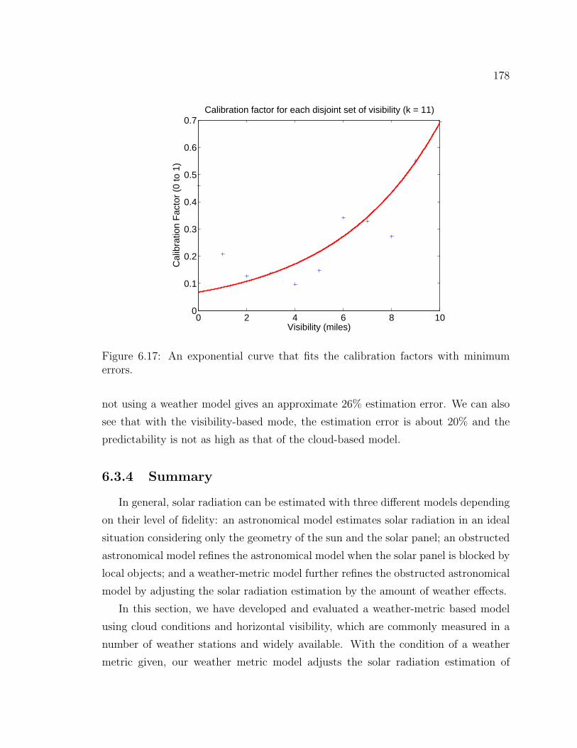
178

0 2 4 6 8 100

0.1

0.2

0.3

0.4

0.5

0.6

0.7

Visibility (miles)

Cal

ibra

tion

Fac

tor

(0 to

1)

Calibration factor for each disjoint set of visibility (k = 11)

Figure 6.17: An exponential curve that fits the calibration factors with minimumerrors.

not using a weather model gives an approximate 26% estimation error. We can also

see that with the visibility-based mode, the estimation error is about 20% and the

predictability is not as high as that of the cloud-based model.

6.3.4 Summary

In general, solar radiation can be estimated with three different models depending

on their level of fidelity: an astronomical model estimates solar radiation in an ideal

situation considering only the geometry of the sun and the solar panel; an obstructed

astronomical model refines the astronomical model when the solar panel is blocked by

local objects; and a weather-metric model further refines the obstructed astronomical

model by adjusting the solar radiation estimation by the amount of weather effects.

In this section, we have developed and evaluated a weather-metric based model

using cloud conditions and horizontal visibility, which are commonly measured in a

number of weather stations and widely available. With the condition of a weather

metric given, our weather metric model adjusts the solar radiation estimation of

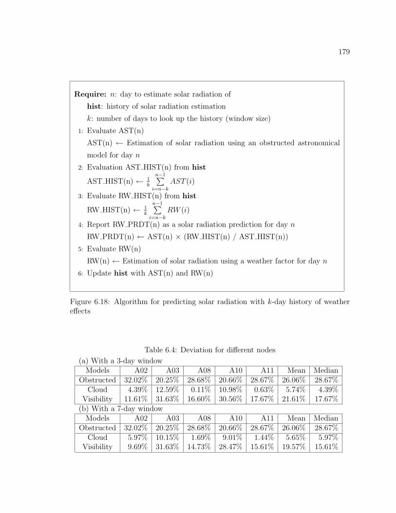
179

Require: n: day to estimate solar radiation of

hist: history of solar radiation estimation

k: number of days to look up the history (window size)

1: Evaluate AST(n)

AST(n) ← Estimation of solar radiation using an obstructed astronomical

model for day n

2: Evaluation AST HIST(n) from hist

AST HIST(n) ← 1k

n−1∑i=n−k

AST (i)

3: Evaluate RW HIST(n) from hist

RW HIST(n) ← 1k

n−1∑i=n−k

RW (i)

4: Report RW PRDT(n) as a solar radiation prediction for day n

RW PRDT(n) ← AST(n) × (RW HIST(n) / AST HIST(n))

5: Evaluate RW(n)

RW(n) ← Estimation of solar radiation using a weather factor for day n

6: Update hist with AST(n) and RW(n)

Figure 6.18: Algorithm for predicting solar radiation with k-day history of weathereffects

Table 6.4: Deviation for different nodes

(a) With a 3-day windowModels A02 A03 A08 A10 A11 Mean Median

Obstructed 32.02% 20.25% 28.68% 20.66% 28.67% 26.06% 28.67%Cloud 4.39% 12.59% 0.11% 10.98% 0.63% 5.74% 4.39%

Visibility 11.61% 31.63% 16.60% 30.56% 17.67% 21.61% 17.67%(b) With a 7-day window

Models A02 A03 A08 A10 A11 Mean MedianObstructed 32.02% 20.25% 28.68% 20.66% 28.67% 26.06% 28.67%

Cloud 5.97% 10.15% 1.69% 9.01% 1.44% 5.65% 5.97%Visibility 9.69% 31.63% 14.73% 28.47% 15.61% 19.57% 15.61%

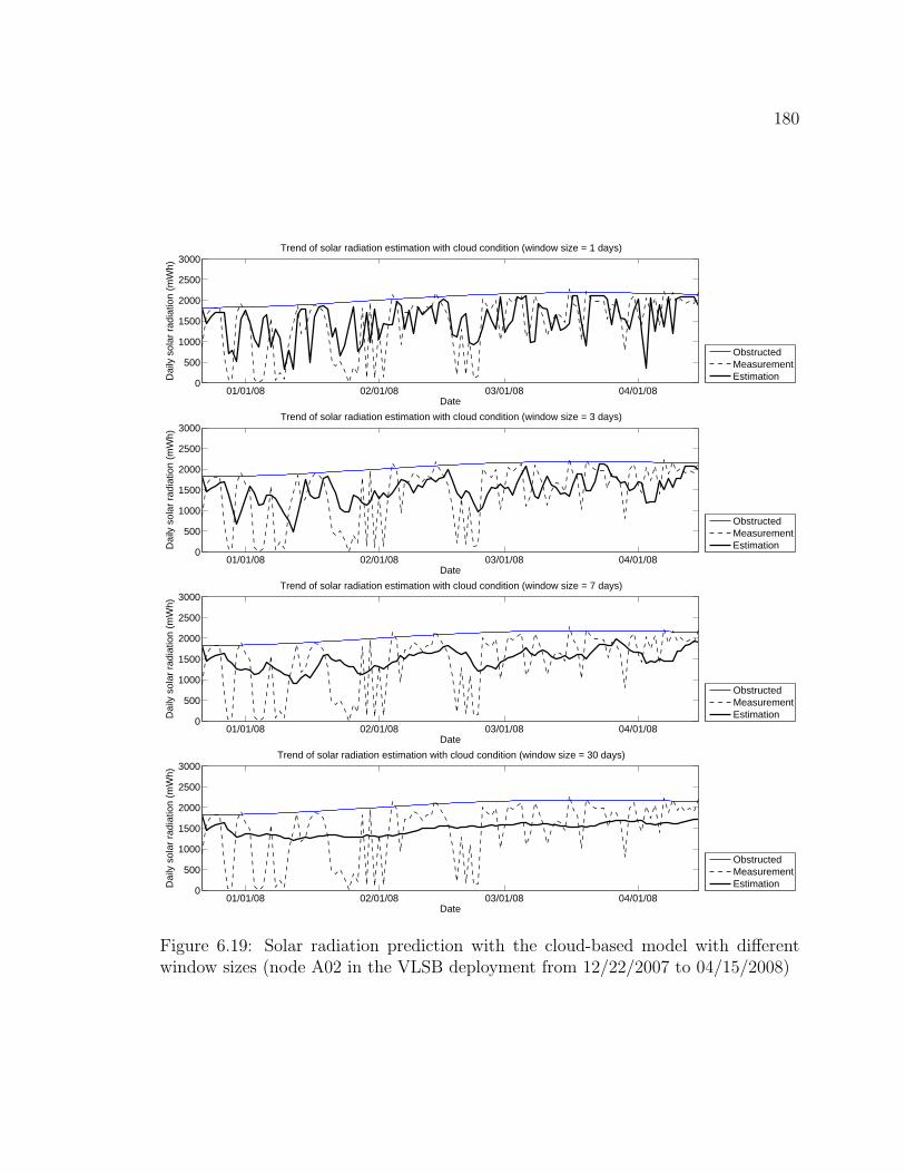
180

01/01/08 02/01/08 03/01/08 04/01/080

500

1000

1500

2000

2500

3000

Date

Dai

ly s

olar

rad

iatio

n (m

Wh)

Trend of solar radiation estimation with cloud condition (window size = 1 days)

ObstructedMeasurementEstimation

01/01/08 02/01/08 03/01/08 04/01/080

1000

2000

3000

Date

Dai

ly s

olar

rad

iatio

n (m

Wh)

Trend of solar radiation estimation with visibility (window size = 1 days)


01/01/08 02/01/08 03/01/08 04/01/080

500

1000

1500

2000

2500

3000

Date

Dai

ly s

olar

rad

iatio

n (m

Wh)



01/01/08 02/01/08 03/01/08 04/01/080

1000

2000

3000

Date

Dai

ly s

olar

rad

iatio

n (m

Wh)



01/01/08 02/01/08 03/01/08 04/01/080

500

1000

1500

2000

2500

3000

Date

Dai

ly s

olar

rad

iatio

n (m

Wh)



01/01/08 02/01/08 03/01/08 04/01/080

1000

2000

3000

Date

Dai

ly s

olar

rad

iatio

n (m

Wh)



01/01/08 02/01/08 03/01/08 04/01/080

500

1000

1500

2000

2500

3000

Date

Dai

ly s

olar

rad

iatio

n (m

Wh)



01/01/08 02/01/08 03/01/08 04/01/080

1000

2000

3000

Date

Dai

ly s

olar

rad

iatio

n (m

Wh)



Figure 6.19: Solar radiation prediction with the cloud-based model with differentwindow sizes (node A02 in the VLSB deployment from 12/22/2007 to 04/15/2008)

181

01/01/08 02/01/08 03/01/08 04/01/080

500

1000

1500

2000

2500

3000

Date

Dai

ly s

olar

rad

iatio

n (m

Wh)



01/01/08 02/01/08 03/01/08 04/01/080

1000

2000

3000

Date

Dai

ly s

olar

rad

iatio

n (m

Wh)



01/01/08 02/01/08 03/01/08 04/01/080

500

1000

1500

2000

2500

3000

Date

Dai

ly s

olar

rad

iatio

n (m

Wh)



01/01/08 02/01/08 03/01/08 04/01/080

1000

2000

3000

Date

Dai

ly s

olar

rad

iatio

n (m

Wh)


ObstructedMeasurementEstimation01/01/08 02/01/08 03/01/08 04/01/08

0

500

1000

1500

2000

2500

3000

Date

Dai

ly s

olar

rad

iatio

n (m

Wh)



01/01/08 02/01/08 03/01/08 04/01/080

1000

2000

3000

Date

Dai

ly s

olar

rad

iatio

n (m

Wh)



01/01/08 02/01/08 03/01/08 04/01/080

500

1000

1500

2000

2500

3000

Date

Dai

ly s

olar

rad

iatio

n (m

Wh)



01/01/08 02/01/08 03/01/08 04/01/080

1000

2000

3000

Date

Dai

ly s

olar

rad

iatio

n (m

Wh)



Figure 6.20: Solar radiation prediction with the visibility-based model with differentwindow sizes (node A02 in the VLSB deployment from 12/22/2007 to 04/15/2008)

182

0 5 10 15 20 25 300

5

10

15

20

25

Window size (days)

Dev

iatio

n fr

om m

easu

rem

ent (

%)

Deviation of cloud−based solar radiation prediction

A02A03A08A10A11

0 5 10 15 20 25 300

10

20

30

40

50

Window size (days)

Dev

iatio

n fr

om m

easu

rem

ent (

%)

Deviation of visibility−based solar radiation prediction

A02A03A08A10A11

Figure 6.21: Deviation of solar radiation prediction with cloud-based and visibility-based models

183

an obstructed astronomical model using the probability distribution of the weather

metric, which is built with samples of the solar radiation measurement and weather

metric.

With the weather-metric model, we predicted the solar radiation by using a k-day

history of the weather metric. With a cloud-based model, we were able to predict the

solar radiation with a 6% margin of error while maintaining 3 or 7 days of history of

the weather metric, while the prediction error is about 26% without a weather metric.

With a visibility-based model, the prediction error was around 20%.

One limitation of this weather-metric based model is that the prediction is for

the average behavior over a certain window of time not for the behavior at a specific

time. This is because our weather-metric model is a probabilistic model and the exact

pattern of the weather metric for the future is not known.

184

Chapter 7

Extending the Simulator Beyond

the Reference Design

In previous chapters, a simulation model of micro-solar power systems was de-

veloped and validated. However, it is not just limited to the reference platform, as

a simulation tool should be able to model hypothetical designs of micro-solar power

systems and predict their behavior. First, this chapter extends the simulation model

for a hypothetical design of micro-solar power systems and demonstrates its utility

(Section 7.1). Then, it discusses possible ideas for extending the simulation model

for two other renewable energy sources: wind and vibrations (Section 7.2).

7.1 Extending the Simulator for a Micro-Solar Power

System with Multi-Level Energy Storage

In earlier chapters of this dissertation, we designed a simulator of the micro-

solar power system and validated it using our reference implementations, one with a

supercapacitor and the other with two AA NiMH batteries. While these two examples

demonstrated that our simulation model can be applied to a micro-solar power system

with energy storage of different types and chemistry, they are demonstrated only

with single-level energy storage. A few designs of micro-solar power system such

as Prometheus [JPC05], Trio [DHJ+06] and AmbiMax [PC06] cannot be directly

simulated with this simulation model.

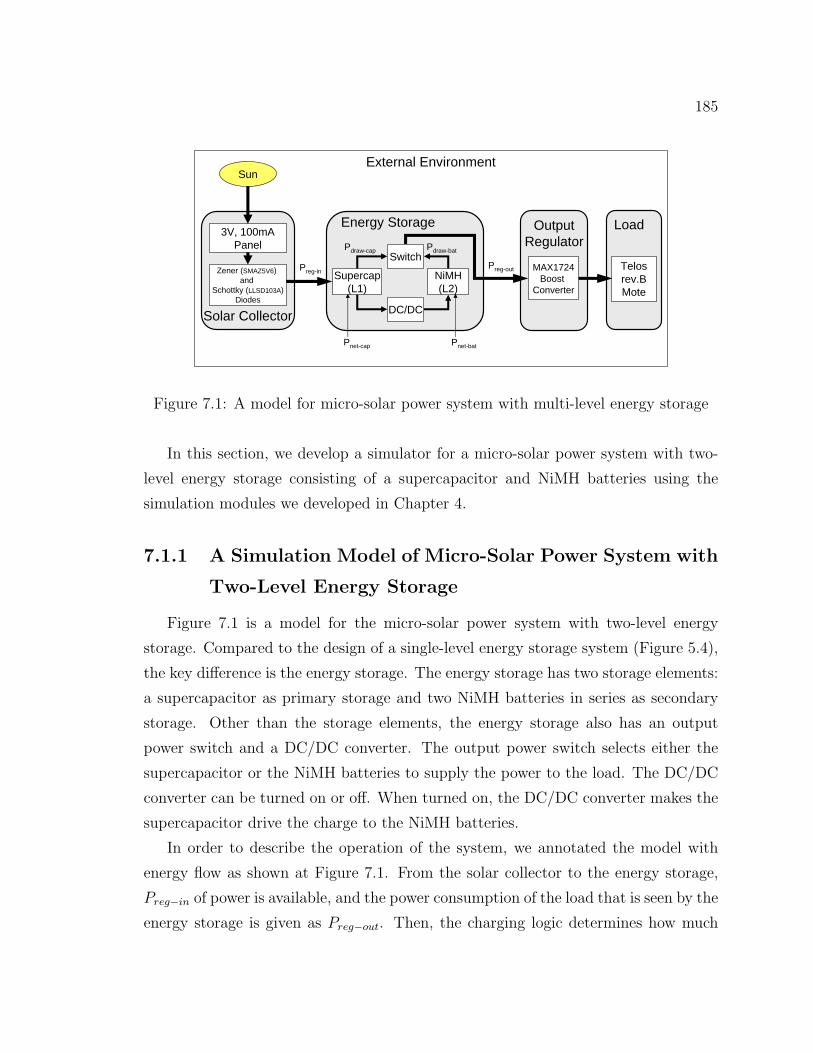
185

OutputRegulator


Load

Telosrev.BMote

3V, 100mAPanel

Zener (SMAZ5V6) and


Supercap(L1)

DC/DC

Sun

NiMH(L2)

Solar Collector

Switch

Energy Storage

MAX1724Boost

Converter

Preg-in

Pnet-bat

Preg-out

Pnet-cap

Pdraw-batPdraw-cap

Figure 7.1: A model for micro-solar power system with multi-level energy storage

In this section, we develop a simulator for a micro-solar power system with two-

level energy storage consisting of a supercapacitor and NiMH batteries using the

simulation modules we developed in Chapter 4.

7.1.1 A Simulation Model of Micro-Solar Power System with

Two-Level Energy Storage

Figure 7.1 is a model for the micro-solar power system with two-level energy

storage. Compared to the design of a single-level energy storage system (Figure 5.4),

the key difference is the energy storage. The energy storage has two storage elements:

a supercapacitor as primary storage and two NiMH batteries in series as secondary

storage. Other than the storage elements, the energy storage also has an output

power switch and a DC/DC converter. The output power switch selects either the

supercapacitor or the NiMH batteries to supply the power to the load. The DC/DC

converter can be turned on or off. When turned on, the DC/DC converter makes the

supercapacitor drive the charge to the NiMH batteries.

In order to describe the operation of the system, we annotated the model with

energy flow as shown at Figure 7.1. From the solar collector to the energy storage,

Preg−in of power is available, and the power consumption of the load that is seen by the

energy storage is given as Preg−out. Then, the charging logic determines how much

186

power can be charged to the supercapacitor and the battery, Pnet−cap and Pnet−bat

respectively. In the rest of this section, we describe the operation of the two-level

energy storage simulator in terms of energy flow of the energy storage elements.

Modeling Each Element of Two-Level Energy Storage

The energy storage elements, supercapacitor and NiMH battery, are simulated

using the variables that represent energy level, voltage, power draw and net charging

power. The output power switch and the DC/DC converter are modeled using discrete

states:

• Supercap:

– Ecap : Energy level of the supercap

– Vcap : Voltage level of the supercap

– Pnet−cap : Net power being charged to the supercap

– Pdraw−cap : Power draw from the supercap

• Battery:

– Ebat : Energy level of the battery

– Vbat : Voltage level of the battery

– Pnet−bat : Net power being charged to the battery

– Pdraw−bat : Power draw from the battery

• Output Power Switch:

– fcap−run : 0 when running on the battery, 1 when on the supercap

• DC/DC Converter:

– fbat−chg : 0 when turned off, 1 when turned on

• Solar Collector:

– Preg−in : Available power from the solar collector

187

– Vsol : Solar panel voltage – positive if the panel is under radiation, 0

otherwise.

• Load and Output Regulator:

– Preg−out : Power draw from the load through the output regulator

The initial conditions for these state variables and other thresholds are listed

below:

• Supercap:

– Ecap−init : Initial energy level of the supercap

– Ecap−max : Maximum energy level of the supercap

– Vcap−lb : Lower bound of the supercap voltage for battery charging

– Vcap−ub : Upper bound of the supercap voltage for battery charging

– Effcap : Efficiency of the supercap

• Battery:

– Ebat−init : Energy level of the battery

– Ebat−max : Voltage level of the battery

– Vbat−lb : Lower bound of the battery voltage for battery charging

– Vbat−ub : Upper bound of the battery voltage for battery charging

– Effcap : Efficiency of the battery

• Output Power Switch:

– fcap−run−init : Initial condition for the output power switch

• DC/DC Converter:

– fbat−chg−init : Initial condition for the DC/DC converter

– Imax−bat−chg : Maximum battery charging current

– Effdc−dc : Efficiency of the DC/DC converter

188

Algorithm for State Transition of Two-Level Energy Storage

The algorithm that determines the state variables of the two-level energy storage

is given at Figure 7.2. While most of the lines are self-explanatory, some of the lines

need explanation:

• Line 10 : The function EtoVbat(), which gives the battery voltage for the

given battery energy level, is described by calc vout NH15 2500() in Fig-

ure 4.19.

• Line 11 : The function EtoVcap(), which gives the supercap voltage for the

given supercap energy level, is described by formula (4.10).

• Line 12 : Formula (4.9) describes the process that evaluates Preg−in[i], which

is the available power from the solar collector.

• Line 14 : The function CalcNetPows() describes the procedure that deter-

mines the net power to the supercap and the battery (Figure 7.3).

• Line 15 : The function CalcFlags() describes the procedure that determines

the discrete states for the output power switch and the DC/DC converter (Fig-

ure 7.5).

CalcNetPows() can be divided into three cases depending on the discrete states

of the output power switch and the DC/DC converter (Figure 7.4):

• Case 1 : Line 2 to 6

In this case, the system runs on the supercapacitor, and the battery is not

being charged. From this condition, the draw from the battery and the net

charge to the battery become zero. The input power from the solar collector

to the supercapacitor is Preg−in, and the draw from the supercapacitor for the

load is Preg−out. From this condition, the power available to the supercapacitor

becomes (Preg−in − Preg−out). We also need to consider that only Effcap of the

available power can be stored due to sub-unity efficiency of the supercap 1.

1The efficiency of the supercapacitor Effcap is modeled as a constant for the sake of simplicity.In a more accurate model, it can be represented as a function of current.

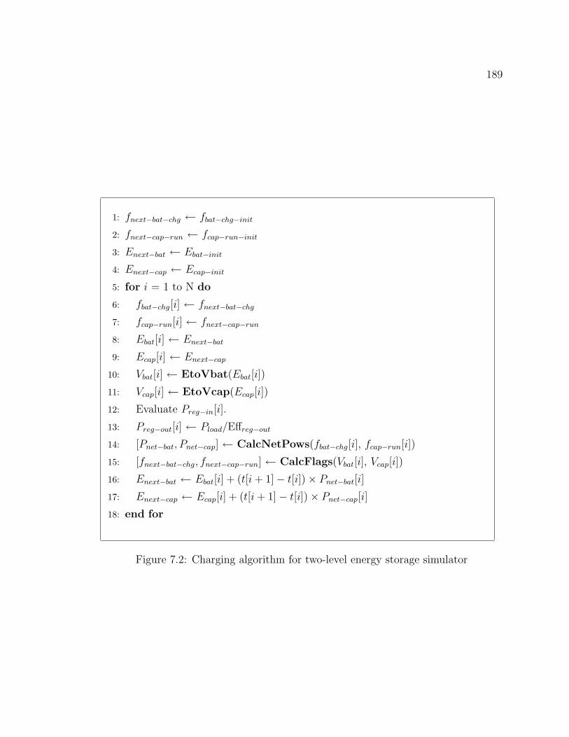
189

1: fnext−bat−chg ← fbat−chg−init

2: fnext−cap−run ← fcap−run−init

3: Enext−bat ← Ebat−init

4: Enext−cap ← Ecap−init

5: for i = 1 to N do

6: fbat−chg[i] ← fnext−bat−chg

7: fcap−run[i] ← fnext−cap−run

8: Ebat[i] ← Enext−bat

9: Ecap[i] ← Enext−cap

10: Vbat[i] ← EtoVbat(Ebat[i])

11: Vcap[i] ← EtoVcap(Ecap[i])

12: Evaluate Preg−in[i].

13: Preg−out[i] ← Pload/Effreg−out

14: [Pnet−bat, Pnet−cap] ← CalcNetPows(fbat−chg[i], fcap−run[i])

15: [fnext−bat−chg, fnext−cap−run] ← CalcFlags(Vbat[i], Vcap[i])

16: Enext−bat ← Ebat[i] + (t[i+ 1]− t[i])× Pnet−bat[i]17: Enext−cap ← Ecap[i] + (t[i+ 1]− t[i])× Pnet−cap[i]18: end for

Figure 7.2: Charging algorithm for two-level energy storage simulator

190

Then, the net charge to the battery and the supercapacitor are as follows:

Pnet−bat = 0 (7.1)

Pnet−cap = (Preg−in − Preg−out)× Effcap (7.2)


In this case, the system runs on the supercapacitor, and the battery is being

charged. The amount of current that flows into the battery is set by the max-

imum battery charge current Imax−bat−chg, which is usually a characteristic of

the DC/DC converter. Thus, the power that is drawn from the supercap is

Vcap × Imax−bat−chg. If we consider that the battery has efficiency factor Effbat

and the DC/DC converter has efficiency factor Effdc−dc, the power that is actu-

ally stored into the battery is the product of the incoming flow, the efficiency

factor of the battery and the efficiency factor of the DC/DC converter. Thus,

the net charge power to the battery and the supercapacitor can be given as

follows:

Pnet−bat = Vcap × Imax−bat−chg × Effbat × Effdc−dc (7.3)

Pnet−cap = (Preg−in − Preg−out)× Effcap − Vcap × Imax−bat−chg (7.4)


In this case, the system runs on the battery, and the battery is not being

charged. The battery has draw of Preg−out with no incoming power, and the

supercapacitor has incoming power of Preg−in with no power draw. Thus, the

net charge power to the battery and the supercapacitor can be given as follows:

Preg−in.

Pnet−bat = −Preg−out (7.5)

Pnet−cap = Preg−in × Effcap (7.6)

The operation of CalcFlags() can be divided depending on the voltage level of

the supercap.

• Stop Charging Condition : Vcap < Vcap−lb

It stops the battery charging. It runs on the battery if the battery voltage is

above the minimum battery voltage. Otherwise, it runs on the supercap.

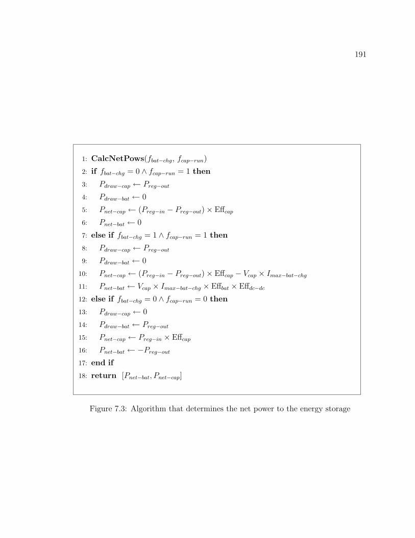
191

1: CalcNetPows(fbat−chg, fcap−run)

2: if fbat−chg = 0 ∧ fcap−run = 1 then

3: Pdraw−cap ← Preg−out

4: Pdraw−bat ← 0

5: Pnet−cap ← (Preg−in − Preg−out)× Effcap

6: Pnet−bat ← 0

7: else if fbat−chg = 1 ∧ fcap−run = 1 then

8: Pdraw−cap ← Preg−out

9: Pdraw−bat ← 0

10: Pnet−cap ← (Preg−in − Preg−out)× Effcap − Vcap × Imax−bat−chg11: Pnet−bat ← Vcap × Imax−bat−chg × Effbat × Effdc−dc

12: else if fbat−chg = 0 ∧ fcap−run = 0 then

13: Pdraw−cap ← 0

14: Pdraw−bat ← Preg−out

15: Pnet−cap ← Preg−in × Effcap

16: Pnet−bat ← −Preg−out17: end if

18: return [Pnet−bat, Pnet−cap]

Figure 7.3: Algorithm that determines the net power to the energy storage

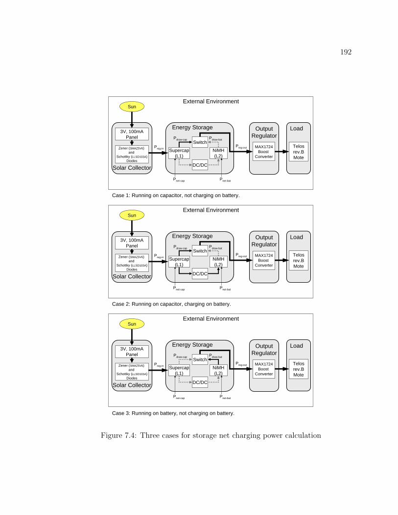
192

OutputRegulator


Load

Telosrev.BMote

3V, 100mAPanel

Zener (SMAZ5V6) and


Supercap(L1)

DC/DC

Sun

NiMH(L2)

Solar Collector

Switch

Energy Storage

MAX1724Boost

Converter

Case 1: Running on capacitor, not charging on battery.

Preg-in

Pnet-bat

Preg-out

Pnet-cap

Pdraw-batPdraw-cap

OutputRegulator


Load

Telosrev.BMote

3V, 100mAPanel

Zener (SMAZ5V6) and


Supercap(L1)

DC/DC

Sun

NiMH(L2)

Solar Collector

Switch

Energy Storage

MAX1724Boost

Converter

Case 2: Running on capacitor, charging on battery.

Preg-in

Pnet-bat

Preg-out

Pnet-cap

Pdraw-batPdraw-cap

OutputRegulator


Load

Telosrev.BMote

3V, 100mAPanel

Zener (SMAZ5V6) and


Supercap(L1)

DC/DC

Sun

NiMH(L2)

Solar Collector

Switch

Energy Storage

MAX1724Boost

Converter

Case 3: Running on battery, not charging on battery.

Preg-in

Pnet-bat

Preg-out

Pnet-cap

Pdraw-batPdraw-cap

Figure 7.4: Three cases for storage net charging power calculation

193

• Start Charging Condition : Vcap ≥ Vcap−lb

It runs on the supercap. It charges the battery if the battery voltage is below

the maximum battery voltage and the solar panel is under radiation. Otherwise,

it stops the battery charging.

• Keep Status Condition : Vcap ≥ Vcap−lb ∧ Vcap < Vcap−ub

It runs on the supercap. It keeps the same charging status if the battery voltage

is below the maximum battery voltage and the solar panel is under radiation.

Otherwise, it stops the battery charging.

7.1.2 Simulation of Micro-Solar Power System with Two-

Level Energy Storage under Constant Radiation

In order to validate the simulation model of the two-level energy storage, we set

up the simulation as follows:

Effect of Storage Size

Two configurations of multi-level energy storage with a supercapacitor and NiMH

batteries are considered by varying the capacity of the supercapacitor (Figure 7.6).

• Configuration 1a : 22F supercap + NiMH

• Configuration 1b : 140F supercap + NiMH

194

1: CalcFlags(Vbat, Vcap)

2: if Vcap < Vcap−lb then

3: fnext−bat−chg ← 0

4: if Vbat ≥ Vbat−lb then

5: fnext−cap−run ← 0

6: else


8: end if

9: else if Vcap ≥ Vcap−lb ∧ Vcap < Vcap−ub then


11: if Vbat ≥ Vbat−ub then


13: else if Vsol > 0 then

14: fnext−bat−chg ← fbat−chg

15: else


17: end if

18: else if Vcap ≥ Vcap−ub then


20: if Vbat ≥ Vbat−ub then


22: else if Vsol > 0 then


24: else


26: end if

27: end if

28: return [fbat−chg, fcap−run]

Figure 7.5: Algorithm that determines the discrete states for the output power switchand the DC/DC converter

195

0 50 100 150 2002

2.2

2.4

2.6

2.8


Vol

tage

(V

)

Cap Voltage (V) : Vcap−lb

= 2.2V, Vcap−ub

= 2.5V

0 50 100 150 20050

55

60

65

70


Ene

rgy

(J)

Cap Energy (J) : capacitance = 22F, Ecap_final

= 68.1947J

0 50 100 150 200

2.5

2.6

2.7

2.8


Vol

tage

(V

)

Bat Voltage (V) : Vbat−lb

= 2.5V, Vbat−ub

= 3V

0 50 100 150 200500

600

700

800


Cap

acity

(m

Ah)

Battery Capacity (mAh) : Effdc−dc

= 80%, Ebat_final

= 797.1912mAh

0 50 100 150 2002.6

2.7

2.8

2.9

3


Vol

tage

(V

)

Solar Panel Voltage

0 50 100 150 20040

50

60

70


Cur

rent

(m

A)

Solar Panel Current

0 50 100 150 200120

140

160

180

Time of Day (Minutes)

Pow

er (

mW

)

Solar Panel Output

0 50 100 150 200−50

0

50

100

150


Pow

er (

mW

)

Net Charge to Storage

(a) Configuration 1a: 22F supercap + NiMH

0 50 100 150 2002

2.2

2.4

2.6

2.8


Vol

tage

(V

)


= 2.2V, Vcap−ub

= 2.5V

0 50 100 150 200300

350

400

450


Ene

rgy

(J)


= 385.7727J

0 50 100 150 200

2.5

2.6

2.7

2.8


Vol

tage

(V

)


= 2.5V, Vbat−ub

= 3V

0 50 100 150 200500

600

700

800

900


Cap

acity

(m

Ah)


= 80%, Ebat_final

= 805.2688mAh

0 50 100 150 2002.6

2.7

2.8

2.9

3


Vol

tage

(V

)

Solar Panel Voltage

0 50 100 150 20040

50

60

70


Cur

rent

(m

A)

Solar Panel Current

0 50 100 150 200120

140

160

180


Pow

er (

mW

)

Solar Panel Output

0 50 100 150 200−50

0

50

100

150


Pow

er (

mW

)


(b) Configuration 1b: 140F supercap + NiMH

Figure 7.6: Effect of storage size

196

The accumulated charge Q = Qbat +Qcap for the two configurations can be calcu-

lated as follows:

For Configuration 1a,

Q = Qbat +Qcap

= (Qbat−final −Qbat−init) +Ecap−final − Ecap−init

3.6J/mWh× Vcap−average

= (797.19mAh− 600mAh) +−0.56J

3.6J/mWh× 2.35V

= 197.10mAh

For Configuration 1b,

Q = Qbat +Qcap

= (Qbat−final −Qbat−init) +Ecap−final − Ecap−init

3.6J/mWh× Vcap−average

= (805.27mAh− 600mAh) +−51.73J

3.6J/mWh× 2.35V

= 199.16mAh

The difference is 1.0% and they accumulate about the same level of charge in the

battery. The difference is the frequency of the charging. For Configuration 1b, which

has a bigger capacitor, it takes a longer time to charge the supercapacitor.

Effect of Supercap Charging Range

Three configurations of multi-level energy storage with a supercapacitor and NiMH

batteries are considered by varying the supercapacitor charging range [Vcap−lb, Vcap−ub]

(Figure 7.7 and Figure 7.8).

• Configuration 2a : 22F supercap + NiMH, Vcap−lb = 2.2V , Vcap−ub = 2.5V

• Configuration 2b : 22F supercap + NiMH, Vcap−lb = 2.3V , Vcap−ub = 2.4V

• Configuration 2c : 22F supercap + NiMH, Vcap−lb = 2.0V , Vcap−ub = 2.3V

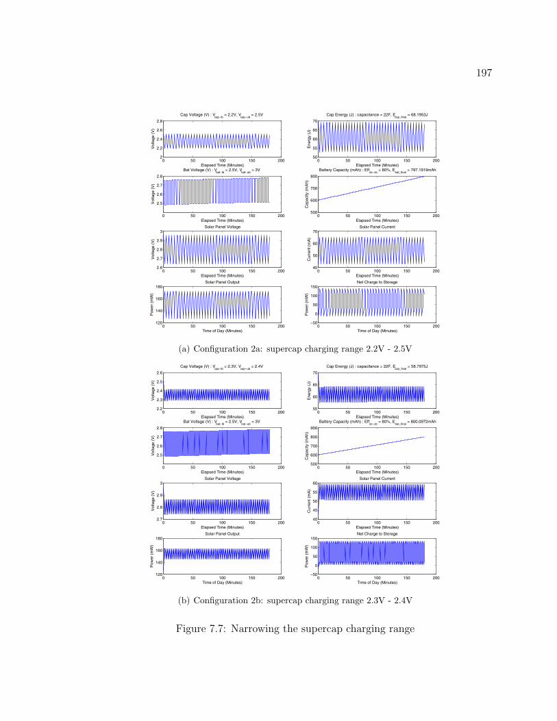
197

0 50 100 150 2002

2.2

2.4

2.6

2.8


Vol

tage

(V

)


= 2.2V, Vcap−ub

= 2.5V

0 50 100 150 20050

55

60

65

70


Ene

rgy

(J)


= 68.1953J

0 50 100 150 200

2.5

2.6

2.7

2.8


Vol

tage

(V

)


= 2.5V, Vbat−ub

= 3V

0 50 100 150 200500

600

700

800


Cap

acity

(m

Ah)


= 80%, Ebat_final

= 797.1919mAh

0 50 100 150 2002.6

2.7

2.8

2.9

3


Vol

tage

(V

)

Solar Panel Voltage

0 50 100 150 20040

50

60

70


Cur

rent

(m

A)

Solar Panel Current

0 50 100 150 200120

140

160

180


Pow

er (

mW

)

Solar Panel Output

0 50 100 150 200−50

0

50

100

150


Pow

er (

mW

)


(a) Configuration 2a: supercap charging range 2.2V - 2.5V

0 50 100 150 2002.2

2.3

2.4

2.5

2.6


Vol

tage

(V

)


= 2.3V, Vcap−ub

= 2.4V

0 50 100 150 20055

60

65

70


Ene

rgy

(J)


= 58.7975J

0 50 100 150 200

2.5

2.6

2.7

2.8


Vol

tage

(V

)


= 2.5V, Vbat−ub

= 3V

0 50 100 150 200500

600

700

800

900


Cap

acity

(m

Ah)


= 80%, Ebat_final

= 800.0972mAh

0 50 100 150 2002.7

2.8

2.9

3


Vol

tage

(V

)

Solar Panel Voltage

0 50 100 150 20040

45

50

55

60


Cur

rent

(m

A)

Solar Panel Current

0 50 100 150 200120

140

160

180


Pow

er (

mW

)

Solar Panel Output

0 50 100 150 200−50

0

50

100

150


Pow

er (

mW

)


(b) Configuration 2b: supercap charging range 2.3V - 2.4V

Figure 7.7: Narrowing the supercap charging range

198

Figure 7.7 compares the effect when the supercapacitor charging range is narrowed

while the center point of the range is the same. The accumulated charge Q for the

two configurations (2a and 2b) are as follows:

For Configuration 2a, Q = Qbat +Qcap = 197.12mAh

For Configuration 2b, Q = Qbat +Qcap = 198.92mAh

In this case, they accumulate the same amount of charge in the battery while the

frequency of charging is different. The one with the narrower range has a higher

frequency of charging.

Figure 7.8 compares the effect when the supercapacitor charging range is shifted

while the width of the range is the same.


For Configuration 2c, Q = Qbat +Qcap = 222.33mAh

In this case, Configuration 2c accumulates 11.3% more charge in the battery than

Configuration 2a. This is because Configuration 2c sets the operating voltage of the

solar panel closer to its maximum power point, as shown in Figure 7.9

Effect of Initial Supercap Voltage Level

Four configurations of multi-level energy storage with a supercapacitor and NiMH

batteries are considered by varying the initial supercapacitor voltage level and the

capacity of the supercapacitor (Figure 7.10 and Figure 7.11).

• Configuration 3a : 22F supercap + NiMH, Vcap−init = 2.5V

• Configuration 3b : 22F supercap + NiMH, Vcap−init = 0.1V

• Configuration 3c : 140F supercap + NiMH, Vcap−init = 2.5V

• Configuration 3d : 140F supercap + NiMH, Vcap−init = 0.1V

199

0 50 100 150 2002

2.2

2.4

2.6

2.8


Vol

tage

(V

)


= 2.2V, Vcap−ub

= 2.5V

0 50 100 150 20050

55

60

65

70


Ene

rgy

(J)


= 68.1953J

0 50 100 150 200

2.5

2.6

2.7

2.8


Vol

tage

(V

)


= 2.5V, Vbat−ub

= 3V

0 50 100 150 200500

600

700

800


Cap

acity

(m

Ah)


= 80%, Ebat_final

= 797.1919mAh

0 50 100 150 2002.6

2.7

2.8

2.9

3


Vol

tage

(V

)

Solar Panel Voltage

0 50 100 150 20040

50

60

70


Cur

rent

(m

A)

Solar Panel Current

0 50 100 150 200120

140

160

180


Pow

er (

mW

)

Solar Panel Output

0 50 100 150 200−50

0

50

100

150


Pow

er (

mW

)


(a) Configuration 2a: supercap charging range 2.2V - 2.5V

0 50 100 150 2001.8

2

2.2

2.4

2.6


Vol

tage

(V

)


= 2V, Vcap−ub

= 2.3V

0 50 100 150 20040

50

60

70


Ene

rgy

(J)


= 53.0196J

0 50 100 150 200

2.5

2.6

2.7

2.8


Vol

tage

(V

)


= 2.5V, Vbat−ub

= 3V

0 50 100 150 200500

600

700

800

900


Cap

acity

(m

Ah)


= 80%, Ebat_final

= 824.3414mAh

0 50 100 150 200

2.6

2.8

3

3.2


Vol

tage

(V

)

Solar Panel Voltage

0 50 100 150 20040

50

60

70

80


Cur

rent

(m

A)

Solar Panel Current

0 50 100 150 200120

140

160

180

200


Pow

er (

mW

)

Solar Panel Output

0 50 100 150 200−50

0

50

100

150


Pow

er (

mW

)


(b) Configuration 2c: supercap charging range 2.0V - 2.3V

Figure 7.8: Shifting the supercap charging range

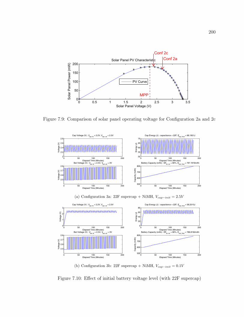
200

0 0.5 1 1.5 2 2.5 3 3.5Solar Panel Voltage (V)

0 0.5 1 1.5 2 2.5 3 3.50

50

100

150

200


Sol

ar P

anel

Pow

er (m

W)


PV Curve

MPP

Conf 2aConf 2c

Figure 7.9: Comparison of solar panel operating voltage for Configuration 2a and 2c

0 50 100 150 2002

2.2

2.4

2.6

2.8


Vol

tage

(V

)


= 2.2V, Vcap−ub

= 2.5V

0 50 100 150 20050

55

60

65

70


Ene

rgy

(J)


= 68.1951J

0 50 100 150 200

2.5

2.6

2.7

2.8


Vol

tage

(V

)


= 2.5V, Vbat−ub

= 3V

0 50 100 150 200500

600

700

800


Cap

acity

(m

Ah)


= 80%, Ebat_final

= 797.1916mAh

0 50 100 150 2002.6

2.7

2.8

2.9

3


Vol

tage

(V

)

Solar Panel Voltage

0 50 100 150 20040

50

60

70


Cur

rent

(m

A)

Solar Panel Current

0 50 100 150 200120

140

160

180


Pow

er (

mW

)

Solar Panel Output

0 50 100 150 200−50

0

50

100

150


Pow

er (

mW

)


(a) Configuration 3a: 22F supercap + NiMH, Vcap−init = 2.5V

0 50 100 150 2000

1

2

3


Vol

tage

(V

)


= 2.2V, Vcap−ub

= 2.5V

0 50 100 150 2000

20

40

60

80


Ene

rgy

(J)


= 58.2515J

0 50 100 150 200

2.5

2.6

2.7

2.8


Vol

tage

(V

)


= 2.5V, Vbat−ub

= 3V

0 50 100 150 200500

600

700

800


Cap

acity

(m

Ah)


= 80%, Ebat_final

= 786.8192mAh

0 50 100 150 2000

1

2

3


Vol

tage

(V

)

Solar Panel Voltage

0 50 100 150 20040

60

80

100

120


Cur

rent

(m

A)

Solar Panel Current

0 50 100 150 20050

100

150

200


Pow

er (

mW

)

Solar Panel Output

0 50 100 150 200−50

0

50

100

150


Pow

er (

mW

)


(b) Configuration 3b: 22F supercap + NiMH, Vcap−init = 0.1V

Figure 7.10: Effect of initial battery voltage level (with 22F supercap)

201

0 50 100 150 2002

2.2

2.4

2.6

2.8


Vol

tage

(V

)


= 2.2V, Vcap−ub

= 2.5V

0 50 100 150 200300

350

400

450


Ene

rgy

(J)


= 385.7725J

0 50 100 150 200

2.5

2.6

2.7

2.8


Vol

tage

(V

)


= 2.5V, Vbat−ub

= 3V

0 50 100 150 200500

600

700

800

900


Cap

acity

(m

Ah)


= 80%, Ebat_final

= 805.2688mAh

0 50 100 150 2002.6

2.7

2.8

2.9

3


Vol

tage

(V

)

Solar Panel Voltage

0 50 100 150 20040

50

60

70


Cur

rent

(m

A)

Solar Panel Current

0 50 100 150 200120

140

160

180


Pow

er (

mW

)

Solar Panel Output

0 50 100 150 200−50

0

50

100

150


Pow

er (

mW

)


(a) Configuration 3c: 140F supercap + NiMH, Vcap−init = 2.5V

0 50 100 150 2000

1

2

3


Vol

tage

(V

)


= 2.2V, Vcap−ub

= 2.5V

0 50 100 150 2000

200

400

600


Ene

rgy

(J)


= 410.9844J

0 50 100 150 200

2.5

2.6

2.7

2.8


Vol

tage

(V

)


= 2.5V, Vbat−ub

= 3V

0 50 100 150 200550

600

650

700

750


Cap

acity

(m

Ah)


= 80%, Ebat_final

= 726.9576mAh

0 50 100 150 2000

1

2

3


Vol

tage

(V

)

Solar Panel Voltage

0 50 100 150 20040

60

80

100

120


Cur

rent

(m

A)

Solar Panel Current

0 50 100 150 20050

100

150

200


Pow

er (

mW

)

Solar Panel Output

0 50 100 150 200−50

0

50

100

150


Pow

er (

mW

)


(b) Configuration 3d: 140F supercap + NiMH, Vcap−init = 0.1V

Figure 7.11: Effect of initial battery voltage level (with 140F supercap)

202

When the supercapacitor is nearly empty (Configuration 3b and 3d), it takes some

amount time before the supercapacitor becomes full (11 minutes for Configuration 3b

and 68 minutes for Configuration 3d). The time it takes to fully charge is proportional

to the capacity of the supercapacitor.

68min/11min = 6.18

140F/22F = 6.36

After the supercapacitor becomes full, it has the same behavior as the one that

started from the full supercapacitor. (Configuration 3a and 3b).

For Configuration 3a,Qfinal −Qcap−full

Tfinal − Tcap−full=

197.19mAh

180min= 1.10mAh/min

For Configuration 3b,Qfinal −Qcap−full

Tfinal − Tcap−full=

186.81mAh

169min= 1.10mAh/min

Effect of Initial Battery Voltage Level


batteries are considered by varying the initial battery voltage level (Figure 7.12).

• Configuration 4a : 22F supercap + NiMH, Ebat−init = 600mAh

• Configuration 4b : 22F supercap + NiMH, Ebat−init = 2000mAh

Configuration 4a and 4b show that the solar panel and the supercapacitor operated

at the same range while transferring the same amount of charge to the battery from

the supercapacitor. The charge accumulation graph shows that the two configurations

accumulated about the same amount of energy:



Effect of Maximum Battery Charging Current

Four configurations of multi-level energy storage with a supercapacitor and NiMH

batteries are considered by varying the maximum battery charging current and the

capacity of the supercapacitor (Figure 7.13 and Figure 7.14).

203

0 50 100 150 2002

2.2

2.4

2.6

2.8


Vol

tage

(V

)


= 2.2V, Vcap−ub

= 2.5V

0 50 100 150 20050

55

60

65

70


Ene

rgy

(J)


= 68.1949J

0 50 100 150 200

2.5

2.6

2.7

2.8


Vol

tage

(V

)


= 2.5V, Vbat−ub

= 3V

0 50 100 150 200500

600

700

800


Cap

acity

(m

Ah)


= 80%, Ebat_final

= 797.1914mAh

0 50 100 150 2002.6

2.7

2.8

2.9

3


Vol

tage

(V

)

Solar Panel Voltage

0 50 100 150 20040

50

60

70


Cur

rent

(m

A)

Solar Panel Current

0 50 100 150 200120

140

160

180


Pow

er (

mW

)

Solar Panel Output

0 50 100 150 200−50

0

50

100

150


Pow

er (

mW

)


(a) Configuration 4a: 22F supercap + NiMH, Ebat−init = 600mAh

0 50 100 150 2002

2.2

2.4

2.6

2.8


Vol

tage

(V

)


= 2.2V, Vcap−ub

= 2.5V

0 50 100 150 20050

55

60

65

70


Ene

rgy

(J)


= 68.1948J

0 50 100 150 2002.5

2.6

2.7

2.8

2.9


Vol

tage

(V

)


= 2.5V, Vbat−ub

= 3V

0 50 100 150 2001900

2000

2100

2200


Cap

acity

(m

Ah)


= 80%, Ebat_final

= 2197.1594mAh

0 50 100 150 2002.6

2.7

2.8

2.9

3


Vol

tage

(V

)

Solar Panel Voltage

0 50 100 150 20040

50

60

70


Cur

rent

(m

A)

Solar Panel Current

0 50 100 150 200120

140

160

180


Pow

er (

mW

)

Solar Panel Output

0 50 100 150 200−50

0

50

100

150


Pow

er (

mW

)


(b) Configuration 4b: 22F supercap + NiMH, Ebat−init = 2000mAh

Figure 7.12: Effect of initial battery voltage level

204

0 50 100 150 2002

2.2

2.4

2.6

2.8


Vol

tage

(V

)


= 2.2V, Vcap−ub

= 2.5V

0 50 100 150 20050

55

60

65

70


Ene

rgy

(J)


= 68.1948J

0 50 100 150 200

2.5

2.6

2.7

2.8


Vol

tage

(V

)


= 2.5V, Vbat−ub

= 3V

0 50 100 150 200500

600

700

800


Cap

acity

(m

Ah)


= 80%, Ebat_final

= 797.1913mAh

0 50 100 150 2002.6

2.7

2.8

2.9

3


Vol

tage

(V

)

Solar Panel Voltage

0 50 100 150 20040

50

60

70


Cur

rent

(m

A)

Solar Panel Current

0 50 100 150 200120

140

160

180


Pow

er (

mW

)

Solar Panel Output

0 50 100 150 200−50

0

50

100

150


Pow

er (

mW

)


(a) Configuration 5a: 22F supercap + NiMH, Imax−bat−chg = 100mA

0 50 100 150 2002

2.2

2.4

2.6

2.8


Vol

tage

(V

)


= 2.2V, Vcap−ub

= 2.5V

0 50 100 150 20040

50

60

70

Elapsed Time (Minutes)E

nerg

y (J

)


= 47.0525J

0 50 100 150 200

2.5

2.6

2.7

2.8


Vol

tage

(V

)


= 2.5V, Vbat−ub

= 3V

0 50 100 150 200500

600

700

800

900


Cap

acity

(m

Ah)


= 80%, Ebat_final

= 804.9702mAh

0 50 100 150 200

2.6

2.8

3

3.2


Vol

tage

(V

)

Solar Panel Voltage

0 50 100 150 20040

50

60

70

80


Cur

rent

(m

A)

Solar Panel Current

0 50 100 150 200120

140

160

180

200


Pow

er (

mW

)

Solar Panel Output

0 50 100 150 200−600

−400

−200

0

200


Pow

er (

mW

)


(b) Configuration 5b: 22F supercap + NiMH, Imax−bat−chg = 500mA

Figure 7.13: Effect of maximum battery charging current (with 22F supercap)

• Configuration 5a : 22F supercap + NiMH, Imax−bat−chg = 100mA

• Configuration 5b : 22F supercap + NiMH, Imax−bat−chg = 500mA

• Configuration 5c : 140F supercap + NiMH, Imax−bat−chg = 100mA

• Configuration 5d : 140F supercap + NiMH, Imax−bat−chg = 500mA

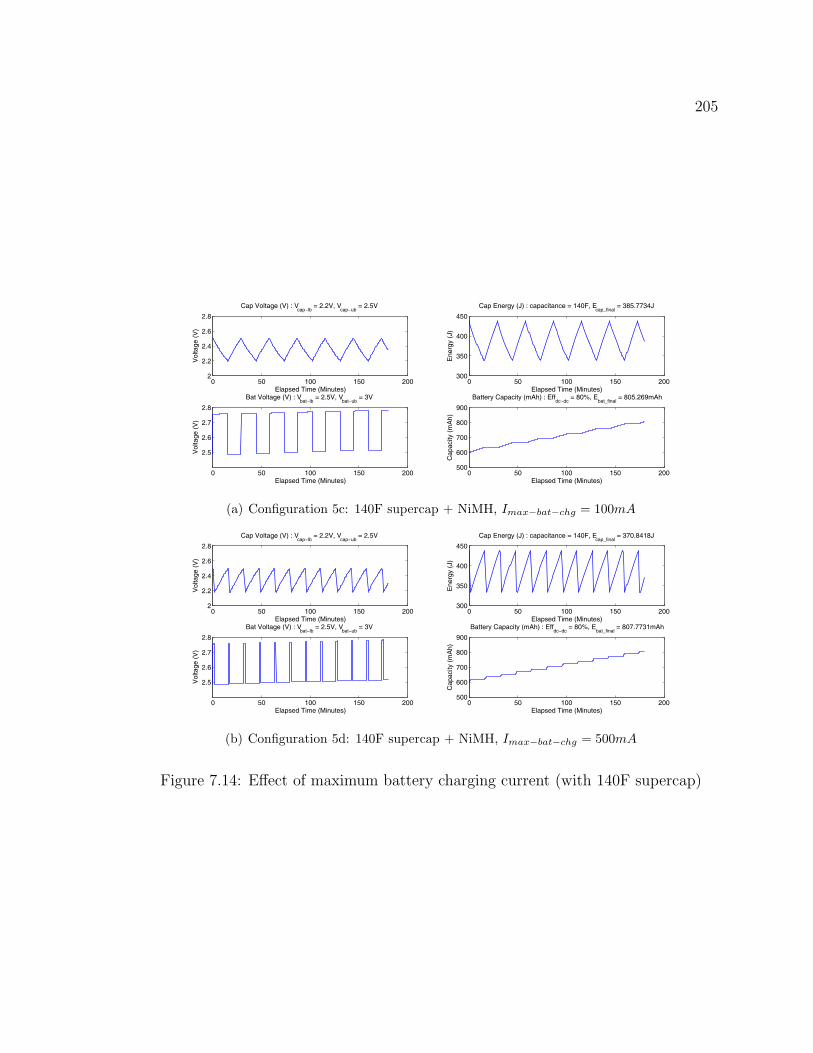
205

0 50 100 150 2002

2.2

2.4

2.6

2.8


Vol

tage

(V

)


= 2.2V, Vcap−ub

= 2.5V

0 50 100 150 200300

350

400

450


Ene

rgy

(J)


= 385.7734J

0 50 100 150 200

2.5

2.6

2.7

2.8


Vol

tage

(V

)


= 2.5V, Vbat−ub

= 3V

0 50 100 150 200500

600

700

800

900


Cap

acity

(m

Ah)


= 80%, Ebat_final

= 805.269mAh

0 50 100 150 2002.6

2.7

2.8

2.9

3


Vol

tage

(V

)

Solar Panel Voltage

0 50 100 150 20040

50

60

70


Cur

rent

(m

A)

Solar Panel Current

0 50 100 150 200120

140

160

180


Pow

er (

mW

)

Solar Panel Output

0 50 100 150 200−50

0

50

100

150


Pow

er (

mW

)


(a) Configuration 5c: 140F supercap + NiMH, Imax−bat−chg = 100mA

0 50 100 150 2002

2.2

2.4

2.6

2.8


Vol

tage

(V

)


= 2.2V, Vcap−ub

= 2.5V

0 50 100 150 200300

350

400

450


Ene

rgy

(J)


= 370.8418J

0 50 100 150 200

2.5

2.6

2.7

2.8


Vol

tage

(V

)


= 2.5V, Vbat−ub

= 3V

0 50 100 150 200500

600

700

800

900


Cap

acity

(m

Ah)


= 80%, Ebat_final

= 807.7731mAh

0 50 100 150 2002.6

2.7

2.8

2.9

3


Vol

tage

(V

)

Solar Panel Voltage

0 50 100 150 20040

50

60

70


Cur

rent

(m

A)

Solar Panel Current

0 50 100 150 200120

140

160

180


Pow

er (

mW

)

Solar Panel Output

0 50 100 150 200−600

−400

−200

0

200


Pow

er (

mW

)


(b) Configuration 5d: 140F supercap + NiMH, Imax−bat−chg = 500mA

Figure 7.14: Effect of maximum battery charging current (with 140F supercap)

206

The accumulated charge in the battery and the supercap are as follows:



For Configuration 5c, Q = Qbat +Qcap = 199.16mAh

For Configuration 5d, Q = Qbat +Qcap = 199.89mAh

We can see that changing the maximum battery charging current does not change

the accumulated charge in the battery and the supercap (2.6% of difference for Con-

figuration 5a and 5b, 0.4% of difference for Configuration 5c and 5d). This is due

to energy conservation. Any charge to the battery through the DC/DC converter is

taken from the supercapacitor, so the overall accumulated charge in the supercapac-

itor is the same. The difference is that the supercapacitor discharge can happen in a

shorter time when the maximum battery charging current increases.

Effect of Efficiency of DC/DC Converter


batteries are considered by varying the efficiency of the DC/DC converter that charges

to the battery (Figure 7.15).

• Configuration 6a : 22F supercap + NiMH, Effdc−dc = 80%

• Configuration 6b : 22F supercap + NiMH, Effdc−dc = 50%

The accumulated charge in the battery and the supercap are as follows:



The efficiency of the DC/DC converter determines what percentage of extra charge

from the supercapacitor can be charged to the battery. We can see that the ratio of

207

0 50 100 150 2002

2.2

2.4

2.6

2.8


Vol

tage

(V

)


= 2.2V, Vcap−ub

= 2.5V

0 50 100 150 20050

55

60

65

70


Ene

rgy

(J)


= 68.195J

0 50 100 150 200

2.5

2.6

2.7

2.8


Vol

tage

(V

)


= 2.5V, Vbat−ub

= 3V

0 50 100 150 200500

600

700

800


Cap

acity

(m

Ah)


= 80%, Ebat_final

= 797.1915mAh

0 50 100 150 2002.6

2.7

2.8

2.9

3


Vol

tage

(V

)

Solar Panel Voltage

0 50 100 150 20040

50

60

70


Cur

rent

(m

A)

Solar Panel Current

0 50 100 150 200120

140

160

180


Pow

er (

mW

)

Solar Panel Output

0 50 100 150 200−50

0

50

100

150


Pow

er (

mW

)


(a) Configuration 6a: 22F supercap + NiMH, Effdc−dc = 80%

0 50 100 150 2002

2.2

2.4

2.6

2.8


Vol

tage

(V

)


= 2.2V, Vcap−ub

= 2.5V

0 50 100 150 20050

55

60

65

70


Ene

rgy

(J)


= 68.1951J

0 50 100 150 200

2.5

2.6

2.7

2.8


Vol

tage

(V

)


= 2.5V, Vbat−ub

= 3V

0 50 100 150 200550

600

650

700

750


Cap

acity

(m

Ah)


= 50%, Ebat_final

= 723.2174mAh

0 50 100 150 2002.6

2.7

2.8

2.9

3


Vol

tage

(V

)

Solar Panel Voltage

0 50 100 150 20040

50

60

70


Cur

rent

(m

A)

Solar Panel Current

0 50 100 150 200120

140

160

180


Pow

er (

mW

)

Solar Panel Output

0 50 100 150 200−100

0

100

200


Pow

er (

mW

)


(b) Configuration 6b: 22F supercap + NiMH, Effdc−dc = 50%

Figure 7.15: Effect of efficiency of DC/DC converter

208

the accumulated charge for the two configurations are almost the same as the ratio

of the efficiency factors of the DC/DC converter:

Q6b/Q6a = 123.16mAh/197.12mAh = 0.6248

Eff6b/Eff6a = 50%/80% = 0.6250

This shows that the accumulated charge is proportional to the efficiency factor of the

DC-DC converter.

Comparison with NiMH-only Storage

A multi-level energy storage with a supercapacitor and NiMH batteries is com-

pared with NiMH-only storage (Figure 7.16).


• Configuration 7b : NiMH

The accumulated charge in the energy storage are as follows:


For Configuration 7b, Q = Qbat = 46.35mAh

We can see that the one with multi-level energy storage accumulates more charge than

the one with the NiMH-only storage. This is because Configuration 7a (22F supercap

+ NiMH) sets the operating point of the solar panel closer to the maximum power

point than Configuration 7b (NiMH only) under the indoor lamp light, as shown in

Figure 7.17.

Operation During Darkness

Two configurations of storage are compared with no radiation. The first one has a

multi-level energy storage with a supercapacitor and the NiMH batteries. The other

is NiMH-only storage (Figure 7.18):


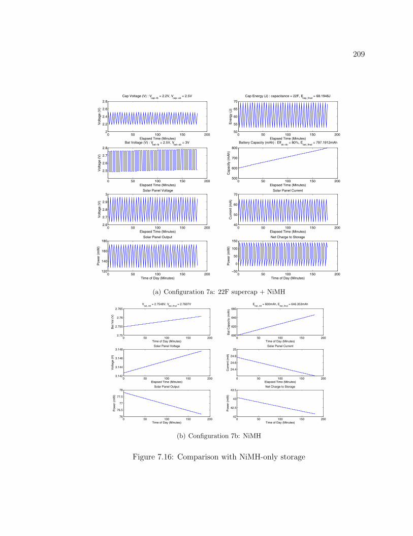
209

0 50 100 150 2002

2.2

2.4

2.6

2.8


Vol

tage

(V

)Cap Voltage (V) : V

cap−lb = 2.2V, V

cap−ub = 2.5V

0 50 100 150 20050

55

60

65

70


Ene

rgy

(J)


= 68.1948J

0 50 100 150 200

2.5

2.6

2.7

2.8


Vol

tage

(V

)


= 2.5V, Vbat−ub

= 3V

0 50 100 150 200500

600

700

800


Cap

acity

(m

Ah)


= 80%, Ebat_final

= 797.1912mAh

0 50 100 150 2002.6

2.7

2.8

2.9

3


Vol

tage

(V

)

Solar Panel Voltage

0 50 100 150 20040

50

60

70

Elapsed Time (Minutes)C

urre

nt (

mA

)

Solar Panel Current

0 50 100 150 200120

140

160

180


Pow

er (

mW

)

Solar Panel Output

0 50 100 150 200−50

0

50

100

150


Pow

er (

mW

)


(a) Configuration 7a: 22F supercap + NiMH0 50 100 150 200

0

20

40

60

80


Pow

er (

mW

)


p = 180, τ = 0.1

0 50 100 150 200

0

0.5

1


0 to

1


= 0.53mA

0 50 100 150 2002.75

2.755

2.76

2.765


Bat

Vol

(V

)

Vbat_init


= 2.7607V

0 50 100 150 200600

620

640

660


Bat

Cap

acity

(m

Ah)

Ebat_init

= 600mAh, Ebat_final

= 646.353mAh

0 50 100 150 2003.142

3.144

3.146

3.148


Vol

tage

(V

)

Solar Panel Voltage

0 50 100 150 200

24.4

24.6

24.8

25


Cur

rent

(m

A)

Solar Panel Current

0 50 100 150 20076

76.5

77

77.5

78


Pow

er (

mW

)

Solar Panel Output

0 50 100 150 20042

42.5

43

43.5


Pow

er (

mW

)


(b) Configuration 7b: NiMH

Figure 7.16: Comparison with NiMH-only storage

210


0 0.5 1 1.5 2 2.5 3 3.50

50

100

150

200


Sol

ar P

anel

Pow

er (m

W)


PV Curve

MPP

Conf 7a

Conf 7b

Figure 7.17: Comparison of solar panel operating voltage for Configuration 7a and7b

0 50 100 150 2001.8

2

2.2

2.4

2.6


Vol

tage

(V

)


= 2.2V, Vcap−ub

= 2.5V

0 50 100 150 20040

50

60

70


Ene

rgy

(J)


= 42.3562J

0 50 100 150 200

2.4824

2.4824

2.4824


Vol

tage

(V

)


= 2.5V, Vbat−ub

= 3V

0 50 100 150 200599.997

599.998

599.999

600

600.001


Cap

acity

(m

Ah)


= 80%, Ebat_final

= 599.9978mAh

0 50 100 150 200−1

−0.5

0

0.5

1


Vol

tage

(V

)

Solar Panel Voltage

0 50 100 150 200−1

−0.5

0

0.5

1


Cur

rent

(m

A)

Solar Panel Current

0 50 100 150 200−1

−0.5

0

0.5

1


Pow

er (

mW

)

Solar Panel Output

0 50 100 150 200−2.3

−2.25

−2.2

−2.15


Pow

er (

mW

)


(a) Configuration 8a: 22F supercap + NiMH0 50 100 150 200

−4

−2

0

2

4


Pow

er (

mW

)


p = 180, τ = 0.1

0 50 100 150 200

0

0.5

1


0 to

1


= 0.53mA

0 50 100 150 2002.4818

2.482

2.4822

2.4824

2.4826


Bat

Vol

(V

)

Vbat_init


= 2.4819V

0 50 100 150 200596

597

598

599

600


Bat

Cap

acity

(m

Ah)

Ebat_init

= 600mAh, Ebat_final

= 596.8339mAh

0 50 100 150 200−1

−0.5

0

0.5

1


Vol

tage

(V

)

Solar Panel Voltage

0 50 100 150 200−1

−0.5

0

0.5

1


Cur

rent

(m

A)

Solar Panel Current

0 50 100 150 200−1

−0.5

0

0.5

1


Pow

er (

mW

)

Solar Panel Output

0 50 100 150 200−2.62

−2.6198

−2.6196

−2.6194

−2.6192


Pow

er (

mW

)


(b) Configuration 8b: NiMH

Figure 7.18: Operation during darkness

211

• Configuration 8b : NiMH

The accumulated charge in the energy storage shows that 3.12mAh and 3.17mAh

of charge was drawn from the storage for each case.

For Configuration 8a, Q = Qbat +Qcap = −3.12mAh

For Configuration 8b, Q = Qbat = −3.17mAh

This result matches the estimated charge consumption of the load through the

output regulator.

Qreg−out = Ireg−out × T ×1

Effreg−out

= 0.53mA× 3hr × 1

0.5

= 3.18mAh

7.1.3 Summary of Simulation of Multi-Level Energy Storage

In this section, we have demonstrated that we are able to simulate a hypothetical

design of a micro-solar power system. As an example of a hypothetical design, we

simulated a micro-solar power system with multi-level energy storage consisting of a

supercapacitor and NiMH batteries. From the simulations, we observed the follow-

ings:

• The supercapacitor charging range affects the amount of charge transfer; more

charge is transferred when the average supercapacitor voltage is matched closer

to the maximum power point of the solar panel.

• The efficiency of the DC/DC converter determines how much charge from the

supercapacitor is transferred to the battery.

• Other initial conditions do not affect the amount of charge transfer. They are

the capacity of the supercapacitor, the width of the supercapacitor charging

range, the initial voltage level of the supercapacitor, and the maximum battery

charging current.

212

We also found that our hypothetical design of a micro-solar power system with

multi-level energy storage had a higher energy transfer rate than the system with

the NiMH-only energy storage. This is because our hypothetical system had better

matching for the maximum power point of the solar panel. While we demonstrated the

case where our hypothetical design performs better than the system with the NiMH-

only energy storage, the simulator can also produce the case where our hypothetical

design performs worse. For example, setting the supercapacitor charging range farther

from the optimum range makes the solar panel output power smaller.

7.2 Extending the Simulator for Other Renewable

Energy Sources

This dissertation has focused on the use of outdoor solar energy for mote-class

devices among various types of renewable energy sources. However, other renewable

energy sources can also be considered in the absence of outdoor solar energy, although

their power density is not as high as that of outdoor sunlight. In this section, we

review two cases of other renewable energy sources – wind and vibrations. For each

type of renewable energy source, we describe the characteristics of the energy source,

the energy collector, and the rest of the energy harvesting system. Then, we will

describe a brief idea on extending the micro-solar power simulator for each renewable

energy source.

7.2.1 Extension for a Wind Energy Harvesting System

A wind energy harvesting system can be represented as a generic model in Fig-

ure 7.19, which consists of the following components: the external environment, an

energy collector, input regulator, energy storage, output regulator, and a load. The

wind energy from the environment is collected by a wind generator. The electricity

generated from the wind generator is AC 2 and it needs to be converted to DC be-

fore it is stored in the energy storage. The input regulator does this conversion: the

2As for wind generator, a three-phase permanent magnet synchronous generator is assumed, butother types of AC generator can be used.

213


EnergyCollector

(WindGenerator)

EnergyStorage

LoadOutputRegulator(Optional)

Wind

Input Regulator

Rectifier DC/DCConverter

Figure 7.19: A generic model for wind energy harvesting system

rectifier converts AC to DC, and the DC-DC converter adjusts the voltage level of

the DC rectifier output to be within the charging range of the energy storage. The

energy stored in the energy storage is used by the load and it can possibly go through

an output regulator.

If we compare this with the architecture of a micro-solar power system, we can

see that a wind energy harvesting system has different characteristics for the external

environment, energy collector and input regulator. In the rest of this section, we will

describe the characteristics of these components.

External Environment: Wind

Based on a fact that power from the wind is proportional to the cube of the wind

speed [GCD+98], we can estimate the energy income by determining the wind speed

at a particular location:

Pwind ∝ V 3wind (7.7)

where the wind speed Vwind can be measured or estimated from previous statistics.

Energy Collector: Wind Generator

The wind generator converts the mechanical energy from the wind to electrical

energy. In order to model and characterize a wind generator, we use the experimental

214

data by Gevorgian et al. [GCD+98] in Figure 7.20. From this experimental data, we

know the followings:

• When the wind speed is between the lower bound (about 3m/s) and the upper

bound (about 8m/s), the relationship between the wind speed and the wind

generator output power follows the cubic curve.

• When the wind speed is above the upper bound, the output power is almost

flat. This is because a wind generator is made not to exceed the maximum

output voltage, which limits the wind generator output power above the upper

bound.

• When the wind speed is below the lower bound, the output power is zero. This

is when the output voltage of the wind generator is lower than the threshold

voltage of the rectifier and is not usable.

From these findings, we can formulate the output of a wind generator as follows:

Pwind−gen = min{max{k · V 3wind − Pth, 0}, Pmax} (7.8)

Input Regulator

The input regulator for the wind energy harvesting system has two components:

a rectifier and a DC-DC converter. We can characterize the input regulator with an

operating range and a power efficiency for the rectifier and DC-DC converter.

Figure 7.21 summarizes the extension for the simulation with wind energy har-

vesting.

7.2.2 Extension for Vibrational Energy Harvesting System

A vibrational energy harvesting system can be represented as a generic model

in Figure 7.22, which is composed of the external environment, an energy collector,

input regulator, energy storage, output regulator, and a load. The vibrational energy

from the environment is collected by the vibration-to-electricity converter. Similar

to the case of wind energy harvesting, the electricity generated from the vibration

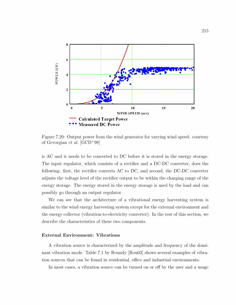
215

Figure 7.20: Output power from the wind generator for varying wind speed: courtesyof Gevorgian et al. [GCD+98]

is AC and it needs to be converted to DC before it is stored in the energy storage.

The input regulator, which consists of a rectifier and a DC-DC converter, does the

following: first, the rectifier converts AC to DC, and second, the DC-DC converter

adjusts the voltage level of the rectifier output to be within the charging range of the

energy storage. The energy stored in the energy storage is used by the load and can

possibly go through an output regulator.

We can see that the architecture of a vibrational energy harvesting system is

similar to the wind energy harvesting system except for the external environment and

the energy collector (vibration-to-electricity converter). In the rest of this section, we

describe the characteristics of these two components.

External Environment: Vibrations

A vibration source is characterized by the amplitude and frequency of the domi-

nant vibration mode. Table 7.1 by Roundy [Rou03] shows several examples of vibra-

tion sources that can be found in residential, office and industrial environments.

In most cases, a vibration source can be turned on or off by the user and a usage

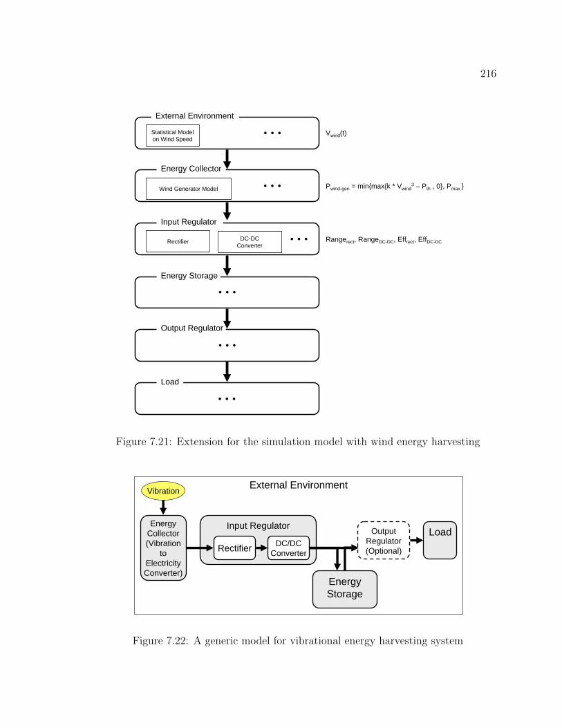
216

DC-DCConverter

Input Regulator

Rectifier …

Energy Collector

Wind Generator Model…


Statistical Modelon Wind Speed

…

Energy Storage

…

Output Regulator

…

Load

…

Vwind(t)

Pwind-gen = min{max{k * Vwind3 – Pth , 0}, Pmax }

Rangerect, RangeDC-DC, Effrect, EffDC-DC

Figure 7.21: Extension for the simulation model with wind energy harvesting


EnergyCollector(Vibration

toElectricityConverter)

EnergyStorage

LoadOutputRegulator(Optional)

Vibration

Input Regulator

Rectifier DC/DCConverter

Figure 7.22: A generic model for vibrational energy harvesting system

217

Table 7.1: List of vibration sources with the characteristics of the dominant vibrationmode – courtesy of Roundy [Rou03]

Vibration Source Acceleration Frequency

(m/s2) (Hz)

Base of 5 HP 3-axis machine tool with 36” bed 10 70

Kitchen blender casing 6.4 121

Clothes dryer 3.5 121

Door frame just after door closes 3 125

Small microwave oven 2.25 121

HVAC vents in office building 0.2 – 1.5 60

Wooden deck with people walking 1.3 385

Breadmaker 1.03 121

External windows (size 2ft x 3ft) next to a busy street 0.7 100

Notebook computer while CD is being read 0.6 75

Washing Machine 0.5 109

Second story floor of a wood frame office building 0.2 100

Refrigerator 0.1 240

pattern needs to be considered. For example, HVAC vents can vibrate in the same

pattern all day long, but they can have different patterns for day and night if air

conditioning is turned off for energy saving during the night.

Energy Collector: Vibration-to-Electricity Converter

According to Roundy [Rou03], the output power of a vibration-to-electricity con-

verter can be formulated as follows when the resonant frequency of the converter

218

matches the frequency of the vibration ω:

|P | = mζeA2

4ωζ2T

(7.9)

m : mass

ω : driving frequency

A : amplitude of acceleration

ζe : damping ratio (electric)

ζT : damping ratio (electric and mechanical)

From this equation, we can see the following: (a) the output power is proportional

to the mass of the converter; (b) the output power is inversely proportional to the

frequency of the driving vibration; (c) the output power is proportional to the square

of the amplitude of the acceleration. The work of Roundy [Rou03] shows a concrete

example of a vibration-to-electricity converter. He demonstrated that a piezo-electric

vibration-to-electricity converter had an energy density of 335uW/cm3 with a vi-

bration source of 2.25m/s2 at 60Hz. Figure 7.23 summarizes the extension for the

simulation with vibrational energy harvesting.

7.3 Summary

In this chapter, we explored two ideas for extending the micro-solar power system

simulator. First, in order to demonstrate that the micro-solar power system simu-

lator can be extended for a hypothetical design, we simulated a micro-solar power

system with a multi-level energy storage consisting of a supercapacitor and NiMH

batteries. From the simulations, we were able to determine which system param-

eters affected the system and how. Second, we extended the simulator to include

wind and vibration energy to demonstrate that the simulation tool can be used for

other renewable energy sources. The extended simulator is organized similarly to the

micro-solar power system simulator: the external environment, an energy collector,

input regulator, energy storage, output regulator, and a load. The differences are the

characteristics of the external environment (e.g. wind and vibration) and the energy

collector (e.g. wind generator and piezo-electric material).

219

DC-DCConverter

Input Regulator

Rectifier …

Energy Collector

Vibration-to-ElectricityConverter Model

…


Statistical Modelon Vibration

…

Energy Storage

…

Output Regulator

…

Load

…

A, ω, rate(t) for the vibration source

Rangerect, RangeDC-DC, Effrect, EffDC-DC

for a generic converter2

2

4||

T

e AmPωζζ

=

For a particular type of converter with

the given A and ω, we can use the energy density.

Figure 7.23: Extension for the simulation model with vibrational energy harvesting

220

Chapter 8

Extending the Simulator for a

Meso-Solar Power System

In this chapter, we extend our simulation tools for a meso-solar system to validate

our model with a solar power system of a larger scale. For this purpose, we design

a solar-powered web server by composing Watt-scale components (Section 8.1). We

simulate this design by building a model for each component and integrating it into

our simulator (Section 8.2). Then, we validate this design against the measurement

of the implementation (Section 8.3) and use this result for long-term prediction (Sec-

tion 8.4).

8.1 System Architecture of Meso-Solar System

The solar-powered web server is a PDA-class Linux box that has an 802.11 wireless

interface and runs a web service (Figure 8.1). This meso-solar system has very similar

components – solar panel, input regulator, energy storage, output regulator and load

– and organization to a micro-solar power system (Figure 8.2). However, the scale

and efficiency numbers are quite different. For example, the solar panel of the solar-

powered web server is rated at 50W, whereas a typical solar panel for a micro-solar

power system has 100mW to 500mW of output power. In the rest of the section, we

look at the details of each component of the solar-powered web server and compare

the numbers with those of a micro-solar power system.

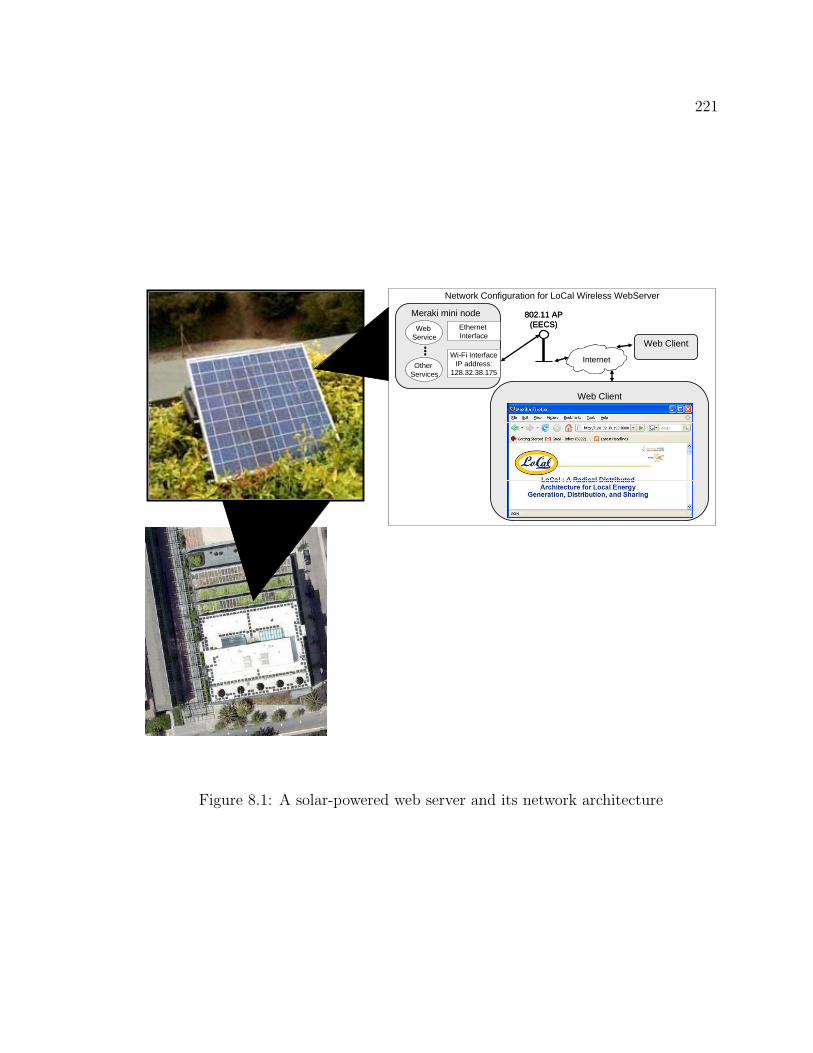
221

Network Configuration for LoCal Wireless WebServer

Web Client

Meraki mini nodeEthernet Interface

Wi-Fi InterfaceIP address:

128.32.38.175

…

Other Services

InternetInternet

802.11 AP(EECS)

802.11 AP(EECS)Web

Service

Web Client

Figure 8.1: A solar-powered web server and its network architecture

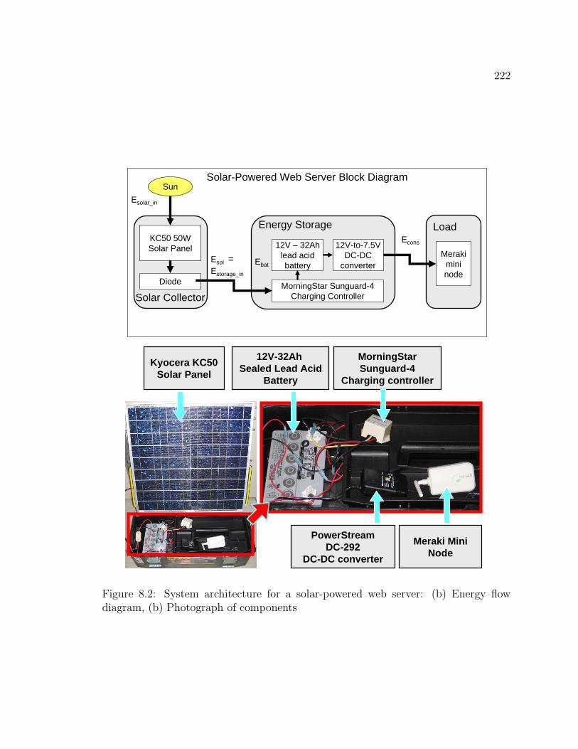
222

Solar-Powered Web Server Block Diagram

Load

Merakimininode

KC50 50WSolar Panel

Diode

12V – 32Ahlead acidbattery

MorningStar Sunguard-4Charging Controller

SunEsolar_in

Estorage_in

Econs

Solar Collector

Energy Storage

12V-to-7.5VDC-DC

converterEsol = Ebat

Kyocera KC50Solar Panel

PowerStreamDC-292

DC-DC converter

MorningStarSunguard-4

Charging controller

Meraki MiniNode

12V-32Ah Sealed Lead Acid

Battery

Figure 8.2: System architecture for a solar-powered web server: (b) Energy flowdiagram, (b) Photograph of components

223

Load: Meraki Mini

A Meraki Mini node [Mer], which is a PDA-class 802.11-wireless capable Linux

box, is used as the load for the solar-powered web server. The power consumption of

a Meraki Mini node provided by the manufacturer is typically 3.5W and at maximum

7.5W. We measured the average power consumption of a Meraki Mini as 2.25W (=

7.5V * 0.3A). In contrast, the HydroWatch application, our reference implementation

for a micro-solar power system, has an average power consumption of 1.5mW, more

than 1000-times smaller than the power consumption of a meso-solar system.

Solar Panel: Kyocera KC50 Panel

The solar panel for the solar-powered web server is a Kyocera KC50 panel [Kyo].

The KC50 panel has a maximum power of 50W at 16.7V with 3.0A and an open-circuit

voltage of 21.5V and a short-circuit current of 3.1A. The I-V and P-V characteristics

of a KC50 panel are shown at Figure 8.3. Whereas, the HydroWatch application has

a maximum of 300mW of solar panel output, which is 100-times smaller than the

solar panel output of the meso-solar system.

Energy Storage: 12V-32Ah Sealed Lead Acid Battery

As energy storage, a sealed-lead acid battery with a nominal operating voltage

of 12V and a capacity of 32Ah was used. The relationship between battery voltage

and capacity is shown in Figure 8.4. This relationship is generated from a voltage-

to-capacity curve of a 12V lead acid battery [Per93] assuming total capacity of 32Ah,

a charging rate of C/20 and a discharging rate of C/100 1. The charge-discharge

efficiency is not shown for this particular model of battery, but it is known that a

lead acid battery has an efficiency of 70% to 92% [Wik].

Input Regulator: MorningStar Sunguard-4

A MorningStar Sunguard-4 charging controller is used as an input regulator. This

charging controller is designed for charging a 12V lead-acid battery with a maximum

1C is the capacity rating of the battery. For example, C/20 is 1/20 of C and C/100 is 1/100 ofC.

224

0 5 10 15 20 250

1000

2000

3000

4000


Sol

ar P

anel

Cur

rent

(m

A)

Solar Panel IV Characteristic (Kyocera KC50)

IV Curve

0 5 10 15 20 250

2

4

6x 10

4


Sol

ar P

anel

Pow

er (

mW

)

Solar Panel PV Characteristic (Kyocera KC50)

PV Curve

Figure 8.3: Characteristic for Kyocera KC50 solar panel. I = Isc−A ·(exp(B ·V )−1)with A = 0.0063, B = 0.6096, Isc = 3100. Units of V and I are V and mA.

0 1 2 3 4

x 104

12

12.5

13

13.5

14

14.5

15

15.5

16

Remaining Charge (mAh)

Vol

tage

(V

)

Charge Characteristic for 12V−32Ah lead acid battery

0 1 2 3 4

x 104

11.8

12

12.2

12.4

12.6

12.8

Used Charge (mAh)

Vol

tage

(V

)

Discharge Characteristic for 12V−32Ah lead acid battery

Figure 8.4: Voltage-to-capacity relationship for 12V-32Ah lead acid battery: (a)charging, (b) discharging

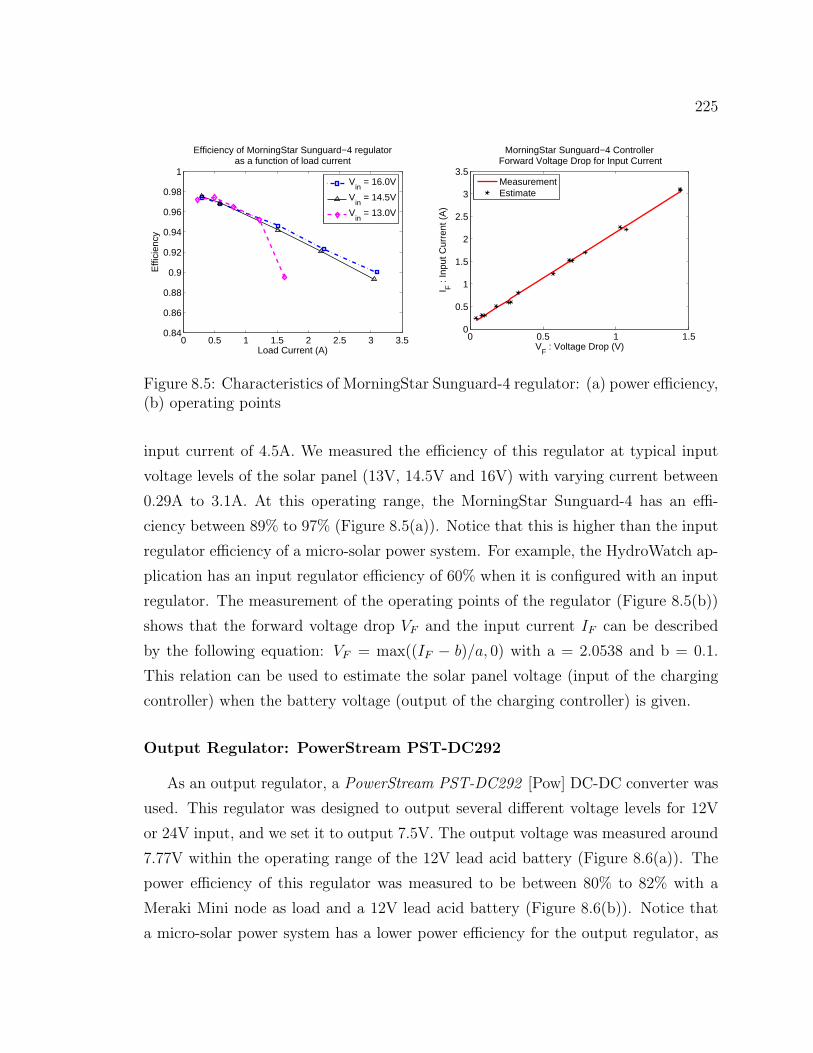
225

0 0.5 1 1.5 2 2.5 3 3.50.84

0.86

0.88

0.9

0.92

0.94

0.96

0.98

1

Load Current (A)

Effi

cien

cyEfficiency of MorningStar Sunguard−4 regulator

as a function of load current

Vin

= 16.0V

Vin

= 14.5V

Vin

= 13.0V

0 0.5 1 1.50

0.5

1

1.5

2

2.5

3

3.5

VF : Voltage Drop (V)

I F :

Inpu

t Cur

rent

(A

)

MorningStar Sunguard−4 ControllerForward Voltage Drop for Input Current

MeasurementEstimate

Figure 8.5: Characteristics of MorningStar Sunguard-4 regulator: (a) power efficiency,(b) operating points

input current of 4.5A. We measured the efficiency of this regulator at typical input

voltage levels of the solar panel (13V, 14.5V and 16V) with varying current between

0.29A to 3.1A. At this operating range, the MorningStar Sunguard-4 has an effi-

ciency between 89% to 97% (Figure 8.5(a)). Notice that this is higher than the input

regulator efficiency of a micro-solar power system. For example, the HydroWatch ap-

plication has an input regulator efficiency of 60% when it is configured with an input

regulator. The measurement of the operating points of the regulator (Figure 8.5(b))

shows that the forward voltage drop VF and the input current IF can be described

by the following equation: VF = max((IF − b)/a, 0) with a = 2.0538 and b = 0.1.

This relation can be used to estimate the solar panel voltage (input of the charging

controller) when the battery voltage (output of the charging controller) is given.

Output Regulator: PowerStream PST-DC292

As an output regulator, a PowerStream PST-DC292 [Pow] DC-DC converter was

used. This regulator was designed to output several different voltage levels for 12V

or 24V input, and we set it to output 7.5V. The output voltage was measured around

7.77V within the operating range of the 12V lead acid battery (Figure 8.6(a)). The

power efficiency of this regulator was measured to be between 80% to 82% with a

Meraki Mini node as load and a 12V lead acid battery (Figure 8.6(b)). Notice that

a micro-solar power system has a lower power efficiency for the output regulator, as

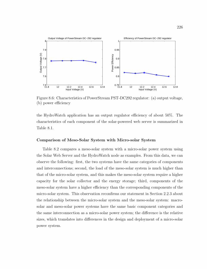
226

11.8 12 12.2 12.4 12.6 12.87.5

7.6

7.7

7.8

7.9

8

Input Voltage (V)

Out

put V

olta

ge (

V)

Output Voltage of PowerStream DC−292 regulator

11.8 12 12.2 12.4 12.6 12.80.75

0.8

0.85

0.9

0.95

1

Input Voltage (V)

Pow

er E

ffici

ency

Efficiency of PowerStream DC−292 regulator

Figure 8.6: Characteristics of PowerStream PST-DC292 regulator: (a) output voltage,(b) power efficiency

the HydroWatch application has an output regulator efficiency of about 50%. The

characteristics of each component of the solar-powered web server is summarized in

Table 8.1.

Comparison of Meso-Solar System with Micro-solar System

Table 8.2 compares a meso-solar system with a micro-solar power system using

the Solar Web Server and the HydroWatch node as examples. From this data, we can

observe the following: first, the two systems have the same categories of components

and interconnections; second, the load of the meso-solar system is much higher than

that of the micro-solar system, and this makes the meso-solar system require a higher

capacity for the solar collector and the energy storage; third, components of the

meso-solar system have a higher efficiency than the corresponding components of the

micro-solar system. This observation reconfirms our statement in Section 2.2.3 about

the relationship between the micro-solar system and the meso-solar system: macro-

solar and meso-solar power systems have the same basic component categories and

the same interconnection as a micro-solar power system; the difference is the relative

sizes, which translates into differences in the design and deployment of a micro-solar

power system.

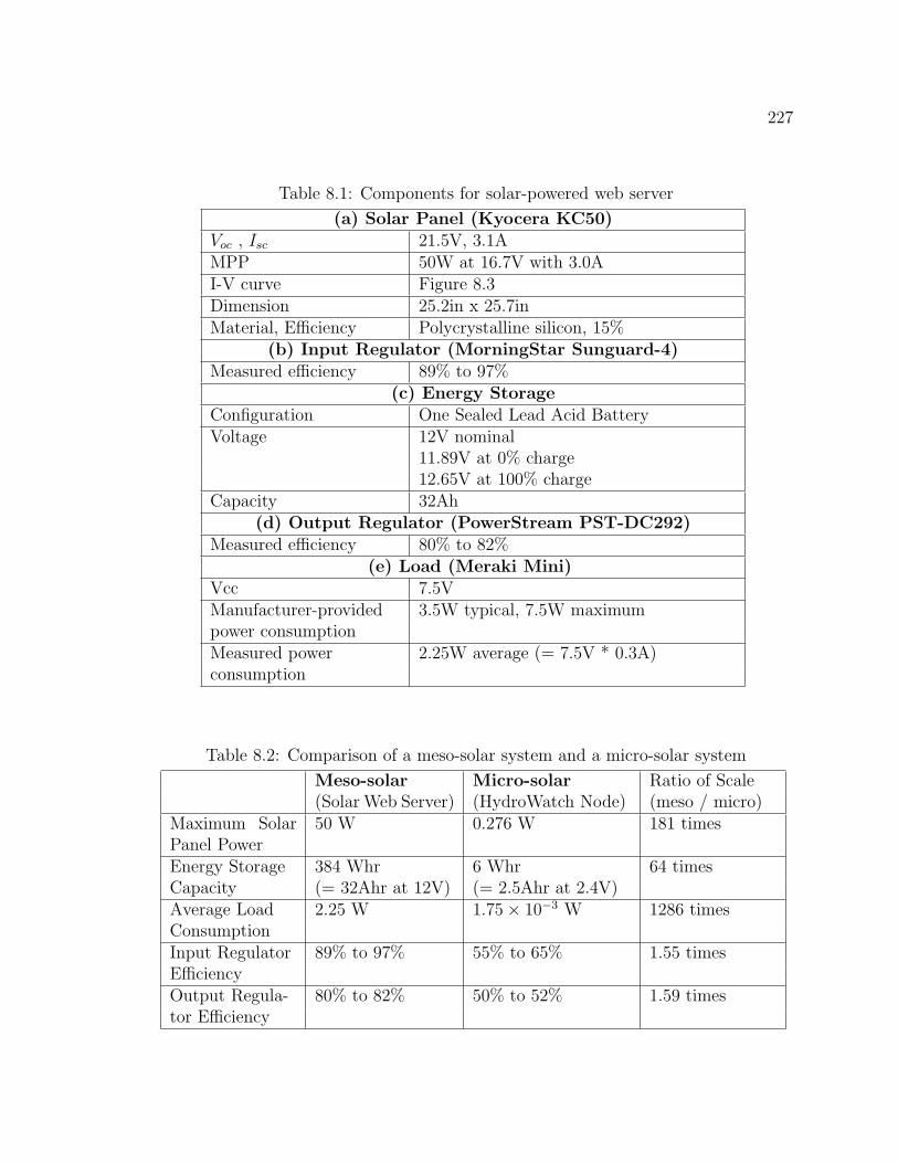
227

Table 8.1: Components for solar-powered web server

(a) Solar Panel (Kyocera KC50)Voc , Isc 21.5V, 3.1AMPP 50W at 16.7V with 3.0AI-V curve Figure 8.3Dimension 25.2in x 25.7inMaterial, Efficiency Polycrystalline silicon, 15%

(b) Input Regulator (MorningStar Sunguard-4)Measured efficiency 89% to 97%

(c) Energy StorageConfiguration One Sealed Lead Acid BatteryVoltage 12V nominal

11.89V at 0% charge12.65V at 100% charge

Capacity 32Ah(d) Output Regulator (PowerStream PST-DC292)

Measured efficiency 80% to 82%(e) Load (Meraki Mini)

Vcc 7.5VManufacturer-provided 3.5W typical, 7.5W maximumpower consumptionMeasured power 2.25W average (= 7.5V * 0.3A)consumption

Table 8.2: Comparison of a meso-solar system and a micro-solar system

Meso-solar Micro-solar Ratio of Scale(Solar Web Server) (HydroWatch Node) (meso / micro)

Maximum SolarPanel Power

50 W 0.276 W 181 times

Energy Storage 384 Whr 6 Whr 64 timesCapacity (= 32Ahr at 12V) (= 2.5Ahr at 2.4V)Average Load 2.25 W 1.75× 10−3 W 1286 timesConsumptionInput Regulator 89% to 97% 55% to 65% 1.55 timesEfficiencyOutput Regula- 80% to 82% 50% to 52% 1.59 timestor Efficiency

228

8.2 Simulating Meso-Solar System

In this subsection, we simulate the behavior of the solar web server under a daily

solar radiation. By comparing the daily energy accumulation and consumption, we

can evaluate whether the meso-solar system can achieve sustainable operation.

8.2.1 Simulation Set-up

For the simulation, the following parameters are considered:

• External Environment: We simulate the meso-solar system that is deployed

on the rooftop of the Computer Science building at UC Berkeley. For this

situation, we can consider the astronomical model with L = 37.87, φp = 180,

τ = 0.1. We simulate the system varying two parameters: solar panel inclination

θp and day of the year n.

– θp: 0 (flat) and 45 (tilted 45◦)

– n: 80 (spring – average case of yearly variation), 356 (winter – worst case

of yearly variation)

• Solar Panel: A Kyocera KC50 50W solar panel is used. The IV-curve in

Figure 8.3 is used to simulate this solar panel.

• Input Regulator: A MorningStar Sunguard-4 12V lead acid battery charging

controller is used. We model the input regulator as a device with 90% efficiency.

The operating points of the input regulator is modeled after the VF -to-IF rela-

tion in Figure 8.5(b).

• Energy Storage: A 12V-32Ah sealed lead acid battery. We estimate the

voltage of the battery based on the charging status (charging or discharging)

and the charge level of the battery. Figure 8.4 describes the charge-to-voltage

relationship for the charging and discharging states.

• Output Regulator: We model the PowerStream PST-DC292 DC-DC con-

verter as a device that has 80% efficiency and 7.77V of output voltage.

229

• Load: A Meraki Mini node is used with a steady state power consumption of

2.25W.

8.2.2 Simulation Result

In simulating the meso-solar system, we are to answer the following two questions:

• Q1 : How much energy can the meso-solar system accumulate, and how does

this affect the sustainability?

• Q2 : How long should the charging period be in order for the system to accu-

mulate the same amount of energy discharged during the night?

In order to answer Q1, we set the initial condition of the simulation so that the

battery does not get full during the day. That way, we can find the daily energy

accumulation without being affected by the battery saturation. In order to answer

Q2, we set the initial condition of the simulation so that the final battery energy level

is the same as the initial level.

Spring

Figure 8.7 shows the simulation result of the daily energy charge and discharge

with the solar-powered web server during spring (n = 80). Whether the solar panel is

flat (Case 1) or tilted (Case 2), the system accumulates more energy than it consumes.

We define the metric battery days as the ratio of battery capacity increase over battery

discharge, and this metric implies how many days the system can operate without

its energy level decreasing. The system has battery days of either 2.1 (Case 1) or 3.0

(Case 2) depending on panel inclination.

Figure 8.8 shows the simulation result of the daily charging and discharging time

with the solar-powered web server during spring (n = 80). Depending on the panel

inclination, the system requires either 4hr 15min (Case 1) or 3hr 45min (Case 2) to

fully charge the battery after darkness on the previous day.

230

0 5 10 15 20 25−20

0

20

40

Time of Day (Hour)

Pow

er (

W)


p = 180, τ = 0.1

0 5 10 15 20 2520

25

30

35

Time of Day (Hour)

Bat

tery

Cap

acity

(A

h)

Ebat_init

= 24Ah, Ebat_final

= 30.1054Ah, Ebat_max

= 32Ah

0 5 10 15 20 25

0

0.5

1

Time of Day (Hour)

0 to

1


= 0.3A

0 5 10 15 20 2512.5

13

13.5

14

14.5

Time of Day (Hour)

Bat

Vol

(V

)

Vbat_init


= 12.656V


Battery Capacity

Load status

Battery Voltage

(a) Case 1: n = 80, θp = 0

0 5 10 15 20 25−20

0

20

40

Time of Day (Hour)

Pow

er (

W)


p = 180, τ = 0.1


0 5 10 15 20 2515

20

25

30

35

Time of Day (Hour)

Bat

tery

Cap

acity

(A

h)

Ebat_init

= 21Ah, Ebat_final


= 32Ah

Battery Capacity

0 5 10 15 20 25

0

0.5

1

Time of Day (Hour)

0 to

1


= 0.3A

Load status

0 5 10 15 20 2512.5

13

13.5

14

Time of Day (Hour)

Bat

Vol

(V

)

Vbat_init


= 12.656V

Battery Voltage

(b) Case 2: n = 80, θp = 45Energy Energy BatteryCharged Discharged Days

Case 1: panel flat 9.1 Ah 3.0 Ah 2.1 daysCase 2: panel tilted 45◦ 11.8 Ah 3.0 Ah 3.0 days

Figure 8.7: Daily energy profile for the solar-powered web server with n = 80. Thebattery is not saturated during the operation.

231

0 5 10 15 20 25−20

0

20

40

Time of Day (Hour)

Pow

er (

W)


p = 180, τ = 0.1


0 5 10 15 20 2529

30

31

32

Time of Day (Hour)

Bat

tery

Cap

acity

(A

h)

Ebat_init

= 30.54Ah, Ebat_final

= 30.54Ah, Ebat_max

= 32Ah

Battery Capacity

0 5 10 15 20 25

0

0.5

1

Time of Day (Hour)

0 to

1


= 0.3A

Load status

0 5 10 15 20 2512.5

13

13.5

14

14.5

Time of Day (Hour)

Bat

Vol

(V

)

Vbat_init


= 12.656V

Battery Voltage

(a) Case 1: n = 80, θp = 0

0 5 10 15 20 25−20

0

20

40

60

Time of Day (Hour)

Pow

er (

W)


p = 180, τ = 0.1


0 5 10 15 20 2529

30

31

32

Time of Day (Hour)

Bat

tery

Cap

acity

(A

h)

Ebat_init



= 32Ah

Battery Capacity

0 5 10 15 20 25

0

0.5

1

Time of Day (Hour)

0 to

1


= 0.3A

Load status

0 5 10 15 20 2512.5

13

13.5

14

14.5

Time of Day (Hour)

Bat

Vol

(V

)

Vbat_init


= 12.656V

Battery Voltage

(b) Case 2: n = 80, θp = 45Energy Energy Charging Discharging

Charged Discharged Time TimeCase 1: panel flat 3.0 Ah 3.0 Ah 4hr 15min 13hr 15minCase 2: panel tilted 45◦ 3.0 Ah 3.0 Ah 3hr 45min 13hr 15min

Figure 8.8: Daily energy profile for the solar-powered web server with n = 80. Thebattery is saturated in middle of day and the final battery level is as the same as theinitial level.

232

Winter

Figure 8.9 shows the simulation result of the daily energy charge and discharge

with the solar-powered web server during winter (n = 356). The system accumulates

more energy than it consumes when the solar panel is tilted (Case 2), and it consumes

more energy when the solar panel is flat (Case 1). For Case 2, the system has 1.6

battery days.

Figure 8.10 shows the simulation result of the daily charging and discharging

time with the solar-powered web server during winter (n = 356). When the panel is

tilted, the system requires 3hr 45min to fully charge the battery after darkness on the

previous day. We consider the case where the panel is tilted because the flat panel

does not provide sufficient energy for sustainable operation.

8.3 Refining the Simulation of a Meso-Solar Sys-

tem Using Measurement Data

Figure 8.11 shows the layout of the solar-powered web server deployment. It

is located on the north-side of the balcony on the UC Berkeley Computer Science

building with its solar panel tilted 45◦ facing south. Thus, the solar panel is obstructed

by the building during the day.

We estimated the daily trend of the solar panel output of the solar-powered web

server using three models: (a) the astronomical model, (b) scaled astronomical model

and (c) obstructed astronomical model. The estimations and the measurement are

shown in Figure 8.12. The measurement result, which is closely captured by the

obstructed astronomical model, is about 44% of the astronomical model estimation.

8.4 Predicting the Behavior of Meso-Solar Sys-

tems

In order to see the long-term behavior of the solar-powered web server, we simu-

lated the meso-solar system with the following parameters:

233

0 5 10 15 20 25−10

0

10

20

Time of Day (Hour)

Pow

er (

W)


p = 180, τ = 0.1


0 5 10 15 20 2522

23

24

25

26

Time of Day (Hour)

Bat

tery

Cap

acity

(A

h)

Ebat_init

= 24Ah, Ebat_final


= 32Ah

Battery Capacity

0 5 10 15 20 25

0

0.5

1

Time of Day (Hour)

0 to

1


= 0.3A

Load status

0 5 10 15 20 2512.5

13

13.5

Time of Day (Hour)

Bat

Vol

(V

)

Vbat_init


= 12.621V

Battery Voltage

(a) Case 1: n = 356, θp = 0

0 5 10 15 20 25−20

0

20

40

Time of Day (Hour)

Pow

er (

W)


p = 180, τ = 0.1


0 5 10 15 20 2520

25

30

35

Time of Day (Hour)

Bat

tery

Cap

acity

(A

h)

Ebat_init

= 24Ah, Ebat_final


= 32Ah

Battery Capacity

0 5 10 15 20 25

0

0.5

1

Time of Day (Hour)

0 to

1


= 0.3A

Load status

0 5 10 15 20 2512.5

13

13.5

14

Time of Day (Hour)

Bat

Vol

(V

)

Vbat_init


= 12.656V

Battery Voltage

(b) Case 2: n = 356, θp = 45Energy Energy BatteryCharged Discharged Days

Case 1: panel flat 3.4 Ah 3.6 Ah -0.1 daysCase 2: panel tilted 45◦ 9.2 Ah 3.5 Ah 1.6 days

Figure 8.9: Daily energy profile for the solar-powered web server with n = 356. Thebattery is not saturated during the operation.

234

0 5 10 15 20 25−20

0

20

40

Time of Day (Hour)

Pow

er (

W)


p = 180, τ = 0.1


0 5 10 15 20 2528

29

30

31

32

Time of Day (Hour)

Bat

tery

Cap

acity

(A

h)

Ebat_init



= 32Ah

Battery Capacity

0 5 10 15 20 25

0

0.5

1

Time of Day (Hour)

0 to

1


= 0.3A

Load status

0 5 10 15 20 2512.5

13

13.5

14

14.5

Time of Day (Hour)

Bat

Vol

(V

)

Vbat_init


= 12.656V

Battery Voltage

Energy Energy Charging DischargingCharged Discharged Time Time

Panel tilted 45◦ 3.5 Ah 3.5 Ah 3hr 45min 15hr 15min

Figure 8.10: Daily energy profile for the solar-powered web server with n = 356,θp = 45. The battery is saturated in middle of day and the final battery level is asthe same as the initial level.

3F

4F

5F

6F

7F

Solar Web Server

Solar Web Server

N N S

Figure 8.11: Layout of the solar-powered web server deployment

235

−5 0 5 10 15 20 250

0.5

1

1.5

2

2.5

3

Time of Day (Hour)

Cur

rent

(A

)

Solar Web Server − Daily Trend with n = 128, θp = 45, L = 37.87, φ

p = 180, τ = 0.1

AstronomicalScaled AstronomicalObstructed AstronomicalMeasured − 5/8/08

Astronomical Scaled Obstructed MeasurementModel Astronomical Astronomical

Daily Radiation 219.65 Wh 161.88 Wh 96.46 Wh 98.04 Wh

Figure 8.12: Estimation of daily solar panel output for the solar-powered web server(n = 128, θp = 45, L = 37.87, φp = 180)

236

• Panel Parameters: panel inclination θp = 45, panel orientation φp = 180

(south), latitude L = 37.87.

• Load Consumption: The effective daily load consumption seen by the solar

panel is Pload ·24h/(Effreg−in ·Effbat ·Effreg−out). For the solar-powered web server,

it is 107.1Wh (= 87.3Wh / (0.9 * 0.8 * 0.7)).

• Time: From 5/8/2008 (n = 128) to 5/8/2009 (n = 365 + 128).

• Estimation Models: Astronomical model, scaled astronomical model and

obstructed astronomical model.

• Comparisons: Daily solar panel output energy and daily battery capacity.

Figure 8.13(a) shows the solar energy estimations and load consumption. While

the daily solar energy for the astronomical model and the scaled astronomical model

is always above the load consumption, the obstructed astronomical model has its

daily solar energy below the load consumption during winter. Thus, the battery level

will drop during winter.

Figure 8.13(b) shows the daily battery level at the end of each day. As we expected,

the battery level stays almost full throughout the year for the astronomical and scaled

astronomical model. For the obstructed astronomical model, the battery level stays

near full capacity during spring, summer and fall. The battery level drops down to

half of the total capacity in the middle of winter and it increases afterwards. This

simulation result assumes clear weather, as depending on the weather conditions

during winter, this system may consume more energy than its battery capacity and

not survive during that time.

237

04/01/08 07/01/08 10/01/08 01/01/09 04/01/09 07/01/090

50

100

150

200

250

300

Date

Dai

ly S

olar

Pan

el E

nerg

y (W

h)

Solar Web Server − Yearly Trend with n = 128, θp = 45, L = 37.87, φ

p = 180, τ = 0.1

AstronomicalScaled AstronomicalObstructed AstronomicalLoad divided by system efficiency

04/01/08 07/01/08 10/01/08 01/01/09 04/01/09 07/01/090

5

10

15

20

25

30

35

Date

Dai

ly F

inal

Bat

tery

Cap

acity

(A

h)

Solar Web Server − Yearly Trend with n = 128, θp = 45, L = 37.87, φ

p = 180, τ = 0.1

AstronomicalScaled AstronomicalObstructed Astronomical

Figure 8.13: Yearly estimation for the solar-powered web server: (a) daily solar paneloutput, (b) daily battery capacity

238

Chapter 9

Concluding Remarks

In this dissertation, we have presented a practical theory that enables a systematic

design of a micro-solar power system. We summarize this dissertation as follows:

First, we developed a general model of micro-solar power systems. While the

design space of micro-solar power systems is very large, it is essential we use the

same simulation framework to represent such diversity in a scalable fashion. We pre-

sented a general model of micro-solar power systems that consisted of several lumped

elements, such as the external environment, a solar collector, an input regulator, en-

ergy storage, output regulator and a load, and their relationship in terms of energy

flow and efficiency factors. In this framework, designing a micro-solar power system

implies setting the parameters of one or more of these lumped elements.

Second, we materialized this model into a simulation suite by formulating each

component of a micro-solar power system as an analytical module and composing

these modules into an instance of a micro-solar power system. To represent a micro-

solar power system in the simulation framework, its components need to be formu-

lated. Depending on the availability and the characteristics of its behavior, each

component is formulated either with an analytical formula, curve fitting, or piecewise

interpolation. To represent the external environment, we proposed three methods: an

astronomical model, an obstructed-astronomical model and a weather-metric model.

The astronomical model estimates solar radiation using well-known formulas without

any knowledge of the deployment site. This model works well on a clear day and

can be used without knowledge of the deployment site, but its estimation error can

239

be high on an overcast day. The obstructed-astronomical model refines the estimates

of the astronomical model by using a few samples of local measurements incurring a

modest estimation error. The weather-metric model further refines the obstructed-

astronomical model by adjusting the solar radiation by the amount of weather effects.

Using all of these components, we have composed a few instances of micro-solar power

systems. Using benchtop experiments, we have shown that this simulation tools work

in a small time frame.

Third, we have implemented a reference platform of a micro-solar power system,

the HydroWatch node, and validated the simulation suite by comparing solar energy

estimates with empirical results in a realistic environment. The short-term deploy-

ment, where reference platform nodes were placed under varying solar profiles in

urban neighborhoods and forest watershed environments, showed that our simula-

tion tools could estimate the solar energy budget with only a small degree of error.

The long-term deployment, where reference platform nodes were placed on an urban

rooftop environment, showed that our simulation tools could estimate the solar en-

ergy budget of a system under varying weather conditions and that the difference

between estimates and empirical results was bounded by roughly 30%. We reduced

this estimation error even further with a weather metric model, predicting the solar

radiation with a 6% margin of error by maintaining a week of cloud condition history.

Finally, we extended the simulation suite for hypothetical designs of micro-solar

power systems and meso-solar power systems, demonstrating that our model and sim-

ulation suite can be used beyond the reference design of micro-solar power systems.

As an example of a hypothetical design, we simulated a micro-solar power system with

multi-level energy storage consisting of a supercapacitor and NiMH batteries. This al-

lowed us to find how parameters of a hypothetical system affect system performance.

Next, we extended the simulator for wind and vibration energy. Our preliminary

study shows that the simulator can be adapted for other renewable energy sources

in a straightforward way by modeling the external environment and energy collec-

tor components. Lastly, as a meso-solar system, we designed a solar-powered web

server by composing Watt-scale components and simulated this design by modeling

each component and integrating it into the simulator. The measurements from the

implementation validated our model with a solar power system of a larger scale.

240

Bibliography

[Arc] Arch Rock Corporation. Arch Rock Corporation, Primer Pack / IP. http:

//www.archrock.com/downloads/datasheet/primerpack datasheet.pdf.

[BMS] Solar Radiation Research Laboratory. http://www.nrel.gov/midc/srrl

bms/.

[Cal] California Solar Initiative. Incentive Calculator. http://www.csi-epbb.

com.

[CH88] Theodore W. Cannon and Roland L. Hulstrom. The atmospheric op-

tical calibration system. The Twentieth IEEE Photovoltaic Specialists

Conference, September 1988.

[CJBM01] Benjie Chen, Kyle Jamieson, Hari Balakrishnan, and Robert Morris.

Span: an energy-efficient coordination algorithm for topology mainte-

nance in ad hoc wireless networks. The Seventh Annual International

Conference on Mobile Computing and Networking (MobiCom ‘01), July

2001.

[COSKM05] Rachel Cardell-Oliver, Keith Smettem, Mark Kranz, and Kevin Mayer.

A reactive soil moisture sensor network: Design and field evaluation. In-

ternational Journal of Distributed Sensor Networks (IJDSN ‘05), March

2005.

[CVS+07] Peter Corke, Philip Valencia, Pavan Sikka, Tim Wark, and Les Overs.

Long-duration solar-powered wireless sensor networks. The Fourth IEEE

workshop on Embedded Networked Sensors (EmNets ‘07), June 2007.

http://www.archrock.com/downloads/datasheet/primerpack_datasheet.pdf

http://www.archrock.com/downloads/datasheet/primerpack_datasheet.pdf

http://www.nrel.gov/midc/srrl_bms/

http://www.nrel.gov/midc/srrl_bms/

http://www.csi-epbb.com

http://www.csi-epbb.com

241

[DHJ+06] Prabal Dutta, Jonathan Hui, Jaein Jeong, Sukun Kim, Cory Sharp, Jay

Taneja, Gilman Tolle, Kamin Whitehouse, and David Culler. Trio: En-

abling sustainable and scalable outdoor wireless sensor network deploy-

ments. The Fifth International Conference on Information Processing

in Sensor Networks (IPSN/SPOTS ‘06), April 2006.

[DHM75] J. V. Dave, P. Halpern, and H. J. Myers. Computation of incident solar

energy. IBM Journal of Research and Development, 19(6):539–549, 1975.

[Dus] Dust Networks. Technical Overview of Time Synchronized Mesh Proto-

col (TSMP). http://www.dustnetworks.com/docs/TSMP Whitepaper.

pdf.

[EV06] Sinem Coleri Ergen and Pravin Varaiya. Pedamacs: Power efficient and

delay aware medium access protocol for sensor networks. IEEE Trans-

actions on Mobile Computing, 5(7), July 2006.

[fin] FindSolar: Connecting You to Renewable Energy Professionals. http:

//findsolar.com.

[GCD+98] Vahan Gevorgian, David A. Corbus, Stephen Drouilhet, Richard Holz,

and Karen E. Thomas. Modeling, testing and economic analysis of a

wind-electric battery charging station. Windpower ‘98, 1998.

[Har] Harvard University. MoteLab. http://motelab.eecs.harvard.edu/.

[HKWW06] Vlado Handziski, Andreas Kopke, Andreas Willig, and Adam Wolisz.

Twist: a scalable and reconfigurable testbed for wireless indoor experi-

ments with sensor networks. The 2nd international workshop on Multi-

hop ad hoc networks: from theory to reality (REALMAN ‘06), 2006.

[HZKS06] Jason Hsu, Sadaf Zahedi, Aman Kansal, and Mani B Srivastava. Adap-

tive duty cycling for energy harvesting systems. International Symposium

on Low Power Electronics and Design (ISLPED ‘06), 2006.

[Int] Intel Research, Berkeley. Mirage: Microeconomic resource allocation for

sensornet testbeds. http://mirage.berkeley.intel-research.net.

http://www.dustnetworks.com/docs/TSMP_Whitepaper.pdf

http://www.dustnetworks.com/docs/TSMP_Whitepaper.pdf

http://findsolar.com

http://findsolar.com

http://motelab.eecs.harvard.edu/

http://mirage.berkeley.intel-research.net

242

[Iow] Iowa Energy Center. Solar Data for Iowa Locations. http://www.energy.

iastate.edu/renewable/solar/calculator.

[JPC05] Xiaofan Jiang, Joseph Polastre, and David Culler. Perpetual environ-

mentally powered sensor networks. The Fourth International Sympo-

sium on Information Processing in Sensor Networks (IPSN/SPOTS ‘05),

April 2005.

[KHZS07] Aman Kansal, Jason Hsu, Sadaf Zahedi, and Mani B. Srivastava. Power

management in energy harvesting sensor networks. ACM Transactions

in Embedded Computing Systems, 2007.

[Kim07] Sukun Kim. Wireless sensor networks for high frequency sampling. Ph.D

Thesis, University of California at Berkeley, December 2007.

[KPS04] Aman Kansal, Dunny Potter, and Mani B. Srivastava. Performance

aware tasking for environmentally powered sensor networks. The joint

international conference on Measurement and modeling of computer sys-

tems (ACM SIGMETRICS ‘04), June 2004.

[Kyo] Kyocera. KC50 High Efficiency Multicrystal Photovoltaic Module.

http://www.wholesalesolar.com/pdf.folder/module%20pdf%20folder/

KC50.pdf.

[LBV06] Koen Langendoen, Aline Baggio, and Otto Visser. Murphy loves pota-

toes: Experiences from a pilot sensor network deployment in precision

agriculture. Workshop on Parallel and Distributed Real-Time Systems

(WPDRTS ‘06), April 2006.

[LLWC03] Philip Levis, Nelson Lee, Matt Welsh, and David Culler. Tossim: Ac-

curate and scalable simulation of entire tinyos applications. The First

ACM Conference on Embedded Networked Sensor Systems (Sensys ‘03),

2003.

[LPCS04] P. Levis, N. Patel, D. Culler, and S. Shenker. Trickle: A self-regulating

algorithm for code propagation and maintenance in wireless sensor net-

http://www.energy.iastate.edu/renewable/solar/calculator

http://www.energy.iastate.edu/renewable/solar/calculator

http://www.wholesalesolar.com/pdf.folder/module%20pdf%20folder/KC50.pdf

http://www.wholesalesolar.com/pdf.folder/module%20pdf%20folder/KC50.pdf

243

works. The First Symposium on Networked Systems Design and Imple-

mentation (NSDI ‘04), March 2004.

[LWG05] Olaf Landsiedel, Klaus Wehrle, and Stefan Gotz. Accurate prediction of

power consumption in sensor networks. The Second IEEE workshop on

Embedded Networked Sensors (EmNets ‘05), 2005.

[MBTB06a] C. Moser, B. Brunelli, L. Thiele, and L. Benini. Lazy scheduling for

energy harvesting sensor nodes. IFIP Model-Driven Design to Resource

Management for Distributed Embedded Systems, 2006.

[MBTB06b] C. Moser, B. Brunelli, L. Thiele, and L. Benini. Real-time scheduling

with regenerative energy. The 18th Euromicro Conference on Real-Time

Systems (ECRTS ‘06), 2006.

[Mer] Meraki. Meraki Mini. http://meraki.com/oursolution/hardware/mini/.

[Met] Meteonorm. Meteonorm. http://www.meteotest.ch/pdf/am/mn

description.pdf.

[MFHH02] Samuel Madden, Michael J. Franklin, Joseph M. Hellerstein, and Wei

Hong. Tag: a tiny aggregation service for ad-hoc sensor networks. The

fifth symposium on Operating systems design and implementation (OSDI

‘02), December 2002.

[MKHC07] G. Montenegro, N. Kushalnagar, J. Hui, and D. Culler. Transmission of

ipv6 packets over ieee 802.15.4 networks, September 2007. http://tools.

ietf.org/html/rfc4944.

[Nat] National Renewable Energy Laboratory. PVWATTS: A Performance

Calculator for Grid-Connected PV Systems. http://rredc.nrel.gov/solar/

codes algs/PVWATTS.

[New78] Arthur Richard Newton. The simulation of large scale integrated circuits.

Ph.D Thesis, University of California at Berkeley, Dec 1978.

http://meraki.com/oursolution/hardware/mini/

http://www.meteotest.ch/pdf/am/mn_description.pdf

http://www.meteotest.ch/pdf/am/mn_description.pdf

http://tools.ietf.org/html/rfc4944

http://tools.ietf.org/html/rfc4944

http://rredc.nrel.gov/solar/codes_algs/PVWATTS

http://rredc.nrel.gov/solar/codes_algs/PVWATTS

244

[NGSA04] Suman Nath, Phillip B. Gibbons, Srinivasan Seshan, and Zachary R.

Anderson. Synopsis diffusion for robust aggregation in sensor networks.

The Second ACM Conference on Embedded Networked Sensor Systems

(Sensys ‘04), November 2004.

[NLA+07] Ani Nahapetian, Paolo Lombardo, Andrea Acquaviva, Luca Benini, and

Majid Sarrafzadeh. Dynamic reconfiguration in sensor networks with

regenerative energy sources. The conference on Design, automation and

test in Europe (EDAA ‘07), 2007.

[NSR] National Solar Radiation Data Base. ftp://ftp3.ncdc.noaa.gov/pub/

data/nsrdb.

[Par06] Joseph A. Paradiso. Systems for human-powered mobile computing.

IEEE Design Automation Conference (DAC ‘06), 2006.

[PC06] Chulsung Park and Pai H. Chou. Ambimax: Autonomous energy har-

vesting platform for multi-supply wireless sensor nodes. IEEE Sensor

and Ad Hoc Communications and Networks (SECON ‘06), 2006.

[Per93] Richard Perez. Lead-acid battery state of charge vs. voltage. Home

Power, 36, Aug/Sep 1993. http://www.arttec.net/Solar Mower/4

Electrical/Battery%20Charging.pdf.

[PFR78] James T. Peterson, Edwin C. Flowers, and John H. Rudisill. Urban-rural

solar radiation and atmospheric turbidity measurements in the los ange-

les basin. Journal of Applied Meteorology, 17(11):1595–1609, November

1978.

[PHC04] Joseph Polastre, Jason Hill, and David Culler. Versatile low power media

access for wireless sensor networks. The Second ACM Conference on

Embedded Networked Sensor Systems (Sensys ‘04), November 2004.

[PKR02] S. Sandeep Pradhan, Julius Kusuma, and Kannan Ramchandran. Dis-

tributed compression in a dense microsensor network. IEEE Signal Pro-

cessing Magazine, March 2002.

ftp://ftp3.ncdc.noaa.gov/pub/data/nsrdb

ftp://ftp3.ncdc.noaa.gov/pub/data/nsrdb

http://www.arttec.net/Solar_Mower/4_Electrical/Battery%20Charging.pdf

http://www.arttec.net/Solar_Mower/4_Electrical/Battery%20Charging.pdf

245

[Pow] PowerStream. PST-DC292. http://www.powerstream.com/dc6.htm.

[PSC05] Joseph Polastre, Robert Szewczyk, and David Culler. Telos: Enabling

ultra-low power wireless research. The Fourth International Sympo-

sium on Information Processing in Sensor Networks (IPSN/SPOTS ‘05),

April 2005.

[PSS00] Sung Park, Andreas Savvides, and Mani B. Srivastava. Sensorsim:

A simulation framework for sensor networks. International Workshop

on Modeling Analysis and Simulation of Wireless and Mobile Systems

(MSWIM ‘00), 2000.

[PSS01] Sung Park, Andreas Savvides, and Mani B. Srivastava. Simulating net-

works of wireless sensors. Winter Simulation Conference, 2001.

[RKH+05] Vijay Raghunathan, Aman Kansal, Jason Hsu, Jonathan Friedman, and

Mani Srivastava. Design considerations for solar energy harvesting wire-

less embedded systems. The Fourth International Symposium on Infor-

mation Processing in Sensor Networks (IPSN/SPOTS ‘05), April 2005.

[ROC+03] Shad Roundy, Brian P. Otis, Yuen-Hui Chee, Jan M. Rabaey, and Paul

Wright. A 1.9ghz rf transmit beacon using environmentally scavenged

energy. International Symposium on Low Power Electronics and Design

(ISLPED ‘03), Aug. 2003.

[Rou03] Shad J. Roundy. Energy scavenging for wireless sensor nodes with a

focus on vibration to electricity conversion. Ph.D Thesis, University of

California at Berkeley, May 2003.

[RSF+04] Shad Roundy, Dan Steingart, Luc Frechette, Paul Wright, and Jan

Rabaey. Power sources for wireless sensor networks. The First European

Workshop on Wireless Sensor Networks (EWSN ‘04), January 2004.

[RV82] Elmer Robinson and Ralph J. Valente. Atmospheric turbidity over the

united states from 1967 to 1976. U.S. Environmental Protection Agency

Report 600382076, September 1982.

http://www.powerstream.com/dc6.htm

246

[SC06] Farhan Simjee and Pai H. Chou. Everlast: Long-life, supercapacitor-

operated wireless sensor node. International Symposium on Low Power

Electronics and Design (ISLPED ‘06), October 2006.

[SCV+06] Pavan Sikka, Peter Corke, Philip Valencia, Christopher Crossman, Dave

Swain, and Greg Bishop-Hurley. Wireless adhoc sensor and actuator net-

works on the farm. The Fifth International Conference on Information

Processing in Sensor Networks (IPSN/SPOTS ‘06), 2006.

[Sen] Sentilla. Sentilla Tmote Sky. http://www.sentilla.com/pdf/eol/

tmote-sky-datasheet.pdf.

[SHC+04] Victor Shnayder, Mark Hempstead, Borrong Chen, Geoff Werner-Allen,

and Matt Welsh. Simulating the power consumption of large-scale sen-

sor network applications. The Second ACM Conference on Embedded

Networked Sensor Systems (Sensys ‘04), November 2004.

[SKA04] Sameer Sundresh, Wooyoung Kim, and Gul Agha. Sens: a sensor, en-

vironment and network simulator. The 37th Annual Simulation Sympo-

sium (ANSS ‘04), 2004.

[SKG+07] Jacob Sober, Alexander Kostadinov, Matthew Garber, Matthew Bren-

nan, Mark D. Corner, and Emergy D. Berger. Eon: A language and

runtime system for perpetual systems. The Fifth ACM Conference on

Embedded Networked Sensor Systems (Sensys ‘07), 2007.

[SMP+04] Robert Szewczyk, Alan Mainwaring, Joseph Polastre, John Anderson,

and David Culler. An analysis of a large scale habitat monitoring ap-

plication. The Second ACM Conference on Embedded Networked Sensor

Systems (Sensys ‘04), November 2004.

[SOP+04] Robert Szewczyk, Eric Osterweil, Joseph Polastre, Michael Hamilton,

Alan Mainwaring, and Deborah Estrin. Habitat monitoring with sensor

networks. Communications of the ACM, 47(6):34–40, 2004.

http://www.sentilla.com/pdf/eol/tmote-sky-datasheet.pdf

http://www.sentilla.com/pdf/eol/tmote-sky-datasheet.pdf

247

[SS02] Anna Scaglione and Sergio Servetto. On the interdependence of routing

and data compression in multi-hop sensor networks. The 8th Annual In-

ternational Conference on Mobile Computing and Networking (MobiCom

‘02), 2002.

[Sun] Sunpower. Supower Solar Calculator. http://www.sunpowercorp.com/

For-Homes/How-To-Buy/Solar-Calculator.aspx.

[SVML03] Gyula Simon, Peter Volgyesi, Miklos Maroti, and Akos Ledeczi.

Simulation-based optimization of communication protocols for large-

scale wireless sensor networks. IEEE Aerospace Conference, 2003.

[Tec] Linear Technology. LTC1751: Micropower, Regulated Charge Pump

DC/DC Converter. http://www.linear.com/pc/downloadDocument.do?

navId=H0,C1,C1003,C1039,C1133,P1904,D2062.

[TJC08] Jay Taneja, Jaein Jeong, and David Culler. Design, modeling, and ca-

pacity planning for micro-solar power sensor networks. The Seventh

International Conference on Information Processing in Sensor Networks

(IPSN/SPOTS ‘08), April 2008.

[TLP05] Ben L. Titzer, Daniel K. Lee, and Jens Palsberg. Avrora: scalable sen-

sor network simulation with precise timing. The Fourth International

Symposium on Information Processing in Sensor Networks (IPSN ‘05),

2005.

[TPS+05] Gilman Tolle, Joseph Polastre, Robert Szewczyk, David Culler, Neil

Turner, Kevin Tu, Stephen Burgess, Todd Dawson, Phil Buonadonna,

David Gay, and Wei Hong. A macroscope in the redwoods. The Third


November 2005.

[Unia] University of California, Berkeley. HydroWatch Project. http://

hydrowatch.cs.berkeley.edu.

[Unib] University of California, Berkeley. Smote Testbed. http://smote.cs.

berkeley.edu.

http://www.sunpowercorp.com/For-Homes/How-To-Buy/Solar-Calculator.aspx

http://www.sunpowercorp.com/For-Homes/How-To-Buy/Solar-Calculator.aspx

http://www.linear.com/pc/downloadDocument.do?navId=H0,C1,C1003,C1039,C1133,P1904,D2062

http://www.linear.com/pc/downloadDocument.do?navId=H0,C1,C1003,C1039,C1133,P1904,D2062

http://hydrowatch.cs.berkeley.edu

http://hydrowatch.cs.berkeley.edu

http://smote.cs.berkeley.edu

http://smote.cs.berkeley.edu

248

[vDL03] Tijs van Dam and Koen Langendoen. An adaptive energy-efficient mac

protocol for wireless sensor networks. The First ACM Conference on

Embedded Networked Sensor Systems (Sensys ‘03), November 2003.

[VGB07] Christopher M. Vigorito, Deepak Ganesan, and Andrew G. Barto. Adap-

tive control of duty cycling in energy-harvesting wireless sensor networks.

IEEE Sensor and Ad Hoc Communications and Networks (SECON ‘07),

2007.

[VXSB07] Maneesh Varshney, Defeng Xu, Mani Srivastava, and Rajive Bagrodia.

squalnet: A scalable simulation and emulation environment for sensor

networks. The Seventh International Conference on Information Pro-

cessing in Sensor Networks (IPSN/SPOTS ‘07), 2007.

[WAJR+05] Geoffrey Werner-Allen, Jeff Johnson, Mario Ruiz, Jonathan Lees, and

Matt Welsh. Monitoring volcanic eruptions with a wireless sensor net-

work. The Second European Workshop on Wireless Sensor Networks

(EWSN ‘05), January 2005.

[WASW05] Geoffrey Werner-Allen, Patrick Swieskowski, and Matt Welsh. Mote-

lab: A wireless sensor network testbed. The Fourth International Sym-

posium on Information Processing in Sensor Networks (IPSN/SPOTS

‘05), April 2005.

[Wea] Weather Underground. Solar Calculator. http://www.wunderground.

com/calculators/solar.html.

[Wik] Wikipedia. Lead-acid battery. http://en.wikipedia.org/wiki/Lead acid

battery.

[Wun] Weather Underground. http://www.wunderground.com.

[YHE04] Wei Ye, John Heidemann, and Deborah Estrin. Medium access con-

trol with coordinated adaptive sleeping for wireless sensor networks.

IEEE/ACM Transactions on Networking, 3, June 2004.

http://www.wunderground.com/calculators/solar.html

http://www.wunderground.com/calculators/solar.html

http://en.wikipedia.org/wiki/Lead_acid_battery

http://en.wikipedia.org/wiki/Lead_acid_battery

http://www.wunderground.com

249

[YSH06] Wei Ye, Fabio Silva, and John Heidemann. Ultra-low duty cycle mac with

scheduled channel polling. The Fourth ACM Conference on Embedded

Networked Sensor Systems (Sensys ‘06), November 2006.

[ZSLM04] Pei Zhang, Christopher M. Sadler, Stephen A. Lyon, and Margaret

Martonosi. Hardware design experiences in zebranet. The Second


November 2004.

[ZZH+07] Jingbin Zhang, Gang Zhou, Chengdu Huang, Sang H. Son, and John A.

Stankovic. Tmmac: An energy efficient multi-channel mac protocol for

ad hoc networks. IEEE International Conference on Communications

(ICC ‘07), June 2007.

A Practical Theory of Micro-Solar Power Sensor Networks · A Practical Theory of Micro-Solar Power...

Documents

Transcript of A Practical Theory of Micro-Solar Power Sensor Networks · A Practical Theory of Micro-Solar Power...