A practical Introduction to Machine(s) Learning
77
A practical Introduction to Machine(s) Learning Csvop!Hpo³bmwft www.bgoncalves.com
-
Upload
bruno-goncalves -
Category
Data & Analytics
-
view
930 -
download
0
Transcript of A practical Introduction to Machine(s) Learning

A practical Introduction to Machine(s) Learning
www.bgoncalves.com

www.bgoncalves.com@bgoncalves

www.bgoncalves.com@bgoncalves
Time
CPUData
BigData
Moore’s Law
Big Data
1997

www.bgoncalves.com@bgoncalves
http://static.googleusercontent.com/media/research.google.com/en//pubs/archive/35179.pdf
E X P E R T O P I N I O N
8 1541-1672/09/$25.00 © 2009 IEEE IEEE INTELLIGENT SYSTEMSPublished by the IEEE Computer Society
Contact Editor: Brian Brannon, [email protected]
such as f = ma or e = mc2. Meanwhile, sciences that involve human beings rather than elementary par-ticles have proven more resistant to elegant math-ematics. Economists suffer from physics envy over their inability to neatly model human behavior. An informal, incomplete grammar of the English language runs over 1,700 pages.2 Perhaps when it comes to natural language processing and related fi elds, we’re doomed to complex theories that will never have the elegance of physics equations. But if that’s so, we should stop acting as if our goal is to author extremely elegant theories, and instead embrace complexity and make use of the best ally we have: the unreasonable effectiveness of data.
One of us, as an undergraduate at Brown Univer-sity, remembers the excitement of having access to the Brown Corpus, containing one million English words.3 Since then, our fi eld has seen several notable corpora that are about 100 times larger, and in 2006, Google released a trillion-word corpus with frequency counts for all sequences up to fi ve words long.4 In some ways this corpus is a step backwards from the Brown Corpus: it’s taken from unfi ltered Web pages and thus contains incomplete sentences, spelling er-rors, grammatical errors, and all sorts of other er-rors. It’s not annotated with carefully hand-corrected part-of-speech tags. But the fact that it’s a million times larger than the Brown Corpus outweighs these drawbacks. A trillion-word corpus—along with other Web-derived corpora of millions, billions, or tril-lions of links, videos, images, tables, and user inter-actions—captures even very rare aspects of human
behavior. So, this corpus could serve as the basis of a complete model for certain tasks—if only we knew how to extract the model from the data.
Learning from Text at Web ScaleThe biggest successes in natural-language-related machine learning have been statistical speech rec-ognition and statistical machine translation. The reason for these successes is not that these tasks are easier than other tasks; they are in fact much harder than tasks such as document classifi cation that ex-tract just a few bits of information from each doc-ument. The reason is that translation is a natural task routinely done every day for a real human need (think of the operations of the European Union or of news agencies). The same is true of speech tran-scription (think of closed-caption broadcasts). In other words, a large training set of the input-output behavior that we seek to automate is available to us in the wild. In contrast, traditional natural language processing problems such as document classifi ca-tion, part-of-speech tagging, named-entity recogni-tion, or parsing are not routine tasks, so they have no large corpus available in the wild. Instead, a cor-pus for these tasks requires skilled human annota-tion. Such annotation is not only slow and expen-sive to acquire but also diffi cult for experts to agree on, being bedeviled by many of the diffi culties we discuss later in relation to the Semantic Web. The fi rst lesson of Web-scale learning is to use available large-scale data rather than hoping for annotated data that isn’t available. For instance, we fi nd that useful semantic relationships can be automatically learned from the statistics of search queries and the corresponding results5 or from the accumulated evi-dence of Web-based text patterns and formatted ta-bles,6 in both cases without needing any manually annotated data.
Eugene Wigner’s article “The Unreasonable Ef-
fectiveness of Mathematics in the Natural Sci-
ences”1 examines why so much of physics can be
neatly explained with simple mathematical formulas
Alon Halevy, Peter Norvig, and Fernando Pereira, Google
The Unreasonable Effectiveness of Data
Authorized licensed use limited to: Univ of Calif Berkeley. Downloaded on February 5, 2010 at 22:51 from IEEE Xplore. Restrictions apply.
Big Data

www.bgoncalves.com@bgoncalves
Dataset Size
Mod
el Qu
ality
Big Data

www.bgoncalves.com@bgoncalves
Big Datahttps://www.wired.com/2008/06/pb-theory/

www.bgoncalves.com@bgoncalves
From Data To Information
2 Chapter 1
Statistics are everywhereEverywhere you look you can find statistics, whether you’re browsing the Internet, playing sports, or looking through the top scores of your favorite video game. But what actually is a statistic?
Statistics are numbers that summarize raw facts and figures in some meaningful way. They present key ideas that may not be immediately apparent by just looking at the raw data, and by data, we mean facts or figures from which we can draw conclusions. As an example, you don’t have to wade through lots of football scores when all you want to know is the league position of your favorite team. You need a statistic to quickly give you the information you need.
The study of statistics covers where statistics come from, how to calculate them, and how you can use them effectively.
Gather data
Analyze
Draw conclusionsWhen you’ve analyzed your data, you make decisions and predictions.
Once you have data, you can analyze it and generate statistics. You can calculate probabilities to see how likely certain events are, test ideas, and indicate how confident you are about your results.
At the root of statistics is data.
Data can be gathered by looking
through existing sources, conducting
experiments, or by conducting surveys.
welcome to statsville!

www.bgoncalves.com@bgoncalves
“Zero is the most natural number”(E. W. Dijkstra)
Count!
• How many items do we have?

www.bgoncalves.com@bgoncalves
Descriptive Statistics
Min Max
Mean µ =1
N
NX
i=1
xi
� =
vuut 1
N
NX
i=1
(xi � µ)2StandardDeviation

www.bgoncalves.com@bgoncalves
Anscombe’s Quartetx1 y1
10.0 8.04
8.0 6.95
13.0 7.58
9.0 8.81
11.0 8.33
14.0 9.96
6.0 7.24
4.0 4.26
12.0 10.84
7.0 4.82
5.0 5.68
x2 y2
10.0 9.14
8.0 8.14
13.0 8.74
9.0 8.77
11.0 9.26
14.0 8.10
6.0 6.13
4.0 3.10
12.0 9.13
7.0 7.26
5.0 4.74
x3 y3
10.0 7.46
8.0 6.77
13.0 12.74
9.0 7.11
11.0 7.81
14.0 8.84
6.0 6.08
4.0 5.39
12.0 8.15
7.0 6.42
5.0 5.73
x4 y4
8.0 6.58
8.0 5.76
8.0 7.71
8.0 8.84
8.0 8.47
8.0 7.04
8.0 5.25
19.0 12.50
8.0 5.56
8.0 7.91
8.0 6.89
9
11
7.50
~4.125
0.816
fit y=3+0.5x
µx
µy
�y
�x
⇢
03.256.5
9.7513
0 5 10 15 20
03.256.5
9.7513
0 5 10 15 20
03.256.5
9.7513
0 5 10 15 20
03.256.5
9.7513
0 5 10 15 20

www.bgoncalves.com@bgoncalves
Central Limit Theorem
• As the random variables:
• with:
• converge to a normal distribution:
• after some manipulations, we find:
n ! 1
Sn =1
n
X
i
xi
N�0,�2
�
pn (Sn � µ)
Sn ⇠ µ+N
�0,�2
�pn
The estimation of the mean converges to the true mean with the square root of the number of samples
! SE =�pn

www.bgoncalves.com@bgoncalves
Gaussian Distribution - Maximally Entropic
PN (x, µ,�) =1p2�
e
� (x�µ)2
2�2

www.bgoncalves.com@bgoncalves
Experimental Measurements
• Experimental errors commonly assumed gaussian distributed
• Many experimental measurements are actually averages:
• Instruments have a finite response time and the quantity of interest varies quickly over time
• Stochastic Environmental factors
• Etc

www.bgoncalves.com@bgoncalves
• In an experimental measurement, we expect (CLT) the experimental values to be normally distributed around the theoretical value with a certain variance. Mathematically, this means:
• where are the experimental values and the theoretical ones. The likelihood is then:
• Where we see that to maximize the likelihood we must minimize the sum of squares
MLE - Fitting a theoretical function to experimental data
y � f (x) ⇡ 1p2�
2exp
"� (y � f (x))
2
2�
2
#
yf (x)
Least Squares Fitting
L = �N
2
log
⇥2�
2⇤�
X
i
"(yi � f (xi))
2
2�
2
#

www.bgoncalves.com@bgoncalves
MLE - Linear Regression• Let’s say we want to fit a straight line to a set of points:
• The Likelihood function then becomes:
• With partial derivatives:
• Setting to zero and solving for and :
y = w · x+ b
L = �N
2
log
⇥2�
2⇤�X
i
"(yi � w · xi � b)
2
2�
2
#
@L@w
=X
i
[2xi (yi � w · xi � b)]
@L@b
=X
i
[(yi � w · xi � b)]
w =
Pi (xi � hxi) (yi � hyi)P
i (xi � hxi)2
b = hyi � whxi
w b

@bgoncalves
MLE for Linear Regressionfrom __future__ import print_function import sys import numpy as np from scipy import optimize
data = np.loadtxt(sys.argv[1])
x = data.T[0] y = data.T[1]
meanx = np.mean(x) meany = np.mean(y)
w = np.sum((x-meanx)*(y-meany))/np.sum((x-meanx)**2) b = meany-w*meanx
print(w, b)
#We can also optimize the Likelihood expression directly def likelihood(w): global x, y sigma = 1.0 w, b = w
return np.sum((y-w*x-b)**2)/(2*sigma)
w, b = optimize.fmin_bfgs(likelihood, [1.0, 1.0])
print(w, b)
MLElinear.py

www.bgoncalves.com@bgoncalves
Geometric Interpretation
0
3.25
6.5
9.75
13
0 5 10 15 20
L = �N
2
log
⇥2�
2⇤�
X
i
"(yi � f (xi))
2
2�
2
#
Quadra t i c e r ro r means that an error twice as large is p e n a l i z e d f o u r times as much.

www.bgoncalves.com@bgoncalves
`
0
3.25
6.5
9.75
13
0 5 10 15 20
2D
y = !0 + !1x1
3D
y = !0 + !1x1 + !2x2
Geometric Interpretation
nD
y = ~!
T~x

www.bgoncalves.com@bgoncalves
How do Machines Learn?

www.bgoncalves.com@bgoncalves
3 Types of Machine Learning
• Unsupervised Learning
• Autonomously learn an good representation of the dataset
• Find clusters in input
• Supervised Learning
• Predict output given input
• Training set of known inputs and outputs is provided
• Reinforcement Learning
• Learn sequence of actions to maximize payoff
• Discount factor for delayed rewards

www.bgoncalves.com@bgoncalves
Unsupervised Learning • Extracting patters from data
• K-Means
• PCA

www.bgoncalves.com@bgoncalves
Clustering

www.bgoncalves.com@bgoncalves
K-Means
• Choose k randomly chosen points to be the centroid of each cluster
• Assign each point to belong the cluster whose centroid is closest
• Recompute the centroid positions (mean cluster position)
• Repeat until convergence

www.bgoncalves.com@bgoncalves
K-Means: Structure Voronoi Tesselation

www.bgoncalves.com@bgoncalves
K-Means: Convergence• How to quantify the “quality” of the solution found at each iteration, ?
• Measure the “Inertia”, the square intra-cluster distance:where are the coordinates of the centroid of the cluster to which is assigned.
• Smaller values are better
• Can stop when the relative variation is smaller than some value
µi xi
In+1 � In
In< tol
In =NX
i=0
kxi � µik2
n

@bgoncalves
K-Means: sklearnfrom sklearn.cluster import KMeans
kmeans = KMeans(n_clusters=nclusters) kmeans.fit(data)
centroids = kmeans.cluster_centers_ labels = kmeans.labels_
KMeans.py

www.bgoncalves.com@bgoncalves
K-Means: Limitations

www.bgoncalves.com@bgoncalves
K-Means: Limitations
• No guarantees about Finding “Best” solution
• Each run can find different solution
• No clear way to determine “k”

www.bgoncalves.com@bgoncalves
Silhouettes• For each point define as: the average distance between point and every other point within cluster .
• Let be: the minimum value of excluding
• The silhouette of is then:
ac (xi)
ac (xi) =1
Nc
X
j2c
kxi � xjk
b (xi) = minc 6=ci
ac (xi)
s (xi) =b (xi)� aci (xi)
max {b (xi) , aci (xi)}
xi
xi c
b (xi)
ciac (xi)
xi

www.bgoncalves.com@bgoncalves
Silhouetteshttp://scikit-learn.org/stable/auto_examples/cluster/plot_kmeans_silhouette_analysis.html

www.bgoncalves.com@bgoncalves
Silhouetteshttp://scikit-learn.org/stable/auto_examples/cluster/plot_kmeans_silhouette_analysis.html

www.bgoncalves.com@bgoncalves
Silhouetteshttp://scikit-learn.org/stable/auto_examples/cluster/plot_kmeans_silhouette_analysis.html

www.bgoncalves.com@bgoncalves
Silhouetteshttp://scikit-learn.org/stable/auto_examples/cluster/plot_kmeans_silhouette_analysis.html

www.bgoncalves.com@bgoncalves
Silhouetteshttp://scikit-learn.org/stable/auto_examples/cluster/plot_kmeans_silhouette_analysis.html

www.bgoncalves.com@bgoncalves
Principle Component Analysis• Finds the directions of maximum variance of the dataset
• Useful for dimensionality reduction
• Often used as preprocessing of the dataset

www.bgoncalves.com@bgoncalves
Principle Component Analysis• The Principle Component projection, T, of a matrix A is defined as:
• where W is the eigenvector matrix of:
• and corresponds to the right singular vectors of A obtained by Singular Value Decomposition (SVD):
• So we can write:
• Showing that the Principle Component projection corresponds to the left singular vectors of A scaled by the respective singular values
• Columns of T are ordered in order of decreasing variance.
T = AW
ATA
T = U⌃WTW ⌘ U⌃
A = U⌃WTGeneralization of Eigenvalue/Eigenvector decomposition for non-square matrices.
⌃

@bgoncalves
Principle Component Analysisfrom __future__ import print_function import sys from sklearn.decomposition import PCA import numpy as np import matplotlib.pyplot as plt
data = np.loadtxt(sys.argv[1])
x = data.T[0] y = data.T[1]
pca = PCA() pca.fit(data)
meanX = np.mean(x) meanY = np.mean(y)
plt.style.use('ggplot') plt.plot(x, y, 'r*')
plt.plot([meanX, meanX+pca.components_[0][0]*pca.explained_variance_[0]], [meanY, meanY+pca.components_[0][1]*pca.explained_variance_[0]], 'b-') plt.plot([meanX, meanX+pca.components_[1][0]*pca.explained_variance_[1]], [meanY, meanY+pca.components_[1][1]*pca.explained_variance_[1]], 'g-') plt.title('PCA Visualization') plt.legend(['data', 'PCA1', 'PCA2'], loc=2) plt.savefig('PCA.png')
PCA.py

www.bgoncalves.com@bgoncalves
Principle Component Analysis

www.bgoncalves.com@bgoncalves
Supervised Learning

www.bgoncalves.com@bgoncalves
Supervised Learning - Classification
Sample 1Sample 2Sample 3 Sample 4 Sample 5 Sample 6 .
Sample N
Featu
re 1
Featu
re 3
Featu
re 2
…
Labe
l
Featu
re M
• Dataset formatted as an NxM matrix of N samples and M features
• Each sample belongs to a specific class or has a specific label.
• The goal of classification is to predict to which class a previously unseen sample belongs to by learning defining regularities of each class
• K-Nearest Neighbor
• Support Vector Machine
• Neural Networks
• Two fundamental types of problems:
• Classification
• Regression (see Linear Regression above)

www.bgoncalves.com@bgoncalves
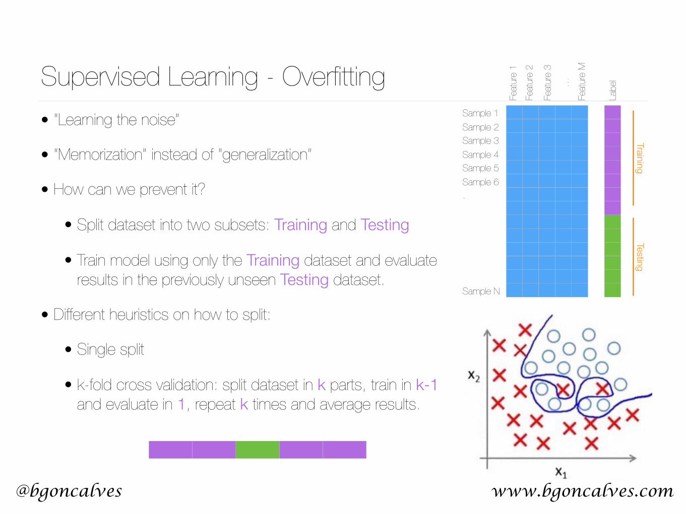
Supervised Learning - OverfittingSample 1Sample 2Sample 3 Sample 4 Sample 5 Sample 6 .
Sample N
Featu
re 1
Featu
re 3
Featu
re 2
…
Labe
l
Featu
re M
• “Learning the noise”
• “Memorization” instead of “generalization”
• How can we prevent it?
• Split dataset into two subsets: Training and Testing
• Train model using only the Training dataset and evaluate results in the previously unseen Testing dataset.
• Different heuristics on how to split:
• Single split
• k-fold cross validation: split dataset in k parts, train in k-1 and evaluate in 1, repeat k times and average results.
TrainingTesting
www.bgoncalves.com@bgoncalves
Supervised Learning - OverfittingSample 1Sample 2Sample 3 Sample 4 Sample 5 Sample 6 .
Sample N
Featu
re 1
Featu
re 3
Featu
re 2
…
Labe
l
Featu
re M
• “Learning the noise”
• “Memorization” instead of “generalization”
• How can we prevent it?
• Split dataset into two subsets: Training and Testing
• Train model using only the Training dataset and evaluate results in the previously unseen Testing dataset.
• Different heuristics on how to split:
• Single split
• k-fold cross validation: split dataset in k parts, train in k-1 and evaluate in 1, repeat k times and average results.
TrainingTesting

www.bgoncalves.com@bgoncalves
Bias-Variance Tradeoff

www.bgoncalves.com@bgoncalves
Bias-Variance Tradeoff
Model Complexity
Erro
r TrainingTesting VarianceBias
High Bias Low Variance
Low Bias High Variance

www.bgoncalves.com@bgoncalves
K-nearest neighbors
• Perhaps the simplest of supervised learning algorithms
• Effectively memorizes all previously seen data
• Intuitively takes advantage of natural data clustering
• Define that the class of any datapoint is given by the plurality of it’s k nearest neighbors
• It’s not obvious how to find the right value of k

www.bgoncalves.com@bgoncalves
K-nearest neighbors
www.bgoncalves.com@bgoncalves
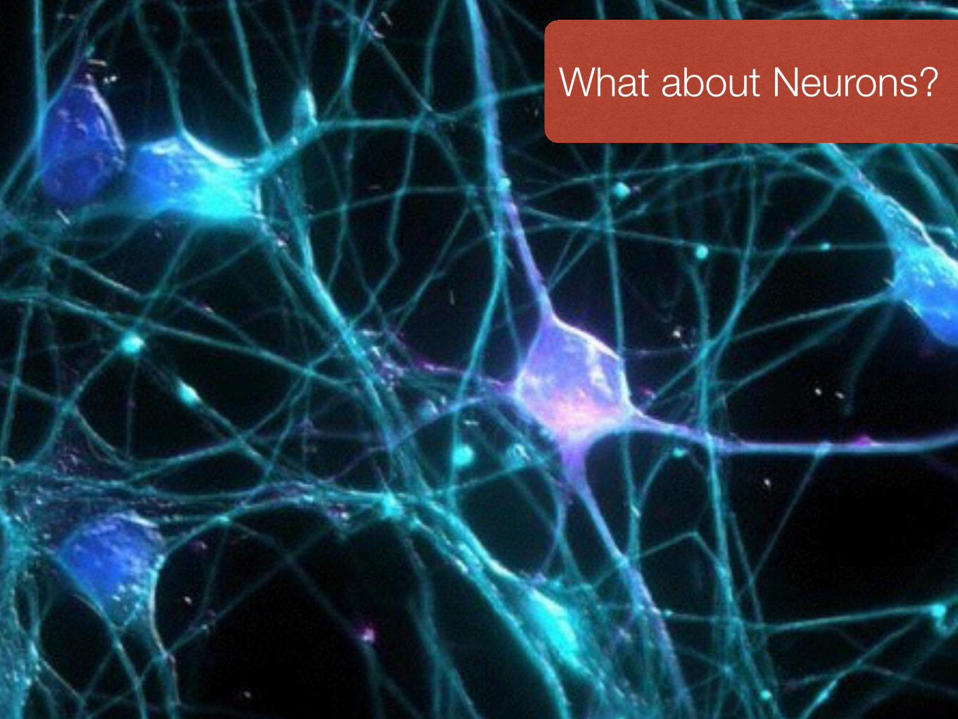
Biological Neuron What about Neurons?

www.bgoncalves.com@bgoncalves
How the Brain “Works” (Cartoon version)

www.bgoncalves.com@bgoncalves
How the Brain “Works” (Cartoon version)• Each neuron receives input from other neurons• 1011 neurons, each with with 104 weights• Weights can be positive or negative• Weights adapt during the learning process• “neurons that fire together wire together” (Hebb)• Different areas perform different functions using same structure (Modularity)

www.bgoncalves.com@bgoncalves
How the Brain “Works” (Cartoon version)
Inputs Outputf(Inputs)

www.bgoncalves.com@bgoncalves
Historical Perspective
1958
Perceptron
• Popularized by F. Rosenblatt who wrote “Principles of Neurodynamics"• Still used today• Simple but limited training procedure• Single Layer

www.bgoncalves.com@bgoncalves
Perceptron
x1
x2
x3
xN
w1j
w2j
w3j
wNj
zjw
Tx
aj� (z)
w0j
1
Inputs Weights OutputActivation function
Bias

www.bgoncalves.com@bgoncalves
Activation Function

www.bgoncalves.com@bgoncalves
Activation Function

www.bgoncalves.com@bgoncalves
Activation Function

www.bgoncalves.com@bgoncalves
Activation Function
� (z) =1
1 + e�z

www.bgoncalves.com@bgoncalves
Activation Function
� (z) =ez � e�z
ez + e�z

@bgoncalves
Activation Functionimport matplotlib.pyplot as plt import numpy as np
def linear(z): return z
def binary(z): return np.where(z > 0, 1, 0)
def relu(z): return np.where(z > 0, z, 0)
def sigmoid(z): return 1./(1+np.exp(-z))
def tanh(z): return np.tanh(z)
z = np.linspace(-6, 6, 100)
plt.style.use('ggplot')
plt.plot(z, linear(z), 'r-') plt.xlabel('z') plt.title('Linear activation function') plt.savefig('linear.png') plt.close() activation.py

www.bgoncalves.com@bgoncalves
Perceptron
x1
x2
x3
xN
w1j
w2j
w3j
wNj
aj
w0j
1
�
�w
Tx
�
Training Procedure:
• If correct, do nothing
• If output incorrectly outputs 0, add input to weight vector
• if output incorrectly outputs 1, subtract input to weight vector
• Guaranteed to converge, if a correct set of weights exists
• Given enough features, perceptrons can learn almost anything
• Specific Features used limit what is possible to learn

www.bgoncalves.com@bgoncalves
Historical Perspective
1958
Marvin Minsky
• Co-authors “Perceptrons” with Seymour Papert • XOR Problem • Perceptrons can’t learn non-linearly separable functions • The first “AI Winter”
Perceptron1969

www.bgoncalves.com@bgoncalves
Historical Perspective
1958Perceptron
1969XOR
1986
Geoff Hinton
• Discovers “Backpropagation”• “Multi-layer Perceptron”• Expensive computation requiring lots of data• Impractical

www.bgoncalves.com@bgoncalves
Forward Propagation• The output of a perceptron is determined by a sequence of steps:
• obtain the inputs
• multiply the inputs by the respective weights
• calculate output using the activation function
• To create a multi-layer perceptron, you can simply use the output of one layer as the input to the next one.
• But how can we propagate back the errors and update the weights?
x1
x2
x3
xN
w1j
w2j
w3j
wNj
aj
w0j
1
�
�w
Tx
�
1
w0k
w1k
w2k
w3k
w Nk
ak��wTa
�
a1
a2
aN
www.bgoncalves.com@bgoncalves
Backward Propagation of Errors (BackProp)• BackProp operates in two phases:
• Forward propagate the inputs and calculate the deltas
• Update the weights
• The error at the output is the squared difference between predicted output and the observed one:
• Where is the real output and is the predicted one.
• For inner layers there is no “real output”!
t
E = (t� y)2
y

www.bgoncalves.com@bgoncalves
Chain-rule• From the forward propagation described above, we know that the
output of a neuron is:
• But how can we calculate how to modify the weights ?
• We take the derivative of the error with respect to the weights!
• Using the chain rule:
• And finally we can update each weight in the previous layer:
• where is the learning rate
yj = �
�w
Tx
�
@E
@wij=
@E
@yj
@yj@wij
wij
@E
@wij
wij � wij � ↵@E
@wij
yj
↵

www.bgoncalves.com@bgoncalves
Learning Rate
Epoch
High Learning RateVery High Learning Rate
Loss Low Learning Rate
Best Learning Rate

www.bgoncalves.com@bgoncalves
Backprop
• Back propagation solved the fundamental problem underlying neural networks
• Unfortunately, computers were still too slow for large networks to be trained successfully
• Also, in many cases, there wasn’t enough available data

www.bgoncalves.com@bgoncalves
Historical Perspective
1958Perceptron
1969XOR
1986
Yann LeCun
• Starts working on Convolutional Neural Networks
• (Eventually) develops the first practical application of image recognition
Backprop1989

www.bgoncalves.com@bgoncalves
Historical Perspective
1958Perceptron
1969XOR
1986
Vladimir Vapnik• Support Vector Machines
• A clever variation on Perceptrons
• Kernel Trick
Backprop1989
ConvNet1995

www.bgoncalves.com@bgoncalves
Support Vector Machine
0
3.25
6.5
9.75
13
0 5 10 15 20
Perceptrons find a hyperp lane that separates the two classes of data

www.bgoncalves.com@bgoncalves
Support Vector Machine
0
3.25
6.5
9.75
13
0 5 10 15 20
But how can we find the hyperplane w i t h t h e b e s t separation of the data?

www.bgoncalves.com@bgoncalves
Support Vector Machines
• Decision plane has the form:
• We want for points in the “positive” class and for points in the negative class. Where the “margin” is as large as possible.
• Normalize such that and solve the optimization problem: subject to:
• The margin is:
w
Tx = 0
w
Tx � b
w
Tx �b
2b
minw
||w||2
yi
�w
Tx
�> 1
2
||w||
b = 1

www.bgoncalves.com@bgoncalves
Kernel “trick”• SVM procedure uses only the dot products of vectors and never the vectors themselves.
• We can redefine the dot product in any way we wish.
• In effect we are mapping from a non-linear input space to a linear feature space

www.bgoncalves.com@bgoncalves
Historical Perspective
1958Perceptron
1969XOR
1986Backprop
1989ConvNet
1995SVM
Geoff Hinton
• Deep Neural Networks• Combines backprop
with faster machines and larger datasets
2006

www.bgoncalves.com@bgoncalves
Neural Network Architectures

www.bgoncalves.com@bgoncalves
Convolutional Neural Networks

www.bgoncalves.com@bgoncalves
Interpretability

www.bgoncalves.com@bgoncalves
“Deep” learning