A Practical Handbook for Population Viability Analysis · A Practical Handbook for Population...

A Practical Handbook forPopulation Viability Analysis

William Morris, Daniel Doak, Martha Groom, Peter Kareiva,

John Fieberg, Leah Gerber, Peter Murphy, and Diane Thomson

Saving the Last Great Places

William Morris1,2, Daniel Doak3,4, Martha Groom5, Peter Kareiva5,

John Fieberg6, Leah Gerber7, Peter Murphy2, and Diane Thomson4.

Evolution, Ecology and Organismal Biology Group1 and Dept. of Zoology2

Duke University, Box 90235, Durham, NC 27708-0325

Biology Board3 and Environmental Studies Board4

University of California, Santa Cruz, CA 95064

Dept. of Zoology5

Box 351800, University of Washington, Seattle, WA 98195-1800

Biomathematics Program6

North Carolina State University, Raleigh, NC 27695

Dept. of Ecology, Evolution, and Marine Biology7

University of California Santa Barbara, Santa Barbara, CA 93106

April 1999

A Practical Handbook forPopulation Viability Analysis

ACKNOWLEDGMENTS

The authors thank Craig Groves for helping to organize the workshop out of which this handbook

grew, the staff of the National Center for Ecological Analysis and Synthesis in Santa Barbara, CA, for

logistical assistance, and Nicole Rousmaniere for designing the final version. The workshop was

generously supported by grants from the Moriah Fund and the David B. Smith Foundation. We also

thank all the workshop participants for providing data sets, and for the enthusiasm and dedication

with which they approach the task of preserving biological diversity. Finally, we thank Christopher

Clampitt, Doria Gordon, Craig Groves, Elizabeth Crone, Larry Master, Wayne Ostlie, Lance

Peacock, Ana Ruesink, Cheryl Shultz, Steve Sutherland, Jim Thorne, Bob Unnasch, Douglas Zollner,

and students in W. Morris’s Fall 1998 graduate seminar at Duke University for reading and

commenting on drafts of the handbook.

A Practical Handbook for Population Viability Analysis

Copyright 1999 The Nature Conservancy

ISBN: 0-9624590-4-6

On the cover: photograph copyright S. Maka/VIREO.

i

CHAPTER ONEWhat Is Population Viability Analysis, and Why This Handbook? ............................ 1

CHAPTER TWOLetting the Data Determine an Appropriate Method for PopulationViability Analysis .............................................................................................. 4

CHAPTER THREEUsing Census Counts Over Several Years to Assess Population Viability .................... 8

CHAPTER FOURProjection Matrix Models ................................................................................. 30

CHAPTER FIVEPopulation Viability for Multiple Occurrences, Metapopulations,and Landscapes ............................................................................................. 48

CHAPTER SIXMaking Monitoring Data Useful for Viability Analysis. ......................................... 65

CHAPTER SEVENReality Check: When to Perform (and When Not to Perform) aPopulation Viability Analysis ............................................................................ 70

REFERENCES ................................................................................................ 75

TABLE OF CONTENTS

1

The 1997 document Conservation by Design: A

Framework for Mission Success states that the con-

servation goal of The Nature Conservancy is “the

long-term survival of all viable native species

and community types through the design and

conservation of portfolios of sites within eco-

regions.” In an ideal world, conservation orga-

nizations like TNC would seek to preserve

every location that harbors a rare, threatened,

or endangered species. But in the real world,

financial considerations make this strategy im-

possible, especially given the number of spe-

cies whose status is already cause for concern.

Thus it is an inescapable fact that for all but the

rarest of species, TNC will need to focus on

preserving only a subset of the known popula-

tions, and upon this choice will rest the suc-

cess of the entire mission. To make this choice,

Conservancy staff require the means to find an-

swers, at the very least qualitative and condi-

tional ones, to two critical questions. First, what

is the likelihood that a known population of a

species of conservation concern will persist for

a given amount of time? Second, how many

populations must be preserved to achieve a rea-

sonable chance that at least one of them will

avoid extinction for a specified period of time?

The goal of this handbook is to introduce prac-

tical methods for seeking quantitative answers

to these two questions, methods that can pro-

vide some guidance in the absence of highly

detailed information that is unlikely to be avail-

able for most rare species. The use of such meth-

ods has come to be known as population

viability analysis (PVA).

Broadly defined, the term “population via-

bility analysis” refers to the use of quantitative

methods to predict the likely future status of a

population or collection of populations of con-

servation concern. Although the acronym PVA

is now commonly used as though it signified a

single method or analytical tool, in fact PVAs

range widely both in methods and applications.

Among the most influential PVAs to date is one

of the original analyses of Northern Spotted Owl

data (Lande 1988). This work relied upon quite

simple demographic data, and its main points

were that logging could result in owl popula-

tion collapse and that the data available at that

time were insufficient to determine how much

forest was needed for the owl population to per-

sist. This second point is important, as it em-

phasizes that PVAs can be highly useful even

when data are sparse. Another influential PVA

(Crouse et al. 1987) used a more complex size-

structured model to assess the status of logger-

head sea turtles and to ask whether protecting

nestlings on beaches or preventing the death of

older turtles in fishing trawls would have a

greater effect on enhancing population recovery.

This single PVA played a critical role in sup-

porting legislation to reduce fishing mortality of

CHAPTER ONEWhat is Population Viability Analysis, and Why ThisHandbook?

2


turtles (Crowder et al. 1994). More recent PVAs

have involved yet more complex spatial mod-

els, for example of individual Lead-beater’s Pos-

sums (Lindemeyer and Possingham 1994). Fur-

thermore, while most PVAs are ultimately con-

cerned with assessing extinction risks, they are

often motivated by the need to address specific

problems, for example sustainable traditional

use levels of forest palms (Ratsirarson et al. 1996),

the risks posed by different poaching techniques

to wild ginseng populations (Nantel et al. 1996),

or loss of movement corridors (Beier 1993). The

uniting theme of PVAs is simply that they all are

quantitative efforts to assess population health

and the factors influencing it.

This handbook grew out of a workshop held

at the National Center for Ecological Analysis

and Synthesis in Santa Barbara, CA, in Febru-

ary, 1998, in which ecologists from four univer-

sities (the authors of this handbook) and TNC

practitioners came together to explore how quan-

titative methods from the field of population bi-

ology might be used to inform TNC decision

making. Prior to the workshop, TNC participants

were asked to supply data sets that exemplify

the types of information that TNC or Heritage

employees and volunteers would collect about

species of conservation concern. In Chapter 2,

we classify the data sets into 3 categories, which

we then use as a starting point to identify a few

quantitative methods that we describe in detail

in the subsequent chapters. In Chapters 3 and

4, we review methods for assessing viability

of single populations when the data represent

census counts or demographic information

about individuals, respectively. In Chapter 5, we

address the question of how to assess regional

viability when a species is distributed across mul-

tiple populations of varying size and “quality”.

We begin with two important caveats. First,

this handbook does not attempt to review the

field of population viability analysis as a whole,

but instead focuses on the subset of all available

PVA methods that we deemed, through our in-

teractions with TNC biologists, to be the most

practical given the types of data typically avail-

able. Second, population viability analyses, be-

cause they are typically based upon limited data,

MUST be viewed as tentative assessments of cur-

rent population risk based upon what we now

know rather than as iron-clad predictions of

population fate. Thus, as we will argue repeat-

edly below, we should not put much faith in the

exact predictions of a single viability analysis

(e.g. that a certain population will have a 50%

chance of persisting for 100 years). Rather, a better

use of PVA in a world of uncertainty is to gain

insight into the range of likely fates of a single

population based upon 2 or more different analy-

ses (if possible), or the relative viability of 2 or

more populations to which the same type of

analysis has been applied. When data on a par-

ticular species are truly scarce, performing a PVA

may do more harm than good. In such cases,

basing conservation decisions on other methods

(e.g. the known presence/absence of a species

at a suite of sites, or its known habitat require-

ments) makes far better sense. We discuss the

question of when NOT to perform a PVA in

greater detail in the final chapter of this hand-

book. Thus, while we view PVA as a potentially

useful tool, we do not see it as a panacea.

3

Chapter One

While data scarcity is a chronic problem

facing all decision making in conservation, we

should also recognize that it is often feasible to

collect additional data to better inform viability

assessments. Indeed, TNC and Heritage person-

nel are constantly collecting new information

in the course of monitoring sites for rare and

threatened species. Simple counts of the num-

ber of individuals of a certain species at a site

over a number of years are often made with other

purposes in mind, but they can also serve as

grist for a population viability analysis. We hope

that awareness of the possible use of monitor-

ing data in PVA will lead TNC/Heritage biolo-

gists to consider ways that their monitoring

schemes can maximize the usefulness of moni-

toring data for future viability assessments, with-

out entailing costly changes in existing moni-

toring protocols. In Chapter 6 of this handbook,

we make easy-to-follow recommendations for

how the design of monitoring strategies can best

meet the data requirements of PVA.

Before proceeding to the consideration of

typical TNC data sets, we say a brief word about

the structure of this handbook. To illustrate the

application of each method, we provide step-

by-step examples, usually using one of the TNC/

Heritage data sets. These worked examples are

featured in Key Boxes that are set aside from

the background text of the handbook. We also

use Key Boxes to highlight key assumptions or

caveats about each of the methods we review.

While the Key Boxes emphasize the methods

we have found to be the most practical, it is

also important to point out that more complex

population viability analyses may be possible

in cases in which more data are available. Be-

cause we do not have the space to thoroughly

review these more complex (and therefore less

frequently useful) analyses in a handbook of

this length, we have also included Optional

Boxes that give a brief overview of other meth-

ods and provide references that will allow the

interested reader to learn more about them.

Finally, we make one further point of clari-

fication. In this handbook, we aim to quantify

the likelihood of persistence of a population (that

is the collection of individuals of a single spe-

cies living in a prescribed area) or a set of popu-

lations over a specified time period. We use the

terms “population” and “element occurrence” (or

“EO”) interchangeably. Thus we use “EO” to re-

fer to a population of a single species, which we

realize is a more restricted usage of the term than

the one used by TNC/Heritage biologists, which

defines elements as “viable native species AND

communities” (see Conservation by Design). We

emphasize that the methods we review are NOT

intended to be used to determine the long-term

viability of communities. However, we note that

PVAs targeted at populations of dominant or

characteristic species in a particular community

type may serve as useful tools for evaluating the

viability of community occurrences.

4

The first rule of population viability analysis is:

“let the data tell you which analysis to perform”.

While population biologists have developed a

vast array of complex and mathematically sophis-

ticated population models, it is our view that

when data are limited (as they almost always will

be when we are dealing with the rare, seldom-

studied species that are the typical concern of

conservation planners) the benefits of using com-

plex models to perform population viability analy-

ses will often be illusory. That is, while more

complex models may promise to yield more

accurate estimates of population viability because

they include more biological detail (such as

migration among semi-isolated populations, the

CHAPTER TWOLetting the Data Determine an Appropriate Method forPopulation Viability Analysis

effects of spatial arrangement of habitat patches,

and the nuances of genetic processes such as

gene flow and genetic drift), this gain in accu-

racy will be undermined if the use of a more

complex model requires us to “guess” at critical

components about which we have no data.

Instead, our philosophy is that the choice of mod-

els and methods in PVA should be determined

primarily by the type of data that are available,

and not the other way around.

With this philosophy in mind, and to get

an idea of the kinds of data that TNC biologists

will typically have at their disposal to perform

population viability analyses, we asked work-

shop participants to provide us with data sets

FIGURE 2.1Characteristics of 20 data sets on rare species considered in the PVA Workshop (see Table 2.1 forinformation on the species included)

0

5

10

15

20

25

0 2 4 6 8 10 12 14

Number of years

Num

ber

of o

ccur

ence

s (s

ites)

CountsDemographic DataPresence/Absence Data

5

Chapter Two

that had been collected in conjunction with TNC

field offices. We received 26 data sets, which

included information about 25 species of con-

servation concern. We classified these data sets

according to the type of data, the number of lo-

cations, and the number of years in which data

were collected. By “type of data”, we mean

whether the persons who collected the data

recorded the PRESENCE OR ABSENCE of the

species at a location, COUNTS of individuals

in one or more life stages, or DEMOGRAPHIC

information about individual organisms (that is,

whether each individual survived from one cen-

sus to the next and if so, its size at each census

and the number of offspring it produced in the

time interval between the censuses).

This survey of data sets highlights four pat-

terns (Table 2.1, Fig. 2.1). First, count data is

the most common type of information in this

sample of TNC data sets. Second, relatively long

duration studies tended to focus on only a single

site, while multi-site studies typically involved

Species Type of No. of No. ofData sites years

Shale barren rockcress, Arabis serotina Counts 1 6

Shale barren rockcress, Arabis serotina Counts 17 3

Dwarf trillium, Trillium pusillum Counts 1 4

Eriocaulon kornickianum Counts 1 3

Mesa Verde cactus, Sclerocactus mesae-verdae Counts 1 10

Mancos Milkvetch, Astragalus humillimus Counts 1 8

Knowlton’s cactus, Pediocactus knowltonii Counts 1 11

Lesser prairie chicken, Tympanuchus pallidicinctus Counts 1 13

Seabeach pinweed, Amaranthus pumilus Counts 18 8

Golden Alexanders, Zizia aptera Counts 1 7

Oenothera organensis Counts 8 2

Arizona stream fish (7 species) Counts 1 1

Red-cockaded woodpecker, Picoides borealis Counts 2 12

Bog turtle, Chlemmys muhlenbergii Counts 7 3

Kuenzler hedgehog cactus, Demographic 1 2Echinocereus fendleri var. kuenzleri

Ornate box turtle, Terrapene ornata Demographic 1 8

Larimer aletes, Aletes humilis Demographic 2 7

Mead’s milkweed, Asclepias meadii Demographic 1 4

Trollius laxus Demographic 1 3

Cave salamander, Gyrinophilus palleucus Presence/Absence 20 1

TABLE 2.1 Data sets contributed to the TNC PVA workshop

6


TABLE 2.2 A classification of PVA methods reviewed in this handbook

Number of Type of data Minimum number PVA method: Where topopulations collected: of years of data look in thisor EOs included per population handbook:in the analysis: or EO:

One Counts 10 (preferably more) Count-based Chapter 3extinctionanalysis

One Demographic 2 or more Projection Chapter 4information matrix models

More Than One Counts 10 (preferably more) Multi-site Chapter 5for at least one extinctionof the populations analysis

only one or a few censuses, which is not sur-

prising given the limited resources available to

monitor populations of conservation concern.

Only one of the 26 data sets included informa-

tion from more than 8 sites in more than 3 years.

Third, demographic data sets, because they are

more difficult to collect, tend to include fewer

years on average than do count data. Fourth,

the data set that included the most sites com-

prised presence/absence data. The single ex-

ample of presence/absence data here surely

underestimates the true frequency of such data

sets in Heritage data bases. While information

about presence/absence of a species is critically

important in identifying high-priority sites for

acquisition or preservation (Church et al. 1996,

Pressey et al. 1997), such data sets lack the popu-

lation-level details required for a PVA, and we

do not address them further in this handbook.

To the extent that this informal sample gives

a rough idea of the types of data accessible to

TNC biologists, it suggests three themes about

how PVA might best serve TNC decision making

processes. First, our informal survey of data sets

shows that counts of the number of individuals

in one or more populations over multiple years

will be the most common information upon

which population viability analyses will need to

be based, but that in some cases (most likely for

umbrella or indicator species, and those for which

particular reserves have been especially estab-

lished) more detailed analyses based upon

demographic information will be feasible.

Second, while information will sometimes be

available to perform PVAs on multiple local popu-

lations, most decisions about the number of

occurrences needed to safeguard a species will

require extrapolation from information collected

at only one or a few populations at best. Third,

the kinds of information that are missing from

these data sets is also noteworthy. None of them

include any information about genetic processes

or, in the case of data sets that include multiple

occurrences, about rates of dispersal of individuals

among populations. Thus we conclude that more

complex models that require this information

7

Chapter Two

will not be justified in most cases. We reiterate

these themes in the following chapters.

Thus Fig. 2.1 suggests three general classes

of data sets that provide information that can be

used to perform a PVA:

- Counts of individuals in a single popu-

lation obtained from censuses performed over

multiple years;

- Detailed demographic information on

individuals collected over 3 or more years

(typically at only 1 or 2 sites); and

- Counts from multiple populations, in-

cluding a multi-year census from at least one

of those populations.

Each of these classes require somewhat

different methods for population viability analy-

sis. Fortunately, population biologists have

developed methods to deal with each of these

situations. Table 2.2 summarizes the data

requirements for PVA based upon each of these

three classes of data, and points to where each

type of PVA is presented in this handbook.

8

As we saw in Chapter 2 (Fig. 2.1), the type of

population-level data that is most likely to be

available to conservation planners and manag-

ers is count data, in which the number of indi-

viduals in either an entire population or a sub-

set of the population is censused over multiple

(not necessarily consecutive) years. Such data

are relatively easy to collect, particularly in com-

parison with more detailed demographic infor-

mation on individual organisms (see Chapter

4). In this chapter, we review an easy-to-use

method for performing PVA using count data.

The method’s simplicity makes it applicable

to a wide variety of data sets. However, several

important assumptions underlie the method,

and we discuss how violations of these assump-

tions would introduce error into our estimates

of population viability. We also point to other,

similar methods that can be employed in the

face of biological complexities that make the

simpler method less appropriate.

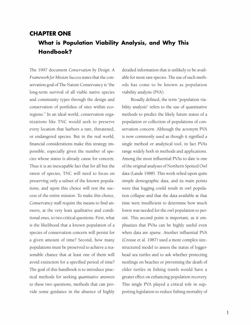
In a typical sequence of counts from a

population, the numbers do not increase or de-

crease smoothly over time, but instead show

considerable variation around long-term trends

(see examples in Fig. 3.1). One factor that is

likely to be an important contributor to these

fluctuations in abundance is variation in the

environment, which causes the rates of birth

and death in the population to vary from year

to year. The potential sources of environmen-

tally-driven variation are too numerous to list

CHAPTER THREEUsing Census Counts Over Several Years to AssessPopulation Viability

fully here, but they include inter-annual varia-

tion in factors such as rainfall, temperature, and

duration of the growing season. Most popula-

tions will be affected by such variation, either

directly or indirectly through its effects on in-

teracting species (e.g. prey, predators, competi-

tors, diseases, etc.). When we use a sequence

of censuses to estimate measures of population

viability, we must account for the pervasive ef-

fect of environmental variation that can be seen

in most count data. To see how this is done, we

first give a brief overview of population dynam-

ics in a random environment, and then return

to the question of how count data can be used

to assess population viability.

Population dynamics in a random

environment

Perhaps the simplest conceptual model of

population growth is the equation

Equation 3.1

N(t+1) = λ N(t),

where N(t) is the number of individuals in the

population in year t, and λ is the population growth

rate, or the amount by which the population mul-

tiplies each year (the Greek symbol “lambda” is

used here by tradition). If there is no variation in

the environment from year to year, then the popu-

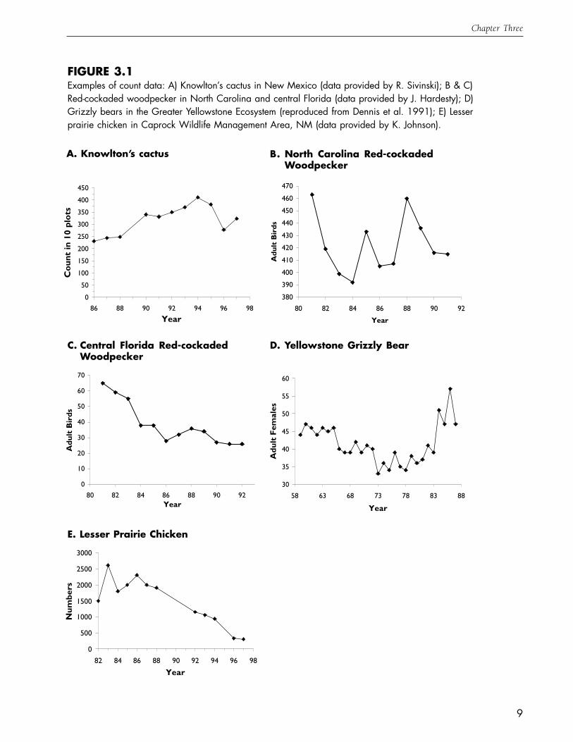
lation growth rate λ is a constant, and only three

qualitative types of population growth are pos-

sible (Fig. 3.2A): if λ is greater (continued on page 11)

9

Chapter Three

FIGURE 3.1Examples of count data: A) Knowlton’s cactus in New Mexico (data provided by R. Sivinski); B & C)Red-cockaded woodpecker in North Carolina and central Florida (data provided by J. Hardesty); D)Grizzly bears in the Greater Yellowstone Ecosystem (reproduced from Dennis et al. 1991); E) Lesserprairie chicken in Caprock Wildlife Management Area, NM (data provided by K. Johnson).

A. Knowlton’s cactus B. North Carolina Red-cockadedWoodpecker

0

50

100

150

200

250

300

350

400

450

86 88 90 92 94 96 98

Year

Cou

nt in

10

plot

s

380

390

400

410

420

430

440

450

460

470

80 82 84 86 88 90 92

Year

Adu

lt B

irds

C. Central Florida Red-cockadedWoodpecker

D. Yellowstone Grizzly Bear

30

35

40

45

50

55

60

58 63 68 73 78 83 88

Year

Adu

lt F

emal

es

0

10

20

30

40

50

60

70

80 82 84 86 88 90 92Year

Adu

lt B

irds

E. Lesser Prairie Chicken

0

500

1000

1500

2000

2500

3000

82 84 86 88 90 92 94 96 98

Year

Num

bers

10


0

10

20

30

40

50

60

70

80

0 5 10 15 20

Time, t

Abu

ndan

ce, N

(t)

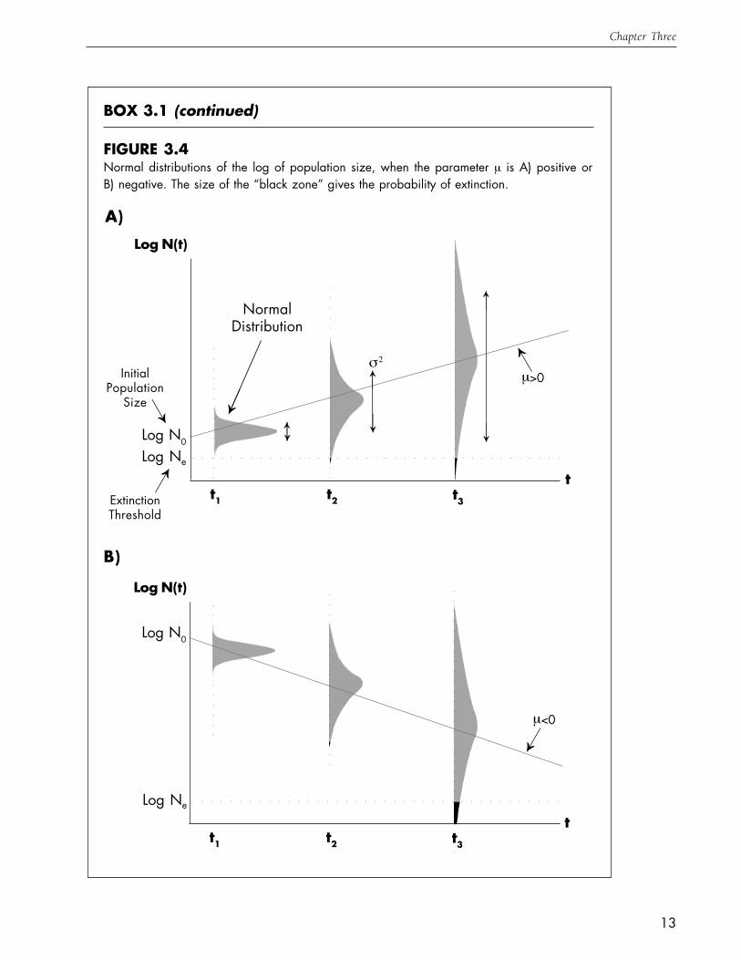
FIGURE 3.2Population growth described by a geometric growth model N(t+1) = λN(t) in (A) a constant or (B)a stochastically-varying environment

A. No Environmentally-Driven Variability

B. Populations in a Stochastic Environment

➊

➋

➌➝

➝

➝

0

5

10

15

20

25

30

0 5 10 15 20

Time, t

Abun

danc

e, N

(t) !>1

!=1

!<1

11

Chapter Three

than one, the population grows geometrically; if λ

is less than one, the population declines geometri-

cally to extinction; and if λ exactly equals one, the

population neither increases nor declines, but re-

mains at its initial size in all subsequent years. But

when variation in the environment causes survival

and reproduction to vary from year to year, the

population growth rate λ must also be viewed as

varying over some range of values. Moreover, if

the environmental fluctuations driving changes in

population growth include an element of

unpredictability (as factors such as rainfall and

temperature are likely to do), then we must face

the fact that we cannot predict with certainty what

the exact sequence of future population growth

rates will be. As a consequence, even if we know

the current population size and both the average

value and the degree of variation in the popula-

tion growth rate λ, the best we can do is to make

probabilistic statements about the number of indi-

viduals the population will include at some time

in the future. To illustrate, Fig. 3.2B shows a hy-

pothetical population governed by the same equa-

tion we saw above, but in which the value of the

population growth rate λ in each year was gener-

ated on a computer so as to vary randomly around

an average value. Each line in the figure can be

viewed as a separate “realization” of population

growth, or a possible trajectory the population

might follow given a certain average value and

degree of variability in λ.

Fig. 3.2B illustrates three important points

about population growth in a random or “sto-

chastic” environment. First, the possible real-

izations of population growth diverge over time,

so that the farther into the future predictions

about likely population size are made, the less

precise they become. Second, the realizations

do not follow very well the predicted trajectory

based upon the average population growth rate.

In particular, even though the average λ in this

case would predict that the population should

increase at a slow rate, a few realizations ex-

plode over the 20 years illustrated, while others

decline (thus extinction is possible even though

the average of the possible population trajecto-

ries increases). Third, the endpoints of the 20

realizations shown are highly skewed, with a

few trajectories (such as ➌) winding up much

higher than the average λ would suggest, but

most (such as ➊) ending below the average. This

skew is due in part to the multiplicative nature

of population growth. Because the size of the

population after 20 years depends on the prod-

uct of the population growth rate in each of

those years, a long string of chance “good” years

(i.e. those with high rates of population growth)

would carry the population to a very high level

of abundance, while “bad” years tend to con-

fine the population to the restricted zone be-

tween the average and zero abundance.

Skewness in the distribution of the likely

future size of a population is a general feature of

a wide variety of models of population growth in

a stochastic environment. In fact, we can make

the even more precise statement that for many

such models, the endpoints of multiple indepen-

dent realizations of population growth will lie

approximately along a particular skewed prob-

ability distribution known as the log-normal,

or equivalently that the natural log of popula-

tion size will be normally (continued on page 14)

12


BOX 3.1 (Optional): Theoretical Underpinnings

Probability Distributions Describing Population Size in aRandomly Varying Environment

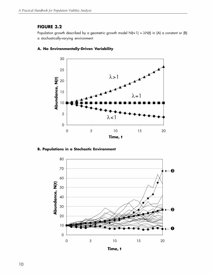
We saw in Fig. 3.2B that possible realizations of population growth in a stochastic environment becomeskewed, with a few high-abundance realizations outweighed by a large number of low-abundancerealizations. If we were to simulate a large number of such realizations and then divide them into abundance“bins” at several different times, we would get the following sequence of histograms (Fig. 3.3), whichclearly shows the skewness in population abundance. Note that with the passage of time, both the averagevalue and the degree of spread in these histograms increases. If we make the size of the “bins” smaller andsmaller, the histograms in Fig. 3.3 will come to resemble the skewed probability distribution known as thelog-normal. If abundance has a log-normal distribution, then the natural log of abundance will have anormal distribution, whose mean and variance will also change over time (Fig. 3.4). Measures of populationviability are derived directly from this shifting normal distribution. For example, the probability that thepopulation lies below the threshold at a certain time is simply the area under the normal distribution belowthe threshold (shown in red in Fig. 3.4). The time until the threshold is first attained is also determined bythe normal distribution (see Box 3.3). The shifting normal distribution is completely described by twoparameters. The parameter µ determines how quickly the mean in-creases (if µ is greater than zero, Fig.3.4A) or decreases (if µ is less than zero, Fig. 3.4B). The second parameter, σ2, determines how quickly thevariance in the normal distribution increases. Clearly if µ is less than zero, extinction is certain, but even if

µ is positive (i.e. the populationis expected to grow on average),there will be some chance thatthe population falls below thethreshold, particularly if the vari-ance increases rapidly (i.e. if σ2 islarge). Thus to measure a popu-lation’s risk of extinction, wemust know the values of bothµ and σ2.

FIGURE 3.3Log-normal distributions of abundance in a population grow-ing exponentially in a stochastic environment

t = 5

0.0

0.1

0.2

0.3

2.5

7.5

12.5

17.5

22.5

27.5

32.5

37.5

42.5

47.5

52.5

57.5

62.5

67.5

72.5

77.5

t =10

0.0

0.1

0.2

0.3

t =15

0.0

0.1

0.2

0.3

Mid

poin

t of

Abu

ndan

ce C

ateg

ory

t = 20

0.0

0.1

0.2

0.3

Fraction of Population Realizations

13

Chapter Three

BOX 3.1 (continued)

A)

Log N(t)

t

B)

FIGURE 3.4Normal distributions of the log of population size, when the parameter µ is A) positive orB) negative. The size of the “black zone” gives the probability of extinction.

Log N0

Log Ne

InitialPopulation

Size

ExtinctionThreshold

→

→

NormalDistribution

→ µ>0

→

→

→

→→

→

→

σ2

t1 t2 t3

Log N(t)

tt1 t2 t3

µ<0→

Log N0

Log Ne

14


distributed (see Box 3.1). This important result

means that we can use the normal distribution

(whose properties are well understood, as it

underlies much of modern statistical theory) to

calculate measures of viability, such as the prob-

ability that the population will be above some

threshold size a given number of years into the

future, or the likely number of years before the

population first hits the threshold. But before we

can calculate these measures, we must first esti-

mate two parameters that describe how the nor-

mal distribution of the log of population size will

change over time: µ, which governs change in

the mean of the normal distribution, and σ2, which

governs how quickly the normal distribution’s

variance will increase over time (Box 3.1). Both

of these parameters will have important effects

on measures of population viability, so we require

a method to estimate their values using count data.

Using count data to estimate

population parameters

Brian Dennis and colleagues (Dennis et al.

1991) have proposed a simple method for esti-

mating µ and σ2 from a series of population

censuses. The method involves two easy steps:

1) calculating simple transformations of the

counts and of the years in which counts were

taken, and 2) performing a linear regression

(Box 3.2). The results of the regression yield

estimates of µ and σ2.

Measures of viability based upon

! and "2

Once we have estimated the parameters µ

and σ2 from count data, we can calculate several

measures of the viability of the population from

which the counts were obtained (Box 3.3). One

is the average value of the population growth

rate, λ. This value indicates whether the average

of the possible population trajectories will tend

to increase (λ>1), decrease (λ<1), or remain the

same (λ=1) over one census interval (thus λ de-

scribes ➋ in Fig. 3.2B). Keep in mind that some,

or even most, realizations of population growth

may decline even if their average increases (see

Fig. 3.2B). The confidence interval for λ is also

informative, because only if the entire confidence

interval lies above or below the value 1 can we

say (for example with 95% confidence) that the

average of population trajectories will increase

or decrease, respectively.

Because the average value of the popula-

tion growth rate doesn’t do a good job of pre-

dicting what most population realizations will

do, two other viability measures, the mean time

to extinction and the probability that extinction

has occurred by a certain future time, may be

calculated. These require us to specify an initial

population size (typically the most recent count)

and an “extinction” threshold. The “extinction”

threshold need not be set at zero abundance.

For a non-hermaphroditic species, we may wish

to set the threshold at 1, at which point the

population would be effectively extinct. It may

be reasonable to set the threshold at even higher

levels, such as the abundance at which genetic

drift or demographic stochasticity reach a pre-

determined level of importance, or the lowest

level of abundance at which it remains feasible

to attempt intervention to prevent further de-

cline. Once we arrive at an (continued on page 17)

15

Chapter Three

BOX 3.2 (Key): Methods of AnalysisEstimating Useful Parameters from a Series of Population Censuses

Dennis et al. (1991) outlined the following simple method to estimate the parameters µ and σ2 from aseries of counts from a population:■ First, choose pairs of counts N(i) and N(j) from adjacent censuses i and j performed in

years t(i) and t(j).■ Second, calculate the transformed variables x = √t( j )-t( i) and

y = ln(N(j)/N(i))/√t( j )-t( i) = ln(N(j)/N( i))/x for each pair.■ Third, use all the resulting pairs of x and y to perform a linear regression of y on x, forcing the

regression line to have a y-intercept of zero (Fig. 3.5).The slope of the resulting regression line is an estimate of the parameter µ. The mean squared residual,which can be read from the Analysis of Variance table associated with the regression, is an estimate of theparameter σ2.

As an illustration of the method, the following data were collected in a monitoring study of thefederally-listed Knowlton’s cactus (Pediocactus knowltonii) made over 11 years by R.L. Sivinski at itsonly known location in San Juan County, New Mexico (see Fig. 3.1A). The data are summed counts ofthe number of individual plants in ten permanent 10 square meter plots (an eleventh plot was omittedbecause all the individuals were removed in 1996 by cactus poachers!). The transformed variables xand y are also shown. Note that an advantage of the Dennis et al. method is that it does not require thatcensuses be performed year after year without fail. For example, monitoring of

FIGURE 3.5The regression of y on x for the Knowlton’s cactus data. The slope of the regression line is anestimate of µ, and the variance of the points around the line is an estimate of σ2

(continued on page 16)

-0.4

-0.3

-0.2

-0.1

0

0.1

0.2

0.3

0 0.5 1 1.5

x= (t(j) - t(i))

y=ln

(N(j)

/N(i)

)/

(t(j)

-t(i)

)

!

!

16


BOX 3.2 (continued)

1986 231

1987 √(1987-1986) = 1 244 ln(244/231)/1 = 0.054751

1988 1 248 0.016261

1990 1.414 340 0.223104

1991 1 331 -0.02683

1992 1 350 0.055815

1993 1 370 0.05557

1994 1 411 0.10509

1995 1 382 -0.07317

1996 1 278 -0.3178

1997 1 323 0.150031

Year x=!t(j)-t(i) Count y=ln(N(j)/N(i)/x

Knowlton’s cactus was incomplete in 1989, and omitting that census results in adjacent counts in 1988and 1990 that are 2 years apart. We simply use an x value of √2 = 1.414 and a y value of ln(340/248)/√2 for that pair of counts in the regression.

Once x and y have been calculated, the linear regression can be performed by any statistical pack-age or even by basic spreadsheet programs. The following output was produced using Microsoft Excel(with the Analysis Toolpak installed) to perform a linear regression on the transformed Knowlton’scactus data above (and forcing the y-intercept to be zero by checking the “Constant is Zero” option inthe Regression window):

First check to see that the circled number ➊ is zero; if not, you failed to check the “Constant isZero” box, and must redo the regression. The circled number ➋!is the slope of the linear regression,which provides an estimate of the parameter µ. The circled number ➌ in the ANOVA table is the meansquared residual, which is an estimate of σ2. For Knowlton’s cactus, these estimates indicate that µ ispositive and σ2 is less than µ, as is expected given that the counts show an increasing trend without a

Coefficients Standard Error t Stat P-value Lower 95% Upper 95%

Intercept 0.00000 #N/A #N/A #N/A #N/A #N/A

X Variable 1 0.03048 0.04377 0.69631 0.50382 -0.06853 0.12949

➊

➋

ANOVA

df SS MS F Significance F

Regression 1 0.00432 0.00432032 0.20502671 0.662721138

Residual 9 0.189648 0.021072

Total 10 0.193968

➌

17

Chapter Three

great deal of inter-annual variability (Fig. 3.1A). In contrast, the estimated µ and σ2 for the lesser prairiechicken (Fig. 3.1E) are -0.106 and 0.097, respectively; the negative value of µ reflects the sharp declineof this population.

Note that the last column of the ANOVA table above indicates that this is a non-significant regres-sion (p>0.05). This should not deter us from using our estimated µ and σ2 to calculate viability mea-sures; we are using linear regression here to find the best-fit values of the parameters given the data, notto statistically test any particular hypotheses.

Regression methods also allow one to detect outliers (years of unusually high population growthor unusually steep decline) in the count data. If these outliers coincide with events such as a change inthe census protocol or one-time human impacts (e.g. oilspills) that are unlikely to recur, we may wishto omit them when estimating µ and σ2. One can also test statistically whether µ and σ2 differed beforeand after a management strategy was instituted or a permanent change in the environment took place.Interested readers should consult Dennis et al. (1991).

BOX 3.2 (continued)

appropriate threshold, based upon biological,

political, and economic considerations, we can

define a population above the threshold to be

viable, and can calculate both the mean time to

attain the threshold given that it is reached and

the probability that the population has fallen

below the threshold by a specified time in the

future (Box 3.3).

Because it is relatively easy to calculate,

much theoretical work has focused on the mean

time until an extinction threshold is reached.

But we must be careful here, because the mean

time to extinction will almost always overestimate

the time it takes for most doomed realizations to

reach a threshold. This fact traces back to the

skewness in population abundance that devel-

ops in a stochastic environment (Fig. 3.2B). The

large fraction of realizations that hover at low

abundance are likely to dip below the threshold

at relatively short times, while the few realiza-

tions that grow rapidly at first will likely take a

very long time before they experience the long

string of bad years necessary to carry them below

the threshold. These later trajectories have a dis-

proportionate effect on the mean time to extinc-

tion. For this reason, the mean time to extinc-

tion is a potentially misleading metric for PVA.

A better measure of the time required for

most populations to attain the threshold is the

median time to extinction, which is one of sev-

eral useful measures that can easily be obtained

from the so-called “cumulative distribution func-

tion,” or CDF, of the conditional time to extinc-

tion (Box 3.3). In effect, the conditional extinc-

tion time CDF asks the question: “if the extinc-

tion threshold is going to be reached eventually,

what is the probability that a population start-

ing at a specified initial size will have already

hit the threshold at a certain time in the fu-

ture?” Thus the conditional extinction time CDF

considers only those population realizations that

will eventually fall below the threshold; this will

include all possible realizations if µ is less than

or equal to zero, but only a subset of realiza-

18


tions if µ is greater than zero (see Box 3.3). When

the estimated value of ! is negative (so that even-

tual extinction is certain), the conditional extinc-

tion time CDF is the single most useful viability

measure one can compute. From the CDF, one

can read the median time to extinction as the

time at which the probability of extinction first

reaches a value of 0.5 (Fig. 3.6); for the reason

given above, the median time to extinction is

typically shorter than the mean time to extinc-

tion. The time to any other “event”, such as the

probability of extinction first exceeding 5% (or

to put it in a more positive light, the probability

of population persistence first falling below

95%), can also be easily read off the CDF. The

CDF also clearly shows the probability of popu-

lation persistence until any given future time

horizon, which itself may be dictated by man-

agement considerations. Even if the estimated

value of ! is positive (so that only a subset of the

possible realizations will ever hit the extinction

threshold), calculating the conditional extinction

time CDF is still valuable, because it can be used

in combination with the

FIGURE 3.6The cumulative distribution function of extinction time for the lesser prairie chicken estimated fromthe data in Fig. 3.1E. Arrows indicate how the CDF can be used to calculate: A) the median time toextinction given that extinction occurs (note that the median, 29 years, is less than the mean time toextinction of 32.1 years); B) the probability of extinction by 100 years; and C) the number of yearsat which there is only a 5% chance of population persistence.


Lesser Prairie Chicken

0.0

0.1

0.2

0.3

0.4

0.5

0.6

0.7

0.8

0.9

1.0

0 50 100 150 200

Time (years)

Cum

ulativ

e Pr

obabili

ty o

f Ex

tinct

ion

A

C

B

19

Chapter Three

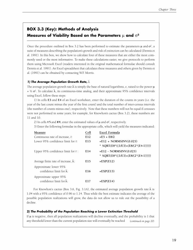
BOX 3.3 (Key): Methods of AnalysisMeasures of Viability Based on the Parameters ! and "2


Measure Cell Excel FormulaContinuous rate of increase, r: E12 =E5 + E8/2Lower 95% confidence limit for r: E13 =E12 + NORMSINV(0.025)

* SQRT(E8*((1/E3)+(E8/(2*(E4-1)))))

Upper 95% confidence limit for r : E14 =E12 - NORMSINV(0.025)* SQRT(E8*((1/E3)+(E8/(2*(E4-1)))))

Average finite rate of increase, λ: E15 =EXP(E12)

Approximate lower 95%confidence limit for λ: E16 =EXP(E13)

Approximate upper 95%confidence limit for λ: E17 =EXP(E14)

Once the procedure outlined in Box 3.2 has been performed to estimate the parameters µ and σ2, asuite of measures describing the population’s growth and risk of extinction can be calculated (Dennis etal. 1991). In this box, we show how to calculate four of these measures that are either the most com-monly used or the most informative. To make these calculations easier, we give protocols to performthem using Microsoft Excel (readers interested in the original mathematical formulae should consultDennis et al. 1991). An Excel spreadsheet that calculates these measures and others given by Dennis etal. (1991) can be obtained by contacting W.F. Morris.

1) The Average Population Growth Rate, "The average population growth rate λ is simply the base of natural logarithms, e, raised to the power µ+ ! σ2. To calculate λ, its continuous-time analog, and their approximate 95% confidence intervalsusing Excel, follow these steps:

1) In cells E3 and E4 of an Excel worksheet, enter the duration of the counts in years (i.e. theyear of the last count minus the year of the first count) and the total number of inter-census intervals(the number of counts minus one), respectively. Note that these numbers will not be equal if censuseswere not performed in some years; for example, for Knowlton’s cactus (Box 3.2), these numbers are11 and 10.

2) In cells and , enter the estimated values of µ and σ2, respectively.3) Enter the following formulae in the appropriate cells, which will yield the measures indicated:

For Knowlton’s cactus (Box 3.6, Fig. 3.1A), the estimated average population growth rate λ is1.04 with a 95% confidence of 0.96 to 1.14. Thus while the best estimate indicates the average of thepossible population realizations will grow, the data do not allow us to rule out the possibility of adecline.

2) The Probability of the Population Reaching a Lower Extinction ThresholdIf µ is negative, then all population realizations will decline eventually, and the probability is 1 thatany threshold lower than the current population size will eventually be reached

20


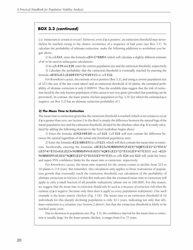
BOX 3.3 (continued)

(i.e. extinction is certain to occur). However, even if µ is positive, an extinction threshold may never-theless be reached owing to the chance occurrence of a sequence of bad years (see Box 3.1). Tocalculate the probability of ultimate extinction, make the following additions to worksheet you be-gan above:

1) In cell E11, enter the formula =(E4-1)*E8/E4, which will calculate a slightly different estimateof σ2 to be used in subsequent calculations.

2) In cells E19 and E20, enter the current population size and the extinction threshold, respectively.3) Calculate the probability that the extinction threshold is eventually reached by entering the

formula =IF(E5<0,1,(E20/E19)^(2*E5/E11)) in cell E22.For Knowlton’s cactus, the estimate of m is positive (Box 3.2), and using a current population size

of 323 (the size of the last count taken) and an extinction threshold of 10 plants, the estimated prob-ability of ultimate extinction is only 0.000014. Thus the available data suggest that the risk of extinc-tion faced by the only known population of this cactus is not very great (provided that poaching can beprevented). In contrast, the lesser prairie chicken population in Fig. 3.1E (for which the estimated µ isnegative; see Box 3.2) has an ultimate extinction probability of 1.

3) The Mean Time to ExtinctionThe mean time to extinction given that the extinction threshold is reached (which is not certain to occurif µ is greater than zero; see Section 2 in this Box) is simply the difference between the natural logs of theinitial population size and the extinction threshold, divided by the absolute value of µ. It is easily calcu-lated by adding the following elements to the Excel worksheet begun above:

1) Enter the formula =LN(E19/E20) in cell E21. Cell E21 will now contain the difference be-tween the natural logarithms of the initial and threshold population sizes.

2) Enter the formula =E21/ABS(E5) in cell E23, which will then contain the mean time to extinc-tion. Incidentally, entering the formulae =IF(E23+NORMSINV(0.025)*SQRT((E21^2)*E$11/((E5^4)*E3))<0,0,(E23+NORMSINV(0.025)*SQRT((E21^2)*E11/((E5^4)*E3)))) and =E23-NORMSINV(0.025)*SQRT((E21^2)*E11/((E5^4)*E3)) in cells E24 and E25 will yield the lowerand upper 95% confidence limits for the mean time to extinction, respectively.

For Knowlton’s cactus, the mean time required for the census counts to decline from 323 to10 plants is 114 years. But remember, this calculation only applies to those realizations of popula-tion growth that eventually reach the extinction threshold; our calculation of the probability ofultimate extinction in Section 2 of this Box indicates that the estimated mean time to extinction willapply to only a small fraction of all possible realizations (about one in 100,000). For this reason,we suggest that the mean time to extinction should only be used as a measure of extinction risk when theestimate of µ is negative (because only then does it apply to every population realization). One suchexample is the lesser prairie chicken (Fig. 3.1E). The mean time to an extinction threshold of 10individuals for this sharply declining population is only 32.1 years, indicating not only that ulti-mate extinction is a certainty (see Section 2 above), but that the extinction threshold is likely to bereached quite soon.

Due to skewness in population size (Fig. 3.3), the confidence interval for the mean time to extinc-tion is usually large; for the lesser prairie chicken, it ranges from 0 to 77 years.

21

Chapter Three

BOX 3.3 (continued)

4) The Cumulative Distribution Function (CDF) for the Conditional Time to ExtinctionNext, we can extend our Excel worksheet to calculate the conditional extinction time CDF given thatthe extinction threshold will be attained. The extinction time CDF gives the probability, considering onlythose realizations of population change that ultimately fall below the extinction threshold, that the thresholdhas already been reached at a given time. Hence as with the mean time to extinction, the extinction timeCDF applies to all realizations if µ<0, but to only a subset of realizations if µ>0. To calculate it, we usethe standard normal cumulative distribution function NORMSDIST provided by Excel:

1) Fill column B downward from cell B31 with a series of times at which you wish to computethe CDF. For most purposes, every 5 years from 5 to 1000 years is adequate (the sequence “Edit-Fill-Series” from the pull-down menu will allow you to accomplish this easily).

2) In cell D31, enter the following formula:=NORMSDIST((-$E$21+ABS($E$5)*$B31)SQRT($E$11*$B31))+EXP(2*$E$21*ABS ($E$5)/$E$11)*NORMSDIST((-$E$21-ABS($E$5)*$B31)/SQRT($E$11*$B31)).Now select cell , drag downward to the row corresponding with the last entry in Column B that youcreated in step 2, and then type Ctrl-D; column D will now be filled with the values of the CDF thatcorrespond to the times in Column B. You can treat these 2 columns as a table in which you can look upvalues of the CDF at different times, or you can use Excel to create a graph of the CDF versus time (forexample, Fig. 3.6 shows a graph of the CDF for the lesser prairie chicken, and indicates how severalmeasures of population viability (including the median time to extinction) can be read from the graph).

5) Using the Extinction Time CDF When ! is PositiveWhen µ is positive, the extinction time CDF must be interpreted with caution, because it does not applyto all population realizations (only to those that will eventually reach the extinction threshold). For ex-ample, the median time to extinction from the CDF (not shown) for the Knowlton’s cactus populationin Fig. 3.1A is 105 years (using a current population size of 323 and an extinction threshold of 10plants). This does NOT mean that half of all realizations will have reached the extinction threshold by105 years, but instead that half of the realizations that will eventually hit the threshold (which represent onlyabout 1 in 100,000 possible realizations) will have done so by 105 years. Given the positive value of µ, theunderlying population model predicts that the remaining 99,999 of 100,000 realizations will NEVERhit the extinction threshold. Nevertheless, the conditional extinction time CDF is still valuable evenwhen µ is positive, for the following reason. We can calculate the total probability that the population hasgone extinct by a given future time horizon, accounting for ALL possible realizations, if we calculate boththe probability that the extinction threshold is reached eventually (see Section 2 of this Box) and theconditional extinction time CDF. The total probability that extinction occurs by, say, 100 years is theprobability that extinction will occur eventually multiplied by the conditional probability that extinctionwill have occurred by 100 years given that it will occur eventually, which is precisely what the conditionalextinction time CDF tells us. For Knowlton’s cactus, the value of the CDF at 100 years is 0.455, so thetotal probability of reaching an extinction threshold of 10 plants by 100 years is 0.000014 (see Section2 above) multiplied by 0.455, or 0.0000064, a rather small number. By performing a calculation such asthis, we could compare the relative viabilities of two populations, one with postive and one with nega-tive µ, whereas it would be inappropriate to compare directly the CDFs of the two populations.

22


probability of ultimate extinction to compute the

likelihood that extinction will have occurred by a

given future time horizon (see Box 3.3).

Uses of the Extinction Time Cumulative

Distribution Function in Site-based and

Ecoregional Planning

Because the conditional extinction time CDF

encapsulates so much useful information about

population viability, we now give three examples

that show how the CDF can be used to inform

decisions about the viability of individual ele-

ment occurrences (EOs), or about which of sev-

eral EOs should receive the highest priority for

acquisition or management.

Perhaps the most valuable use of the CDF

is to make comparisons between the relative

viabilities of 2 or more EOs. Ideally, we would

have a series of counts from each EO. For

example, Fig. 3.1B & C show the number of

adult birds during the breeding season in popu-

lations of the federally-listed red-cockaded

woodpecker in central Florida and in North

Carolina. Applying the methods outlined in

Boxes 3.2 and 3.3 yields the CDFs in Fig. 3.7A.

Both because it has a more negative estimate for

µ (-0.083 vs -0.011) and a smaller initial size,

the Florida population has a much greater prob-

ability of extinction at any future time than does

the North Carolina population.

Often we will not have independent census

data from each EO about which we must make

conservation decisions. However, if we have a

single count of the number of individuals of a

particular species in one EO, we can use count

data from multiple censuses of the same species

at a second location to make a provisional

viability assessment for the first EO when no other

data are available. For example, Dennis et al.

(1991) calculated the extinction time CDF for

the population of grizzly bears (Ursus arctos) in

the Greater Yellowstone ecosystem, using values

of µ and σ2 estimated from aerial counts of the

number of adult females over 27 years, a starting

population of 47 females (the number estimated

in 1988, the last census available to them), and

an “extinction” threshold of 1 female (Fig 3.7B).

A second isolated population of grizzly bears

occupying the Selkirk Mountains of southern

British Columbia consists of about 20 adults, or

roughly 10 adult females. If we have no infor-

mation about the Selkirk Mountains population

other than its current size, we may as well use

the CDF for the Yellowstone population to give

us a relative sense of the viability of the Selkirks

population. In so doing, we are assuming that

the environments (including the magnitude of

inter-annual variation) and the human impacts

at the two locations are similar, an assumption

which could be evaluated using additional in-

formation on habitat quality, climatic variation,

and land-use patterns. Accepting these assump-

tions, and using the CDF from the Yellowstone

population, the Selkirks population of 10 females

would have an 31-fold greater probability of

extinction at 100 years (Fig 3.7B; for an exten-

sion of this analysis to multiple sites, see Box

5.2). For species of particular concern, it may

be possible to improve upon this approach by

compiling count data from multiple locations.

We could then estimate average values for the

parameters µ and σ2 to provide ballpark assess-

23

Chapter Three

FIGURE 3.7How to use the extinction time CDF in site-based and ecoregional planning. A) Comparing the CDF’sfor the two red-cockaded woodpecker populations in Fig. 3.1B, C (for both curves, initial populationsize equaled the last available count and the extinction threshold was 10 birds). B) CDF’s for theYellowstone grizzly bear (Fig. 3.1D) assuming initial population sizes of 10 or 47 females and anextinction threshold of 1 female; C) The effect of the variance parameter σ2 on the CDF, using thedata for the Yellowstone grizzly bear with the observed variance (σ2=0.9) or one half the observedvariance (σ2=0.45)

A) Red-cockadedWoodpecker

B) YellowstoneGrizzly Bear

C) YellowstoneGrizzly Bear

0.0

0.1

0.2

0.3

0.4

0.5

0.6

0.7

0.8

0.9

1.0

0 100 200 300 400 500 600 700 800 900 1000

Time (years)

Cum

ulat

ive

Prob

abili

ty o

f Ex

tinct

ion

10 Females

47 Females

0

0.1

0.2

0.3

0.4

0.5

0.6

0.7

0.8

0.9

1

0 100 200 300 400 500

Time (years)

Cum

ulat

ive

Prob

abili

ty o

f Ex

tinct

ion

0.0

0.1

0.2

0.3

0.4

0.5

0.6

0.7

0.8

0.9

1.0

0 100 200 300 400 500

Time (years)

Cum

ulat

ive

Prob

abili

ty o

f

Extin

ctio

n

σ2=0.45

σ2=0.9

CentralFlorida

NorthCarolina

24


ments of viability for EOs with only a single cen-

sus, or choose the location with the most similar

environment for comparison.

As a final use of the CDF, we point out that

even in the absence of any count data for a spe-

cies of critical concern, knowledge of how the

CDF is affected by its underlying parameters can

help us to make qualitative assessments of relative

viability, especially if we can use natural history

information to make inferences about the local

environment of an EO or about the life history of

the species in question. For example, we will fre-

quently be able to make an educated guess that

one EO’s environment is likely to be more vari-

able than another’s in ways that will affect popu-

lation growth. Similarly, some species will have

life history features (e.g. long-lived adults) that

buffer their populations against year-to-year en-

vironmental variation. If the effects of environ-

mental variation on the population growth rate

are less for one species or EO than another, then

its σ2 value will be smaller. Such differences in σ2

influence the CDF even when its other determi-

nants (µ and the starting and threshold popula-

tion sizes) are fixed (Fig. 3.7C). Thus we can

state that, all else being equal, the greater the en-

vironmentally-driven fluctuations in population

growth rate the greater will be the risk of extinc-

tion at early time horizons, a qualitative statement

that nonetheless provides some useful guidance.

Assumptions in Using the Method of Dennis

et al.

As with any quantitative model of a com-

plex biological process, PVA using count data

relies upon simplifying assumptions. In Box 3.4,

we list the most important assumptions we are

making when we apply the method of Dennis

et al. to a series of counts and then estimate

measures of population viability. The fact that

these assumptions are explicit is an advantage

of a quantitative approach to evaluating viabil-

ity, relative to an approach based upon general

natural history knowledge or intuition. By evalu-

ating whether the assumptions are met, we can

determine whether our analysis is likely to give

unreliable estimates of population viability, but

more importantly, we can often determine

whether violations of the assumptions are likely

to render our estimates (e.g. of time to extinc-

tion) optimistic or pessimistic. By “optimistic”

and “pessimistic”, we mean, for example, that

the true time to extinction is likely to be shorter

or longer than the estimated value, respectively.

If we know that the estimated time to extinc-

tion for an EO is short but pessimistic, we should

be more cautious in assigning a low viability

ranking, while a long but optimistic estimate

should not inspire complacency.

We now give a few brief examples illustrat-

ing how, by evaluating the assumptions in Box

3.4, we can make more informed viability assess-

ments. One life history feature that may cause

Assumption 1 (Box 3.4) to be violated is dor-

mant or diapausing stages in the life cycle, such

as seeds in a seed bank or diapausing eggs or

larval stages of insects and freshwater crustaceans.

Because they are difficult to census accurately,

these stages are typically ignored in population

counts, but as a result the counts may not repre-

sent a constant fraction of the total population.

For example, when the number of above-ground

25

Chapter Three

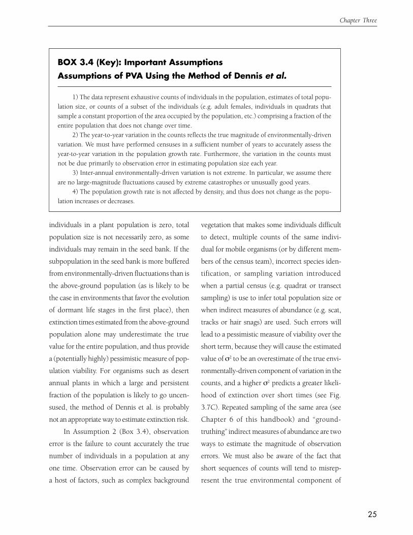
BOX 3.4 (Key): Important AssumptionsAssumptions of PVA Using the Method of Dennis et al.

1) The data represent exhaustive counts of individuals in the population, estimates of total popu-lation size, or counts of a subset of the individuals (e.g. adult females, individuals in quadrats thatsample a constant proportion of the area occupied by the population, etc.) comprising a fraction of theentire population that does not change over time.

2) The year-to-year variation in the counts reflects the true magnitude of environmentally-drivenvariation. We must have performed censuses in a sufficient number of years to accurately assess theyear-to-year variation in the population growth rate. Furthermore, the variation in the counts mustnot be due primarily to observation error in estimating population size each year.

3) Inter-annual environmentally-driven variation is not extreme. In particular, we assume thereare no large-magnitude fluctuations caused by extreme catastrophes or unusually good years.

4) The population growth rate is not affected by density, and thus does not change as the popu-lation increases or decreases.

individuals in a plant population is zero, total

population size is not necessarily zero, as some

individuals may remain in the seed bank. If the

subpopulation in the seed bank is more buffered

from environmentally-driven fluctuations than is

the above-ground population (as is likely to be

the case in environments that favor the evolution

of dormant life stages in the first place), then

extinction times estimated from the above-ground

population alone may underestimate the true

value for the entire population, and thus provide

a (potentially highly) pessimistic measure of pop-

ulation viability. For organisms such as desert

annual plants in which a large and persistent

fraction of the population is likely to go uncen-

sused, the method of Dennis et al. is probably

not an appropriate way to estimate extinction risk.

In Assumption 2 (Box 3.4), observation

error is the failure to count accurately the true

number of individuals in a population at any

one time. Observation error can be caused by

a host of factors, such as complex background

vegetation that makes some individuals difficult

to detect, multiple counts of the same indivi-

dual for mobile organisms (or by different mem-

bers of the census team), incorrect species iden-

tification, or sampling variation introduced

when a partial census (e.g. quadrat or transect

sampling) is use to infer total population size or

when indirect measures of abundance (e.g. scat,

tracks or hair snags) are used. Such errors will

lead to a pessimistic measure of viability over the

short term, because they will cause the estimated

value of σ2 to be an overestimate of the true envi-

ronmentally-driven component of variation in the

counts, and a higher σ2 predicts a greater likeli-

hood of extinction over short times (see Fig.

3.7C). Repeated sampling of the same area (see

Chapter 6 of this handbook) and “ground-

truthing” indirect measures of abundance are two

ways to estimate the magnitude of observation

errors. We must also be aware of the fact that

short sequences of counts will tend to misrep-

resent the true environmental component of

26


variability, because they will tend not to include

extreme values.

One violation of the assumptions that will

cause viability estimates to be optimistic is the

existence of intermittent catastrophes (Assump-

tion 3), such as rare ice storms, droughts, severe

fires, etc., which introduce the possibility of sud-

den declines in abundance not accounted for

in our estimate of σ2. More detailed methods

have been developed to include catastrophes in

estimates of time to extinction (see the methods

of Mangel and Tier 1993 and Ludwig 1996,

which also allow density dependence; see be-

low). However, with most short-term count data,

we will lack sufficient information to estimate

the frequency and severity of rare catastrophes,

information that more detailed methods require

if they are to provide more accurate assessments

of extinction time. Thus in practice, we may

need to be content with the statement that if

catastrophes do indeed occur, our assessments

of extinction risk based upon short-term census

data will likely underestimate the true risk. If

catastrophes do occur but with similar intensity

and frequency across multiple EOs, we can still

use the method of Dennis et al. to assess relative

viability. Of course the converse, failure to ac-

count for rare good years, will have a pessimis-

tic effect on the estimated extinction risk.

The ways in which density dependence

(i.e., the tendency for population growth rate to

change as density changes; see Assumption 4)

may alter our estimates of extinction risk are

more complex. A decline in the population

growth rate as density increases will tend to keep

the population at or below a carrying capacity.

Unlike the predictions of the geometric growth

model upon which the viability measures of

Dennis et al. are based, such regulated popula-

tions cannot grow indefinitely, and the prob-

ability of ultimate extinction is always 1 (al-

though the time to extinction may be extremely

long). On the other hand, declining populations

may receive a boost as density decreases and

resources become more abundant; because esti-

mates of µ based upon counts taken during the

decline do not account for this effect, they may

result in pessimistic estimates of extinction risk.

Finally, the opposite effect may occur if a de-

cline in density leads to difficulties in mate find-

ing or predator defense and a consequent re-

duction in population growth rate. The down-

ward spiral created by these so-called “Allee ef-

fects” results in extinction risks that become

greater and greater as the population declines,

and causes estimates of extinction risk made by

ignoring these effects to be overly optimistic.

As with catastrophes, including density de-

pendence in viability assessments will generally

require more data, but there are ways to do so.

Statistical methods developed by Pollard et al.

(1987) and by Dennis and Taper (1994) allow

one to test whether the counts show any evi-

dence of density dependence (but see Shenk et

al. 1998). If the population growth rate does de-

pend upon density, density-dependent versions

of the geometric growth equation 3.1 can be fit

to the count data, using nonlinear rather than

linear regression techniques (Middleton and

Nisbet 1997). However, it is an inescapable fact

that, because density-dependent models require

us to estimate at least three parameters (for

27

Chapter Three

example, the carrying capacity in addition to µ

and σ2), they will require more censuses to achieve

a similar degree of estimation accuracy. In addi-

tion, for most density-dependent population

growth models, there are no simple mathemati-

cal formulae for extinction probability or time to

extinction, and we must rely upon computer

simulations to calculate them (for example, see

Ludwig 1996 and Middleton and Nisbet 1997).

One exception that has received a great deal of

attention from theoretical population biologists

is a model in which the population grows expo-

nentially up to a ceiling, above which it cannot

go. In this case, mathematical formulae for the

mean time to extinction have been derived by

several authors (Box 3.5). Examining the rela-

tionship between time to extinction and the

“height” of the population ceiling provides a way

to ask how the maximum population size a par-

ticular EO will support should influence its rank

(Box 3.5).

BOX 3.5 (Optional): Theoretical UnderpinningsDensity-Dependent Models

When a population’s growth rate declines with increasing density, the population will not continue togrow exponentially, but will typically approach a carrying capacity, usually denoted K. A mathemati-cally simple way to approximate this effect is to allow the population to grow exponentially until itreaches K, when further population growth ceases. This model of “exponential growth up to a ceiling”allows us to ask how the mean time to extinction of a population currently at the ceiling increases as theceiling itself increases. Because the “height” of the ceiling will be determined by the amount of habitatavailable to the population, this is another way of asking how the spatial extent of an EO will influencepopulation viability. Approximate formulae for relationship between the mean time to extinction andthe height of the population ceiling have been derived by several authors, including Lande (1993),Foley (1994), and Middleton et al. (1995).

Here we give a brief overview of the results of Lande (1993). When the parameter µ is positive,the mean of the normal distribution of the log of population size will increase over time (Fig. 3.4); thatis, most population realizations will grow. Nevertheless, some realizations will fall below the extinctionthreshold, and this outcome will be more likely if σ2 is large. In fact, the magnitude of the environmen-tally-driven variation in the population growth rate, as embodied by the parameter σ2, will have apervasive effect on how the extinction time depends on the height of the population ceiling, K. Landeshowed that if µ is positive and the ceiling is sufficiently high, the mean time to extinction will beapproximately proportional to K2µ/σ2. The ratio of µ to σ2 thus determines the shape of the relationshipbetween the mean time to extinction and the population ceiling (Fig. 3.8). If σ2 is small relative to µ (i.e.less than 2µ), the extinction time increases faster than linearly as the ceiling is increased; increasing σ2

until it equals and then surpasses 2µ will cause the scaling of extinction time vs height of the ceiling tobecome linear and then less-than-linear. Thus if environmental variability is high, we may face a law ofdiminishing returns; by increasing the ceiling (for example by increasing the amount of habitat avail-able to the population), we may gain a disproportionately small increase in the (continued on page 28)

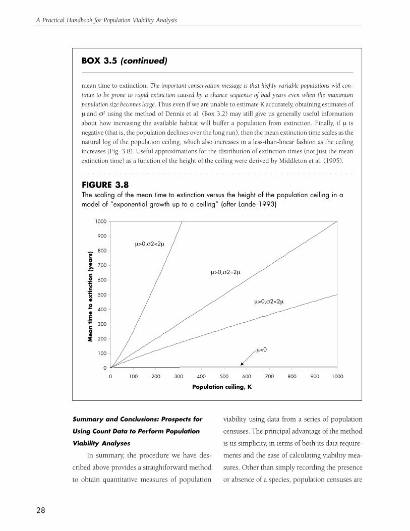
28


FIGURE 3.8The scaling of the mean time to extinction versus the height of the population ceiling in amodel of “exponential growth up to a ceiling” (after Lande 1993)

BOX 3.5 (continued)

Summary and Conclusions: Prospects for

Using Count Data to Perform Population

Viability Analyses

In summary, the procedure we have des-

cribed above provides a straightforward method

to obtain quantitative measures of population

viability using data from a series of population

censuses. The principal advantage of the method

is its simplicity, in terms of both its data require-

ments and the ease of calculating viability mea-

sures. Other than simply recording the presence

or absence of a species, population censuses are

mean time to extinction. The important conservation message is that highly variable populations will con-tinue to be prone to rapid extinction caused by a chance sequence of bad years even when the maximumpopulation size becomes large. Thus even if we are unable to estimate K accurately, obtaining estimates ofµ and σ2 using the method of Dennis et al. (Box 3.2) may still give us generally useful informationabout how increasing the available habitat will buffer a population from extinction. Finally, if µ isnegative (that is, the population declines over the long run), then the mean extinction time scales as thenatural log of the population ceiling, which also increases in a less-than-linear fashion as the ceilingincreases (Fig. 3.8). Useful approximations for the distribution of extinction times (not just the meanextinction time) as a function of the height of the ceiling were derived by Middleton et al. (1995).

0

100

200

300

400

500

600

700

800

900

1000

0 100 200 300 400 500 600 700 800 900 1000

Population ceiling, K

Mea

n tim

e to

ex

tinct

ion

(yea

rs)

µ>0,σ2<2µ

µ>0,σ2=2µ

µ>0,σ2<2µ

µ<0

29

Chapter Three

likely to be the simplest way that field biologists

can collect data. However, to apply the methods

described above, censuses must be conducted

over a reasonable number of years. We recommend

that ten censuses should be viewed as an absolute mini-

mum when applying this method, and more would be

preferable (see Chapter 7). But when an adequate

number of censuses are available, both the linear

regression and the calculation of viability mea-

sures such as the extinction time CDF can be

performed in short order using software avail-

able on almost any desktop computer.

Users of count-based PVA need to be aware

of its limitations when the underlying assump-

tions (Box 3.4) are violated. Because of these

limitations, the method we have presented here

is not a panacea for making conservation deci-

sions in a world of sparse data, but neither are

these limitations a fatal flaw that renders the

method unusable. We reiterate that because the

assumptions are explicit, the exercise of calcu-

lating the extinction time CDF (for example) is

still useful, because we will often be able to

gauge in which direction our estimate is in error

(something which cannot always be said about

viability measures obtained in other ways, such

as through expert opinion). Moreover, if we

know that a particular factor (such as density

dependence in the population growth rate) has

been omitted in a consistent way across mul-

tiple PVAs, they may still provide us with useful

guidance about how risks are likely to differ

among species or EOs. In essence, we argue that

count-based PVA is best viewed as a tool that

provides us with relative measures of the “health”

of two or more populations, measures that deci-

sion-making agendas such as ecoregional plan-

ning require us to make. That is, while we would

not put much credence in a particular numeri-

cal value of a viability measure (for example,

the estimated median time to extinction for the

lesser prairie chicken population of 22 years

(Fig. 3.6)), we can be more comfortable accept-

ing that median extinction time estimates of, for

example, 100 and 500 years for two EOs warn

us of potentially real differences in the viability

of those populations. Assessing the reliability of

viability measures when the underlying assump-

tions of the method are violated is currently an

area of active research in population biology.

But at the present time, we believe it would be a

shame not to make use both of the available

data (e.g. Fig. 2.1) and of the simple tools at

hand to bring some quantitative rigor to the

process of determining the relative ranks of mul-

tiple occurrences of rare and unique species.

30

CHAPTER FOURProjection Matrix Models

While simple counts of the number of individu-

als in a population are more likely to be available

(See Chapter 2, Fig. 2.1), for a few species of

particular concern we may have access to

detailed demographic information describing

the rates of survival, reproduction, and growth

of individuals that differ in size, age or other

characteristics. Viability analyses that use such

individual-based data most often rely upon popu-

lation projection matrices. Matrix models pre-

dict long-term population growth rates, transient

population dynamics, and probabilities of extinc-

tion over time. A basic requirement for construct-

ing a projection matrix is that we must be able to

classify individuals unambiguously into classes

based on their age, size or life-history stage. We

must then quantify the survival, growth, and

reproduction of numerous individuals in each

class over a minimum of 2 to 3 years, preferably

longer. These data are used to calculate so-called

“vital rates”, or the class-specific annual rates of

survival, growth and fecundity, as well as the

degree of year-to-year variation in those rates.

In turn, we use the vital rates to compute the

entries in the projection matrix, which we then

use to predict the likely future trajectory of the

population and its risk of extinction.

Projection matrix models have three advan-

tages over simpler models that track only the

total number of individuals in a population, such

as those we reviewed in Chapter 3. (The tradeoff

that balances these advantages is that we require

far more data to construct a projection matrix

than we do to perform a count-based PVA.) First,

projection matrices make it possible to assess the

influence that the vital rates of particular classes

have on the growth of the population as a whole.

For example, it is possible in a matrix analysis to

assess how much juvenile mortality (as distinct

from the mortality of other life stages) drives

population decline. In an analysis based on

total population counts, we would not be able

to discern whether juvenile mortality plays a role

in the decline—we would simply know that the

population is declining. Yet if juvenile mortality

is a key factor causing the decline, management

efforts aimed at improving juvenile survival

should be more effective than efforts aimed at

other vital rates or life stages.

A second advantage to a matrix model is

that it may more accurately predict future popu-

lation trends for a long-lived species that has

undergone either recent changes in one or more

vital rates (e.g. due to a novel human impact,

or a recently-imposed management plan) or a

perturbation in the population structure (i.e.

the distribution of individuals among classes).

For example, if the fecundity of adults suddenly

drops, or if a large number of juveniles unex-

pectedly migrates from the population, counts

of adults may show little change for several

years, despite the fact that the adult population

will certainly decline once the reduced juve-

nile cohort matures. Put another way, count data

31

Chapter Four

for long-lived species can reflect past conditions

more than current ones. If recent changes in

vital rates or population structure have occurred,

more accurate predictions are possible with a

matrix approach.

A third advantage of projection matrix mod-

els is that they are particularly well suited to

evaluating management alternatives, provided

demographic data from contrasting situations

exist. For example, an experiment in which dif-

ferent management techniques are applied ran-

domly to different plots, or data from sites with

different management histories, would facilitate

the construction of contrasting matrices for each

management scenario. These matrices would

serve to integrate the various effects of manage-

ment on multiple vital rates into an overall ef-

fect on population growth. Moreover, manipu-

lation of the parameters in matrix models al-

lows one to perform computer “experiments” to

predict the likely effects of proposed manage-

ment practices. Importantly, these models can

be informative about the magnitude of threats

and the potential for improvements, and allow

determination of how much effort will be nec-

essary to rescue a declining population.

Like count-based models, projection ma-

trix models can also be used to assess the rela-

tive viability of different EOs. The difficulty is

that in order to do this, demographic data must

be collected from several sites. Obviously, only

very rarely will it be possible to undertake this

type of analysis, but at the end of this chapter

we present one example of this comparative

approach using a TNC data set for the rare plant

Aletes humilis.

In this chapter, we describe the construc-

tion and analysis of projection matrix models,

but we do not cover the topic comprehensively

(thorough reviews are given by Caswell (1989)

and Tuljapurkar and Caswell (1997)). There are

a large number of complexities and nuances to

this type of PVA; hence users would be well-

advised to consult with a population modeller to

go beyond the simpler uses of matrix models cov-

ered here. However, it is important to have an

understanding of the principal issues in model

construction and interpretation even if collabo-

rating with a mathematical population biologist.

Constructing and using a projection

matrix model

The most laborious and time-intensive step

in matrix-based modeling is the collection of

demographic data on known individuals over a

number of years. The details of how to gather

such data are well described in a variety of ref-

erences (e.g. Southwood 1978, Krebs 1989), and

we do not review them here. Instead, we de-

scribe in Box 4.1 the steps one must follow to

use raw data on individuals to produce a pro-

jection matrix and to use the matrix to predict

future population sizes. The basic steps are:

STEP 1: Determine what feature of indi-

viduals (age, size, or life stage) best predicts

differences in vital rates. Then divide the popu-

lation into classes based upon the feature you

have chosen.

STEP 2: Use demographic data on known

individuals to estimate the vital rates for each class,

and use them to construct a population matrix,

according to the rules specified in Box 4.1.

32


BOX 4.1 (Key): Methods of AnalysisConstructing and Using a Matrix Model: A Step-by-Step Guide

STEP 1. Decide if the population is best classified by age, size, or life stage.

To put together a model we must first divide the population into different classes. We can do this byAGE (e.g., all individuals a year old, all individuals 2 years old, etc.), SIZE (e.g., all individuals <10 cmlong, all individuals 10-20 cm long, etc.), or STAGE (e.g., all seeds, all seedlings, all saplings, all adults).The choice of which type of classification to use depends on the life history of the organism and on theavailable data.

Age-structured populations: For many species the age of the individual is the best descriptor ofhow the vital rates react to the environment. For example, it could be that 1-yr olds survive worst, and 3-yr olds best. An age-structured matrix is often the method of choice when our data are taken fromknown-age individuals in a cohort analysis. Determinate growers (e.g. mammals and birds) are oftenmodeled in this way, or with a modified formulation which adds a final adult stage. This simplification isonly appropriate for species in which there is little variation in adult survival and fecundity rates as indi-viduals age. Obviously, an age-based classification is restricted to species that are easy to age in the field.

Size-structured populations: If the exact age is not as important as the physical size of an indi-vidual in determining its vital rates, then a size-based model should be used. Examples include plants, forwhich size often influences how many seeds an individual can produce, and many fish species, in whichsize influences survival. Size may also be used when age is unknown, because size can be measured easily

STEP 3: Construct a population vector by

specifying the initial number of individuals in

each class in the population. A population vec-

tor is a list of the number of individuals in each

class; the sum of the elements in the vector

equals the total population size.

STEP 4: Use the matrix and the population

vector to project the population forward in time,

thus predicting the future size of the population,

the long-term population growth rate, λ, and the

risk of future extinction. This step involves simple

rules of linear algebra (Box 4.1, Step 4).

While these simple steps apply to any

matrix-based PVA, there are a host of additional

complexities that may be added to the models,

and many additional analyses that could be

performed. The most essential complexity to be

included in a PVA, provided the data are avail-

able, is year-to-year variation in vital rates. We

discuss this complexity in detail in the follow-

ing section of this chapter. One additional analy-

sis that is usually desirable is to perform

“experiments” by looking at effects on λ and on

extinction risk of altering matrix entries to

reflect changes in the demographic rates of

particular life stages resulting from differing

forms of management. Often this is the most

instructive step in using matrix models. After

we review how to include stochastic variation

into matrix models, we give an example of a

matrix-based PVA using TNC data, illustrating

how projection matrices can be used to explore

management options.


33

Chapter Four

BOX 4.1 (continued)

in the field. Typically, the divisions between size categories are determined by looking for critical sizes atwhich vital rates change abruptly, or by assuring that the number of individuals in the data set that willfall into each size class will be adequate to estimate vital rates (see below).


Stage-structured populations: Organisms in which the life stage of an individual (such as simplybeing a newborn, a juvenile, or a reproductive adult, regardless of age or size within these stages) hasthe greatest influence on vital rates should be modeled as a stage-structured population. Stage-struc-tured models can be the easiest to use because recognizing distinct stages may be more practical thandetermining age or size.

Next we must determine the number of classes to use. This decision must strike a balance be-tween two opposing goals. First, each class should be as homogeneous as possible—that is, all indi-viduals within a class should be quite similar in terms of their vital rates, while differing from individu-als in other classes. Second, the number of individuals in each class must be large enough to estimatevital rates accurately. Using too few classes will cause us to lump in a single class individuals that possessdifferent demographic rates, whereas using too many classes means that some will contain too fewindividuals for accurate estimation of vital rates. See Vandemeer (1979) for one approach to balancingthese two goals.

STEP 2. Construct a projection matrix.

We are now ready to transform raw data into class-specific vital rates, and then put these into a matrixformat. All projection matrices, regardless of the type of classification used, have the form:

1 2 3 4

1 a11 a12 a13 a14

2 a21 a22 a23 a24

3 a31 a32 a33 a34

4 a41 a42 a43 a44

FROM CLASS

TO CLASS

Each matrix entry (a11 - a44) has two subscripts, the first indicating its row and the second indicat-ing its column in the matrix. Each entry corresponds to the annual rate of the transition FROM the classindicated by the column subscript TO the class indicated by the row subscript. Thus a32 is the annualrate of transition from class 2 to class 3. Fecundities are placed in the first row of the matrix becausethey represent contributions from adult classes to the newborn class (which by convention is class 1),and in this case correspond to entries a12, a13, and a14. All other entries in the matrix represent classtransitions of individuals other than newborns (for example a23, a33, and a43 give the fraction of class 3individuals that shrink to class 2, remain the same size, and grow to class 4 in one year, respectively).

The details of taking raw data and calculating the probabilities that go into the matrix arediscussed using two examples.

34


BOX 4.1 (continued)

Example 1: A stage-structured matrix. We will use as our first example a modified age-basedmatrix for the American Oystercatcher, a threatened shorebird that breeds along the eastern and gulfcoasts of the U.S. (from Davis and Groom, unpublished manuscript). American Oystercatchers can bedivided into three stages: juveniles, subadults, and adults. Data on the fates of banded oystercatchers andthe success of known nests have been gathered by a variety of researchers for more than a decade. Ameri-can oystercatchers have very low fecundity due to high rates of nest loss to predators and storm events.Each adult oystercatcher nesting on South Core Banks, NC, produces an average of only 0.054 offspringthat survive to the following year (Davis and Simons 1997). Juvenile survivorship is also low, estimated tobe 66.5% per year. However, adult survivorship is high, and birds may live as long as 20 years. Annualadult and subadult survivorships are estimated to be 95% and 72.4%, respectively.

We have arranged these data on fecundity and survival rates of individuals in each stage into a matrix, (see equation 4.1 below). Fecundity values are placed on the first row, and survival rates are placed in the

other two rows so as to correctly represent transitions from one stage to another (e.g., survival from thesubadult stage to the adult stage (0.724) goes in column 2 (FROM subadults) of row 3 (TO adults):

Example 2: A size-structured matrix. Nantel et al. (1996) performed a PVA to determine theharvest potential of American Ginseng (Panax quinquefolium). Ginseng is a perennial plant that is difficultto age, but individuals vary in their survival and fecundity according to the number of leaves. Hence,plants are divided into 4 size classes, those with 1, 2, 3, and 4 leaves, and into seed and seedling classes.

In the case of a size-structured population, many more transitions among classes are possiblethan in an age-structured or even a stage-structured population, because individuals may grow one ormore size classes in a single year, and may even drop from a larger to a smaller class (many plants, forexample, may shrink between years). To measure the rates at which these numerous transitions occurin the population, it is best to perform a census of marked individuals in all size categories (as was donewith Aletes humilis; see Tables 4.1 and 4.2). We do not have the original data that Nantel et al. used toconstruct their matrices, but we could imagine they followed 100 marked individuals in each size class(including seedlings, which are called the 0 size class) and obtained the following results:

SIZE CLASS WHEN MARKED:

SIZE NEXT YEAR:

0 1 2 3 4

0 0 0 0 0 01 16 25 0 0 02 2 59 52 6 03 0 0 40 85 194 0 0 3 5 74

Equation 4.1 FROM:

TO:

juveniles subadults adults

0 0 0.0540.665 0 00 0.724 0.95

juvenilessubadultsadults

= M

35

Chapter Four

Note that the numbers in each column do not sum to the initial number of marked individuals(due to mortality), that most individuals with 1 leaf grow if they survive, and that shrinkage occursonly rarely (6 individuals with 3 leaves shrank to having just two, and 19 individuals with 4 leavesshrank to having just 3). Fecundity values represent the production by aboveground plants of seeds inthe soil (represented by size class “S”). Estimating fecundities is more complex than estimating othermatrix elements; we discuss the estimation of fecundities in more detail in Box 4.2. In this example,counting the average number of seeds that each marked individual produces during the year is themost straightforward way of calculating fecundity (although these numbers must be corrected for thedeath of seeds between the time they are produced and the time of the next census; see Box 4.2). Theestimated fecundities for ginseng are 0, 0, 1.35, 13.24, and 18.50 surviving seeds per year for classes 0to 4, respectively. Nantel et al. estimated that 9% of seeds survive and emerge as seedlings in the follow-ing year. Using the fecundity estimates in the first row of the matrix, and dividing each number in thetable above by 100 (the initial number of marked ginseng plants in each size class) to get the corre-sponding matrix entries, yields the matrix:

BOX 4.1 (continued)

S 0 1 2 3 4

S 0 0 0 1.35 13.24 18.50

0 .09 0 0 0 0 0

1 0 .16 .25 0 0 0

2 0 .02 .59 .52 .06 0

3 0 0 0 .4 .85 .19

4 0 0 0 .03 .05 .74


Step 3. Construct an initial population vector. The initial population vector is simply acolumn of the numbers of individuals currently in each class. For example, if the oystercatcher popu-lation in Example 1 above has 40 juveniles, 50 subadults, and 60 adults in year t, the population isdescribed by the vector:

nt=405060

The total population size is obtained by adding together the numbers in the vector (so this populationhas a total of 150 individuals).

Step 4. Project the population by multiplying the projection matrix by the popula-tion vector. Projecting the number of individuals in each class one year from now given a currentpopulation vector consists of multiplying the projection matrix by the population vector to generate anew population vector. Multiplication is achieved as follows. For each row of the matrix, take theproduct of the first entry of that row and the first entry of the vector, add that to the product of thesecond entry of that row and the second entry of the vector, and repeat for all

36


BOX 4.1 (continued)

other entries of the row and vector. The result is the first entry in the new population vector. Repeat thisprocess for all other rows of the matrix. For example, to project the oystercatcher population, wemultiply the matrix M (see equation 4.1 above) by the population vector nt:

M x nt = nt+1

(0x40)+(0x50)+(.054x60)

(.665x40)+(0x50)+(0x60)

(0x40)+(.724x50)+(.95x60)

0 0 .054

.665 0 0

0 .724 .95

40

50

60

x3.2

26.6

93.2

= =

Note that the total population decreased from 150 individuals in year t (the sum of the entries in nt) to123 individuals in year t+1. Thus we use information on vital rates embodied in the projection matrix M,and census figures on the numbers of individuals at time t, nt, to give us a projection of the number ofindividuals we will find in each class at time t+1, or n . To project farther into the future, we simplycontinue to multiply the matrix by the newest population vector, as shown below for one more iteration:

5

2.1

107.8

M x nt = nt+2

(0x3.2)+(0x26.6)+(.054x93.2)

(.665x3.2)+(0x26.6)+(0x93.2)

(0x3.2)+(.724x26.6)+(.95x93.2)

0 0 .054

.665 0 0

0 .724 .95

3.2

26.6

93.2

x = =

Stochastic matrix models: incorporating

variability and uncertainty

Matrix population models can be either

deterministic (all vital rates are constants) or sto-

chastic (vital rates vary over time). The long-term

population growth rate in a matrix model is

analogous to λ in the simple population growth

model (see equation 3.1, Fig. 3.2). If environmen-

tal variation is low, or if we have no information

regarding its magnitude, a deterministic matrix

model is often used; in this case, the long-term

population growth rate will be a constant. If

Now the population has declined further, to approximately 115 in year t+2. Ultimately, the popula-tion will take on a constant rate of population growth or shrinkage (or in rare cases, reach a constant size),and this rate will correspond to the so-called “dominant eigenvalue” of the matrix, λ (“lambda”; formethods to calculate λ, see Caswell 1989). Values of λ larger than 1 indicate population growth, whilevalues smaller than one indicate population decline. This constant population growth rate will be achievedonly if all the rates in the matrix remain constant (i.e., if the model is deterministic). The realized popula-tion growth rate that results when matrix elements vary is most easily determined by computer simula-tion, which may be performed using commercially available PVA software (RAMAS, Alex, Vortex, etc.), orby writing simple programs in mathematical software such as MATLAB or Mathematica.

Greater detail on the technical aspects of matrix model formulation and analysis can be found inCaswell (1989).

37

Chapter Four

environmental variation is incorporated into the

model, then the annual change in population size

will vary over some range of values, just as it does

in the analysis of count data in Chapter 3. Pro-

jecting population growth in a stochastic matrix

model involves the same rules of linear algebra as

in Box 4.1; the only difference is that the matrix

itself will vary from year to year. In practice, sto-

chastic matrix projections are usually performed

with the aid of a computer. A number of PVA

software packages (RAMAS, ALEX, Vortex, etc.)

have been developed for this purpose (for a

review of these packages, see Lindenmayer et al.

1995). The most commonly used way to present

the results of stochastic simulations is to display

both the average and the 95% confidence limits

for a series of population realizations over some

time interval of interest, say the next 20, 50 or

100 years (for example, see Fig 4.1; for method-

ology see Heyde & Cohen, 1985; Alvarez-Buylla

& Slatkin, 1991). In this way, population size

projections can be compared with new data from

ongoing population censuses; deviations between

actual and predicted trajectories would then

suggest that changes in vital rates or population

structure have occurred, or that there are errors

in the model that need to be corrected.

In addition to projecting future population

size, we can also use stochastic matrix models to

quantify extinction risk. For a deterministic matrix

FIGURE 4.1Trends in the Cap Rock population of the cushion plant Aletes humilis (Apiaceae) projected for 50years using a stochastic projection matrix model. Line ➋ is the average of 100 independent runs ofthe simulation, and lines ➊ and ➌ are the 95% confidence limits on the population size over this50 year interval.

150

140

130

120

110

100

90

80

70

600 5 10 15 20 25 30 35 40 45 50

YEAR

POPU

LATI

ON

SIZ

E

➊

➋

➌

➝

➝

➝

38


model, only three outcomes are possible (stasis,

growth to infinity or decline to extinction), just as

in the simple geometric growth model of equation

3.1 (see Fig. 3.2). If the population is declining

deterministically, it is a simple matter to project

the population until the number of individuals

falls below the threshold, thus determining the

predicted time to extinction. For models that incor-

porate variation in vital rates, extinction is a stochas-

tic event, and its probability will be related both to

the average value of λ and to its variance. Just as in

the simpler count models, when λ is more variable

the risk of extinction tends to rise, even in popula-

tions whose average growth rate is greater than 1.

BOX 4.2 (Key): Methods of AnalysisCalculating Fecundity Values

Special care must be taken in calculating fecundity values because matrices are calculated and multi-plied on an annual cycle. Thus, fecundity values that only account for the number of offspring pro-duced per female per year will overestimate the true fecundity values because they fail to account forthe mortality incurred either by reproductive females or the offspring themselves during each annualcycle. The timing of a census with respect to breeding will have different consequences for the calcula-tion of fecundity. If we imagine that a census just occurred immediately after breeding (a post-breedingcensus), then to accurately predict the number of offspring that each female in our census will producebefore the next census, we need to account for the mortality of those females before the next breedingevent. It is likely that immediately prior to the next breeding event, most of the females that are fated toperish over the coming year will have already died. Hence when calculating Fi (the fecundity of class ifemales) for a post-breeding census, we discount the birth rate bi by female survival Pi:

Equation 4.2 Fi = Pi bi

If instead the census occurs immediately before breeding (a pre-breeding census), we will need toaccount for the mortality of the offspring in our estimates, because certainly not all the young bornimmediately after the census will still be alive nearly a year later at our next census. The realized num-ber of offspring per female in a population censused prior to breeding is:

Equation 4.3 Fi = l1 bi

where l1 is the first-year survival rate of offspring.For many species, censuses will be conducted neither immediately before nor immediately after

breeding, in which case both the mortality of offspring from the time of birth until the next census andthe mortality of females prior to the next breeding event must be accounted for:

Equation 4.4 Fi = lp Pi1-p bi

where p is the amount of time (measured in a fraction of a year) between the time of birth and the nextcensus and lp is the proportion of offspring that survive for a time interval of length p.

These details are commonly ignored in the construction of matrix models, but must be adheredto in order to calculate fecundity correctly. See Caswell (1989) for more detail.

39

Chapter Four

Most commonly, variability is added to a

projection matrix in one of two ways: by con-

structing separate matrices that represent differ-

ent environmental conditions (which we will call

the “multiple matrices” approach) or by con-

structing a matrix whose entries are random vari-

ables (the “variable entries” approach). Below we

briefly describe both approaches, and provide

references to studies that have used each ap-

proach. Two studies that incorporated elements

of both approaches addressed the viability and

management of populations of endangered plants

(Maschinski et al. 1997, Gross et al. 1998).

The multiple matrices approach involves

constructing a separate matrix for each of sev-

eral years of data, or from multiple situations,

and then analyzing population trends based on

either random draws or specified sequences of

these matrices. For example, the extreme weather

associated with El Niño events may be reflected

in lower-than-average values for both survivor-

ship and fecundity rates. Because of these con-

certed effects, we might best model this kind of

variation by using two kinds of matrices, one for

“normal” years, and another for El Niño years.

Then, to build projections of the potential fate

of the population, we could use the normal ma-

trix as a default, and substitute the El Niño ma-

trix at randomly chosen intervals that correspond

to the typical frequency of El Niño events.

Because the exact sequence of matrices used will

differ among runs, it is necessary to repeat these

simulations many times (at least 1000 runs is

recommended, see Harris et al. 1987), and sum-

marize the results of these runs in terms of the

probable population trajectories, extinction risk,

and population growth rate. This approach is

also useful for modeling populations subject to

periodic events such as controlled burns (Gross

et al. 1998) or years of high rainfall that occur

at regular intervals (Beissinger 1995); in this

case, the sequence of matrices would be fixed,

not random.

One limitation of the multiple matrices

approach is that it captures only the specific

relationships among vital rates that were ob-

served in the years in which the demographic

data were collected. For instance, in the example

above, the specific combinations of values

for survivorship and fecundity measured for El

Niño and non-El Niño years will be the only

combinations ever used to represent variation in

environmental conditions. While the multiple

matrices approach has the advantage that it does

not stray beyond the observed data, it has the

disadvantage that it thereby restricts (perhaps

unrealistically) the possible combinations of

vital rates that the stochastic model can generate.

Using the multiple matrices approach is most ap-

propriate when simulating the effect of discrete

events (e.g., fires, hurricanes, floods, logging) on

the population of interest, because such events

typically result in large, strongly correlated

changes in vital rates.

The variable entries approach involves

drawing each matrix element at random during

each time step of the simulation. Unlike the

multiple matrices approach in which a limited

number of matrices are employed, the variable

entries approach involves the assembly of

a unique matrix at each time step, and thus

explores a much wider range of combinations

40


of vital rates than does the multiple matrices

approach. As above, it is necessary to perform

the simulation many times to account for varia-

tion among runs. PVAs employing the variable

entries approach have been performed for desert

tortoises (Doak et al. 1994) and northern spot-

ted owls (Lamberson et al. 1992).

There are two ways that matrix entries can

be drawn. First, each entry can be chosen at

random from a list of discrete values, most likely

those that were actually observed in the data set

(note that individual entries are being drawn,

not entire matrices as in the multiple matrices

approach). Second, entries can be drawn from

a continuous range of possible values specified

by probability distributions whose means and

variances are estimated from the demographic

data. When using the second approach, we must

first decide which of many probability distribu-

tions (e.g., uniform, normal, log normal, beta,

gamma) to use. When insufficient data exist to

clearly favor one probability distribution over

others, one can explore several distributions in

parallel models whose results are examined for

shared predictions about extinction risk.

There is another major question that must

be answered when building a stochastic matrix

model: should we incorporate correlations in

vital rates into the model? There are two types of

correlation to consider: correlations among the

different entries in the matrix, and correlations

between the values of a single matrix entry in

subsequent years. The first type of correlation

arises because different vital rates will often

change in a concerted fashion. For example, the

fecundity values of all classes may increase in

good years. Similarly, years of high survivorship

may also be years of high fecundity, and thus

survivorship values and fecundity values should

be positively correlated. Furthermore, manage-

ment efforts directed at a particular life stage

may show correlated effects in multiple vital rates

associated with that stage. Correlations among

vital rates will be automatically built in to the

multiple matrices approach, but must be speci-

fied in the variable entries approach.

Correlation among the values of a single

matrix entry can arise if the environment is

correlated among years (e.g. good years may tend

to be followed by good years). Environments

may be periodic, having exceptional years (good

or bad) occurring on a roughly predictable

schedule (e.g., 10-year snowshoe hare cycles that

affect food availability for predators such as lynx

and owls). The decisions on whether and how

to incorporate correlation structure into a model

can have a large influence on predictions (Groom

and Pascual 1998; for examples of how to

include correlations among different matrix ele-

ments, see Doak et al. 1994 and Gross et al. 1998).

Before moving on to an example of a

stochastic matrix model, we warn readers that

extreme caution should be used in interpreting

the results of stochastic matrix models that are

based on only a few years of data. With only 3

or 4 years of demographic data, it is unlikely

that the true range of environmental conditions

will have been observed, or an anomalous year

will be included and given more weight than

its actual prevalence in longer time series

warrants. Such small samples of data also may

show spurious correlations among vital rates

41

Chapter Four

(e.g., fecundity and subadult survival varying

together by chance when in reality they are

unrelated, or vice versa). Further, it is extremely

difficult to identify a best-fit probability distri-

bution for a particular vital rate when using small

samples of data. It is preferable to work with

at least 6-10 years of data, as we discussed in

Chapter 3, and to be cautious in accepting

results obtained with fewer years of data.

Population status of Aletes humilis: an

example based on real data

Aletes humilis (Apiaceae) is a rare, endemic

plant found in Larimer and Boulder counties,

Colorado. The plant is an herbaceous peren-

nial that most commonly inhabits crevices of

north-facing granite cliffs, but is also found in

some other habitats (Schulz & Carpenter, un-

published manuscript). The plant forms cush-

ions 5-20 cm in diameter and rarely reaches

more than 10 cm in height. All populations of

the plant are relatively small (50 to a few thou-

sand individuals), and patchily distributed (usu-

ally isolated from neighboring populations by

several km), yet they are composed mostly of

reproductive adults.

The Nature Conservancy, concerned that

this rare plant could slip into extinction,

created two small preserves for A. humilis at Phan-

tom Canyon and Cap Rock in Larimer County.

The populations at Phantom Canyon and Cap

Rock are small (roughly 1100 and 920 individu-

als respectively), but appear to be relatively

stable. At Phantom Canyon (elevation 6100-6600

ft), an area of granitic outcrops typical of the

species’ habitat, the populations appear to be

constrained by their ability to disperse to empty

“safe sites,” cracks in the boulders with suffi-

cient soil. Once a plant colonizes a fissure in

the rock, it typically grows rapidly to fill the

entire opening, and then remains at roughly this

size until it dies. Thus, it is possible that in

these habitats, populations could be enhanced

by distributing seeds to crevices. At Cap Rock

(elevation 7500 ft), however, the plant is found

beneath ponderosa pine canopy, where its

recruitment may be inhibited by the thick lay-

ers of pine duff. Gopher disturbance may open

sites for A. humilis recruitment, although it can

also harm established plants (Schulz & Carpen-

ter, in review).

Demographic data on A. humilis were col-

lected on over 300 tagged individuals for 7 years

at several sites within the Phantom Canyon Pre-

serve and on 76 tagged plants for 5 years in the

Cap Rock Preserve (Schultz and Carpenter, un-

published data). Tagged plants were measured

each year (to obtain the two-dimensional area

of each plant) and any fruiting was noted, as

well as any degeneration or death. Few seed-

lings were noted at either site, but those that

appeared were followed in a similar manner.

Constructing a population projection

model from the demographic data collected by

TNC involves the steps outlined in Box 4.1.

Based on the available data, a size-based model

is most appropriate. We do not know plant ages,

and few discernable life stages are apparent for

the plant (although a very simple stage-based

model with seeds, seedlings and adults would

be possible to construct). Division of the popu-

lation into size classes makes sense only if the

42


probability of surviving or reproducing differs

according to size. Examination of the data on

the tagged individuals revealed a few differences

among the probabilities of survival and fruiting

among individuals of different sizes. At Phan-

tom Canyon, survivorship was lowest among

the smallest individuals (2-4 cm2 in area), low

in somewhat larger individuals (4-50 cm2), and

highest in the largest individuals (>300 cm2 in

area). Fruiting was rare in individuals smaller

than 50 cm2, moderate in individuals 50-100

cm2, and highest in individuals >100 cm2. At

Cap Rock, fewer obvious differences were ap-

parent among individuals in different size

classes, particularly among the larger-sized in-

dividuals. Nevertheless, in order to compare

analyses between these sites, we decided to

divide both populations into the same 4 size

classes (2 - 4 cm2; >4 - 50 cm2; >50 - 100 cm2;

>100 cm2). Clearly, this step in the process in-

volves a great deal of judgement. It is always

prudent to look at the effects of choosing differ-

ent size categories to see if those decisions greatly

influence the predictions of the model. In this

case, we explored several different scenarios,

but all produced similar results.

The vital rates and transitions among these

4 size classes can be calculated easily from the

demographic data. As an example, Table 4.1

presents data from Phantom Canyon on the size

of six individuals in each of the 7 years of the

census. Plants can survive or die in any given

year-to-year transition. If they survive, they can

either grow, shrink or stay the same size. By

following individual plants, one can trace their

history of growth and survival. For example,

individual #114 had a size of 50.27 cm2 in the

first year, and thus was categorized as a >4-50

cm2 plant. Between 1989 and 1992 it survived

and stayed in the same size class every year.

Then in 1993 it grew to 70.88 cm2, and thus

made a transition into the next size class.

Individuals #29 and #223 both shrank from the

>100 cm2 category to the >50-100 cm2 category,

and then died at the end of the sampling

period. By tabulating the fates of all individuals

TABLE 4.1Sample data from the Phantom Canyon population of Aletes humilis (Schulz and Carpenter,unpublished data). Plants were tagged and measured, and re-censused yearly.

29 188.69 153.94 176.72 132.73 132.73 95.03 dead

51 9.26 9.26 14.19 17.73 19.66 23.76 12.57

56 3.14 21.65 33.18 38.48 28.27 44.18 7.07

114 50.27 50.27 50.27 50.27 70.88 78.54 50.27

223 194.83 153.94 182.65 132.73 63.62 50.27 dead

224 2.41 4.91 7.07 9.62 11.04 dead

1989 1990 1991 1992 1993 1994 1995

TAG

NU

MBE

RYEAR

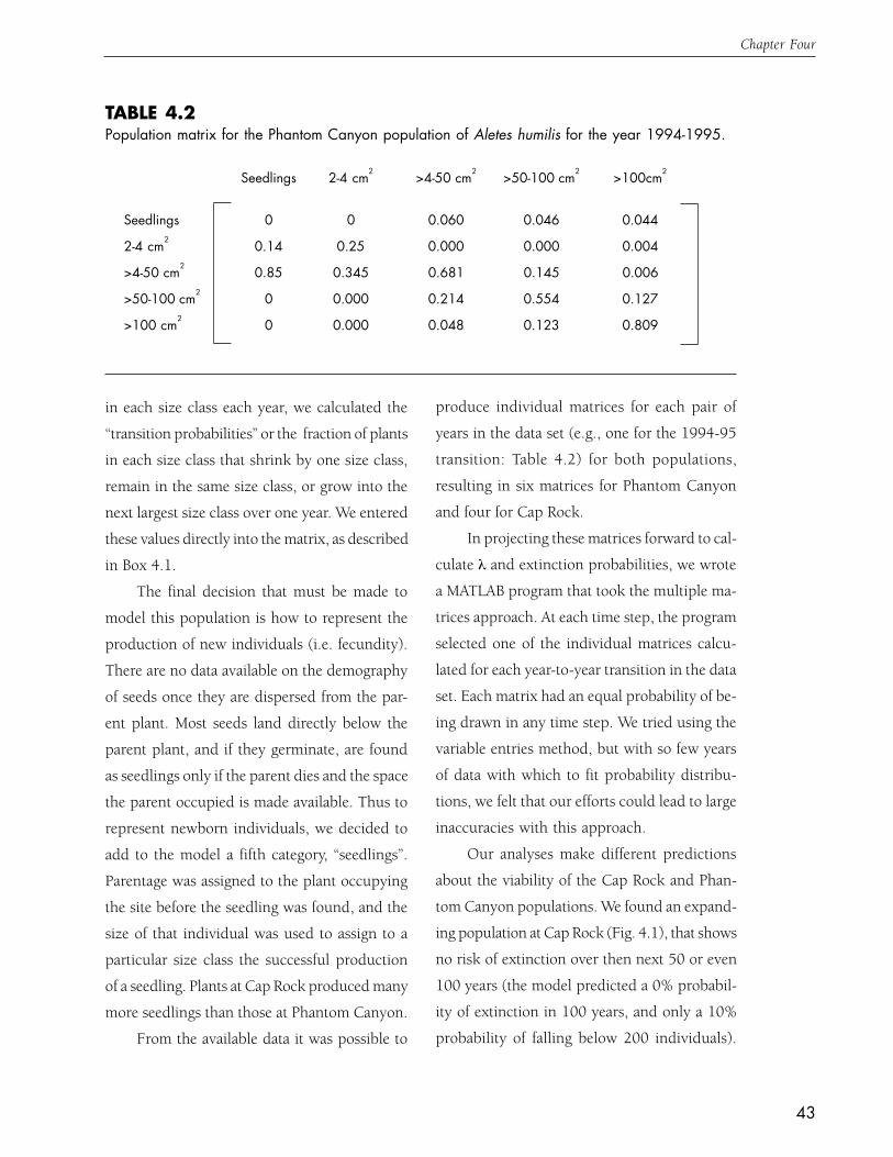
43

Chapter Four

in each size class each year, we calculated the

“transition probabilities” or the fraction of plants

in each size class that shrink by one size class,

remain in the same size class, or grow into the

next largest size class over one year. We entered

these values directly into the matrix, as described

in Box 4.1.

The final decision that must be made to

model this population is how to represent the

production of new individuals (i.e. fecundity).

There are no data available on the demography

of seeds once they are dispersed from the par-

ent plant. Most seeds land directly below the

parent plant, and if they germinate, are found

as seedlings only if the parent dies and the space

the parent occupied is made available. Thus to

represent newborn individuals, we decided to

add to the model a fifth category, “seedlings”.

Parentage was assigned to the plant occupying

the site before the seedling was found, and the

size of that individual was used to assign to a

particular size class the successful production

of a seedling. Plants at Cap Rock produced many

more seedlings than those at Phantom Canyon.

From the available data it was possible to

produce individual matrices for each pair of

years in the data set (e.g., one for the 1994-95

transition: Table 4.2) for both populations,

resulting in six matrices for Phantom Canyon

and four for Cap Rock.

In projecting these matrices forward to cal-

culate λ and extinction probabilities, we wrote

a MATLAB program that took the multiple ma-

trices approach. At each time step, the program

selected one of the individual matrices calcu-

lated for each year-to-year transition in the data

set. Each matrix had an equal probability of be-

ing drawn in any time step. We tried using the

variable entries method, but with so few years

of data with which to fit probability distribu-

tions, we felt that our efforts could lead to large

inaccuracies with this approach.

Our analyses make different predictions

about the viability of the Cap Rock and Phan-

tom Canyon populations. We found an expand-

ing population at Cap Rock (Fig. 4.1), that shows

no risk of extinction over then next 50 or even

100 years (the model predicted a 0% probabil-

ity of extinction in 100 years, and only a 10%

probability of falling below 200 individuals).

TABLE 4.2Population matrix for the Phantom Canyon population of Aletes humilis for the year 1994-1995.

Seedlings 2-4 cm2 >4-50 cm2 >50-100 cm2 >100cm2

Seedlings 0 0 0.060 0.046 0.044

2-4 cm2 0.14 0.25 0.000 0.000 0.004

>4-50 cm2 0.85 0.345 0.681 0.145 0.006

>50-100 cm2 0 0.000 0.214 0.554 0.127

>100 cm2 0 0.000 0.048 0.123 0.809

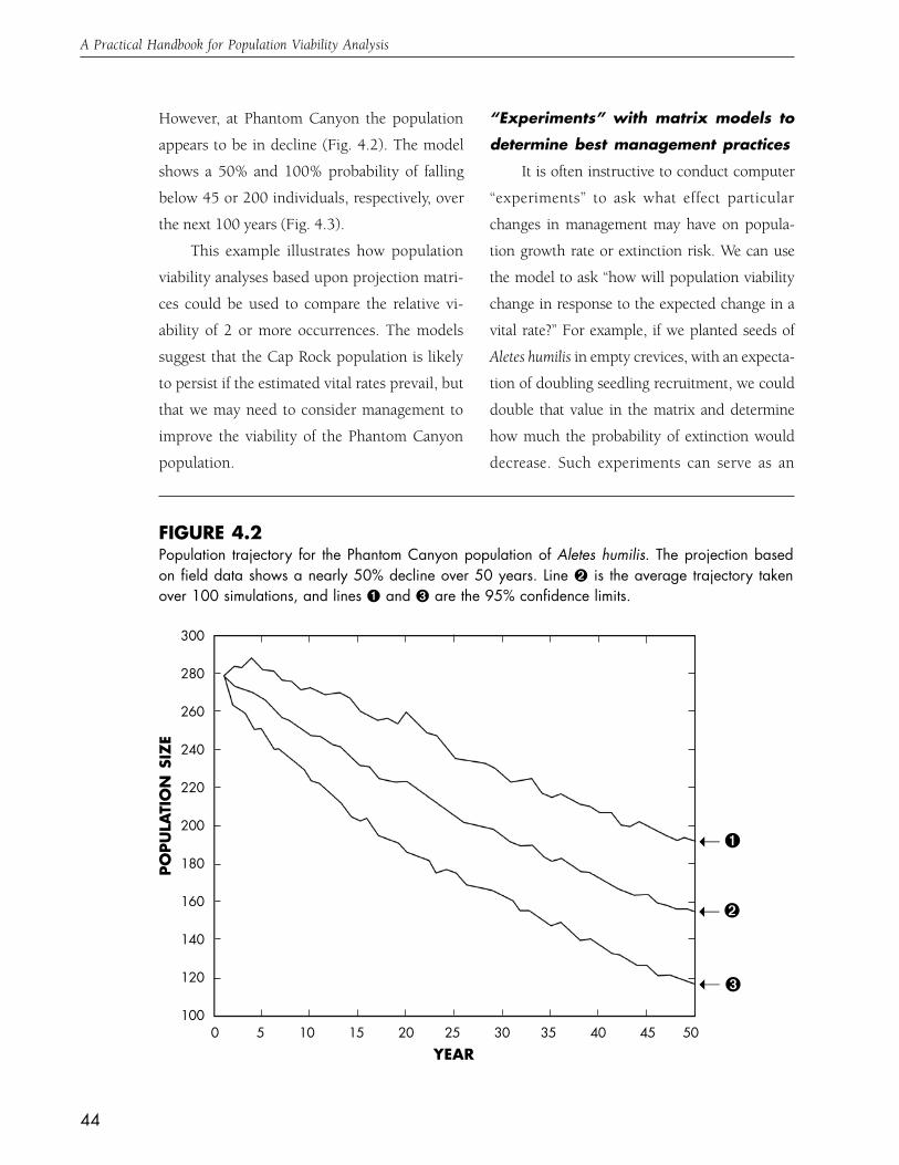
44


However, at Phantom Canyon the population

appears to be in decline (Fig. 4.2). The model

shows a 50% and 100% probability of falling

below 45 or 200 individuals, respectively, over

the next 100 years (Fig. 4.3).

This example illustrates how population

viability analyses based upon projection matri-

ces could be used to compare the relative vi-

ability of 2 or more occurrences. The models

suggest that the Cap Rock population is likely

to persist if the estimated vital rates prevail, but

that we may need to consider management to

improve the viability of the Phantom Canyon

population.

“Experiments” with matrix models to

determine best management practices

It is often instructive to conduct computer

“experiments” to ask what effect particular

changes in management may have on popula-

tion growth rate or extinction risk. We can use

the model to ask “how will population viability

change in response to the expected change in a

vital rate?” For example, if we planted seeds of

Aletes humilis in empty crevices, with an expecta-

tion of doubling seedling recruitment, we could

double that value in the matrix and determine

how much the probability of extinction would

decrease. Such experiments can serve as an

FIGURE 4.2Population trajectory for the Phantom Canyon population of Aletes humilis. The projection basedon field data shows a nearly 50% decline over 50 years. Line ➋ is the average trajectory takenover 100 simulations, and lines ➊ and ➌ are the 95% confidence limits.

300

280

260

240

220

200

180

160

140

120

1000 5 10 15 20 25 30 35 40 45 50

YEAR

POPU

LATI

ON

SIZ

E

➊

➋

➌

➝

➝

➝

45

Chapter Four

FIGURE 4.3Extinction risk profile for the Phantom Canyon population of Aletes humilis. The probability ofdropping below a threshold population size by 100 years is shown in the bold line, and the 95%confidence envelope is shown in the dotted lines.

0

0.2

0.4

0.6

0.8

1

0 50 100 150 200 250

EXTINCTION THRESHOLD

PRO

BABI

LITY

OF

EXTI

NCT

ION

indicator of the potential utility of specific man-

agement strategies. We can also ask the reverse

question: “in order to have an extinction risk

below 5% over 100 years (or an extinction risk of

100% over 5 years for an exotic we wish to

control), how large must a given matrix element

or elements be?” For example, we could deter-

mine how much greater seedling recruitment

would have to be to obtain a positive growth rate

for the Phantom Canyon population of Aletes

humilis, and then ask whether such a rate is prac-

tically achievable. Because recruitment is limited

by dispersal of seeds to sites not currently occu-

pied by adults, we asked whether doubling

seedling recruitment via seedling transplants

performed at various time intervals would be suf-

ficient to divert the population from its projected

decline. After several trials, we learned that only

if we planted seedlings every year would the

population begin to increase, although a few of

the simulation runs still decreased (see Fig. 4.4).

After performing additional analyses to be sure

of our result, and once sure that some interven-

tion is warranted, we could then assess whether

this type of intervention is feasible. This approach

can be extremely helpful for guiding manage-

ment decisions in many cases.

As we pointed out at the beginning of this

46


chapter, an informative use of matrix models is

to identify which life stage or which vital rates

have the greatest influence on overall population

growth. We can explore this question through a

series of computer “experiments” akin to the ones

we just described. The idea is to systematically

increase or decrease by a small amount each of

the elements in the matrix, one at a time, and

then examine the resulting rates of population

growth (for an example, see Crouse et al. 1987).

In this way we could ask, for example, whether

it is more effective to manage populations of A.

humilis by transplanting seedlings (i.e., enhancing

fecundities) or reducing trampling of established

plants (i.e., increasing survival of adults).

Finally, as our analysis of seedling trans-

plantation for A. humilis indicates, one can use

a matrix model to ask how frequently to apply a

management regime. For example, if we have

information on populations under two types of

management, say burned and unburned plots,

we could use a model to examine the effect of

different burning cycles on population growth

rates and thus determine the optimum burning

cycle (see Gross et al. 1998).

FIGURE 4.4A projection model “experiment” of doubling seedling recruitment via transplantation each yearshows the average population increases in size over 50 years (although some replicates stilldecline - see lower confidence limit). Line ➋ is the average trajectory taken over 100 simulations,and lines ➊ and ➌ are the 95% confidence limits.

900

800

700

600

500

400

300

200

100

0

0 5 10 15 20 25 30 35 40 45 50YEAR

POPU

LATI

ON

SIZ

E

➊

➋

➌

➝

➝

➝

47

Chapter Four

Prospects for the use of matrix-based

PVAs in TNC decision-making

Often, structured models are seen as im-

practical for application in TNC planning

efforts due to the amount of effort that must be

put into gathering sufficiently detailed data for

analysis. At a bare minimum, three years of

effort must be dedicated to marking, recaptur-

ing, and measuring individuals in a population

to even construct a stochastic matrix model.

However, three years of data would be insuffi-

cient to characterize the true degree of variation

in a population’s vital rates unless they are high-

ly invariant—put another way, the accuracy of

these models will depend on how well a few

years of data capture the range of variation the

population experiences. For most populations

many more years of data are required, especially

when evaluating populations subject to long-

term trends in vital rates or changes in manage-

ment practices. In this sense, projection matrix

models are likely to require as many years of data as

the count-based approaches, and of course much more

effort is required to gather these more detailed data.

Because of their data requirements, matrix-

based approaches will only rarely be of use in

ranking EOs.

Yet, while it is certainly true that it will not

be possible to perform projection matrix analy-

ses for very many species or locations, there are

cases in which this type of modeling will be more

informative and useful than less data-intensive

modeling efforts. Threatened and endangered

species of particular prominence, species with

large effects on ecosystems or on other species

(“keystone” species), indicator species, umbrella

species, or surrogates for a species of particular

concern are all likely candidates for this type of

PVA. When such species are long-lived, it will

be particularly valuable to adopt a matrix-based

approach to more accurately predict the popula-

tion consequences of changes in vital rates and

population structure. Results of matrix-based

PVAs for taxa of special interest may help us to

set goals for the size of particular reserves, or to

judge the overall effect of a management prac-

tice. The analysis of matrix projection models

can also help us to identify which life stages or

vital rates most influence population growth rate,

information that can be used to focus manage-

ment and monitoring efforts. Similarly, by using

the model to simulate different threats or by con-

trasting sites with different threats, it may be

possible to evaluate which threats are most

serious, and guide rescue efforts. Finally, because

it is possible to test probable outcomes of differ-

ent strategies by carrying out detailed “experi-

ments” with the model, matrix-based approaches

can serve an integral role in an adaptive context

of reserve management.

48

CHAPTER FIVEPopulation Viability for Multiple Occurrences,Metapopulations, and Landscapes

In Chapters 3 and 4, we considered the methods

available for estimating population viability of

single element occurrences, or single popu-

lations. Although the great majority of data

available to both TNC and other ecologists was

collected at only one site or population (Figure

2.1), many of the most pressing questions that

PVA should help to address involve multiple

occurrences. For example, how many popula-

tions are needed to ensure a high probability of

survival for a species? To what extent should

multiple occurrences be clumped versus spread

apart? Can small and low quality element occur-

rences add significantly to regional viability of a

species? Even among TNC’s most highly priori-

tized species, many occur in more than one—

or even more than five—sites (Figure 5.1); thus

the question of how best to protect species from

extinction nearly always involves the analysis

of populations arrayed across multiple sites with

particular spatial configurations. In this chapter,

we address the analysis of these complicated

situations.

Spatial population dynamics is an area of

ecology rife with highly complex models. In

particular, any conservation ecologist has prob-

ably read of the importance of “metapopulation

dynamics” for population viability and land-

scape-level planning (e.g., Gilpin and Hanski

1991, Hanski and Gilpin 1997, Doak and Mills

1994, McCullough 1996). However, the data

available for most species of concern do not

include enough or the right kinds of information

to justify these complicated modeling methods.

For example, the data sets (see Fig. 2.1) sub-

mitted to the PVA workshop from which this

handbook grew were completely devoid of

information on dispersal rates or distances or

even the spatial locations of individuals. There-

fore, even more than in previous chapters, we

will take an approach here that distinguishes

useful methods for viability assessment in the

face of realistic data limitations from more

ideal analyses that simply require too much

information.

Data limitations are typically so severe for

multiple site viability analyses that the word

“analysis” is itself a little misleading. Often,

when examining questions about multiple

occurrences the best we can do is a structured

form of thought experiment. It would be easy to

read this chapter and conclude that there will

never be enough data to rigorously perform

viability analysis for multiple occurrences.

However, data scarcity does not mean that we

need to be paralyzed. Using the approaches

we discuss below can often illuminate non-

obvious tradeoffs or important questions that

can improve viability planning. While the lack

of data to perform multiple occurrence viability

49

Chapter Five

0

50

100

150

200

250

300

350

400

1 4 7 10 13 16 19 22 25 28 31 34 37 40s 70s 100s 130s 160s 190sNUMBER OF OCCURRENCES

NU

MBER

OF

SPEC

IES

Number of G1 Species

Number of G2 Species

single groups groups of tens

FIGURE 5.1Number of known occurrences for TNC priority G1 and G2 species. Histograms show the numberof occurrences per species, grouped for single numbers of occurrences below 40 occurrences,and in groups of ten (e.g., 50-59 occurrences) above 40.

analysis correctly is a constant frustration, ex-

ploring the options using some fashion of

quantitative reasoning can be highly useful.

We will begin by discussing the types of

information that are ideally available to analyze

the viability of multiple populations, then pro-

gress from simple to more complex methods of

analysis. Finally, at the end of the chapter we

will offer some general guidelines for multi-site

considerations that should play a role in con-

servation planning.

Data Needed to Understand Multiple

Sites and Populations

The primary reason that viability assessment

for multiple sites is more complicated than single-

site PVA is the need for more and different data.

In particular, there are three distinct classes of

data that are relevant for multiple site planning.

Only very rarely will all three types of data be

available for a given species. However, before

diving into how to proceed without this infor-

mation, it is important to clarify what is needed

for a full analysis, and why:

The quality of each population being con-

sidered. Essentially, ‘quality’ here means the

results of a single site PVA, as discussed in Chap-

ters 3 and 4. While there can be many aspects

to an assessment of population quality (see Box

5.1), the most useful result for linking together

multiple site analyses into a multiple occurrence

PVA is some estimate of the probability of pop-

ulation persistence at each site over some clear

time horizon.

Correlations of the fates of populations due

to shared environments. The most important

influence of spatial arrangement on overall via-

bility is the extent to which (continued on page 51)

50


BOX 5.1 (Key): Methods of AnalysisMethods to Judge Single Site Quality

Ideally, when judging the importance of a site for a multi-occurrence viability plan, we would have the resultsfrom analyses like those presented in Chapters 3 and 4 for each and every site. In particular, using either themethods of Dennis et al. (1991), or stochastic simulations of projection matrix models, we would like tohave an estimate of extinction probability (over some specified time horizon) for each population. However,even if we have good enough data from one population to perform such an analysis, we usually don’t havesufficient information to do any analysis for most populations. This leaves three common choices:

1. The “Representative Sites” Method. Use data from one or two well-studied sites to makequantitative estimates of viability for other occurrences (see Fig. 3.7B and Box 5.2). While this is usually themost reliable way to proceed, we still have to be somewhat skeptical of these estimates, since the genetics andthe environmental conditions (both natural and anthropogenic) that together control the demography ofeach population is unlikely to be identical. Nonetheless, such estimates provide a good starting point formultiple occurrence viability planning.

2. Wild (or Educated) Guesses. Without any good data on any population of our species, wemust resort to guessing about the likelihood of extinction. These guesses can take many forms: a) modificationsof quantitative viability estimates using data from other, related species; b) historical data on estimatedpopulation sizes and rates of extinction of a formerly common species (e.g., Berger 1990); c) natural historyintuition and broad patterns of viability. This last method is essentially using any available information to putbrackets around extinction probabilities and the way that they are likely to vary with population sizes.Familiarity with a taxonomic group and the work that has already been done on other species within thetaxon can yield valuable information upon which to build viability estimates. For example, Heppell (1998)has summarized work on multiple turtle species to arrive at generalizations about the demographic patternsof this group. The key strategy in using this “anything goes” approach is to avoid making singleestimates of extinction rates. Rather the focus should be on making minimum and maximum estimatesthat bracket reality. We can often make such estimates even when we can’t know the specifics of a population’schances of survival. Using both the minimum and maximum estimates in our calculations then gives us arange that, to the best of the available knowledge, bounds the likely viability. Surprisingly frequently, thepractical answers for a conservation strategy do not require more than these “brackets.”

One further point that should receive special attention here is the need to consider changing conditionsin estimating single site quality or viability. Even if all the data needed for the Dennis et al. approach are inhand, the effects of future management (to improve a population’s probabilities of survival) or future impacts(which may greatly reduce the chances of survival) should be weighed in making population viability estimates.

3. Despair. We do not encourage this approach. Although analyzing multiple occurrence viability isnot simple, and we are always limited by the data at hand, it is much more profitable to go through the stepsof a simple analysis with guesses than to not do it at all. Partly, this is because of the initially non-intuitiveanswers that often emerge from viability analysis (often ‘non-intuitive’ results become intuitive once they arereflected on). Partly, analysis is useful because it can clarify the need for some kinds of information and theunimportance of other information. One of the most useful outcomes of models in conservation is thesetting of priorities for information we need to gather.

51

Chapter Five

populations at different sites will share the same

fate at the same time. Thus, if two populations

are in close proximity, they are likely to be similarly

affected by variations in the environment, whether

these variations are “normal” vacillations in

rainfall, or “extreme” events such as fires and hur-

ricanes. Other factors, such as elevation on a flood

plain, can also generate correlations that are

unrelated to simple physical proximity. There are

many different ways—in theory—to estimate and

measure the degree of correlation in the fates of

populations. However, there are currently few

good general methods with which to carry out

such analyses, and we rarely have the data needed

to use these rigorous estimation techniques. Only

for the simplest types of catastrophes is it an easy

matter to estimate correlations in the probabilities

of extinction of two occurrences. However, using

correlations in weather fluctuations, knowledge

of the sizes of major disturbance events, and other

less precise estimates of how much or how little

each pair of sites will be correlated can still be

highly informative, as we discuss below.

How much movement occurs between each

pair of populations? Estimation of movement

rates is important for several reasons, including

the genetic effects of movement, the potential

of spatially separated populations to ‘rescue’ each

other from extinction (in the ‘rescue effect’,

dispersers from other populations add numbers

to a failing population and therefore rescue it

from extinction), and the possibility that a

population that goes completely extinct might

be recolonized through immigration. While there

are many methods available to estimate move-

ment rates for different taxonomic groups

(Turchin 1998), most are complex and are often

extremely labor-intensive. As we discuss in the

next section, the most important questions con-

cerning movement of a target species may often

be fairly easily answered with good knowledge

of the basic natural history.

A Schematic Breakdown of Multiple

Occurrence Scenarios.

Using a qualitative description of different

degrees of movement and different correlations

in the fates of populations, we can distinguish

several distinct conservation scenarios (Table

5.1), each of which require somewhat different

approaches to viability analysis.

High correlation in the fates of different

populations (Cases A1, A2, A3): spatial analysis

not required. When there is a high correlation

in the fates of different populations, then there is

little need to enter into the quagmire of spatial

population analysis. It is easiest to understand

this point by realizing that correlations of popu-

lation-level fates are generated by correlations in

the fates of individuals. The highest degree of

population-level correlation that is likely to occur

is when two individuals in separate populations

are no less correlated in their fates than are two

individuals that are in the same population. For

example, if essentially all the temporal variation

in the environment is generated by large scale

weather events (e.g., hurricanes or El Niño

events), then individuals in populations sepa-

rated even by dozens of kilometers may be thought

of (more or less) as members of a single popula-

tion, at least in terms of how their fates affect the

risk of species extinction. In this circumstance,

52


TABLE 5.1Six combinations of movement rates and correlations in fates are likely to actually occur. If move-ment rates are high between two populations, it is difficult for their fates to be less than highlycorrelated, thus two of the cells will never occur. In addition, low to medium movement is expectedto cause at least some interpopulation correlation, so one cell is unlikely to occur. We also includeexamples of species that appear to exemplify each combination; for these examples, we havepicked relatively well-known species and made judgement calls about the correlation categoriesinto which each would fit. In most of these cases, data that would allow the correlations to becalculated are lacking.

Correlation inPopulation

Fates

Movement BetweenPopulations

NONE

LOW TOMEDIUM

HIGH

NONELOW TOMEDIUM HIGH

Case BPlants on scattered

Chicago prairiefragments (Panzer

and Schwartz 1998)

Case CEndemic annuals onscattered serpentine

outcrops inCalifornia

(Kruckeberg 1984)

Birds in San Diegochapparal fragments(Bolger et al. 1991)

Case A1Insects in scattered

Chicago prairiefragments (Panzer

and Schwarz 1998)

Unlikely to exist Can’t exist

Can’t exist

Case DFurbish’s Lousewort

in Maine (Menges1990)

Case A2Bay Checkerspot

Butterflies (Harrison1989)

Case A3Acorn woodpeckersin Southwest (Stacey

and Taper 1992)

there is probably little benefit from having

multiple populations other than a simple increase

in the total number of living individuals and

possible increases in local genetic diversity. Thus,

the methods described above for single popula-

tions are all we need to adequately assess viability.

Obviously, Cases A1, A2, and A3 do differ from

one another, ranging from what is in fact a single

intermating population (A3) to what are utterly

distinct populations (A1). However, the key point

is that for all these situations, we can avoid the

complications of spatial population analysis and

still do a good viability assessment.

Isolated, independent populations. When

there is effectively no movement between popu-

lations and there is little or no correlation in

53

Chapter Five

the fates of populations (Case B), then the

advantages of protecting multiple populations

can be extremely large. Each population repre-

sents an independent chance of continued

existence and the probability of global extinction

will decline rapidly with the number of occur-

rences. Even better, the methods of analysis for

this situation include some simple extensions

of the approach presented in Chapter 3. The

crucial question is how to determine the overall

probability of extinction, over some time horizon,

for a collection of independent populations

(occurrences). Or, stated as the decision that

must frequently be made: given that some popu-

lations of a species are already preserved, what

will be gained by preserving additional popula-

tions? The method used to assess this question

relies upon the independence of the fates of

each population. Given this independence, the

probability of all M populations becoming

extinct is simply the product of the probabilities

that each individual population in the collection

becomes extinct:

Equation 5.1

Pglobal

= P1

* P

2 * P

3 *

P

4 *

P

5 * ... * P

M

where Pi is the probability that population i

becomes extinct over some fixed time horizon,

and where Pglobal

is the probability that all M

populations die out.

Using this simple formula, one can easily

understand the assertions by various authors that

preserving three or four populations will usually

be enough to ensure a good chance of viability

(Figure 5.2, Pi = 0.2 or 0.4). We can also see why

these generalizations should not be taken too

FIGURE 5.2Changing risk of extinction with increasing numbers of populations. These probabilities are calcu-lated using equation 5.1, assuming that extinction risk is uncorrelated and that all populations havethe same probability of extinction, Pi. Each line shows changing risk of total extinction, as a function ofthe number of populations, for a different per-population extinction probability.

0.0

0.1

0.2

0.3

0.4

0.5

0.6

0 5 10 15 20NUMBER OF OCCURRENCES

PRO

BABI

LITY

OF

TOTA

L EX

TIN

CTIO

N

Pi = 0.60

0.40

0.20

54


seriously (Figure 5.2, Pi = 0.6); while there is often

a dramatic effect of adding additional populations

on the safety of the whole set of occurrences, exactly

how much additional safety is generated depends

critically on the individual extinction probabili-

ties of each occurrence. For example, adding many

poor-quality (i.e., extinction-prone) populations

to a set of occurrences already including two high-

quality populations may have little effect on overall

safety. In contrast, if all populations are relatively

extinction prone, then there can be a substantial

gain in safety from increasing numbers of occur-

rences (Figure 5.2, Pi = 0.6). Perhaps the most

important message from this type of analysis is

that the importance of different population occur-

rences for overall viability is highly dependent upon

the quality of all sites. That is, there is no clear

cut-off of single-population extinction probabil-

ity below which a population can simply be dis-

missed as unimportant. In Box 5.2, we show how

to use this method to assess the overall viability

of the set of isolated grizzly bear populations

inhabiting the Lower 48 United States and British

Columbia.

Clearly, situations in which there is no migra-

tion and no correlation in the factors affecting a

set of populations are extremely unlikely. How-

ever, even when we know—but do not have data

to quantify—that some inter-population movement

and some correlation in fate exists, this simple

approach is usually worth taking, simply because

it gives a good starting point for analyzing the

relative merits of protecting multiple sites. Further-

more, the results of this analysis can give much

more meaning to our qualitative understanding

of movement and correlation. If there is some

correlation of population fates, but little or no

movement, then the added safety of multiple

protected sites will be weakened. Conversely, if

there is some movement between sites, but little

correlation in the effects of catastrophes on different

populations, then there is likely to be more safety

in numbers than the simple analysis shows. Having

a clear, quantified bench-mark against which to

set these statements of ‘more or less safety’ gives

them far more meaning and importance. We now

turn to methods with which to analyze these

complications directly.

No inter-population movement, but mod-

erate correlation in fates of populations. When

there is no direct interaction of populations (i.e.,

no movement of individuals between populations),

but there are common factors influencing the

growth, decline and extinction of separate popula-

tions, the safety gained by preservation of multiple

sites can be substantially degraded (Case C). In

theory, quantifying the gain in probability of overall

extinction with correlated fates is a very simple

extension of the last case. We modify equation 5.1

slightly to read:

Equation 5.2

Pglobal

= P1 * P

(2|1) * P

(3|1,2) *…..* P

(M|1,2,…,[M-1])

where P(i|1,2,…,[i-1])

is a conditional probability; in

words, it is the probability that population i goes

extinct given that populations 1 through i-1

already have or will simultaneously become ex-

tinct. The insertion of these conditional proba-

bilities is a way of incorporating correlated risk

into the formula. For example, if the probability

of extinction over 100 years is 0.2 for each of

two populations, then the (continued on page 57)

55

Chapter Five

BOX 5.2 (Key): Methods of AnalysisAnalysis of Multiple Occurrence Viability for the Grizzly Bear

While we did not find a data set from TNC that would clearly (and cleanly) serve as an illustrativeexample for multiple occurrence viability assessment, many such data sets do exist. Here, we use theresults for the Yellowstone grizzly first described in Chapter 3 to show how such an assessment can bedone. It is worth emphasizing at the outset that this question is not an abstract one; ongoing planningand litigation concerns the question of the overall viability of the small and scattered grizzly populationsin the Lower 48 United States.

There are five known grizzly populations in the Lower 48 United States and adjacent parts ofCanada, with minimum estimated population sizes ranging from 306 in the Northern ContinentalDivide Ecosystem to five in the North Cascades (United States Fish and Wildlife Service 1993; Table5.2). Since each of these areas is distinct and fairly isolated from the others, we will proceed with ananalysis that assumes both that there is no movement between the populations (which is almost certainlytrue) and that there is no correlation in the fates of the populations. This second assumption is notcorrect; there is good evidence of widespread environmental factors, including weather and masting ofwhite-bark pines (Mattson et al. 1992), that will create at least some correlations in the fates of bearpopulations in the inter-mountain West. However, since we cannot clearly evaluate the strength of suchcorrelations, we will proceed here with the simplifying assumption of totally independent fates. Wediscuss the issues of correlated fates in more detail in the body of the chapter.

To estimate the viability of each population, we used the Dennis et al. method described in Chapter3. Since not all of the five grizzly populationshave enough data to estimate µ and σ2, weinstead use estimates from the very extensiveYellowstone data set (Dennis et al. 1991; µ =-0.007493 and σ2 = 0.008919). Using thesevalues, we calculated the probability of ex-tinction at 500 years, assuming an extinctionthreshold of 2 bears (Table 5.2; for methods,see Box 3.3).

Given our estimates of single populationviability, we can ask a variety of questions aboutthe advantages for overall viability of protectingdifferent combinations of the five populations.First, what are the gains of adding sequentiallysmaller populations to a collection of occur-rences for this species? For the 500 year timespan, protecting the Yellowstone population inaddition to that of the Northern Divide decreasesthe probability of extinction from 0.342 (forthe Northern Divide alone) to the product ofthe two populations’ extinction probabilities:0.342*0.392 = 0.134. (continued on page 56)

TABLE 5.2Single population viability estimates for fivegrizzly populations. *Current size is a minimumestimate of current population size. Data fromUnited States Fish and Wildlife Service 1993.

PopulationCurrentSize*

Probability ofExtinction

(500 years)

NorthernDivide

Yellowstone

Selkirks

Cabinet/Yaak

NorthCascades

306

236

25

15

5

0.342

0.392

0.823

0.890

0.974

56


BOX 5.2 (continued)

While this dramatic gain in safety may not seem surprising, there is also a substantial lessening of extinctionrisk from adding the much smaller Selkirk population to the first two: 0.342*0.392*0.823= 0.110.Figure 5.3 illustrates that adding the remaining two populations to the portfolio of sites yields diminishingbenefits.

Another question is whether the three smallest populations together can guarantee as little risk ofextinction as either of the two largest populations. The answer is no: the three small areas together havea combined extinction risk about double that of either of the two larger populations alone:0.892*0.890*0.974 = 0.713. However, in terms of bears alive at the present time, this is a surprisinglysmall extinction risk, since these three populations together harbor only 45 individuals, less than a fifththe number in either of the two large populations.

Finally, one way to view the results of this type of analysis is simply to ask about the safety fromregional extinction under the very best scenario of maintenance of all current populations. For 500years, we would predict only a 9.6% chance of extinction of all populations (100*0.342*0.392*0.823*0.890*0.974). While reasonably small, this risk is still greater than the 1% chance of extinctionover reasonable time horizons that is frequently called for in conservation. Worse, we know that it iscertainly a low estimate, since the two largest populations are relatively close together and thus willshare correlated fates. By showing that our optimistically simple analyses yield inadequate safety, ananalysis like this one can support the need for more proactive conservation measures.

FIGURE 5.3Extinction risk for sets of grizzly bear populations over 500 years. From left to right, each barplots the global extinction probability obtained by adding sequentially smaller populationsto a collection of protected areas.

0

0.05

0.1

0.15

0.2

0.25

0.3

0.35

0.4

just N

othern

Divi

de

and Y

ellow

stone

and S

elkirk

s

and C

abine

t/Yaa

k

All pop

ulatio

ns

EXTI

NCT

ION

RIS

K

57

Chapter Five

probability that both become extinct indepen-

dently is 0.04. However, if extinctions are highly

correlated—perhaps due to fires that might spread

through both populations—then the risk of

extinction of the second population might be 0.8

if the first population becomes extinct. Therefore,

the overall risk of extinction is 0.2*0.8 = 0.16. In

this case, the gain in safety (= reduction in risk

of extinction) that is realized by preserving two

versus one population is much more modest.

Adding correlation can strikingly reduce the

effectiveness of multiple occurrences in creating

safety (Figure 5.4). However, the extent to which

correlations counteract the gains from multiple

protected sites depends on the details of each

situation. In particular, it is unlikely that all

populations are equally correlated in their fates.

Especially if physical proximity results in high

correlation, it may be beneficial to preserve sites

that are as distant as possible from one another.

In other words, when movement either doesn’ t

occur, or is of relatively little importance, the risks

that proximity poses by increasing correlated

extinctions is of paramount importance and should

be minimized. While this advice runs counter to

standard conservation recommendations, the

reasoning is straightforward and likely to be as or

more important than the considerations of move-

ment between populations that underlie recom-

mendations to place reserves close together (see

next section).

How can we apply this abstract reasoning

to real situations (that is, how do we estimate

the conditional probabilities in equation 5.2)?

Analysis of the extent to which conservation gains

are eroded by correlations can either be quite

complicated or fairly simple. As usual, the tract-

able case, with which we will start, is less realistic.

The key assumption in making a correlated ex-

tinction problem simple is that the major factors

causing population extinctions are discrete ‘catas-

trophes’ that can strike more than one population

at a time: fires, floods, epidemics, and droughts

are among the likely factors causing such cor-

related extinctions. In this case, we simply need

to know the probability of each population suc-

cumbing to extinction given that others have or

will also become extinct. This type of data is rarely

available from real extinction records. However,

physical data such as records of fire sizes and

correlations in rare weather conditions across the

range of populations can provide good guidelines

for estimating the correlations in extinction risks

from such discrete events.

A more complicated situation arises when

factors other than catastrophes drive extinctions.

In particular, “normal” environmental fluctuations,

as discussed in Chapter 3, can result in extinctions

that are driven by series of poor, but not catas-

trophic, years. In this case, shared environments

still can drive correlated extinctions, but it is much

more difficult to estimate the correlations, because

they are the result of shared events over many

years. There are as yet no clear analytical results

that are comparable to those of Dennis et al. (1991)

with which to analyze this situation. However,

computer simulations of multiple populations

reacting to correlated environmental fluctuations

can be used to untangle correlations in extinction

probabilities (Harrison and Quinn 1989); to apply

these methods to a real situation will probably

require collaboration with a (continued on page 59)

58


FIGURE 5.4The safety of multiple occurrences given correlation in extinction rates. The probability of extinctionover all populations is plotted versus the number of patches, for no correlation (open circles) andlow (open squares), medium (filled diamonds) and high correlation (crosses). The probability thata single patch becomes extinct is 0.1 for all lines. Note that there is no single best way to addcorrelation in extinction rates; the degree of correlation and its pattern are outcomes of the biologi-cal and physical forces that cause extinction in each situation. For this example, we have used asimple functional form to add correlation in extinction risk*. However the pattern shown in thefigure is very general; it doesn’t depend upon the exact function used.

* In making this figure, we have assumed that the probability of extinction for a patch increases ifother patches have already gone extinct. We estimate the extinction probability of M patches as:

Pglobal

= (1 – P1)

1 + a (n – 1)b1 –Π

M

n=1

(see equation 5.2)

Here, P1 is the probability that a single, isolated patch becomes extinct. The parameter a controls theoverall strength of correlation, while b is a shape parameter, affecting the pattern of correlations (i.e.,if more and more patches suffer extinction, is there a diminishing, linear, or accelerating influence onthe extinction probabilities of remaining populations?). In this figure, we have assumed that b = 1 forall lines, while a = 0 for no correlation, and 0.05, 0.2 and 1 for low, medium, and high correlation,respectively.

0

0.02

0.04

0.06

0.08

0.1

0.12

1 2 3 4 5 6 7 8 9 10 11 12 13 14 15 16 17 18 19 20

NUMBER OF OCCURRENCES

PRO

BABI

LITY

OF

TOTA

L EX

TIN

CTIO

N

59

Chapter Five

modeler who can tailor a simulation to the specifics

of a real system.

Movement, although not extensive, is impor-

tant, and populations are not highly correlated

in fates. Here we finally come to the situation

that is usually the only one presented in dis-

cussions of multiple populations and conser-

vation strategies: simple metapopulations (Case

D; see Box 5.3 for a run-down on basic meta-

population ideas applicable to TNC problems).

In this situation, multiple occurrences provide

greater safety for the same reasons discussed above

under Cases B and C, but there is also potentially

a huge additional gain in safety from movement

between populations. Movement can either result

in recolonization of habitat patches in which pop-

ulations have gone extinct, or prevent extinctions

through ‘the rescue effect’.

Before now we have dismissed movement,

in spite of its potentially huge importance in

determining the safety of multiple occurrences,

simply because of the difficulty in acquiring good

data on dispersal. Since we must usually make

wild guesses at movement rates, our philosophy

is that it is often better—at least initially—to

pretend that it doesn’t happen. This will give us

both more conservative estimates, and also esti-

mates that do not rely upon very suspect guesses.

However, it is still worthwhile to consider meta-

population processes and their implications for

multiple occurrence analysis, both because in

some circumstances movement is relatively well-

understood and important (Beier 1993) and be-

cause these ideas are so prevalent in the conser-

vation literature.

In the simplest metapopulation situation, two

processes counter one another: the extinction of

local populations, and the recolonization of habitat

patches. For this simple situation, the mean time

to extinction depends upon four variables: the

probability of local patch extinction, the rate of

movement between patches, the number of habitat

patches (not all of them occupied all the time),

and the correlation in extinction probabilities

(Figure 5.5). Each of these factors has the effect

that one would expect, with the best possible

combination being that: 1) there is low probability

that each local population becomes extinct; 2)

rates of movement between populations are high;

3) the number of habitat patches is large; and 4)

extinction of different populations is uncorrelated.

In the extreme, these conditions mean that we

don’t have to consider a collection of populations

as a ‘metapopulation’ at all (Table 5.1). However,

as we have mentioned above, there is an important

complication that is ignored in most treatments

of simple metapopulation theory, the confounding

of correlation in local population fate (extinction

times) and movement rates. For almost all species

and patch arrangements, there is likely to be a

strong effect of the distance between patches on

both movement rates and the shared chance of

extinction. Thus, greater proximity will result in

the opposing effects of higher movement rates and

greater correlation in extinction, with an uncertain

net outcome for global extinction risk.

Even incorporating the complications just

mentioned, most metapopulation models are

far too simplified for on-the-ground conserva-

tion planning. In particular, they rely on assump-

tions of equal immigration rates between all habi-

tat patches, as well as equal (continued on page 62)

60


Equation 5.3

BOX 5.3 (Key): Theoretical UnderpinningsThe Basics of Metapopulations

While a great deal has been written about metapopulation dynamics (Levins 1969, Gilpin and Hanski1991, Hanksi and Gilpin 1991, 1997), it is worthwhile here to provide a quick review of basicmetapopulation models. In part this is because most of the general statements about conservation ofmultiple occurrences come directly from the simplest metapopulation models, and in part becausemost of the more elaborate models are built directly on the framework of Levins’ original ideas.

In large part, the influence of the original metapopulation model (Levins 1969) comes from itssimplicity. In this model, only two parameters are assumed to control the metapopulation: the rate atwhich occupied habitat patches become extinct (e) and the rate of recolonization, or founding ofpopulations on unoccupied habitat patches (m). Most simply, the measure of the metapopulation’s sizeor health is the proportion of suitable habitat patches with an extant population (p). Thus, p rangesfrom 0 to 1 (i.e., from no patches occupied to all occupied). The change in this proportion is a functionof e and m:

Several assumptions are implicit in this model. First, it is assumed that colonization arises solely due toimmigration from currently occupied patches in the metapopulation (i.e., not from populations outsidethe metapopulation being considered). Thus, m is the rate at which colonists from extant patches findand successfully colonize empty patches, and mp(1–p) is the overall rate of colonization, given p.Furthermore, this model assumes that all patches are equally likely to provide colonists to any otherpatch. This is equivalent to assuming that all patches are equally far apart and that they are all of thesame size and quality. The loss of populations due to extinction is represented by –ep. Thus, e is asimple rate of local population extinction, and there is again the implicit assumption that all populationsare identical—that they all share the same probability of extinction per unit time—as well as that theseextinction probabilities are completely uncorrelated with one another. Finally, Levins’ model does notinclude rescue effects; each population’s probability of extinction is independent of how many otherhabitat patches are occupied. For clear but more detailed reviews of this model and its basic modifications,see Gotelli (1991, 1995).

One crucial point to make is that, as presented above, simple metapopulation models do notinclude any explicit term for the number of habitat patches that might support populations. Indeed,the theory relies on the assumption that there are enough patches that we can summarize averagebehavior using just the proportion of occupied patches. However, to make any useful predictions forrare species, with finite numbers of populations and habitat areas, we need to explicitly include thenumber of patches in our model. Nisbet and Gurney (1982) have produced such a model, allowingthe estimation TM , the mean time to extinction for a metapopulation with a total of H patches:

dp

dt= mp(1 – p) – ep

TM = TL expH

2(mTL +

mTL

1– 2)

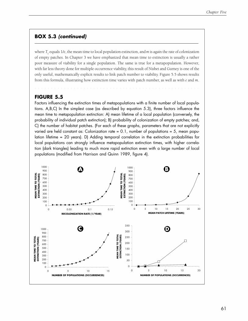
61

Chapter Five

BOX 5.3 (continued)

FIGURE 5.5Factors influencing the extinction times of metapopulations with a finite number of local popula-tions. A,B,C) In the simplest case (as described by equation 5.3), three factors influence themean time to metapopulation extinction: A) mean lifetime of a local population (conversely, theprobability of individual patch extinction); B) probability of colonization of empty patches; and,C) the number of habitat patches. (For each of these graphs, parameters that are not explicitlyvaried are held constant as: Colonization rate = 0.1, number of populations = 5, mean popu-lation lifetime = 20 years). D) Adding temporal correlation in the extinction probabilities forlocal populations can strongly influence metapopulation extinction times, with higher correla-tion (dark triangles) leading to much more rapid extinction even with a large number of localpopulations (modified from Harrison and Quinn 1989, figure 4).

0100

200300

400500600

700800

9001000

0 0.05 0.1 0.15

RECOLONIZATION RATE (1/YEAR)

MEA

N T

IME

TO T

OTA

L EX

TIN

CTIO

N (

YEA

RS)

0100200300400500600700800900

1000

0 5 10 15 20 25 30

MEAN PATCH LIFETIME (YEARS)

MEA

N T

IME

TO T

OTA

L EX

TIN

CTIO

N (

YEA

RS)

0

100200

300400

500600700800900

1000

0 5 10 15

NUMBER OF POPULATIONS (OCCURRENCES)

MEA

N T

IME

TO T

OTA

L EX

TIN

CTIO

N (Y

EARS

)

0

50

100

150

200

250

300

350

0 5 10 15 20

NUMBER OF POPULATIONS (OCCURRENCES)

MEA

N T

IME

TO T

OTA

L

EXTI

NCT

ION

(Y

EAR

S)

A

where TL equals 1/e, the mean time to local population extinction, and m is again the rate of colonizationof empty patches. In Chapter 3 we have emphasized that mean time to extinction is usually a ratherpoor measure of viability for a single population. The same is true for a metapopulation. However,with far less theory done for multiple occurrence viability, this result of Nisbet and Gurney is one of theonly useful, mathematically explicit results to link patch number to viability. Figure 5.5 shows resultsfrom this formula, illustrating how extinction time varies with patch number, as well as with e and m.

B

C D

62


population sizes and extinction risks in all habitat

patches. To tailor these scenarios to specific prob-

lems and decisions requires more elaborate simu-

lation models that take these basic ideas and

apply them to more complicated situations. While

these highly specific simulations are beyond the

scope of this handbook, in Box 5.4 we outline

three basic approaches to such an analysis. Unfor-

tunately, only rarely will there be enough data

available to perform such simulations with any

confidence.

As we’ve repeatedly stated, the information

needed to address Case D in our table of spatial

situations is rarely available or obtainable without

extended, intensive sampling. However, this is

not to say that ‘metapopulation-like’ spatial situa-

tions are uncommon or unimportant. This leaves

the obvious conundrum of how to analyze multi-

site viability with the usual mismatch between

conservation needs and data availability. In

the final section of this chapter we provide some

thoughts on approaches to this problem.

Assessing Multi-population Viability

with Realistic Constraints

The basic problem in assessing multi-

population viability is the need for three distinct

types of information: everything needed to assess

single population viability, movement rates

between populations, and correlation in the

factors influencing different populations. Without

all this information, we are left with the question

of how to actually proceed without knowing where

in Table 5.1 we really are. We suggest the follow-

ing way of approaching this all-too-typical set of

limitations:

1. First, reclassify all occurrences of a species

into sets. Each set should include sites that are

likely to have enough movement and/or correla-

tion in environments that they are best considered

as one population unit for viability analysis (note

that these groups of occurrences might be distant

enough from one another spatially that they should

certainly be considered as separate EOs in stan-

dard TNC protocols). However, different sets

should be defined so that they are likely to be

relatively independent population units.

2. Treat each set of highly correlated EOs as

a single, unified population, estimating its viabi-

lity using single-population methods. Then per-

form the simplest type of multi-population viabi-

lity assessment (equation 1) on the sets rather than

their component populations, assuming that no

movement or correlation occurs between sets. While

this type of analysis is clearly over-simplified, it

provides a starting point from which to guess at the

importance of movement and correlation effects.

3. Use this simplest analysis to make initial

guesses at the effects of keeping or removing

different populations. However, do not accept

these results as a final answer, but rather as a

starting point, to which can be added further

knowledge of the species’ natural history. For

example, while this type of analysis might sug-

gest that a small population close to several others

is unimportant, such habitat patches might be

of known importance for the enhancement of

movement between other populations, and this

qualitative knowledge should be used to modify

the conclusions of the formal viability assessment.

4. Finally, in using this type of simplified ana-

lysis to frame a preservation (continued on page 64)

63

Chapter Five

BOX 5.4 (Optional): Methods of AnalysisMethods for Quantitative Analysis of Complicated MultipleOccurrence Situations

Three general approaches have been developed to deal with the complications of multiple occurrencepatterns. While all have limitations, each adds reality to the bare-bones assumptions of the simplestmetapopulation models reviewed in Box 5.3. Below, we simply provide a thumbnail sketch of eachapproach, along with references for further reading.

More complicated metapopulation approaches. Numerous papers have been published thatdirectly elaborate on the basic Levins metapopulation model. Perhaps the most promising of theseapproaches is the “incidence function” method of Hanski (Hanski 1991, Hanski et al. 1996). Theessential idea of this approach is to use data that are relatively easy to collect for separate populations toestimate the more difficult to obtain extinction and colonization rates needed for a metapopulationmodel. These models add reality to the metapopulation approach by estimating how extinction andcolonization rates vary with habitat patch sizes, distance from other patches, etc. Most commonly, thedata used to estimate the metapopulation parameters involve patterns of current patch occupancy (isthere a population on a suitable habitat patch, or is it extinct, right now?). Making certain assumptionsabout how distance and patch size are likely to influence extinction and colonization, this occupancydata can then be used to estimate occurrence-specific extinction and colonization rates. This in turnallows a much more realistic assessment to be made of metapopulation structure, the importance ofeach habitat patch for metapopulation survival, and, through simulation, the probability ofmetapopulation extinction (Hanski et al. 1996). However, while this method has clearly given powerfulresults for species with large numbers of separate patches and populations, for species with a smallnumber of occurrences and only a few years of observations, it is dubious that the results of incidencefunction analysis will be reliable. Two other problems also may limit this approach to viability estimation.First, to use the approach we must assume that a metapopulation has not been perturbed by anysubstantial changes in the number or arrangement of habitat patches, or in the magnitudes of colonizationor extinction rates, in the recent past. Second, the method requires comprehensive surveys of all extantpopulations and also all suitable, but unoccupied, habitat patches within the area of concern.

Spatial Demography Methods. It is not difficult to expand the matrix models we reviewed in Chapter4 to include different subpopulations linked by movement. In this way, spatial structure can be incorporatedinto the framework of demographic analysis. Examples of this approach include Wootton and Bell’s(1992) analysis of peregrine falcons in California, and Horvitz and Schemske’s (1995) study of thedemography of a tropical shrub through different stages of succession. The advantage of this approach isits ability to very flexibly combine information on within-population demography of individuals withbetween-population differences in rates. For example, a simplified form of this approach is the basis formost ‘source-sink’ models, which classify habitats into just two types (demographically good “source’habitat and demographically poor “sink” habitat) linked by movement (Pulliam 1988, Doak 1995).Furthermore, it allows great flexibility in defining the ease of movements of different types of individuals(e.g., adults versus juveniles) between different subpopulations. While it is easy to use these spatialdemography models to estimate overall metapopulation growth rates, they must (continued on page 64)

64


strategy, it can be helpful to think of the two usually

unknowable spatial factors influencing viability—

correlations and movement—as opposing forces.

The closer together populations are, the higher

movement is likely to be between them, generating

more safety; the farther away they are, the less

correlated they will be, generating more safety. This

fundamental conundrum implies that a mixed

strategy is often the best to pursue, with clustering

BOX 5.4 (continued)

be simulated stochastically to generate extinction time estimates (as was the case for single populationdemography models; see Chapter 4). An additional limitation is that they require estimates for a largenumber of parameters—in particular, the rates of movement of individual in each size or age class betweeneach pair of habitat patches.

Spatially Explicit, Individually-Based (SEIB) Simulations. A growing class of simulation modelsis capable of simulating the movements of individual animals (or seeds) across complicated landscapeswith varying habitat types that are defined by nuanced differences in the demography and movementrules of individuals in them. There are numerous examples of programs written for single applications ofthis type (Pulliam et al 1992, Lamberson et al. 1994, Liu et al. 1995), as well as commercially availablepackages (e.g., RAMAS, PATCH; see Schumaker 1998 for probably the best and least expensive model ofthis type (it’s free)). Most of these models use GIS outputs to construct complicated landscapes that canbe based upon classifications of real land patterns. While these programs are capable of the most ‘realistic’spatial population dynamics by far, they are also the most prey to the problem of parameter estimation. Inparticular, by incorporating movement between suitable habitats through individual movement, theyrequire knowledge of movement behavior that is essentially never known for rare species; furthermore,this ignorance can have dramatic consequences for the predictions of such models (Ruckelshaus et al.1997). However, these models are still quite new, and more work may be able to define how useful theirpredictions can be within the limits of our usual ignorance about real species in real landscapes.

All these methods have the general advantage of being able to include substantially more biologicaldetail than do simple metapopulation approaches. Thus, they are far more appealing than the muchsimplified treatments of multiple occurrence viability that we mostly discuss in this chapter. However,the real key to making these methods useful is having the information to estimate a majority of theirmany parameters, and being willing to carefully explore the consequences of having poorly estimatedparameters. However, even with poor data, trying to fit a complicated model to a particular situationcan also be informative as a check on a much simpler analysis: if the complex simulation confirms theconclusions of a simple analysis, we can place greater confidence in the results and their use as a basisfor conservation planning.

of preserved areas at smaller scales to facilitate

movement, and preservation of two or more clusters

at larger scales in order to reduce the risk of

simultaneous disasters. In our typical state of

ignorance about the importance of movement and

correlation in influencing overall risk, this mixed

strategy is likely to be the most conservative and

defendable.

65

CHAPTER SIXMaking Monitoring Data Useful for Viability Analysis

A recurrent problem in viability analysis is the

difficulty of reaching clear conclusions based

upon the data available. This is not a problem

restricted just to TNC, North America, or even

terrestrial habitats: the basic fact of rarity, plus

the limited funding available for monitoring,

make the collection of reliable ecological data

on rare species difficult. However, the utility of

monitoring data is often also limited because there

is little thought given to how this information

will or could contribute to viability assessment.

This short-coming probably occurs because most

discussions of monitoring strategies in the

ecological literature are motivated by statistical

considerations (e.g. reducing bias in estimates of

population size) rather than by questions about

the ecological processes, especially those gener-

ating variability through time, that will determine

viability. Below, we discuss six points to consider

in designing and implementing a monitoring

program for species of concern. While we recog-

nize that most monitoring plans are seeking data

to fulfill a diversity of goals, the points and recom-

mendations we give should for the most part be

compatible with other goals, while also increasing

the utility of data for viability assessment.

1) Especially when collecting census data,

design a regular scheme for sampling across both

time and space. As emphasized in Chapters 3 and

4, temporal variation is the driving force behind

many extinctions, and thus monitoring data

should allow a good estimate of temporal variation

in population sizes. Additionally, for the viability

of species with multiple occurrences, it is crucial

to know how highly correlated fluctuations are

across space (Chapter 5). A problem with many

monitoring schemes is the inability to statistically

untangle the spatial and temporal components of

population change. The easiest way to ensure that

this dissection can be done is to have a regular

sampling scheme (Figure 6.1). Generally, the ideal

is to census every population every year. Given

that this ideal is expensive, there are two reason-

able alternatives: first, target some populations

for sampling every year, and for all others have a

regularly spaced, multi-year sampling plan (Figure

6.1A; note that the method of quantifying ex-

tinction risk we reviewed in Chapter 3 does not

require censuses to be taken every year). This is

the best plan if there are a few populations that

are of particular importance, or that are under-

going important management that warrants

more intensive sampling effort. Alternatively, put

all populations on a multi-year plan (Fig. 6.1B).

Note one important aspect of both the multiyear

plans: some populations are sampled each year

and each population is sampled at a regular inter-

val. These features allow the monitoring to catch

the effects of rare years that will affect some or all

populations. Both these alternative scheme have

obvious costs in terms of their ability to detect im-

portant events that will not affect all populations

equally, or to provide accurate estimates of viabil-

ity for each population. To minimize these costs,

it is important to stratify the sampling regime over

any known determinants of (continued on page 67)

66


FIGURE 6.1Two alternative monitoring plans, each with approximately the same total number of cen-suses performed, that ensure good estimation of temporal and spatial variation for viabilityanalysis. In A, a single, presumably important, population (Population A) is singled out formonitoring every year, while all others are monitored every 3 years. In B, an equal numberof populations are monitored each year, but each population is monitored every 2 years.Note that the first scheme still allows for regular, consistent sampling of all “less-critical”populations, even though this sampling is less frequent. This regularity is crucial for theestimation of variation patterns.

A B C D E F G

1 X X X

2 X X X

3 X X X

4 X X X

5 X X X

6 X X X

7 X X X

8 X X X

9 X X X

YEAR

POPULATION

A B C D E F G

1 X X X X

2 X X X

3 X X X X

4 X X X

5 X X X X

6 X X X

7 X X X X

8 X X X

9 X X X X

YEAR

POPULATION

A

B

67

Chapter Six

demography, such that some populations are

sampled in each year that are both near and far

from one another, that occur on each important

substrate type, and in each microhabitat or

geographic region.

2) Design short-term monitoring ‘experi-

ments’ to estimate observation errors. To use

monitoring information to estimate the temporal

or spatial variation in population size or demo-

graphic rates, we must either know that there

is very little observation error or, more realis-

tically, have some estimate of this source of

variation. By subtracting such an estimate from

observed variation in census or demography data,

we can make much more accurate estimates of

true variation and hence real extinction risks.

The most practical way to quantify uncertainty

in monitoring data is to occasionally perform

several independent censuses in quick succes-

sion (say, over the course of a week); differences

in the estimates over such a short time give an

estimate of the variation due to observation

uncertainty, which can then be removed from

estimates of ‘true’ variation in population sizes

from year to year or place to place. This error-

checking procedure need not be performed

often, but should be repeated at least once for

both high density and low density populations,

as observation errors can be propor-tionally

much larger for sparser populations. While

these rapid resamplings require extra time and

effort, they can be combined with the field-

training of new employees or volunteers in

order to decrease this cost.

3) Question the trade-off of sampling

accuracy versus number of sampling sites. With

limited resources, all populations cannot be

sampled with high accuracy all the time. However,

this does not always mean that the most

information will be gained by sampling only a

few sites carefully. In many situations, the best

monitoring program may involve less accurate

sampling over more sites, increasing knowledge

about the range of population numbers, demo-

graphic rates, etc. at the cost of less precise

estimates at any one locale. This is particularly

true if, following the last suggestion, some effort

goes into the estimation of observation error,

allowing its effects to be explicitly accounted for

in estimates of true population variation and

hence viability. However, even for quick and

dirty monitoring, it is crucial for viability analysis

to make clear quantitative estimates, rather than

simply saying that “tens’ or “hundreds” of indi-

viduals are present.

4) Combine initial, intensive demographic

monitoring with subsequent, continuing popu-

lation censusing. Much of the frustration and

uncertainty over viability analyses that rely on

population count data comes because of all the

biology that is ignored by such information.

Furthermore, much of the difficulty of main-

taining monitoring programs comes because of

the expense of monitoring several different

variables (e.g. seedling abundances as well as

numbers of reproductive plants; number of

singing males plus numbers of fledglings). Both

these problems can be helped by combining

initial demographic sampling with subsequent

population monitoring. While not enough for a

full demographic analysis, even two or three years

of demographic data collection can greatly inform

68


later, less intensive monitoring effort. Such

demographic data collection will help one to pick

the most informative variables for later monitoring.

For example, such an analysis may show that

flowering individuals are far more accurately

counted and account for more variation in pop-

ulation growth than do seedlings, allowing

subsequent data collection to be limited to a

single, informative life history stage. Similarly, a

small set of demographic data may show that it

is easier, faster and more informative to monitor,

say, the relative numbers of adults to subadults

than it is to estimate the absolute numbers of

either, making for more efficient long-term

monitoring. Finally, intensive initial data collection

provides what is essentially mechanistic infor-

mation with which to understand future popu-

lation patterns. For example, if later monitoring

shows very high correlations in fluctuations

between some populations, demographic know-

ledge can often lend insight into what life stages

are being affected to create these correlations.

This type of combined strategy is of parti-

cular importance when performing management

experiments, such as initiating experimental

burn treatments, for two reasons. First, a change

in the population’s growth rate may be delayed

in time relative to the onset of management,

because the population’s size or age structure

will take time to adjust to the new demographic

rates. Detailed demographic information would

allow us to anticipate this delay, and not be sur-

prised when count data do not show a response

to management over the short term. Second, com-

bining the initiation of a management inter-

vention with intensive demographic sampling

can generate a great deal of knowledge about

why a treatment does or does not work, while

less-costly longer-term sampling can give the

data needed to assess whether short-term effects

translate into longer-term gains. In particular,

this type of longer-term monitoring, with a

regular pattern of temporal and spatial sampling,

keeps attention on the interaction of manage-

ment with natural environmental variations,

crucial to the assessment of how management

will influence viability.

5) Carefully quantify sampling effort. While

this hackneyed admonition is by no means

original, it is still important. Furthermore, the

challenges of keeping track of sampling effort

when using volunteers and a combination of

highly trained and novice employees is not at

all simple. The advice of many statisticians is to

simply ignore information gained outside of a

clearly defined sampling plan: this advice is

foolish, which is why most field biologists ignore

it. However, what can be done is to keep records

of observations that clearly distinguish the hours

put into monitoring by individuals of different

experience levels, and to distinguish haphazard

observations from structured ones. Just as impor-

tant as quantifying overall monitoring effort is

to keep separate the actual observations made

by different types of individuals or methods of

observation. Thus, it is better to distinguish who

saw each individual turtle over a year of observa-

tions than to separately record which indivi-

duals were seen and the total effort of all kinds

expended (e.g. if a visiting 5 year old sees an

individually-marked turtle that has not been

observed in 10 years of regular censuses, note

that this is the circumstance that led to the

observation). This type of breakdown allows tests

69

Chapter Six

to see if sampling effort matters, or whether it is

important to distinguish the type of observer.

6) Don’t concentrate monitoring effort in

only the best habitats. It is normal to set up

monitoring plans that concentrate solely, or at

least disproportionately, on the densest, appar-

ently “best” parts of a population. There are at

least three problems with this almost universal

bias of ecologists. First, it implicitly assumes

that areas with more individuals are those that

are the best habitat—the ‘source’ areas for a

population. As Van Horne pointed out sixteen

years ago (Van Horne 1983) this is likely to be

untrue for many species. For animal species,

areas with large numbers of successful, territorial

adults may support lower densities than areas

with “floater” juveniles. For plants, areas with

high seedling establishment are not necessarily

those areas with the highest subsequent survival

and seed production. Second, monitoring only

the best habitats can prevent us from obtaining

any understanding of how population perfor-

mance (growth rates and fluctuations) vary with

habitat. This knowledge is obviously key to the

design of restoration and recovery plans, and to

deciding whether “marginal” EOs contribute

significantly to regional persistence. A related

idea is that we often don’t know the full range

of habitats for a species when a monitoring plan

is established, and fully sampling the widest

range of potential habitats stands the best chance

of allowing later extrapolation to unsampled

areas. Finally, concentrating sampling within

the currently best habitat assumes that current

patterns are static. If density and habitat quality

vary over space and time, we may miss impor-

tant information by an overly-concentrated

sampling plan. While all these points suggest a

more widely dispersed sampling plan than is

usually implemented, there can be little point

in a great deal of sampling in what prior exper-

ience says are truly poor habitat areas. In this

case, it may still be appropriate to sample low

density areas through the use of quick presence-

absence surveys.

Summary

Perhaps the most important point in trying

to make monitoring programs more compatible

with the estimation of population viability is to

emphasize the estimation of variation as well as

averages. This includes both spatial and temporal

variation, as well as their interactions. A second

point is to use a variety of sampling methods and

intensities over time in order to direct and allow

better interpretation of longer term monitoring.

Because most of us have an intimate familiarity

with only a handful of sampling and data analysis

methods, we tend to formulate monitoring pro-

grams that use only one or two methods. Trying

to broaden the set of tools used in monitoring

can often greatly increase the usefulness of the

data generated, as well as lessen the cost of the

knowledge gained.

70

CHAPTER SEVENReality Check: When to Perform (and When Not toPerform) a Population Viability Analysis

Rare species are difficult to study, but as conserva-

tionists we are interested in them precisely because

they are rare. Thus we constantly face the “Catch-

22” that we have chosen to operate in an arena

with limited data, yet we require some informa-

tion upon which to base conservation decisions.

Population viability analysis is only one way to

arrive at such decisions (others include identifying

and preserving critical habitat for species of interest,

“rules of thumb” for the number of occurrences to

conserve, expert opinions regarding population

health, extrapolation based on historical extinctions

of similar species, etc.). Given the urgent need to

choose among these decision-making strategies,

two questions arise: how much data do we need to

perform a population viability analysis, and how

often (that is, for how many species or EOs) will a

critical amount of data exist to warrant a PVA?

Ballpark estimates for the minimum amount

of data needed to justify a population viability

analysis are given in Table 7.1. We admit up front

that the data requirements in the table are largely a

matter of opinion, and other population biologists

would likely take issue with our particular choices.

But all would likely agree that there is a continuum

joining cases in which PVA is impossible and cases

in which PVA is highly informative. Note that this

table lacks a column entitled “Abundant Data”,

because this scenario is likely to be as rare as are

the species we are trying to conserve. Two columns

in the table are self-explanatory: the case of no

data and the case in which sufficient data are

available that most would agree PVA is useful. The

other two columns are more challenging. First,

we acknowledge that there will be cases (in fact,

it’s likely to be a large majority of cases—see below)

in which sparse data exist but a formal population

viability analysis is simply not worth doing, and

may even be detrimental. For example, if we have

only 3 or 4 counts from a population, we could in

principle use the method of Dennis et al. (1991)

to estimate the parameters µ and σ2, with which

we could calculate measures of extinction risk (see

Chapter 3). However, with only 3 censuses, the

linear regression we would perform would use

only 2 data points (the change in the counts over

2 inter-census intervals) to estimate 2 parameters.

The estimates of µ and σ2 that such a regression

would yield would be highly uncertain, as would

the resulting estimates of population viability.

Using a quantitative analysis in this case is

extremely risky, because it invites us to view as

mathematically rigorous a viability assessment

that is really not much better than a guess. But we

also claim that where some data exist (the 3rd

column in Table 7.1), we may gain more insight

by performing a PVA than we do by forgoing for-

mal quantitative analyses, provided that we view

its conclusions as tentative and subject to up-

dating as additional data become available. We

discuss the reasons why below.

How frequently will sufficient data on a

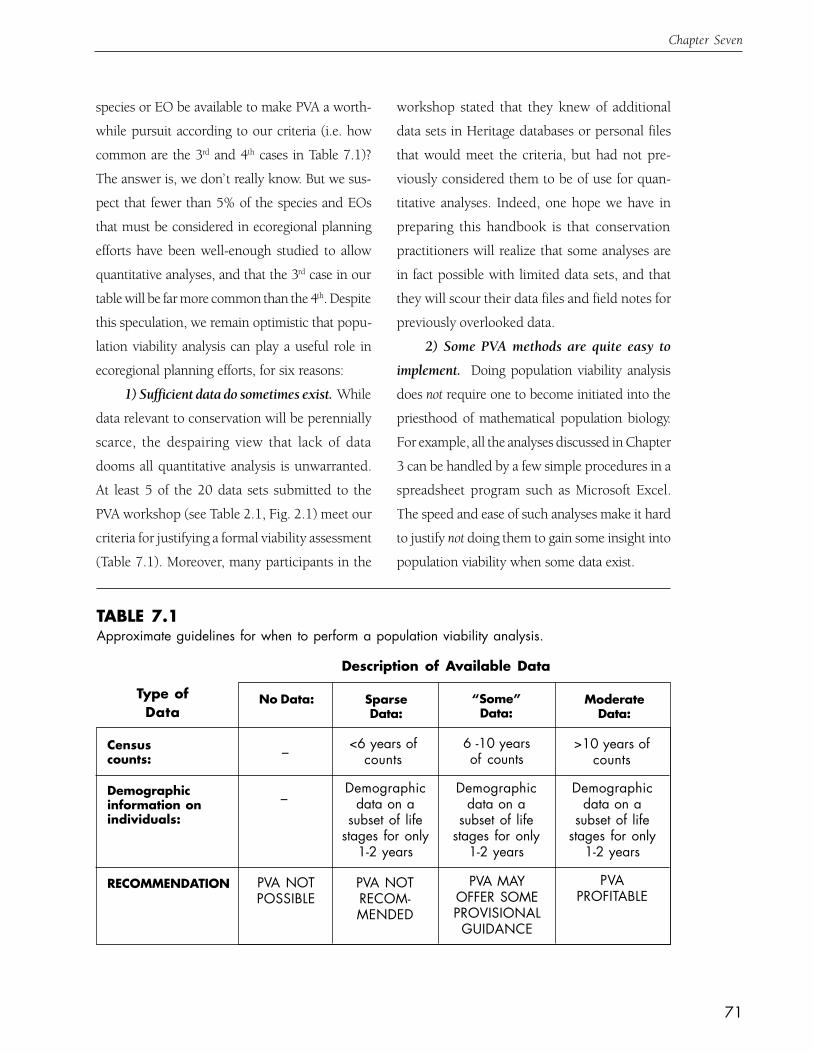
71

Chapter Seven

TABLE 7.1Approximate guidelines for when to perform a population viability analysis.

Type ofData

Description of Available Data

Censuscounts:

Demographicinformation onindividuals:

RECOMMENDATION

_

_

No Data: SparseData:

“Some”Data:

PVA NOTPOSSIBLE

ModerateData:

<6 years ofcounts

Demographicdata on a

subset of lifestages for only

1-2 years



1-2 years



1-2 years

6 -10 yearsof counts

>10 years ofcounts

PVA NOTRECOM-MENDED

PVA MAYOFFER SOMEPROVISIONALGUIDANCE

PVAPROFITABLE

species or EO be available to make PVA a worth-

while pursuit according to our criteria (i.e. how

common are the 3rd and 4th cases in Table 7.1)?

The answer is, we don’t really know. But we sus-

pect that fewer than 5% of the species and EOs

that must be considered in ecoregional planning

efforts have been well-enough studied to allow

quantitative analyses, and that the 3rd case in our

table will be far more common than the 4th. Despite

this speculation, we remain optimistic that popu-

lation viability analysis can play a useful role in

ecoregional planning efforts, for six reasons:

1) Sufficient data do sometimes exist. While

data relevant to conservation will be perennially

scarce, the despairing view that lack of data

dooms all quantitative analysis is unwarranted.

At least 5 of the 20 data sets submitted to the

PVA workshop (see Table 2.1, Fig. 2.1) meet our

criteria for justifying a formal viability assessment

(Table 7.1). Moreover, many participants in the

workshop stated that they knew of additional

data sets in Heritage databases or personal files

that would meet the criteria, but had not pre-

viously considered them to be of use for quan-

titative analyses. Indeed, one hope we have in

preparing this handbook is that conservation

practitioners will realize that some analyses are

in fact possible with limited data sets, and that

they will scour their data files and field notes for

previously overlooked data.

2) Some PVA methods are quite easy to

implement. Doing population viability analysis

does not require one to become initiated into the

priesthood of mathematical population biology.

For example, all the analyses discussed in Chapter

3 can be handled by a few simple procedures in a

spreadsheet program such as Microsoft Excel.

The speed and ease of such analyses make it hard

to justify not doing them to gain some insight into

population viability when some data exist.

72


3) PVAs can be updated. Additional data are

constantly being accumulated, in part as a result

of basic monitoring for rare species. Thus not only

is the number of species that can be subjected to

quantitative analysis likely to increase, but the

quality of previously-performed viability assess-

ments is likely to improve as additional information

is incorporated. As we have repeatedly emphasized,

a strength of quantitative measures of viability not

possessed by more intuitive measures is that we

can easily evaluate how the measures are affected

by changes in our assumptions (for example, if

separate EOs are linked by migration, then viability

assessments made by assuming they are isolated

will overestimate the risk of collective extinction;

see Chapter 5). Thus modest amounts of additional

data (such as the discovery that there is some

migration among EOs, even if we lack estimates of

its magnitude) quickly tell us at least the direction

in which to modify a previously calculated viability

measure. Of course, more detailed information

(e.g. estimates of migration rates, or additional

census counts) would allow us to actually update

the quantitative measures directly.

4) PVA informs the design of monitoring

schemes. Not only do monitoring data improve

the quality of PVAs, but as we have emphasized

in Chapter 6, PVAs can suggest ways to improve

the usefulness and efficiency of monitoring. For

example, projection matrices can tell us which

life stages contribute the most to population

growth; targeting those stages to the exclusion of

less-important ones may be the most efficient

sampling strategy.

5) Viability assessment and management are

connected. The quantitative methods we use to

conduct population viability assessment can do

double duty by helping us to make management

decisions. Projection matrices are the most useful

in this regard, because they can tell us not only

whether the population is on the decline, but

which life stages and which demographic rates

should be the foci for management efforts.

6) PVAs have “strength in numbers”. Quan-

titative analyses of well-studied species or EOs

can inform us about related species or similar

locations about which we have little or no data.

The idea is that by building up a “library” of

viability analyses, we may eventually be able to

place rough bounds on population parameters

(e.g. µ and σ2, see Chapter 3) for groups of species

that share similar life histories, or inhabit similar

environments. We could then ask: “if we know

only the current size of a population of interest,

but we assume its parameters to be similar to

those of ecologically similar species, what is its

relative risk of extinction?” With such comparative

approaches, viability assessments for relatively

well-studied populations may aid us in making

decisions about other, less-studied populations.

With enough estimates of µ and σ2 in our data-

base, we may one day be able to bring more quan-

titative rigor to the process of assigning EO ranks

(A, B, C, and D) for populations about which we

know only the life history of the organism, the

environmental conditions, and the current popu-

lation size.

While we are sanguine about PVA’s potential,

our concern is genuine that users of PVA must not

be blind to the important caveats we have tried to

raise throughout this handbook. To drive this point

home, we review the most important ones below.

73

Chapter Seven

Important Caveats for Users of PVA

1) Viability assessments made with limited amounts

of data will have wide confidence limits (i.e., low

precision)

Although in this handbook we have main-

ly discussed how to calculate direct viability

measures (such as the probability of extinction

over 100 years or the mean time to extinction), it

is critical to remember that these are only estimates,

and that associated with each estimate is a

confidence interval that portrays the most likely

range of values in which the “true” value lies, given

the level of uncertainty in the available data. In

general, the smaller the number of data points

that went into the estimate, the wider the con-

fidence interval will be. To have a true sense of

what the data do (and do not) say about extinction

risk, we should calculate and examine confidence

intervals for our viability measures. While they lie

outside of the scope of this handbook, some

methods to calculate these confidence limits have

been developed for count-based analyses (see

Dennis et al. 1991) and for projection matrix

models (see Chapter 7 in Caswell 1989).

2) Observation errors in the data used to construct

a PVA will influence its predictions.

Errors in counting the number of individuals

in a population, or in measuring demographic rates,

will tend to inflate our estimates of year-to-year

variability, and variability has a major effect on

population persistence (see Chapter 3). In some

cases, we may be able to partition the total varia-

bility in the data into observation error and true

environmental variability (for example, if at each

census the population was sampled several times

over a short period of time; see Chapter 6). But in

most cases, the best we may be able to do is to be

aware of the influence of observation error on our

viability estimates, and to design future monitoring

schemes in such a way that the magnitude of

observation error can be estimated.

3) Rare events (either good years or catastrophes),

although usually omitted from viability analyses,

will affect a population’s extinction risk.

Most quantitative measures of viability ignore

rare events, because there is simply no way to

estimate their frequency or magnitude with limited

data. When presenting viability estimates, we will

almost always need to include the qualifier that

we have not accounted for the potential impact

of floods, fires, extreme storms, unusually favor-

able growing seasons, and other rare events.

4) Real density dependence, if ignored, will cause

resulting viability assessments to be in error.

Many viability assessments assume that the

average population growth rate (e.g. λ in equa-

tion 3.1) is not influenced by population density

(this is as true of the matrix models reviewed in

Chapter 4 as it is of the simple count-based

models in Chapter 3). At some level, this must

be false; no population can grow forever without

straining its resource base and thereby reducing

its own growth rate. At the opposite end of the

density spectrum, low-density populations may

experience higher growth rates because compe-

tition for resources is weak, or lower growth rates

if finding mates becomes difficult. The most

common justifications for omitting density

74


dependence are lack of sufficient data to fit a

density-dependent model and the greater

difficulty of deriving analytical expressions for

extinction measures in models with density

dependence. These and other justifications are

summarized by Groom and Pascual (1998).

Recent theoretical work (e.g. Middleton et al.

1995) is helping to address the second problem.

But when lack of data prevents us from evaluating

density depen-dent models, we should at least

be explicit about this potential source of error.

5) Migration and environmental correlation among

a set of populations will cause the extinction risk

to differ from that of a suite of isolated, independent

populations.

If our data do not allow us to estimate rates

of migration among populations, or the degree

to which population fluctuations are correlated

among populations due to shared environmental

factors, we may be forced to ignore these compli-

cations (see Chapter 5), but we should not ignore

how this omission might influence the predicted

likelihood of collective extinction.

6) Genetics may exert strong effects on population

viability.

As we noted in Chapter 2, while much of

the literature on population viability has empha-

sized genetic problems and concerns, data sets

for rare species almost never include genetic

information. In most cases ignoring genetic pro-

cesses will yield optimistic estimates of viability,

since if inbreeding and inbreeding depression are

significant they will act synergistically with envi-

ronmental variation in driving small populations

extinct (Gilpin and Soule 1986, Mills and

Smouse 1994). However, the past tendency to

dismiss some small populations as inherently

inviable because of predicted genetic conse-

quences is not justified (Lesica and Allendorf

1992, Lande and Barrowclough 1987). In the

absence of genetic information, being aware of

the optimistic effect on viability estimates of ignor-

ing genetic effects may be the best we can do.

The Last Word

Population viability analysis is attractive because

it forces us to define what we mean by phrases

such as “the long-term survival of all viable native

species” (see TNC’s mission statement, Conservation

by Design), and because it provides a way to assess

the likelihood of “long-term survival” using current

population data. But PVA does not provide answers

to all of the questions that will need to be addressed

in designing ecoregional plans. We will often lack

sufficient data to avoid the simplifying assumptions

discussed in the caveats above, and for many

species, population-level data will be completely

absent. Nonetheless, PVA will help us to gain in-

sight into the extinction risks faced by populations

for which we do have data, and those analyses

will help us to assess the viability of less well-

studied populations and species. Ongoing work

in theoretical population biology is constantly lead-

ing to new tools for population viability analysis.

By using the tools of population viability analysis

when data are available, conservation practitioners

might create a “demand” for new methods and tech-

niques that would spur theoretical population bio-

logist to improve existing approaches.

75

REFERENCES

Alvarez-Buylla, E., and M. Slatkin. 1991. Finding confidence limits on population growth rates.Trends in Ecology and Evolution 6: 221-224.

Beier, P. 1993. Determining minimum habitat areas and habitat corridors for cougars. ConservationBiology 7: 94-108.

Beissinger, S. 1995. Modeling extinction in a periodic environment: Everglades water levels andsnail kite population viability. Ecological Applications 5: 618-631.

Berger, J. 1990. Persistence of different-sized populations: an empirical assessment of rapidextinctions in bighorn sheep. Conservation Biology 4:91-98.

Bolger, D.T., A. Alberts, and M.E. Soule. 1991. Occurrence patterns of bird species in habitatfragments: sampling, extinction, and nested species subsets. American Naturalist 137:155-166.

Caswell, H. 1989. Matrix Population Models: construction, analysis and interpretation. Sinauer,Sunderland, MA.

Church, R.L., D.M. Stoms, and F.W. Davis. 1996. Reserve selection as a maximal covering locationproblem. Biological Conservation 76(2): 105-112.

Crouse, D., L. Crowder, and H. Caswell. 1987. A stage-based population model for loggerhead seaturtles and implications for conservation. Ecology 68:1412-1423.

Crowder, L., D. Crouse, S. Heppell, and T. Martin. 1994. Predicting the impact of turtle excluderdevices on loggerhead sea turtle populations. Ecological Applications 4:437-445.

Davis, M.B. and T.R. Simons. 1997. Nest success of American Oystercatcher on Cape LookoutNational Seashore. Report to the National Park Service. NC Cooperative Research Unit,NC State University, Raleigh, NC.

Dennis, B. and M.L. Taper. 1994. Density dependence in time series observations of naturalpopulations: estimation and testing. Ecological Monographs 64: 205-224.

Dennis, B., P.L. Munholland, and J. Michael Scott. 1991. Estimation of growth and extinctionparameters for endangered species. Ecological Monographs 61:115-143.

Doak, D. F. 1995. Source-sink models and the problem of habitat degradation: general models andapplications to the Yellowstone grizzly bear. Conservation Biology 9:1370-1379.

Doak, D. F. and L. S. Mills. 1994. A useful role for theory in conservation. Ecology 75:615-626.

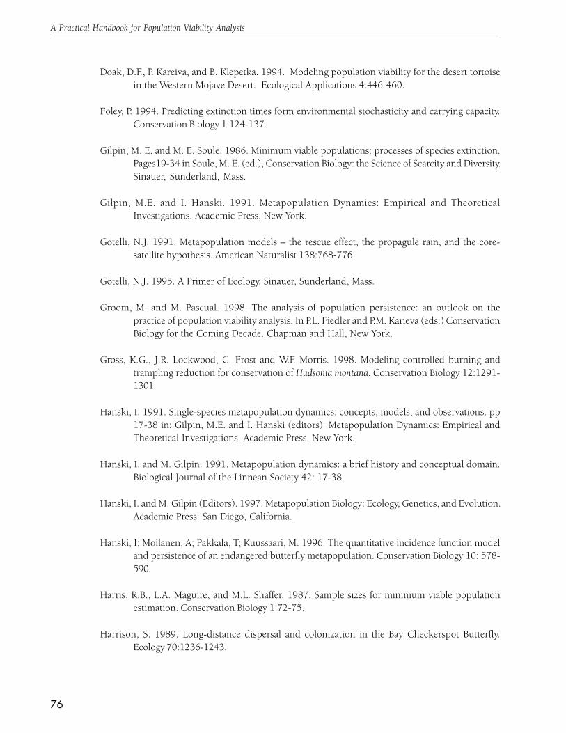
76


Doak, D.F., P. Kareiva, and B. Klepetka. 1994. Modeling population viability for the desert tortoisein the Western Mojave Desert. Ecological Applications 4:446-460.

Foley, P. 1994. Predicting extinction times form environmental stochasticity and carrying capacity.Conservation Biology 1:124-137.

Gilpin, M. E. and M. E. Soule. 1986. Minimum viable populations: processes of species extinction.Pages19-34 in Soule, M. E. (ed.), Conservation Biology: the Science of Scarcity and Diversity.Sinauer, Sunderland, Mass.

Gilpin, M.E. and I. Hanski. 1991. Metapopulation Dynamics: Empirical and TheoreticalInvestigations. Academic Press, New York.

Gotelli, N.J. 1991. Metapopulation models – the rescue effect, the propagule rain, and the core-satellite hypothesis. American Naturalist 138:768-776.

Gotelli, N.J. 1995. A Primer of Ecology. Sinauer, Sunderland, Mass.

Groom, M. and M. Pascual. 1998. The analysis of population persistence: an outlook on thepractice of population viability analysis. In P.L. Fiedler and P.M. Karieva (eds.) ConservationBiology for the Coming Decade. Chapman and Hall, New York.

Gross, K.G., J.R. Lockwood, C. Frost and W.F. Morris. 1998. Modeling controlled burning andtrampling reduction for conservation of Hudsonia montana. Conservation Biology 12:1291-1301.

Hanski, I. 1991. Single-species metapopulation dynamics: concepts, models, and observations. pp17-38 in: Gilpin, M.E. and I. Hanski (editors). Metapopulation Dynamics: Empirical andTheoretical Investigations. Academic Press, New York.

Hanski, I. and M. Gilpin. 1991. Metapopulation dynamics: a brief history and conceptual domain.Biological Journal of the Linnean Society 42: 17-38.

Hanski, I. and M. Gilpin (Editors). 1997. Metapopulation Biology: Ecology, Genetics, and Evolution.Academic Press: San Diego, California.

Hanski, I; Moilanen, A; Pakkala, T; Kuussaari, M. 1996. The quantitative incidence function modeland persistence of an endangered butterfly metapopulation. Conservation Biology 10: 578-590.

Harris, R.B., L.A. Maguire, and M.L. Shaffer. 1987. Sample sizes for minimum viable populationestimation. Conservation Biology 1:72-75.

Harrison, S. 1989. Long-distance dispersal and colonization in the Bay Checkerspot Butterfly.Ecology 70:1236-1243.

77

References

Harrison, S. and J.F. Quinn. 1989. Correlated environments and the persistence of metapopulations.Oikos 56:293-298.

Heppell, S. S. 1998. Application of life-history theory and population model analysis to turtleconservation. Copeia 1998:367-375.

Heyde, C.C., and J.E. Cohen. 1985. Confidence intervals for demographic projections based onproducts of random matrices. Theoretical Population Biology 27:120-53.

Horvitz, C. C., and D. W. Schemske. 1995. Spatiotemporal variation in demographic transitions ofa tropical understory projection matrix analysis. Ecological Monograph 65:155-192.

Krebs, C.J. 1989. Ecological Methodology. Harper & Row, New York.

Kruckeberg, A. R. 1984. California Serpentines: Flora, Vegetation, Geology, Soils, and ManagementProblems. Univ. California Press, Berkeley.

Lamberson, R.H., K. McKelvey, B.R. Noon, and C. Voss. 1992. A dynamic analysis of northernspotted owl viability in a fragmented forest landscape. Conservation Biology 6:505-512.

Lamberson, R. H., B. R. Noon, and K. S. McKelvey. 1994. Reserve design for territorial species – theeffects of patch size and spacing on the viability of the Northern spotted owl. ConservationBiology 8:185-195.

Lande, R. 1988. Demographic models of the Northern Spotted Owl (Strix occidentalis caurina).Oecologia 75:601-607.

Lande, R. 1993. Risks of population extinction from demographic and environmental stochasticityand random catastrophes. Am. Nat. 142:911-927.

Lande, R. and G. F. Barrowclough. 1987. Effective population size, genetic variation, and their usein population management. Pages 87-124 in Soule, M. E. (ed.), Viable Populations forConservation. Cambridge Univ. Press, Cambridge.

Lesica, P. and F. W. Allendorf. 1992. Are small populations of plants worth preserving? ConservationBiology 6:135-139.

Levins, R. 1969. Some demographic and genetic consequences of environmental heterogeneity forbiological control. Bulletin of the Entomological Society of America 15:237-240.

Lindenmayer, D.B., M.A. Burgman, H.R. Akcakaya, R.C. Lacy, and H. Possingham. 1995. A reviewof the generic computer programs ALEX, RAMAS/space and VORTEX for modeling theviability of wildlife metapopulations. Ecological Modeling 82:161-174.

Lindenmeyer, D. B. and H. P. Possingham. 1994. The Risk of Extinction: Ranking managementoptions for Leadbeater’s Possum using population viability analysis. Australian NationalUniversity.

78


Liu, J. G., J. B. Dunning, and H. R. Pulliam. 1995. Potential effects of a forest management plant onBachman’s sparrows (Aimophila aestivalis) – linking a spatially explicit model with GIS.Conservation Biology 9:62-75.

Ludwig, D. 1996. The distribution of population survival times. Am. Nat. 147:506-526.

Mangel, M. and C. Tier. 1993. A simple, direct method for finding persistence times of populationand applications to conservation problems. Proc. Natl. Acad. Sci. USA 90:1083-1086.

Maschinski, J., R. Frye, and S. Rutman. 1997. Demography and population viability of an endangeredplant species before and after protection from trampling. Conservation Biology 11:990-999.

Mattson, D. J., B. M. Blanchard, and R. R. Knight. 1992. Yellowstone grizzly bear mortality, humanhabituation, and whitebark pine seed crops. J. Wildlife Management 56:432-442.

McCullough, D.R. 1996. Metapopulations and Wildlife Conservation. Island Press, Washington,D.C.

Menges, E. 1990. Population Viability Analysis for an endangered plant. Conservation Biology4:52-62.

Middleton, D.A.J., A.R. Veitch, and R.M. Nisbet. 1995. The effect of an upper limit to populationsize on persistence time. Theoretical Population Biology 48: 277-305.

Middleton, D.A.J., and R.M. Nisbet. 1997. Population persistence time: estimates, models andmechanisms. Ecological Applications 7:107-117.

Mills, L.S. and P.E. Smouse. 1994. Demographic consequences of inbreeding in remnant populations.American Naturalist 144:412-431.

Nantel, P., D. Gagnon, and A. Nault. 1996. Population viability analysis of American Ginseng andWild Leek harvested in stochastic environments. Conservation Biology 10:608-621.

Nisbet, R. M. and W. S. C. Gurney. 1982. Modeling Fluctuating Populations. John Wiley, New York.

Panzer, R. and M. W. Schwartz. 1998. Effectiveness of a vegetation-based approach to insectconservation. Conservation Biology 12:693-702.

Pollard, E., K.H. Lakhani, and P. Rothery. 1987. The detection of density-dependence from a seriesof annual censuses. Ecology 68:2146-2155.

Pressey, R.L., H.P. Possingham, and J.R. Day. 1997. Effectiveness of alternative heuristic algorithmsfor identifying indicative minimum requirements for conservation reserves. BiologicalConservation 80:207-219.

79

References

Pulliam, H.R. 1988. Sources, sinks, and population regulation. American Naturalist 132:652-661.

Pulliam, H. R., J. B. Dunning, and J. G. Liu. 1992. Population dynamics in complex landscapes –a case study. Ecological Applications 2:165-177.

Ratsirarson J, J. A. Silander and A. F. Richard. 1996. Conservation and management of a threatenedMadagascar palm species, Neodysis decaryi Jumelle. Conservation Biology 10:40-52.

Ruckelshaus, M, C. Hartway, P. Kareiva. 1997. Assessing the data requirements of spatially explicitdispersal models. Conservation Biology 11:1298-1306.

Schulz, T.T. and A.T. Carpenter (manuscript). Quantifying survival, growth and reproduction ofAletes humilis at Phantom Canyon and Cap Rock Preserves, Colorado. To be submitted toNatural Areas Journal.

Schumaker, N. H. 1998. A User’s Guide to the PATCH Model. USA Environmental ProtectionAgency, Corvallis Oregon.

Shenk, T.M., G.C. White, and K.P. Burnham. 1998. Sampling-variance effects on detecting densitydependence from temporal trends in natural populations. Ecological Monographs 68:445-463.

Southwood, T.R.E. 1978. Ecological Methods. Chapman Hall, New York.

Stacey, P.B. and M. Taper. 1992. Environmental variation and the persistence of small populations.Ecological Applications 2:18-29.

The Nature Conservancy. 1997. Conservation by Design: A Framework for Mission Success.

Tuljapurkar, S. and H. Caswell. 1997. Structured Population Models in Marine, Terrestrial, andFreshwater Systems. Chapman Hall, New York.

Turchin, P. 1998. Quantitative Analysis of Movement: Measuring and Modeling PopulationRedistribution in Animals and Plants. Sinauer, Sunderland, MA.

United States Fish and Wildlife Service. 1993. Grizzly Bear Recovery Plan (and Summary). USDA,Bethesda, Maryland.

Van Horne, B. 1983. Density as a misleading indicator of habitat quality. J. Wildlife Management47:893-901.

Vandermeer, J. 1979. Choosing category size in a stage projection matrix. Oecologia 32:199-225.

Wootton, J. T., and D. A. Bell. 1992. A metapopulation model for the Peregrine Falcon in California:viability and management strategies. Ecological Applications 2:307-321.

A Practical Handbook for Population Viability Analysis · A Practical Handbook for Population...

Documents

Transcript of A Practical Handbook for Population Viability Analysis · A Practical Handbook for Population...