A Practical Guide to Deterministic Particle Methods

Alina Chertock∗

Abstract

The past several decades have seen significant development in the design and numerical analysisof particle methods for approximating solutions of PDEs. In these methods, a numerical solution issought as a linear combination of Dirac delta-functions located at certain points. The locations andcoefficients (weights) of the delta-functions are first chosen to accurately approximate the initial dataand then are evolved in time according to the system of ODEs obtained from a weak formulation ofthe considered problem. The main advantage of the particle methods is their low numerical diffusionthat allows them to capture a variety of nonlinear waves with a high resolution. Even though themost “natural” application of the particle methods is linear transport equations, over the years,the range of these methods has been extended for approximating solutions of convection-diffusionand dispersive equations and general nonlinear problems.

In this paper, we provide a mathematical introduction to deterministic particle methods andreview different aspects of their practical implementation such as recovering an approximate solutionfrom its particle distribution and an investigation of various particle redistribution algorithms.

1 Introduction

In recent years, particle methods have become a useful tool for approximating solutions of PDEs andbeen successfully used to treat a broad class of problems arising in astrophysics, plasma physics, solidstate physics, medical physics, and fluid dynamics; see, e.g., [29,31,58,69–71,73,82,83] and referencestherein. In these methods, the solution is sought as a linear combination of Dirac distributionswhose positions and coefficients represent locations and weights of the particles, respectively. Thesolution is then found by following the time evolution of the locations and the weights of the particlesaccording to a system of ODEs, obtained by considering a weak formulation of the problem. Inorder to recover point values of the the computed solution at some time t > 0, the particle solutionneeds to be regularized, and hence the performance of the particle method depends on the qualityof the regularization procedures, allowing the recovery of the approximate solution from its particledistribution. A commonly used regularization of a particle solution performed by taking a convolutionwith a so-called cut-off function, which plays the role of a smooth approximation to the δ-function andafter a proper scaling takes into account the tightness of the particle discretization. When a particlemethod is applied to problems with nonsmooth data, the reconstruction procedure becomes the mostchallenging part of the overall algorithm — it works perfectly fine for smooth functions, but may breakdown when applied to nonsmooth (discontinuous) solutions.

Mesh-free particle methods have many advantages compared to Eulerian (finite-difference, finite-volume, finite-element etc.) methods. The amount of numerical viscosity introduced by most nonoscil-latory Eulerian discretizations of the convective terms may seriously degrade the accuracy of a com-putational method especially if a coarse grid is forced to be used. Lagrangian-type methods, on theother hand, can ameliorate most of the problems posed by the presence of numerical viscosity sinceparticles provide a non-dissipative approximation of the convection. Furthermore, in some scientific

∗Department of Mathematics, North Carolina State University, Raleigh, NC 27695, USA chertock@math.ncsu.edu

1

2 A. Chertock

applications, such as kinetic theory, for instance, FD schemes cannot be applied to a realistic case,because of the dimensionality of the problem [33], while in particle schemes, the particles are concen-trated in the relevant region of the phase space, optimizing the memory storage of the computer. Asmesh-free, particle methods are also very flexible, and, therefore beneficial, when problems with verycomplicated geometries and/or moving boundaries are considered.

Particle methods have been used for a long time to give a numerical solution of purely convectiveproblems, such as the incompressible Euler equation in fluid mechanics [70, 82, 83] or the Vlasovequation in plasma physics [61]. Over the years, the range of particle methods has been extendedto treat other type of equations including convection-diffusion, dispersive and others and we referthe reader to several books and survey monographs, where a large variety of particle-type methodsare being reviewed, see,e.g., [40, 84, 95] and references therein. Particle method approximations ofhyperbolic PDEs with oscillatory solutions were studied in [54]. A detailed description of particlemethods with an emphasis on vortex methods and smooth particle hydrodynamics (SPH) and theirapplications can also be found in [40,94].

It is generally possible to divide the particle methods for convection-diffusion equations into twoclasses: stochastic and deterministic ones. The most widely used treatment of diffusion terms, therandom vortex method, was developed in [30]. There, diffusion was introduced by adding a Wienerprocess to the motion of each vortex. Numerous works followed that pioneering paper and propertiesof the random vortex method have been extensively studied in the literature (for a comprehensivelist we refer the reader to [101] and [40]). Several deterministic methods have been explored fortreating the diffusion terms in particle schemes. Among them is the so-called weighted particle method[42, 43, 49, 90, 91]), in which the convective part of the equation is modeled by the convection of theparticles, while the diffusion part of the equation is taken into account by changing the particleweights. Another example is the diffusion-velocity method, which is based on defining the convectivefield associated with the heat operator which then allowed the particles to convect in a standardway ( [50, 78, 79, 86]), and others ( [34, 52, 53, 59, 104–106]). In this case, the PDE is rewritten asif it was an advection equation with a speed that depends on the solution and its derivatives. Thesolution is then obtained by implementing the particle method with the only difference being that thepoint values of the computed solution should be recovered from the particle distribution at every timestep during the time integration (unlike linear advection problems, in which the solution is recoveredonly at the final time). The diffusion-velocity particle method has been also applied to linear andnonlinear dispersive equations as well as used for direct simulations of solitary waves interactions, see,e.g., [12, 16,24–28,47,48,92].

One must be aware, however, that the self-adaptivity of the particle positions to the local flowmap comes at the expense of the regularity of the particle distribution: inter-particle distances maychange in time, and just as particles may cluster in the immediate region of the discontinuity they mayspread too far from each other near nonsmooth fronts. This may lead not only to a poor resolution ofthe computed solution, but also to an extremely low efficiency of the methods. The latter is relatedto the fact that the time step for the ODE solver used to evolve the particle system in time depends,in general, on the distance between the particles. The success of various particle i methods reliesthus not only upon accurate reconstruction procedures used to recover point values of the numericalsolution from its particle distribution, but also upon accurate and efficient redistribution algorithms,which will ensure that different regions in the computational domain are adequately resolved. A largevariety of remeshing techniques were proposed in the literature over the last decades including bothglobal interpolation-type methods, see, e.g, [7–10, 14, 37, 37, 38, 40, 40, 41, 44, 44, 45, 65, 74, 76, 80, 88,93, 96–98, 100, 100, 102, 108, 110, 111] and local particle merger algorithms, see, e.g., [23, 81, 109]. it isalso well-known that particle methods encounter difficulties in the accurate treatment of boundaryconditions, while their adaptivity is often associated with severe particle distortion that may introducespurious scales. Recent research efforts that attempt to address these issues are outlined in [75].

A Practical Guide to Particle Methods 3

There are many applications, for which a hybridization of the Eulerian and Lagrangian approachesmay be beneficial or even crucial for achieving high resolution of the computed solution since particlemethods have their own applicability limitations if the considered problems involve additional termsbesides linear convection (e.g. collision terms, diffusion, or dispersion, and/or nonlinear terms). Hybridmethods involve combination of mesh-based schemes and particle methods in an effort to utilize thespecific advantages of each part of the hybrid method in the right place, see, e.g., [15, 17–20, 22, 35,36, 46, 70, 97]. It should also be noted, that since in many problems where some sharp interfaces areneeded to be captured, the use of particle methods may be critical for obtaining a high resolution ofthe computed solution due to the low dissipativeness nature of these methods, see also [55,56,72,77].

The purpose of this manuscript is to provide a mathematical review of deterministic particle meth-ods for advection equations as well as to discuss various aspects related to the practical implementationof these methods. The paper is organized as follows: We start, in Section 2, with a description of de-terministic particle methods in the context of linear transport equations and provide a review of majoranalytical results. We then discuss, in Section 3, various remeshing techniques that ensure consistent,efficient, and accurate simulations by particle methods. We conclude, in Section 4, with particleapproximations for derivative operators, which are presented in the context of convection-diffusionequations.

2 Description of the Particle Method

In this section, we describe the derivation of the particle method using the example of linear transportequation, here written in the divergence form:

ut +∇x · (au) + a0u = S, x ∈ Rd, t > 0, (2.1)

and considered subject to initial data

u0(x) := u(x, 0), (2.2)

where, u is an unknown function of a time variable t and d-spatial variables x = (x1, . . . , xd)T , the

velocity vector a = (a1(x, t), . . . , ad(x, t))T , the coefficient a0(x, t), and the source/sink term S(x, t)

are given functions.

As it was mentioned above, the main idea of the particle methods is to seek a solution of a PDEas a linear combination of Dirac distributions,

uN (x, t) =

N∑i=1

wi(t) δ(x− xi(t)),

for some set (xi(t), wi(t)) of points xi(t) ∈ Rd and coefficients wi(t) ∈ R that are chosen at time t = 0to accurately approximate the initial data and then evolved in time according to the system of ODEsobtained from a weak formulation of the underlying PDE. Such solutions are called particle solutionsand the δ-functions in the above formula are called particles. The coefficients wi(t) are called particleweights, since they represent the amount of the physical quantity u, carried by the ith particle, whichis located at xi(t) at time t, and N is the total number of particles. It should be emphasized that theintroduced particles are mathematical objects rather than (physical) particles of a certain material. Animportant step in implementation of particle methods is the recovery of point values of the computedsolution from its particle distribution. In what follow, we describe each one of the aforementionedsteps, i.e., initialization, evolution and reconstruction.

4 A. Chertock

2.1 Particle Approximation of the Initial Data

The first step in the derivation of the particle method consists of approximating the initial data (2.2)by a linear combination of Dirac distributions:

uN0 (x) =N∑i=1

wi(0) δ(x− xi(0)), (2.3)

where wi(0) are given coefficients and xi(0) are the initial locations of the δ-functions. This can bedone, for instance, in the sense of measures. Namely, for any test function φ ∈ C0

0 (Ω), the innerproduct (u0(·), φ(·)) should be approximated by

∫Ω

u0(x)φ(x) dx ≈ (uN0 (·), φ(·)) =

N∑i=1

wi(0)φ(x). (2.4)

Based on (2.4), we observe that that determining the initial weights, wi(0), is exactly equivalent tosolving a standard numerical quadrature problem. One way of solving this problem is to first divide

the computational domain Ω into a set of N nonoverlapping subdomains Ωi:N⋃i=1

Ωi = Ω, Ωi⋂

Ωl =

∅, ∀i 6= l. Then the location of the ith particle, xi(0), is set at the center of mass of Ωi and the entiremass of u0 in Ωi is ”placed” into the ith particle so that its initial weight is

wi(0) :=

∫Ωi

u0(x) dx. (2.5)

For instance, one can take

wi(0) = |Ωi|u0(xi(0)),

which will correspond to the midpoint rule for (2.5). In general, one can build a sequence of basisfunctions that will aid in solving the numerical quadrature problem given by (2.4), see, e.g., [26, 27].One may also prove (see, e.g., [26, 40,103]) that uN0 converges weakly to u0 as N →∞, i.e., if

maxi|Ωi| → 0 as N →∞, (2.6)

then for all φ ∈ C00 (Ω)

limN→∞

∫Ω

(uN0 (x)− u0(x))φ(x) dx = 0.

2.2 Time Evolution of Particles

As it was mentioned above, particle methods are obtained by considering a weak formulation of theunderlying problem and therefore we start by defining a weak solution of (2.1), (2.2). Following [103],we denote by M(Ω) the space of measures defined on Ω ⊂ Rd, that is, the space dual to the spaceC0

0 (Ω) of continuous functions Ω → R with compact support. A weak solution is then defined asfollows.

A Practical Guide to Particle Methods 5

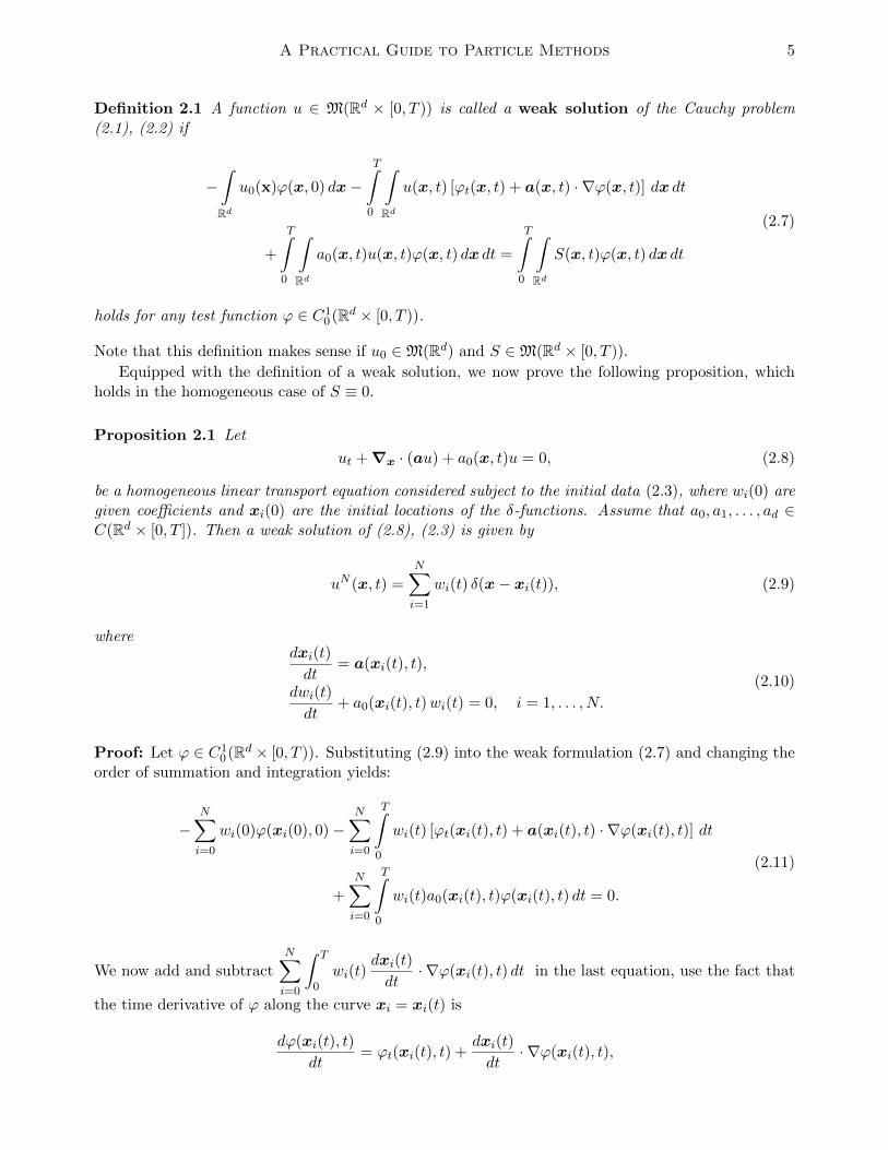
Definition 2.1 A function u ∈ M(Rd × [0, T )) is called a weak solution of the Cauchy problem(2.1), (2.2) if

−∫Rd

u0(x)ϕ(x, 0) dx−T∫

0

∫Rd

u(x, t) [ϕt(x, t) + a(x, t) · ∇ϕ(x, t)] dx dt

+

T∫0

∫Rd

a0(x, t)u(x, t)ϕ(x, t) dx dt =

T∫0

∫Rd

S(x, t)ϕ(x, t) dx dt

(2.7)

holds for any test function ϕ ∈ C10 (Rd × [0, T )).

Note that this definition makes sense if u0 ∈M(Rd) and S ∈M(Rd × [0, T )).

Equipped with the definition of a weak solution, we now prove the following proposition, whichholds in the homogeneous case of S ≡ 0.

Proposition 2.1 Let

ut + ∇x · (au) + a0(x, t)u = 0, (2.8)

be a homogeneous linear transport equation considered subject to the initial data (2.3), where wi(0) aregiven coefficients and xi(0) are the initial locations of the δ-functions. Assume that a0, a1, . . . , ad ∈C(Rd × [0, T ]). Then a weak solution of (2.8), (2.3) is given by

uN (x, t) =N∑i=1

wi(t) δ(x− xi(t)), (2.9)

wheredxi(t)

dt= a(xi(t), t),

dwi(t)

dt+ a0(xi(t), t)wi(t) = 0, i = 1, . . . , N.

(2.10)

Proof: Let ϕ ∈ C10 (Rd × [0, T )). Substituting (2.9) into the weak formulation (2.7) and changing the

order of summation and integration yields:

−N∑i=0

wi(0)ϕ(xi(0), 0)−N∑i=0

T∫0

wi(t) [ϕt(xi(t), t) + a(xi(t), t) · ∇ϕ(xi(t), t)] dt

+

N∑i=0

T∫0

wi(t)a0(xi(t), t)ϕ(xi(t), t) dt = 0.

(2.11)

We now add and subtractN∑i=0

∫ T

0wi(t)

dxi(t)

dt· ∇ϕ(xi(t), t) dt in the last equation, use the fact that

the time derivative of ϕ along the curve xi = xi(t) is

dϕ(xi(t), t)

dt= ϕt(xi(t), t) +

dxi(t)

dt· ∇ϕ(xi(t), t),

6 A. Chertock

and rewrite equation (2.11) as follows:

−N∑i=0

wi(0)ϕ(xi(0), 0)−N∑i=0

T∫0

wi(t)dϕ(xi(t), t)

dtdt

+

N∑i=0

T∫0

wi(t)

[dxi(t)

dt− a(xi(t), t)

]· ∇ϕ(xi(t), t) dt+

N∑i=0

T∫0

wi(t)a0(xi(t), t)ϕ(xi(t), t) dt = 0.

(2.12)Integrating by parts the second term in the first row in (2.12) and rearranging other terms, we finallyobtain:

N∑i=0

T∫0

wi(t)

[dxi(t)

dt− u(xi(t), t)

]· ∇ϕ(xi(t), t) dt

+N∑i=0

T∫0

[dwi(t)

dt+ wi(t)a0(xi(t), t)

]ϕ(xi(t), t) dt = 0.

(2.13)

Since the functions xi(t) and wi(t) satisfy the system (2.10), the last equation holds for any ϕ implyingthat uN defined by (2.9), (2.10) is a weak solution of (2.8), (2.3). This completes the proof.

In the general case of S 6= 0, a particle solution of (2.1), (2.2) is obtained by solving the initial-valueproblem (2.1), (2.3), whose solution uN (x, t) is still given by (2.9), but the locations and weights ofthe particles satisfy a different system of ODEs (compare with the system (2.10)):

dxi(t)

dt= a(xi(t), t),

dwi(t)

dt+ a0(xi(t), t)wi(t) = βi(t),

(2.14)

where βi reflects the contribution of the source term S (see, e.g., [32,103]). To evaluate βi, we considera particle approximation of S, given by

S(x, t) ≈ SN (x, t) :=N∑i=1

βi(t) δ(x− xi(t)),

where

βi(t) =

∫Ωi(t)

S(x, t) dx ≈ S(xi(t), t) |Ωi(t)|. (2.15)

Here, Ωi(t) is the subdomain of Ω that includes the ith particle and should satisfy the following twoproperties for all t (not only at t = 0):

Ω =N⋃i=1

Ωi(t), Ωi(t)⋂

Ωl(t) = ∅, ∀i 6= l, wi(t) ≈∫

Ωi(t)

u(x, t) dx.

These requirements are hard to guarantee, but noticing that in order to use (2.15) only the size ofΩi(t) is needed, one may apply the Liouville theorem (see, e.g., [3, 31]) to obtain the following ODE

d

dt|Ωi(t)| = ∇x · a(xi(t), t) |Ωi(t)|, (2.16)

which has to be solved together with the system (2.14) to complete the construction of the particlemethod.

A Practical Guide to Particle Methods 7

Remark 2.1 We note that in the case when the velocity vector field u is divergence-free, that is,when ∇x · a ≡ 0, the size of the ith subdomain does not change, that is, |Ωi(t)| ≡ |Ωi| ∀t. Otherwise,|Ωi(t)| changes in time and the coefficients (weights) βi in (2.15) would depend on t even when thesource S = S(x) only.

Remark 2.2 It should be observed that in practice, except in very special cases, the functions xi(t)and wi(t) have to be determined numerically. In fact, the ODE system (2.10) can be solved by meansof a classical numerical method using one’s favorite ODE solver.

The above discussion leads to the following algorithm for obtaining a particle solution of (2.1), (2.2):

• Divide the computational domain Ω into a set of N nonoverlapping subdomains Ωi:

N⋃i=1

Ωi = Ω, Ωi⋂

Ωl = ∅, ∀i 6= l.

• Replace the the initial datum u0 in (2.2) by its particle approximation uN0 , (2.3),

for some set (xi(0), wi(0)) of points xi(0) in the computational domain Ω and weights

wi(0) computed according to (2.5).

• If S ≡ 0 in the right-hand side of equation (2.1), consider the system (2.8), (2.3)

and obtain its particle solution (2.9) by numerically integrating the system of ODEs

(2.10).

• If S 6= 0, replace S(x, 0) with its particle approximation to compute the coefficients

βi(0) according to (2.15) with t = 0. Consider the system (2.1), (2.3) and obtain

its particle solution (2.9) by numerically solving the system of ODEs (2.14)-(2.16).

Finally, the basic convergence result for particle methods is stated in the following theorem.

Theorem 2.1 Consider equation (2.8) with the coefficients ai ∈ L∞(0, T ;W 1,∞(Ω)), i = 1, . . . , d anda0 ∈ L∞(Ω × (0, T )). Let the initial condition u0 ∈ C0(Ω) and its particle approximation is given by(2.3). Then, for all ϕ ∈ C0

0 (Ω)

limN→∞

∫Ω

(u(x, t)− uN (x, t))ϕ(x) dx = 0 uniformly in t ∈ [0, T ].

Theorem 2.1 guarantees that for sufficiently regular coefficients a, a0 and initial datum w0, theparticle solution will converge to the exact one in the sense of measures. However, the above result isof little use when one is interested in obtaining point values of the computed solution. In this respect,it is more useful to associate the particle solution uN (·, t) with a continuous function uNε (·, t), whichapproximates the solution u(·, t) in a more classical sense. In a next section we provide an example ofhow such an approximation can be constructed.

2.3 Particle Function Approximations

The regularization of particle solution is usually performed by taking a convolution product with amollification kernel (or, so-called, cut-off function), ζε(x), that after a proper scaling takes into accountthe initial tightness of the particle discretization, namely,

u(x, t) ≈ uε(x, t) := (u(·, t) ∗ ζε(·))(x) =

∫u(y, t)ζε(x− y) dy, (2.17)

8 A. Chertock

where ζε ∈ C0(Rd)⋂L1(Rd) satisfies the following properties

ζε(x) :=1

εdζ(xε

),

∫Rd

ζ(x) dx = 1, (2.18)

and ε denotes a characteristic length of the kernel, see, e.g., [103]. The particle approximation of theregularized solution is then defined as

u(x, t) ≈ uNε (x, t) := (uN (·, t) ∗ ζε(·))(x) =N∑i=1

wi(t)ζε(x− xi(t)). (2.19)

It is clear from the above discussion that the approximation of the computed solution by formula(2.19) is one of the key ingredients of the particle method and hence, the performance of the methoddepends on the quality of this smoothing procedure. The error introduced by the quadrature (2.19)of the mollified approximation uNε for the function u can be divided into two parts:

u− uNε = (u− u ∗ ζε) + (u− uN ) ∗ ζε. (2.20)

The first term in equation (2.20) denotes the mollification error that can be controlled by appropriatelyselecting the kernel properties. The second term denotes the quadrature error due to the approximationof the integral in (2.17) on the particle location. The accuracy of the particle method will thus berelated to the moments of ζ that are being conserved, and we say that the kernel is of order k when:

∫Rd

ζ(x) dx = 1,

∫Rd

xαζ(x) dx = 0, for all multiindexes α such that 1 ≤ |α| ≤ k − 1,

∫Rd

|x|k|ζ(x)| dx <∞.

(2.21)

Example 2.1 (Gaussian and Generalized Gaussian) A (generalized) Gaussian can be consid-ered as an example of a cut-off function and is obtained by taking the inverse Fourier transform of the

function e−|ξ|2l

, where l ∈ N and ξ ∈ Rd:

ζl(x) = Cl

∫Rd

eix·ξ e−|ξ|2ldξ. (2.22)

Taking an appropriate normalizing coefficient Cl, one can ensure that the C∞-functions ζl, whichrapidly decay at ∞, satisfy the conditions (2.21) with k = 2l. Thus, these mollifiers are of order l. Inparticular, when l = 1 we obtain the first-order Gaussian

ζ1(x) =1

πd/2e−|x|

2.

When l = 2, (2.22) reduces to the second-order super-Gaussian, which in the one-dimensional (1-D)case reads

ζ2(x) =1√π

(3

2− x2

)e−x

2.

A Practical Guide to Particle Methods 9

Example 2.2 (Compactly Supported Mollifiers) The simplest example of a compactly supported1-D cut-off function is the quadratic B-spline:

ζ(x) =

3

4− x2, |x| ≤ 1

2,

1

2

(3

2− |x|

)2

,1

2≤ |x| ≤ 3

2,

0, otherwise.

For this cut-off function k = 2, and thus it is only first-order accurate. An advantage of compactlysupported cut-off functions is that it is easy to implement the summation in (2.19) in a very efficientway, which is one of the crucial points in practical implementation of particle methods. Higher ordercompactly supported kernels can be obtained by ensuring that more moments are conserved and canbe found in, e.g., [40, 88,93].

There is an extensive discussion in the literature on the selection of a cut-off function and itsrelation to the overall accuracy of particle methods, [5–7,30,40,66,68,101]. See also [1,32,49,50,67,75,91,93,94,96,98,103]. Obviously, the accuracy of the particle method will depend both on the choice ofcut-off function (2.18) and on its width ε as it is given by the following theorem [103] (note that similarerror estimates can also be obtained for compactly supported cut-off functions, see, e.g., [57, 103]).

Theorem 2.2 Let (2.21) are satisfied for some integer k ≥ 1. Assume that both ζ and the coefficientsin (2.1) are sufficiently smooth, more precisely: ζ ∈ Wm,∞(Rd)

⋂Wm,1(Rd) for some integer m > d

and a1, . . . , ad, a0 + ∇ · a ∈ L∞(0, T ;W l,∞(Rd)), where l = max(k,m). Then, if the initial datumis also smooth (u0 ∈ W l,p(Rd)), then there exists a positive constant C = C(T ), such that for anyt ∈ [0, T ],

‖u− uNε ‖Lp(Rd) ≤ Cεk ‖u0‖k,p,Rd +

(h

ε

)m‖u0‖m,p,Rd

, (2.23)

where h > 0 is the size of nonoverlapping d-dimensional cubes covering Rd.

Accuracy. The two terms in the error estimate (2.23) may be balanced by choosing an appropriatesize of ε. Intuitively, it is clear that if the smoothing parameter ε is too small in comparison to theminimal distance between particles, the approximate solution defined by (2.19) will vanish away fromthe ε-neighborhood of the particles and is thus irrelevant. On the other hand, large values of ε willgenerate unacceptable smoothing errors. Theoretically ε is chosen so that the smoothing error and thediscretization error are of the same order and it is common to take ε ∼

√h, see, e.g., [20, 21, 67, 103].

It should be noted, however, that it is not clear what the optimal proportionality constant is. Thatstrongly depends on both the smoothness of the flow and the cut-off function and its value at the origin.It has been also observed in various numerical experiments that the overall accuracy of the particlemethod can deteriorate over long time integrations, see, e.g., the discussion in [7,65,67,75,96,98] andin references therein.

Smooth vs. discontinuous solutions. The procedure for point values recovery described aboveprovides an optimal order of accuracy when the captured solution is sufficiently smooth. However,when a and/or u in (2.1) are discontinuous, approximation (2.19) may be inaccurate and even unac-ceptable, as it has been demonstrated in [18,20,22]. In order to overcome this difficulty, the convolutionprocedure (2.19) can be, for instance, modified by taking kernels of locally varying width, whose sizewas selected in a point-wise manner depending on the distance between the particles, [8, 20, 39, 74].Another approach for recovering point values of the computed solution from its particle distribution is

10 A. Chertock

based on interpreting the particle data as integrals of the approximated solution over some nonover-lapping domains around the particles, see, e.g., [18, 22]. Then, the averaged values of the numericalsolution can be obtained dividing the weights wi(t) by the volumes of the corresponding domains.We also refer the reader to [41], where total variation diminishing (TVD) reconstruction formulae fordiscontinuous solutions were proposed for particle methods in the context of nonlinear conservationlaws.

Efficiency. Besides the accuracy of particle methods, the computational speed is also important.The most time-consuming aspect in particle simulations is accurately evaluating the long-range inter-actions of particles that appear in the summation formula (2.19). The direct method of computingvalues of the cut-off function requires O(N2) flops, where N is the total number of particles. Thereis a number of fast summation algorithms known to reduce the computational cost of the particlemethod to O(N logN). Example of such methods include particle-mesh techniques that account forparticles in close proximity in terms of grid spacing, see, e.g. [73] and references therein. There arealso mesh-free fast summation techniques that are based on the concept of multipole end Taylor ex-pansions, see, e.g., [2, 4, 13, 63, 85]. These methods employ clustering of particles and use expansionsof the potentials around the cluster centers with a limited number of terms to calculate their far-fieldinfluence onto other particles. These techniques rely on tree data structures to achieve computationalefficiency. The tree allows a spatial grouping of the particles, and the interactions of well-separatedparticles is computed using their center of mass or multipole and Taylor expansions.

3 Remeshing for Particle Distortion

As evidenced by the foregoing discussion, the time evolution of particle positions is dictated by thegradients of the flow field and, as the result, inter-particle distances constantly change. This self-adaptation of particles to the local flow map comes at the expense of the regularity of their distri-bution since particles may either spread away from each other or cluster in the regions of the largevelocity gradients or near discontinuities even if the velocity function a is a smooth function of itsarguments. This becomes a critical issue in preserving the accuracy of particle methods and theirefficient implementation.

While the lack of particles in certain areas may result in deterioration of the accuracy of the methodand poor resolution of the computed solution (appearance of artificial vacuum areas), local particleaccumulations may lead to an extremely low efficiency of the method making it almost impractical.The latter is related to the fact that the time step of numerical ODE solvers for (2.10) (or (2.14))depends on the distance between the particles as the stability condition imposes that no characteristiccurves or their trajectories should intersect in finite time. The latter leads to a time-step constraintof the type

∆t ≤ C‖∇a‖−1∞ , (3.1)

where C depends on the specific numerical solver used. As the result, the success of various particlemethods relies not only upon accurate reconstruction procedures used to recover numerical solutionfrom its particle distribution but also upon accurate and efficient particle redistribution algorithms,which will ensure that different regions in the computational domain are adequately resolved.

The redistribution of particles is in general performed through interpolation formulae and consistsof (occasional) re-initialization (remeshing) of particle locations onto a new regularized set of particlesand recalculating the particle weights on these new locations. The resulting problem of extractinginformation on a regular grid from a set of scattered points has a long history and we refer the reader toan extensive list of redistribution algorithms, which are based on various techniques ranging from globalrezoning using fixed, one-sided and variable size kernels, see, e.g., [7, 40, 44, 65, 74, 93, 96, 98, 100, 108]

A Practical Guide to Particle Methods 11

and particle-mesh methods, see, e.g., [9,10,14,37,37,38,40,41,44,45,76,80,88,97,100,102,110,111] tomultilevel adaptive particle methods, see, e.g., [8, 75] and references therein.

3.1 Particle Weights Redistribution

For completeness of the presentation, we provide here several examples that illustrate basic, yet com-monly used, global and local remeshing ideas. To this end, we denote by xiNi=1 and xjJj=1 re-spectively the old (distorted) and the new (regular) set of particles and we denote by wi and wj thecorresponding particle weights at the old and new locations at certain time t. For the sake of sim-plicity, we also assume that the new particles, xj(t), lie at the centers of the nonoverlapping cells,

CjJi=1,J⋃j=1

Cj = Ω, Cj⋂Cl = ∅, ∀j 6= l, of size h that cover the computational domain Ω.

Convolution. One of the simplest and natural ways of computing new particle weights wj is to re-initialize particle approximation (2.19) at the new nodes by just replacing x by xj(t) in the formula,that is,

uNε (xj(t), t) =N∑i=1

wi(t)ζε(xj(t)− xi(t)), j = 1, . . . , J, (3.2)

see, e.g., [7, 20,24,25,40,74,93,96]. Using the relation

wj(t) =

∫Cj

u(x, t) dx, (3.3)

the new weights can be recomputed by, say, the midpoint rule as wj(t∗) = huNε (xj(t), t), ∀j = 1, . . . , J ,

and then the particle method is restarted.

Interpolation. Another widespread redistribution procedure is based on a classical interpolationrule:

wj(t) =

N∑i=1

wi(t) Φ

(|xj(t)− xi(t)|

h

), j = 1, . . . , J, (3.4)

where Φ is an interpolation kernel whose properties determine the type and the quality of the redis-tribution procedure and is typically designed to conserve a certain number of moments of the particledistribution, see, e.g., [20,21,23,40,73,93,99,107]. This technique (unlike the previously described con-volution approach) is in particularly appealing in applications, where, conservation of total amount ofu may be crucial for designing a good numerical method. In the context of redistribution of particles,the conservation requirement can be stated as

J∑j=1

wj(t) =N∑i=1

wi(t). (3.5)

There are many choices for Φ(r) that ensure (3.5) and we consult here [99] to bring two particularexamples: a first-order:

Φ(r) =

1

8

(5− 2r −

√−7 + 12r − 4r2

), if |r| < 1,

1

8

(3− 2r −

√1 + 4r − 4r2

), if 1 < |r| < 2,

0, otherwise

12 A. Chertock

and a second-order kernel:

Φ(r) =

φ(r), |r| < 1,

1

6r3 − 7

8r2 +

7

12r +

21

16− 3

2φ(r − 1), 1 < |r| < 2,

− 1

12r3 +

3

4r2 − 23

12r +

9

8+

1

2φ(r − 2), 2 < |r| < 3,

0, otherwise,

with

φ(r) =1

12r3 − 11

56r2 − 11

42r +

61

112+

1

336

√3(−112r6 + 336r5 + 500r4 − 1560r3 − 748r2 + 1584r + 243).

Remark 3.1 Both the convolution and redistribution techniques described above are global (all par-ticle locations and weights are changed) and are not limited to uniform auxiliary grids and allow toobtain point values of the computed particle approximation at any prescribed set of points. Thesemethods would, in general, work perfectly fine in smooth regions, yet may smear out discontinuitiesthat may appear in the solution or develop oscillations near nonsmooth fronts.

Remark 3.2 The time scale on which remeshing is done is mostly empirical. It is clearly correlatedto the strain rate (velocity gradient) of the flow and constrained by (3.1). A simple rule that provedto be efficient in various calculations is to remesh every few time steps or even at the end of everytime step. It should be observed, however, that if a redistribution procedure is applied too often,the overall resolution of the computed solution may deteriorate. Therefore, one has to come up withan (ad-hoc) strategy on when to redistribute particles, for instance, one may apply the redistributionprocedure either when the smallest/largest distance between the particles becomes smaller/larger thana prescribed critical value. Additional strategies can be found in, e.g., [7, 20, 21, 23–25, 40, 41, 88, 96]and references therein.

3.2 Particle Merger — a Local Redistribution Technique

The major drawback of the aforementioned global redistribution techniques is numerical diffusionbrought to the particle method every time the locations of the particles are changed and the weightsare recalculated. This may be unavoidable in the case of spreading particles, but when the particlescluster, another redistribution technique — merger of clustering particles — may be used to improvethe efficiency of the particle method, see, e.g., [23, 81, 109]. Particle merger techniques seem also towork perfectly well for the models with point mass concentrations and strong singularity formations(δ-functions along the surface as well as at separate points) as it was demonstrated in [23], wherea sticky particle method was introduced in the context of the Euler equations of pressureless gasdynamics, [11, 112].

The simplest particle merger algorithm can be described as follows, [23]. When at a certain time t,the distance |xi(t)−xj(t)| is smaller then a prescribed (ad-hoc) parameter for some i and j, then theith and jth particles are merged into a new partcle located, say, at the center of mass of the replacedparticles, i.e.,

x =wi(t)xi(t) + wj(t)xj(t)

wi(t) + wj(t)

and carrying the weightw = wi(t) + wj(t).

A Practical Guide to Particle Methods 13

The cell occupied by the new particle is then set to be the union of Ωi(t) and Ωj(t):

|Ω| = |Ωi(t)|+ |Ωj(t)|.

It should be noted that this particle merging procedure also serves as an excellent discontinuitiesdetector — as long as the number of particles stays equal to the initial number of particles, thesolution can be assumed continuous, but after the merger occurs, we assume that a discontinuity hasbeen already formed. Moreover, by keeping a record of the location of particle, one may track thediscontinuity location as well. Obviously, in large time simulations, the overall accuracy of the methodmay decrease due to particle mergers, since the overall number of particles decreases in time. In sucha case, one would need to periodically add new particles into the smooth parts of the solution.

4 Applications to Convection-Diffusion Equations

Even though the most natural application of the particle methods is pure transport equations, overthe years, the range of these methods has been extended. Many practical problems involve additionalterms, besides convection (e.g. collision terms or diffusion), and hence, a demand for particle meth-ods, which are capable to treat diffusion, dispersion and general nonlinear terms was created. As aconsequence, the original particle method has been modified in a number of different ways and severalapproaches have been suggested for approximating derivatives as the latter became a key aspect inthe development of particle methods.

The most widely used treatment of diffusion terms, the random vortex method, was introducedin [30]. In this method, the diffusion is treated by adding a Wiener process to the motion of eachparticle. This way the diffusion only affects the position of particles, xi(t), while the particle weights,wi(t), remain constant in time. Numerous works followed this pioneering paper (see, e.g., [1, 5–7, 62,64, 66, 68, 83, 87, 96]). Properties of the random vortex method have been also extensively studied inthe literature. For a comprehensive list we refer to [40,101].

Deterministic particle approximations of the derivative operators can be constructed, for instance,through the integral approximations. This can be easily achieved by taking the derivatives in equation(2.19) as convolution and derivative operators commute in unbounded or periodic domains. These ap-proximations can be cast in a conservative formulation and have been implemented in various versionsof particle methods (like, e.g., SPH [94, 95]). An alternative formulation involves the development ofintegral operators that are equivalent to differential operators. We review here both approaches in thecontext of convection-diffusion while leaving the discussion of other particle approximations out of thescope of this paper.

4.1 Particle Methods for Convection-Diffusion Equations

We consider the following convection-diffusion equation:

ut + ∇x · (au) = ν∆u, ν > 0, (4.1)

which is studied subject to the initial condition (2.2) and explore two deterministic methods for treatingthe diffusion terms in particle schemes.

4.1.1 Weighted Particle Method

In the so-called weighted particle method proposed in [49] (see also [42, 91]), the convective part ofthe equation is modeled by the convection of particles, while the diffusion part is taken into account

14 A. Chertock

by changing the weights of the particles. This deterministic particle method is then based on thefollowing integro-differential approximation of the convection-diffusion equation (4.1):

uσt + ∇x · (auσ) = ν∆σuσ, (4.2)

where

∆σuσ :=1

σ2

∫Rd

ησ(x− y) (u(y)− u(x)) dy, (4.3)

and the function

ησ(x) =1

σdη(xσ

),

where η ∈ L1(Rd) is an even function, that is, η(−x) = η(x) for all x ∈ Rd.The main idea of the weighted particle method is to apply the particle method to equation (4.2)

(instead of the original equation (4.1)) and to treat the modified viscosity ν∆σuσ as a source term.Substituting the particle expansion (2.9) into a weak formulation of (4.3), leads to the following systemof ODEs for the particle locations and their weights:

dxi(t)

dt= a(xi(t), t),

dwi(t)

dt= βi(t), i = 1, . . . , N,

where

βi(t) =ν

σ2

N∑j=1

ησ(xi(t)− xj(t)) wj(t)|Ωi(t)| − wi(t)|Ωj(t)| ,

and |Ωj(t)| is still given by (2.16).Convergence properties of the weighted particle method have been investigated in [49], where the

convergence of the solution of problem (4.2) towards the solution of (4.1) has been proven and thestability and convergence results for the weighted particle method in L∞ have been established.

Remark 4.1 The weighted particle method has been applied to first-order systems in [51,89,90] andto the systems of gas dynamics in [60].

Remark 4.2 Starting from this formulation, a general deterministic integral representation for deriva-tives of arbitrary order was presented in [53].

Remark 4.3 A different technique in which particle methods were used for approximating solutions ofthe heat equation and related models (such as the Fokker-Planck equation, a Boltzmann-like equation– the Kac equation and Navier-Stokes equations), was introduced in [104, 105]. In these works, thediffusion of the particles was described as a deterministic process in terms of a mean motion with aspeed equal to the osmotic velocity associated with the diffusion process. In a following work, [106], themethod was shown to be successful for approximating solutions to the 2-D Navier-Stokes equation inan unbounded domain. In this setup, the particles were convected according to the velocity field whiletheir weights evolved according to the diffusion term in the vorticity formulation of the Navier-Stokesequations.

We also refer to [59] where a different way to discretize viscous terms of the Navier-Stokes equationswas suggested. The idea was to approximate the Laplacian of the vorticity by the explicit differentia-tion of the cut-off function. Another approach, see for example [34, 52, 53], is based on discretizationof an integro-differential equation in which an integral operator approximates the diffusion operator.

A Practical Guide to Particle Methods 15

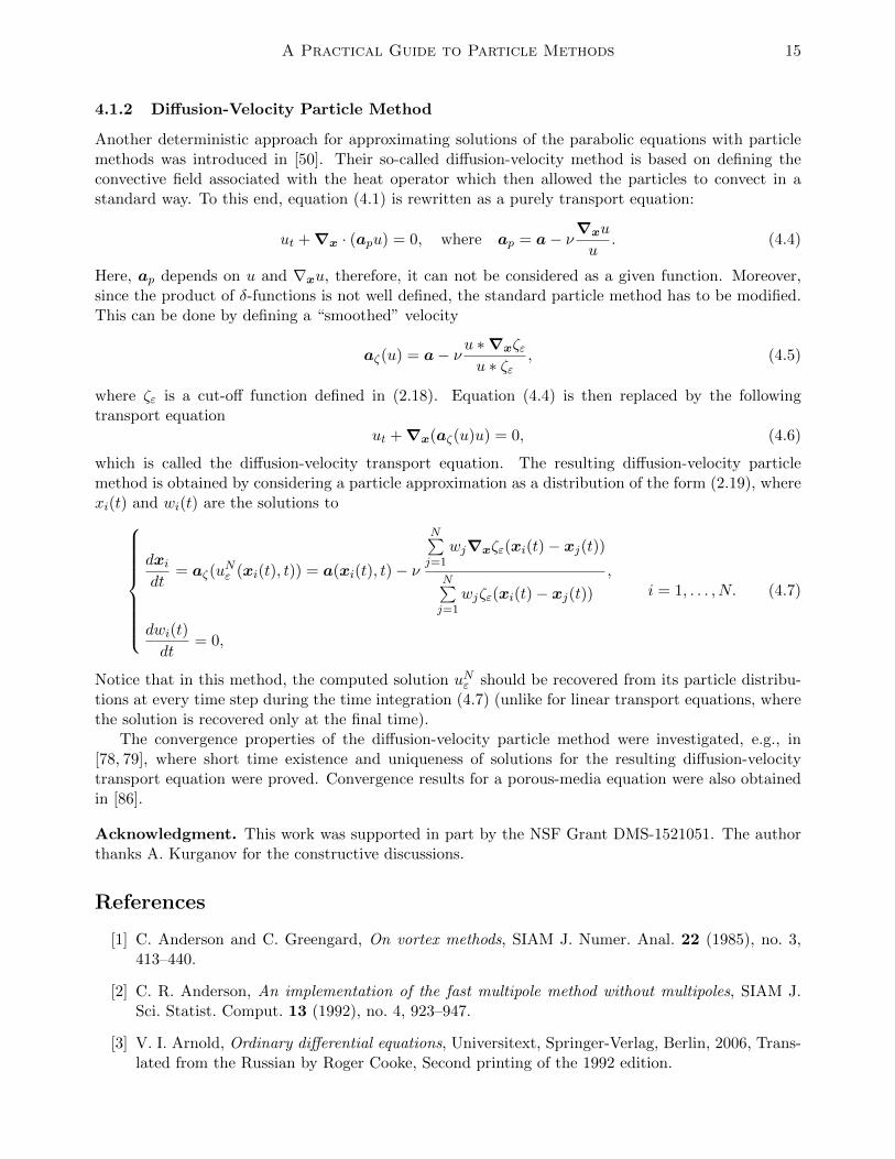
4.1.2 Diffusion-Velocity Particle Method

Another deterministic approach for approximating solutions of the parabolic equations with particlemethods was introduced in [50]. Their so-called diffusion-velocity method is based on defining theconvective field associated with the heat operator which then allowed the particles to convect in astandard way. To this end, equation (4.1) is rewritten as a purely transport equation:

ut + ∇x · (apu) = 0, where ap = a− ν∇xu

u. (4.4)

Here, ap depends on u and ∇xu, therefore, it can not be considered as a given function. Moreover,since the product of δ-functions is not well defined, the standard particle method has to be modified.This can be done by defining a “smoothed” velocity

aζ(u) = a− ν u ∗∇xζεu ∗ ζε

, (4.5)

where ζε is a cut-off function defined in (2.18). Equation (4.4) is then replaced by the followingtransport equation

ut + ∇x(aζ(u)u) = 0, (4.6)

which is called the diffusion-velocity transport equation. The resulting diffusion-velocity particlemethod is obtained by considering a particle approximation as a distribution of the form (2.19), wherexi(t) and wi(t) are the solutions to

dxidt

= aζ(uNε (xi(t), t)) = a(xi(t), t)− ν

N∑j=1

wj∇xζε(xi(t)− xj(t))

N∑j=1

wjζε(xi(t)− xj(t))

,

dwi(t)

dt= 0,

i = 1, . . . , N. (4.7)

Notice that in this method, the computed solution uNε should be recovered from its particle distribu-tions at every time step during the time integration (4.7) (unlike for linear transport equations, wherethe solution is recovered only at the final time).

The convergence properties of the diffusion-velocity particle method were investigated, e.g., in[78, 79], where short time existence and uniqueness of solutions for the resulting diffusion-velocitytransport equation were proved. Convergence results for a porous-media equation were also obtainedin [86].

Acknowledgment. This work was supported in part by the NSF Grant DMS-1521051. The authorthanks A. Kurganov for the constructive discussions.

References

[1] C. Anderson and C. Greengard, On vortex methods, SIAM J. Numer. Anal. 22 (1985), no. 3,413–440.

[2] C. R. Anderson, An implementation of the fast multipole method without multipoles, SIAM J.Sci. Statist. Comput. 13 (1992), no. 4, 923–947.

[3] V. I. Arnold, Ordinary differential equations, Universitext, Springer-Verlag, Berlin, 2006, Trans-lated from the Russian by Roger Cooke, Second printing of the 1992 edition.

16 A. Chertock

[4] J. Barnes and P. Hut, A hierarchical O(N log N) force-calculation algorithm, nature 324 (1986),no. 6096, 446–449.

[5] J. T. Beale and A. Majda, Vortex methods. I. Convergence in three dimensions, Math. Comp.39 (1982), no. 159, 1–27.

[6] , Vortex methods. II. Higher order accuracy in two and three dimensions, Math. Comp.39 (1982), no. 159, 29–52.

[7] , High order accurate vortex methods with explicit velocity kernels, J. Comput. Phys. 58(1985), 188–208.

[8] M. Bergdorf, G.-H. Cottet, and P. Koumoutsakos, Multilevel adaptive particle methods forconvection-diffusion equations, Multiscale Model. Simul. 4 (2005), no. 1, 328–357.

[9] M. Bergdorf and P. Koumoutsakos, A Lagrangian particle-wavelet method, Multiscale Model.Simul. 5 (2006), no. 3, 980–995.

[10] , Multiresolution particle methods, Complex effects in large eddy simulations, Lect. NotesComput. Sci. Eng., vol. 56, Springer, Berlin, 2007, pp. 49–61.

[11] Y. Brenier and E. Grenier, Sticky particles and scalar conservation laws, SIAM J. Numer. Anal.35 (1998), 2317–2328.

[12] R. Camassa, J. Huang, and L. Lee, On a completely integrable numerical scheme for a nonlinearshallow-water wave equation, J. Nonlinear Math. Phys. 12 (2005), no. suppl. 1, 146–162.

[13] J. Carrier, L. Greengard, and V. Rokhlin, A fast adaptive multipole algorithm for particle sim-ulations, SIAM J. Sci. Statist. Comput. 9 (1988), no. 4, 669–686.

[14] P. Chatelain, G.-H. Cottet, and P. Koumoutsakos, Particle mesh hydrodynamics for astrophysicssimulations, Internat. J. Modern Phys. C 18 (2007), no. 4, 610–618.

[15] A. Chertock, C. R. Doering, E. Kashdan, and A. Kurganov, A fast explicit operator splittingmethod for passive scalar advection, J. Sci. Comput. 45 (2010), 200–214.

[16] A. Chertock, P. Du Toit, and J. E. Marsden, Integration of the EPDiff equation by particlemethods, ESAIM Math. Model. Numer. Anal. 46 (2012), no. 3, 515–534.

[17] A. Chertock, E. Kashdan, and A. Kurganov, Propagation of diffusing pollutant by a hybridEulerian-Lagrangian method, Hyperbolic problems: theory, numerics, applications, Springer,Berlin, 2008, pp. 371–379.

[18] A. Chertock and A. Kurganov, On a hybrid finite-volume particle method, M2AN Math. Model.Numer. Anal 38 (2004), 1071–1091.

[19] , Conservative locally moving mesh method for multifluid flows, Finite Volumes for Com-plex Applications IV (F. Benkhaldoun, D. Ouazar, and S. Raghay, eds.), Hermes Science, 2005,pp. 273–284.

[20] , On a practical implementation of particle methods, Appl. Numer. Math. 56 (2006),1418–1431.

[21] , Computing multivalued solutions of pressureless gas dynamics by deterministic particlemethods, Commun. Comput. Phys. 5 (2009), 565–581.

A Practical Guide to Particle Methods 17

[22] A. Chertock, A. Kurganov, and G. Petrova, Finite-volume-particle methods for models of trans-port of pollutant in shallow water, J. Sci. Comput. 27 (2006), 189–199.

[23] A. Chertock, A. Kurganov, and Yu. Rykov, A new sticky particle method for pressureless gasdynamics, SIAM J. Numer. Anal. 45 (2007), 2408–2441.

[24] A. Chertock and D. Levy, Particle methods for dispersive equations, J. Comput. Phys. 171(2001), no. 2, 708–730.

[25] , A particle method for the KdV equation, J. Sci. Comput. 17 (2002), 491–499.

[26] A. Chertock, J.-G. Liu, and T. Pendleton, Convergence analysis of the particle method for theCamassa-Holm equation, Proceedings of the 13th International Conference on “Hyperbolic Prob-lems: Theory, Numerics and Applications” (Ph. G. Ciarlet and Ta-Tsien Li, eds.), ContemporaryApplied Mathematics, 2012, pp. 356–373.

[27] , Convergence of a particle method and global weak solutions of a family of evolutionaryPDEs, SIAM J. Numer. Anal. 50 (2012), no. 1, 1–21.

[28] , Elastic collisions among peakon solutions for the Camassa-Holm equation, Appl. Numer.Math. 93 (2015), 30–46.

[29] J. P. Choquin and S. Huberson, Particle simulation of viscous flow, Comput. & Fluids 17 (1989),no. 2, 397–410.

[30] A. J. Chorin, Numerical study of slightly viscous flow, J. Fluid Mech. 57 (1973), no. 4, 785–796.

[31] A. J. Chorin and J. E. Marsden, A mathematical introduction to fluid mechanics, third ed., Textsin Applied Mathematics, vol. 4, Springer-Verlag, New York, 1993.

[32] A. Cohen and B. Perthame, Optimal approximations of transport equations by particle and pseu-doparticle methods, SIAM J. Math. Anal. 32 (2000), no. 3, 616–636.

[33] M. H. Cohen and A. Robertson, Wave propagation in the early stages of aggregation of cellularslime molds, J. Theor. Biol. 31 (1971), 101–118.

[34] R. Cortez, Convergence of high-order deterministic particle methods for the convection-diffusionequation, Comm. Pure Appl. Math. 50 (1997), no. 12, 1235–1260.

[35] G.-H. Cottet, A particle-grid superposition method for the Navier-Stokes equations, J. Comput.Phys. 89 (1990), no. 2, 301–318.

[36] , A particle model for fluid-structure interaction, C. R. Math. Acad. Sci. Paris 335 (2002),no. 10, 833–838.

[37] G.-H. Cottet, G. Balarac, and M. Coquerelle, Subgrid particle resolution for the turbulent trans-port of a passive scalar, pp. 779–782, Springer Berlin Heidelberg, Berlin, Heidelberg, 2009.

[38] G.-H. Cottet, J.-M. Etancelin, F. Perignon, and C. Picard, High order semi-Lagrangian particlemethods for transport equations: numerical analysis and implementation issues, ESAIM Math.Model. Numer. Anal. 48 (2014), no. 4, 1029–1060.

[39] G.-H. Cottet, P. Koumoutsakos, and M. L. O. Salihi, Vortex methods with spatially varying cores,J. Comput. Phys. 162 (2000), no. 1, 164–185.

18 A. Chertock

[40] G.-H. Cottet and P. D. Koumoutsakos, Vortex methods, Cambridge University Press, Cambridge,2000.

[41] G.-H. Cottet and A. Magni, TVD remeshing formulas for particle methods, C. R. Math. Acad.Sci. Paris 347 (2009), no. 23-24, 1367–1372.

[42] G.-H. Cottet and S. Mas-Gallic, A particle method to solve transport-diffusion equations, part 1:the linear case, Tech. Report 115, Ecole Polytechnique, Palaiseau, France, 1983.

[43] , A particle method to solve the Navier-Stokes system, Numer. Math. 57 (1990), no. 8,805–827.

[44] G.-H. Cottet and P. Poncet, Advances in direct numerical simulations of 3D wall-bounded flowsby vortex-in-cell methods, J. Comput. Phys. 193 (2004), no. 1, 136–158.

[45] G.-H. Cottet and L. Weynans, Particle methods revisited: a class of high order finite-differencemethods, C. R. Math. Acad. Sci. Paris 343 (2006), no. 1, 51–56.

[46] S. Cui, A. Kurganov, and A. Medovikov, Particle methods for PDEs arising in financial modeling,Appl. Numer. Math. (2015), 123–139.

[47] A. Degasperis, D. D. Holm, and A. N. W. Hone, A new integrable equation with peakon solutions,Theoret. Math. Phys. 133 (2002), 1463–1474.

[48] A. Degasperis and M. Procesi, Asymptotic integrability, Symmetry and perturbation theory(Rome, 1998), World Sci. Publ., River Edge, NJ, 1999, pp. 23–37.

[49] P. Degond and S. Mas-Gallic, The weighted particle method for convection-diffusion equations.part 1 and part 2, Math. Comp. 53 (1989), 485–525.

[50] P. Degond and F. J. Mustieles, A deterministic approximation of diffusion equations using par-ticles, SIAM J. Sci. Stat. Comp. 11 (1990), no. 2, 293–310.

[51] P. Degond and B. Niclot, Numerical analysis of the weighted particle method applied to thesemiconductor boltzmann equation, Numer. Math. 55 (1989), no. 5, 599–618.

[52] J. D. Eldredge, T. Colonius, and A. Leonard, A vortex particle method for two-dimensionalcompressible flow, J. Comput. Phys. 179 (2002), no. 2, 371–399.

[53] J. D. Eldridge, A. Leonard, and T. Colonious, A general deterministic treatment of derivativesin particle methods, J. Comput. Phys. 180 (2002), no. 2, 686–709.

[54] B. Engquist and T. Y. Hou, Particle method approximation of oscillatory solutions to hyperbolicdifferential equations, SIAM J. Numer. Anal. 26 (1989), no. 2, 289–319.

[55] D. Enright, R. Fedkiw, J. Ferziger, and I. Mitchell, A hybrid particle level set method for improvedinterface capturing, J. Comput. Phys. 183 (2002), no. 1, 83–116.

[56] D. Enright, F. Losasso, and R. Fedkiw, A fast and accurate semi-Lagrangian particle level setmethod, Comput. & Structures 83 (2005), no. 6-7, 479–490.

[57] L. C. Evans, Partial differential equations, Graduate Studies in Mathematics, vol. 19, AmericanMathematical Society, Providence, RI, 1998.

[58] M. W. Evans and F. H. Harlow, The particle-in-cell method for hydrodynamic calculations, Tech.Report LA-2139, Los Alamos Scientific Laboratory, 1957.

A Practical Guide to Particle Methods 19

[59] D. Fishelov, A new vortex scheme for viscous flows, J. Comput. Phys. 86 (1990), 211–224.

[60] R. J. Gingold and J. J. Monaghan, Shock simulation by the particle method S.P.H., J. Comput.Phys. 37 (1987), 374–389.

[61] R. T. Glassey, The Cauchy problem in kinetic theory, Society for Industrial and Applied Math-ematics (SIAM), Philadelphia, PA, 1996.

[62] J. Goodman, Convergence of the random vortex method, Comm. Pure Appl. Math. 40 (1987),no. 2, 189–220.

[63] L. Greengard and V. Rokhlin, The rapid evaluation of potential fields in three dimensions, Vortexmethods (Los Angeles, CA, 1987), Lecture Notes in Math., vol. 1360, Springer, Berlin, 1988,pp. 121–141.

[64] K. Gustafson and J. Sethian, Vortex methods and vortex motion, SIAM, Philadelphia, 1991.

[65] O. Hald and V. M. del Prete, Convergence of vortex methods for Euler’s equations, Math. Comp.32 (1978), no. 143, 791–809.

[66] O. H. Hald, Convergence of vortex methods for Euler’s equations. II, SIAM J. Numer. Anal. 16(1979), no. 5, 726–755.

[67] , Convergence of vortex methods for Euler’s equations. III, SIAM J. Numer. Anal. 24(1987), no. 3, 538–582.

[68] , Convergence of vortex methods, Vortex methods and vortex motion, SIAM, Philadelphia,PA, 1991, pp. 33–58.

[69] F. H. Harlow, A machine calculation method for hydrodynamic problems, Tech. Report LAMS-1956, Los Alamos Scientific Laboratory, 1956.

[70] , The particle-in-cell computing method for fluid dynamics, Methods in ComputationalPhysics (B. Alder, S. Fernbach, and M. Rotenberg, eds.), vol. 3, Academic Press, New York,1964, pp. 319–343.

[71] F. Hermeline, A deterministic particle method for transport diffusion equations: Application tothe fokker-planck equation, J. Comput. Phys 82 (1989), no. 1, 122–146.

[72] S. E. Hieber and P. Koumoutsakos, A Lagrangian particle level set method, J. Comput. Phys.210 (2005), no. 1, 342–367.

[73] R. W Hockney and J. W Eastwood, Computer simulation using particles, CRC Press, 2010.

[74] T. Y. Hou, Convergence of a variable blob vortex method for the Euler and Navier-Stokes equa-tions, SIAM J. Numer. Anal. 27 (1990), no. 6, 1387–1404.

[75] P. Koumoutsakos, Multiscale flow simulations using particles, Annual review of fluid mechanics.Vol. 37, Annu. Rev. Fluid Mech., vol. 37, Annual Reviews, Palo Alto, CA, 2005, pp. 457–487.

[76] P. Koumoutsakos and A. Leonard, High-resolution simulations of the flow around an impulsivelystarted cylinder using vortex methods, Journal of Fluid Mechanics 296 (1995), 1–38.

[77] R. Krasny, A study of singularity formation in a vortex sheet by the point-vortex approximation,J. Fluid Mech. 167 (1986), 65–93.

20 A. Chertock

[78] G. Lacombe, Analyse d’une equation de vitesse de diffusion, C. R. Acad. Sci. Paris Ser. I Math.329 (1999), no. 5, 383–386.

[79] G. Lacombe and S. Mas-Gallic, Presentation and analysis of a diffusion-velocity method, Flowsand related numerical methods (Toulouse, 1998), ESAIM Proc., vol. 7, Soc. Math. Appl. Indust.,Paris, 1999, pp. 225–233 (electronic).

[80] J.-B. Lagaert, G. Balarac, and G.-H. Cottet, Hybrid spectral-particle method for the turbulenttransport of a passive scalar, J. Comput. Phys. 260 (2014), 127–142.

[81] G. Lapenta, Particle rezoning for multidimensional kinetic particle-in-cell simulations, J. Com-put. Phys. 181 (2002), 317–337.

[82] A. Leonard, Vortex methods for flow simulation, J. Comput. Phys. 37 (1980), no. 3, 289–335.

[83] , Computing three-dimensional incompressible flows with vortex elements, Ann. Rev.Fluid Mech. 17 (1985), 289–335.

[84] S. Li and W. K. Liu, Meshfree particle methods, Springer-Verlag, Berlin, 2004.

[85] K. Lindsay and R. Krasny, A particle method and adaptive treecode for vortex sheet motion inthree-dimensional flow, J. Comput. Phys. 172 (2001), no. 2, 879–907.

[86] P.-L. Lions and S. Mas-Gallic, Une methode particulaire deterministe pour des equations diffu-sives non lineaires, C. R. Acad. Sci. Paris Ser. I Math. 332 (2001), no. 4, 369–376.

[87] D.-G. Long, Convergence of the random vortex method in two dimensions, J. Amer. Math. Soc.1 (1988), no. 4, 779–804.

[88] A. Magni and G.-H. Cottet, Accurate, non-oscillatory, remeshing schemes for particle methods,J. Comput. Phys. 231 (2012), no. 1, 152–172.

[89] S. Mas-Gallic, A deterministic particle method for the linearized boltzmann equation, TransportTheory and Stat. Phys. 16 (1987), 855–887.

[90] S. Mas-Gallic and F. Poupaud, Approximation of the transport equation by a weighted particlemethod, Transport Theory and Stat. Phys. 17 (1988), 311–345.

[91] S. Mas-Gallic and P. A. Raviart, Particle approximation of convection-diffusion equations, In-ternational Report 86013, Universite Pierre et Marie Curie, 1986.

[92] R. McLachlan and S. Marsland, N -particle dynamics of the Euler equations for planar diffeo-morfism, Dyn. Syst. 22 (2007), no. 3, 269–290.

[93] J. J. Monaghan, Extrapolating B-splines for interpolation, J. Comput. Phys. 60 (1985), no. 2,253–262.

[94] , Particle methods for hydrodynamics, Comp. Phys. Rep. 3 (1985), no. 2, 71–124.

[95] , An introduction to sph, Comp. Phys. Commun. 48 (1988), no. 1, 89–96.

[96] H. Nordmark, Rezoning for higher order vortex methods, J. Comput. Phys. 97 (1991), 366–397.

[97] M. L. Ould-Salihi, G.-H. Cottet, and M. El Hamraoui, Blending finite-difference and vortexmethods for incompressible flow computations, SIAM J. Sci. Comput. 22 (2000), no. 5, 1655–1674 (electronic).

A Practical Guide to Particle Methods 21

[98] M. Perlman, On the accuracy of vortex methods, J. Comput. Phys. 59 (1985), no. 2, 200–223.

[99] C. S. Peskin, The immersed boundary method, Acta Numer. 11 (2002), 479–517.

[100] P. Ploumhans, G. S. Winckelmans, J. K. Salmon, A. Leonard, and M. S. Warren, Vortex methodsfor direct numerical simulation of three-dimensional bluff body flows: application to the sphereat Re = 300, 500, and 1000, J. Comput. Phys. 178 (2002), no. 2, 427–463.

[101] E. G. Puckett, Vortex methods - an introduction survey of selected research topics, Incompressiblecomputational fluid dynamics - Trends and advances (M.D. Gunzburger and R.A. Nicolaides,eds.), Cambridge University Press, 1993, pp. 335–407.

[102] J. T. Rasmussen, G.-H. Cottet, and J. H. Walther, A multiresolution remeshed Vortex-In-Cellalgorithm using patches, J. Comput. Phys. 230 (2011), no. 17, 6742–6755.

[103] P.-A. Raviart, An analysis of particle methods, Numerical methods in fluid dynamics (Como,1983), Lecture Notes in Math., vol. 1127, Springer, Berlin, 1985, pp. 243–324.

[104] G. Russo, Deterministic diffusion of particles, Comm. Pure Appl. Math. 43 (1990), 697–733.

[105] , A particle method for collisional kinetic equations. I. Basic theory and one-dimensionalresults, J. Comput. Phys. 87 (1990), 270–300.

[106] , A deterministic vortex method for the Navier-Stokes equations, J. Comput. Phys. 108(1993), 87–95.

[107] I. J. Schoenberg, Cardinal spline interpolation, Society for Industrial and Applied Mathematics,Philadelphia, Pa., 1973, Conference Board of the Mathematical Sciences Regional ConferenceSeries in Applied Mathematics, No. 12.

[108] J. Strain, 2D vortex methods and singular quadrature rules, J. Comput. Phys. 124 (1996), no. 1,131–145.

[109] J. Teunissen and U. Ebert, Controlling the weights of simulation particles: adaptive particlemanagement using k-d trees, J. Comput. Phys. 259 (2014), 318–330.

[110] W. M. van Rees, A. Leonard, D. I. Pullin, and P. Koumoutsakos, A comparison of vortex andpseudo-spectral methods for the simulation of periodic vortical flows at high Reynolds numbers,J. Comput. Phys. 230 (2011), no. 8, 2794–2805.

[111] D. Wee and A. F. Ghoniem, Modified interpolation kernels for treating diffusion and remeshingin vortex methods, J. Comput. Phys. 213 (2006), no. 1, 239–263.

[112] Ya. B. Zeldovich, Gravitational instability: An approximate theory for large density perturbations,Astron. Astrophys. 5 (1970), 84–89.