A Potential Function Approach to the Flow of Play Soccer

Journal of Quantitative Analysis inSports

Volume3, Issue1 2007 Article 3

A Potential Function Approach to the Flow ofPlay in Soccer

David R. Brillinger∗

∗University of California, Berkeley, [email protected]

Copyright c©2007 The Berkeley Electronic Press. All rights reserved.

A Potential Function Approach to the Flow ofPlay in Soccer∗

David R. Brillinger

Abstract

There is a growing literature on the statistical analysis of data from association-football/soccergames, seasons or groups of seasons. In contrast this paper is concerned with a single play, thatis a sequence of successful passes. The play studied contained 25 passes and ended in a goal forArgentina in World Cup 2006. One question addressed is how to describe analytically the spatial-temporal movement of such a particular sequence of passes.

The basic data are points in the plane, successively joined by straight lines. The resulting fig-ure represents the trajectory of the moving soccer ball. The approach of this study is to develop auseful potential function, a concept arising from physics and engineering. In particular the poten-tial function leads to a regression model that may be fit directly by linear least squares.

The resulting potential function may be used for simple description, summary, comparison, sim-ulation, prediction, model appraisal, bootstrapping, and employed for estimating quantities ofinterest. The purpose illustrated here is to simulate play in a game where the ball goes back andforth between two teams each having their own potential function.

KEYWORDS: Argentina, association football, exploratory data analysis, potential function, re-gression model, Serbia-Montenegro, simulation, soccer, vector field, World Cup 2006, 25-passplay.

∗I wish to thank Tatyana Shepova of Online Media Technologies Limited for providing additionaldetail on the play, beyond those in the standard World 3D Cup 2006 Player package. I also wish tothank the Referees and the Editor for various pithy remarks. The work was supported by the NSFGrant DMS-200504162.

1. Introduction The 2006 World Cup included some grand moments. One of the most spectacular was the 25-pass scoring play of Argentina in the Serbia-Montenegro (S-M) game on 16 June. The shot that ended the play was a goal scored by Cambiasso, but some 8 players worked hard to get the ball into position for his shot. The play has been described as: “one of the all time great World Cup goals”, “the play of the tournament”, “a joy forever”, “a glorious goal”, “mesmerizing”, and “a string of pearls”. Not long after the game, sketches of the path of the ball started to appear in newspapers (e.g. Expressen, Sweden) and magazines (e.g. Cambio, Columbia). Purposes of this paper are to develop an analytic description and model for such a play and to explore its uses, e.g. for simulation of plays where the ball changes sides. The play began in the Argentine half of the field with Maxi passing back to Heinze. The sequence of players involved then was: Mascherano, Riquelme, Maxi, Sorin, Maxi, Sorin, Mascherano, Riquelme, Ayala, Maxi, Mascherano, Maxi, Sorin, Maxi, Cambiasso, Riquelme, Mascherano, Sorin, Saviola, Riquelme, Saviola, Cambiasso, Crespo, Cambiasso with Cambiasso scoring. Maxi was involved 6 times, while Requilme, Masherano and Sorin contributed 4 passes each. Videos of the goal may be found at YouTube, see YouTube (2006a, 2006b). Figure 1 below provides the estimated locations of where the passes initiated during the play. (How the estimation was carried out will be described below.) The locations are denoted by small circles. Straight lines join them in order of time. The track is meant to represent the path of the ball being played about the field as seen from above. One notes that the ball generally moved towards the S-M goal with passes going off in many directions and some back passes being made. There are no very short passes, the shortest being 5.6m . There is a growing literature on the statistical modeling of aspects of soccer matches. One highly quoted study was performed by Reep and Benjamin (1968). They investigated data on goal scoring and lengths of passing sequences from 3213 games. They summarize the counts of successful passes by the negative binomial distribution and, for example, conclude that “it takes 10 shots to score 1 goal.” Hughes, M. and Franks, I. (2005) describe the Reep and Benjamin paper as a “landmark”, but in a discussion of the ‘long-ball game’ versus ‘direct play’ complain about various of Reep and Benjamin’s conclusions and their impact.

1

Brillinger: The Flow of Play in Soccer

Published by The Berkeley Electronic Press, 2007

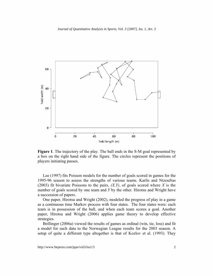
Figure 1. The trajectory of the play. The ball ends in the S-M goal represented by a box on the right hand side of the figure. The circles represent the positions of players initiating passes. Lee (1997) fits Poisson models for the number of goals scored in games for the 1995-96 season to assess the strengths of various teams. Karlis and Ntzoufras (2003) fit bivariate Poissons to the pairs, (X,Y), of goals scored where X is the number of goals scored by one team and Y by the other. Hirotsu and Wright have a succession of papers. One paper, Hirotsu and Wright (2002), modeled the progress of play in a game as a continuous time Markov process with four states. The four states were: each team is in possession of the ball, and when each team scores a goal. Another paper, Hirotsu and Wright (2006) applies game theory to develop effective strategies. Brillinger (2006a) viewed the results of games as ordinal (win, tie, loss) and fit a model for such data to the Norwegian League results for the 2003 season. A setup of quite a different type altogether is that of Kozlov et al. (1993). They

2

Journal of Quantitative Analysis in Sports, Vol. 3 [2007], Iss. 1, Art. 3

http://www.bepress.com/jqas/vol3/iss1/3

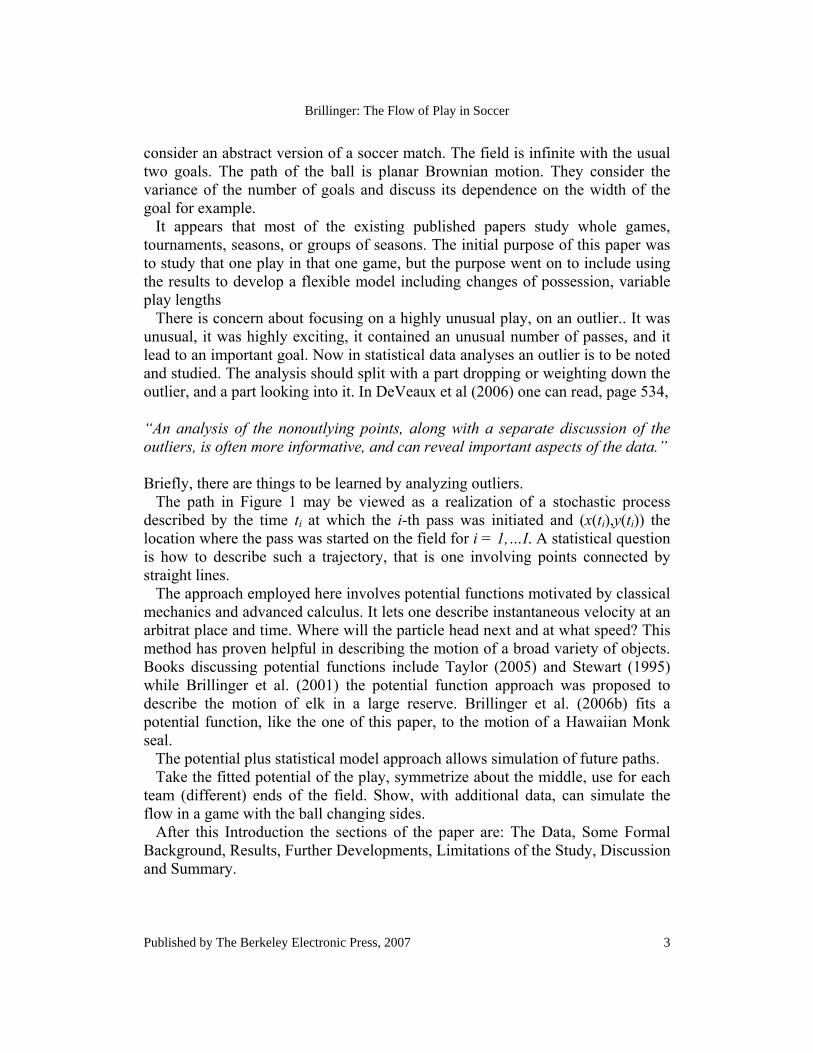
consider an abstract version of a soccer match. The field is infinite with the usual two goals. The path of the ball is planar Brownian motion. They consider the variance of the number of goals and discuss its dependence on the width of the goal for example. It appears that most of the existing published papers study whole games, tournaments, seasons, or groups of seasons. The initial purpose of this paper was to study that one play in that one game, but the purpose went on to include using the results to develop a flexible model including changes of possession, variable play lengths There is concern about focusing on a highly unusual play, on an outlier.. It was unusual, it was highly exciting, it contained an unusual number of passes, and it lead to an important goal. Now in statistical data analyses an outlier is to be noted and studied. The analysis should split with a part dropping or weighting down the outlier, and a part looking into it. In DeVeaux et al (2006) one can read, page 534, “An analysis of the nonoutlying points, along with a separate discussion of the outliers, is often more informative, and can reveal important aspects of the data.” Briefly, there are things to be learned by analyzing outliers. The path in Figure 1 may be viewed as a realization of a stochastic process described by the time ti at which the i-th pass was initiated and (x(ti),y(ti)) the location where the pass was started on the field for i = 1,…I. A statistical question is how to describe such a trajectory, that is one involving points connected by straight lines. The approach employed here involves potential functions motivated by classical mechanics and advanced calculus. It lets one describe instantaneous velocity at an arbitrat place and time. Where will the particle head next and at what speed? This method has proven helpful in describing the motion of a broad variety of objects. Books discussing potential functions include Taylor (2005) and Stewart (1995) while Brillinger et al. (2001) the potential function approach was proposed to describe the motion of elk in a large reserve. Brillinger et al. (2006b) fits a potential function, like the one of this paper, to the motion of a Hawaiian Monk seal. The potential plus statistical model approach allows simulation of future paths. Take the fitted potential of the play, symmetrize about the middle, use for each team (different) ends of the field. Show, with additional data, can simulate the flow in a game with the ball changing sides. After this Introduction the sections of the paper are: The Data, Some Formal Background, Results, Further Developments, Limitations of the Study, Discussion and Summary.

3



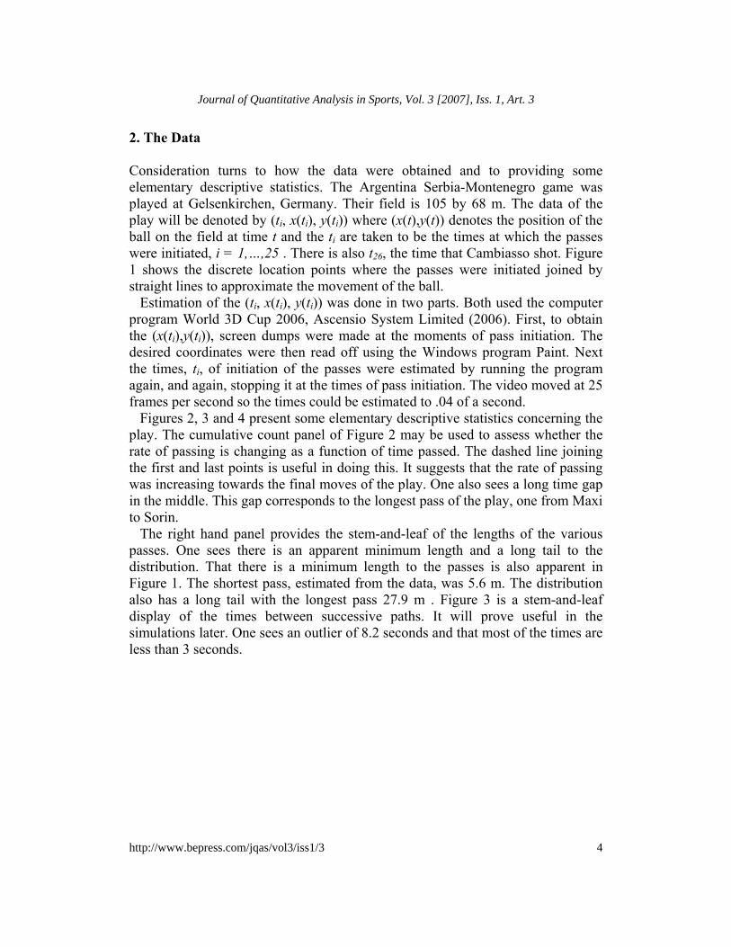
2. The Data Consideration turns to how the data were obtained and to providing some elementary descriptive statistics. The Argentina Serbia-Montenegro game was played at Gelsenkirchen, Germany. Their field is 105 by 68 m. The data of the play will be denoted by (ti, x(ti), y(ti)) where (x(t),y(t)) denotes the position of the ball on the field at time t and the ti are taken to be the times at which the passes were initiated, i = 1,…,25 . There is also t26, the time that Cambiasso shot. Figure 1 shows the discrete location points where the passes were initiated joined by straight lines to approximate the movement of the ball. Estimation of the (ti, x(ti), y(ti)) was done in two parts. Both used the computer program World 3D Cup 2006, Ascensio System Limited (2006). First, to obtain the (x(ti),y(ti)), screen dumps were made at the moments of pass initiation. The desired coordinates were then read off using the Windows program Paint. Next the times, ti, of initiation of the passes were estimated by running the program again, and again, stopping it at the times of pass initiation. The video moved at 25 frames per second so the times could be estimated to .04 of a second. Figures 2, 3 and 4 present some elementary descriptive statistics concerning the play. The cumulative count panel of Figure 2 may be used to assess whether the rate of passing is changing as a function of time passed. The dashed line joining the first and last points is useful in doing this. It suggests that the rate of passing was increasing towards the final moves of the play. One also sees a long time gap in the middle. This gap corresponds to the longest pass of the play, one from Maxi to Sorin. The right hand panel provides the stem-and-leaf of the lengths of the various passes. One sees there is an apparent minimum length and a long tail to the distribution. That there is a minimum length to the passes is also apparent in Figure 1. The shortest pass, estimated from the data, was 5.6 m. The distribution also has a long tail with the longest pass 27.9 m . Figure 3 is a stem-and-leaf display of the times between successive paths. It will prove useful in the simulations later. One sees an outlier of 8.2 seconds and that most of the times are less than 3 seconds.

4



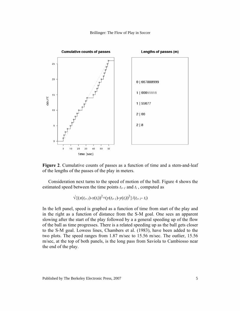
Figure 2. Cumulative counts of passes as a function of time and a stem-and-leaf of the lengths of the passes of the play in meters. Consideration next turns to the speed of motion of the ball. Figure 4 shows the estimated speed between the time points ti+1 and ti , computed as √{(x(ti+1)-x(ti))2+(y(ti+1)-y(ti))2}/(ti+1- ti) In the left panel, speed is graphed as a function of time from start of the play and in the right as a function of distance from the S-M goal. One sees an apparent slowing after the start of the play followed by a a general speeding up of the flow of the ball as time progresses. There is a related speeding up as the ball gets closer to the S-M goal. Lowess lines, Chambers et al. (1983), have been added to the two plots. The speed ranges from 1.87 m/sec to 15.56 m/sec. The outlier, 15.56 m/sec, at the top of both panels, is the long pass from Saviola to Cambiosso near the end of the play.

5



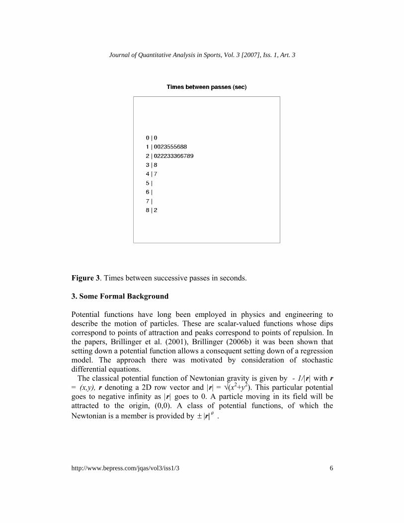
Figure 3. Times between successive passes in seconds. 3. Some Formal Background Potential functions have long been employed in physics and engineering to describe the motion of particles. These are scalar-valued functions whose dips correspond to points of attraction and peaks correspond to points of repulsion. In the papers, Brillinger et al. (2001), Brillinger (2006b) it was been shown that setting down a potential function allows a consequent setting down of a regression model. The approach there was motivated by consideration of stochastic differential equations. The classical potential function of Newtonian gravity is given by - 1/|r| with r = (x,y), r denoting a 2D row vector and |r| = √(x2+y2). This particular potential goes to negative infinity as |r| goes to 0. A particle moving in its field will be attracted to the origin, (0,0). A class of potential functions, of which the Newtonian is a member is provided by ± |r| θ .

6



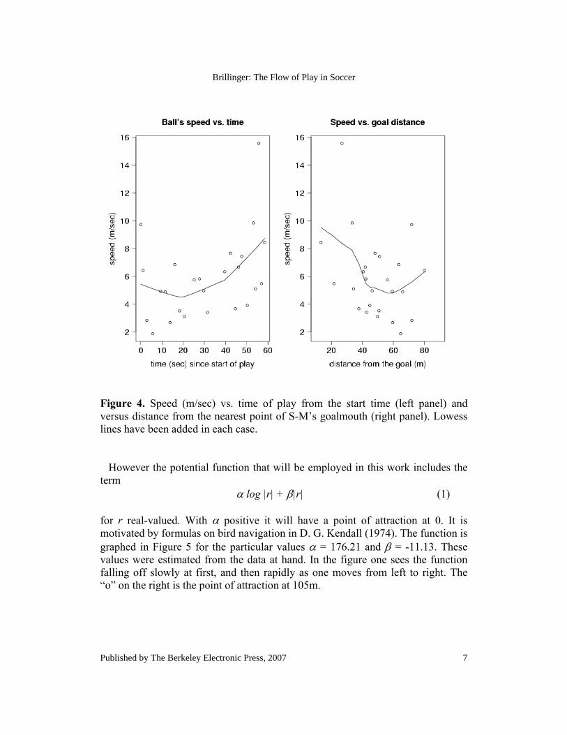
Figure 4. Speed (m/sec) vs. time of play from the start time (left panel) and versus distance from the nearest point of S-M’s goalmouth (right panel). Lowess lines have been added in each case. However the potential function that will be employed in this work includes the term α log |r| + β|r| (1) for r real-valued. With α positive it will have a point of attraction at 0. It is motivated by formulas on bird navigation in D. G. Kendall (1974). The function is graphed in Figure 5 for the particular values α = 176.21 and β = -11.13. These values were estimated from the data at hand. In the figure one sees the function falling off slowly at first, and then rapidly as one moves from left to right. The “o” on the right is the point of attraction at 105m.

7



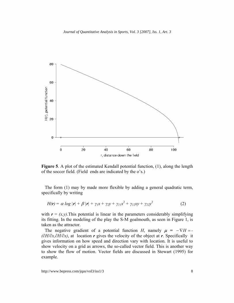
Figure 5. A plot of the estimated Kendall potential function, (1), along the length of the soccer field. (Field ends are indicated by the o’s.) The form (1) may by made more flexible by adding a general quadratic term, specifically by writing H(r) = α log |r| + β |r| + γ1x + γ2y + γ11x2 + γ12xy + γ22y2 (2) with r = (x,y).This potential is linear in the parameters considerably simplifying its fitting. In the modeling of the play the S-M goalmouth, as seen in Figure 1, is taken as the attractor. The negative gradient of a potential function H, namely µ = =∇− H -(∂H/∂x,∂H/∂x), at location r gives the velocity of the object at r. Specifically it gives information on how speed and direction vary with location. It is useful to show velocity on a grid as arrows, the so-called vector field. This is another way to show the flow of motion. Vector fields are discussed in Stewart (1995) for example.

8



Consideration now turns to setting up a specific model for this type of data. Let r(t) denote the location (x(t),y(t)) and consider the model r(ti+1)–r(ti) = µ(r(ti)) (ti+1 – ti) + iη for the changes of position with µ the gradient of a specified parametric potential function, iη a stochastic noise and the ti the times of pass initiation. In the fitting and conceptualization it proves more convenient to write (r(ti+1) – r(ti))/(ti+1 – ti) = µ(r(ti)) + iε (3) This expression makes it clear that µ has the interpretation as average velocity at r. Regarding these noise values it will be assumed, for the moment, that the x- and y-components are independent normals with mean 0 and variance σ2. Residual plots will be employed to assess whether the variance does not appear constant. Later, expression (3) will be used for simulation purposes. As expression (2) is linear in the parameters, so too will be its gradient with the implication that simple least squares may be used to estimate the parameters. The variance may be estimated by the standardized sum of the squared residuals of the fit of (3). 4. Results Figure 6 below provides the estimated potential function, ,H employing expressions (2) and (3). The redder/darker the colors the lower the value of H . The S-M goalmouth is a line of attraction. The distance |r| of (1) and (2) is taken to be shortest distance to the goal mouth from the location (x,y).

9



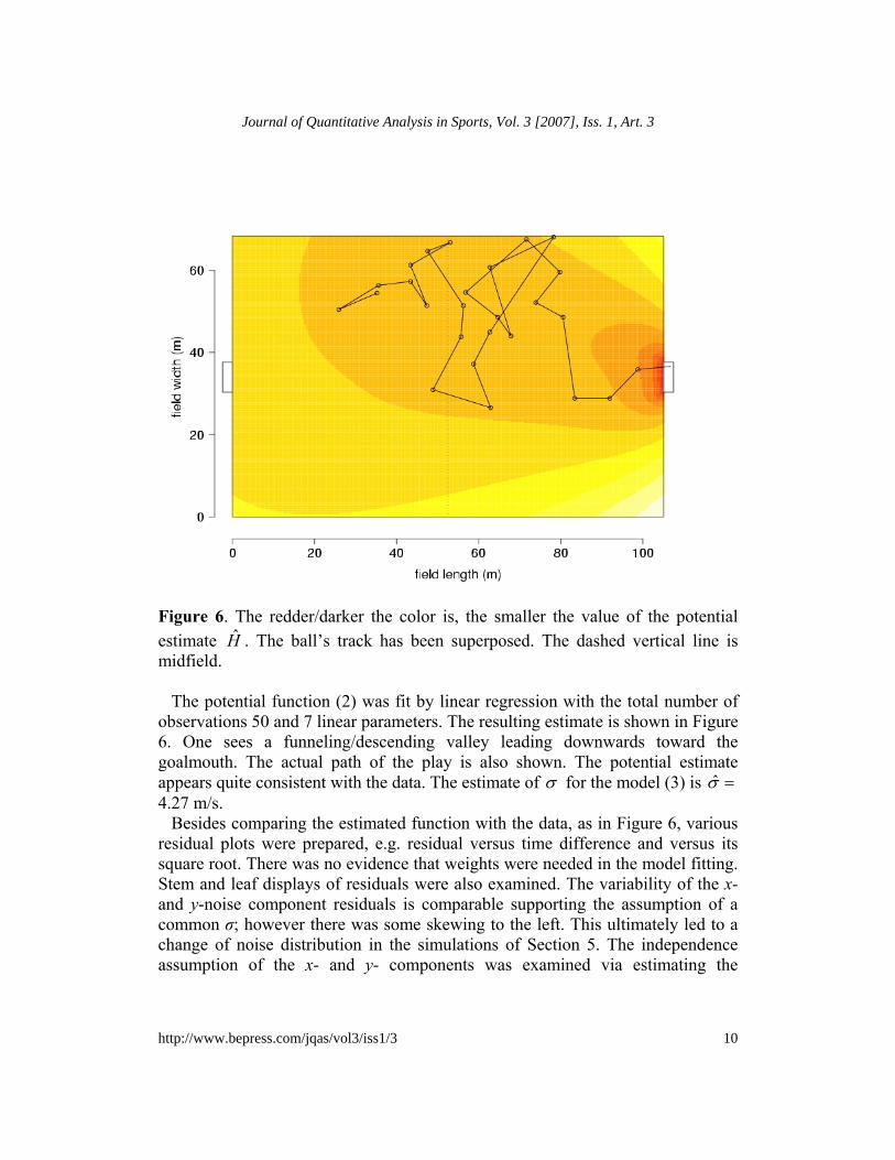
Figure 6. The redder/darker the color is, the smaller the value of the potential estimate H . The ball’s track has been superposed. The dashed vertical line is midfield. The potential function (2) was fit by linear regression with the total number of observations 50 and 7 linear parameters. The resulting estimate is shown in Figure 6. One sees a funneling/descending valley leading downwards toward the goalmouth. The actual path of the play is also shown. The potential estimate appears quite consistent with the data. The estimate of σ for the model (3) is =σ 4.27 m/s. Besides comparing the estimated function with the data, as in Figure 6, various residual plots were prepared, e.g. residual versus time difference and versus its square root. There was no evidence that weights were needed in the model fitting. Stem and leaf displays of residuals were also examined. The variability of the x- and y-noise component residuals is comparable supporting the assumption of a common σ; however there was some skewing to the left. This ultimately led to a change of noise distribution in the simulations of Section 5. The independence assumption of the x- and y- components was examined via estimating the

10



correlation coefficient and the value obtained was -.026 . The method of simulation will be employed in the next section to assess the model fit. The estimated vector field is shown in Figure 7. It provides information at the selected locations on how the average speed and direction of the ball vary with location in the field. One sees average movement from the left hand side towards the S-M goal with a speeding up as one gets closer. The value being an average, the estimated speed (arrow’s length) is small where there is back-and-forth motion in a particular area, for example in the middle of the top half of the field. One does see the to-ing and fro-ing in Figure 1.

Figure 7. The arrows represent the negative gradient, µ = -∇ H . for the locations (x,y) the arrows’ directions they provide the estimated average direction and their lengths the average speed of the motion. 5. Further Developments It would be nice to be able to fit potential functions to the data for other segments of some game. Once the data are available a way to do the fitting is clear, but the difficulty is obtaining the data. Still one can use the potential function, estimated above, for other purposes as follows.

11



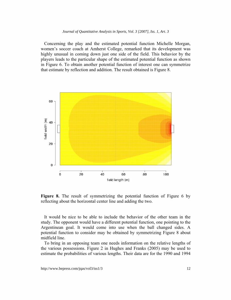
Concerning the play and the estimated potential function Michelle Morgan, women’s soccer coach at Amherst College, remarked that its development was highly unusual in coming down just one side of the field. This behavior by the players leads to the particular shape of the estimated potential function as shown in Figure 6. To obtain another potential function of interest one can symmetrize that estimate by reflection and addition. The result obtained is Figure 8.

Figure 8. The result of symmetrizing the potential function of Figure 6 by reflecting about the horizontal center line and adding the two. It would be nice to be able to include the behavior of the other team in the study. The opponent would have a different potential function, one pointing to the Argentinean goal. It would come into use when the ball changed sides. A potential function to consider may be obtained by symmetrizing Figure 8 about midfield line. To bring in an opposing team one needs information on the relative lengths of the various possessions. Figure 2 in Hughes and Franks (2005) may be used to estimate the probabilities of various lengths. Their data are for the 1990 and 1994

12



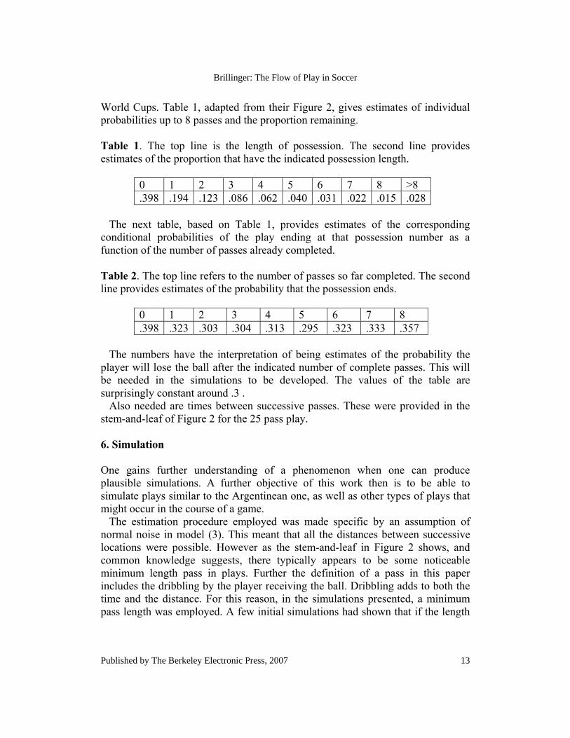
World Cups. Table 1, adapted from their Figure 2, gives estimates of individual probabilities up to 8 passes and the proportion remaining. Table 1. The top line is the length of possession. The second line provides estimates of the proportion that have the indicated possession length.

0 1 2 3 4 5 6 7 8 >8 .398 .194 .123 .086 .062 .040 .031 .022 .015 .028

The next table, based on Table 1, provides estimates of the corresponding conditional probabilities of the play ending at that possession number as a function of the number of passes already completed. Table 2. The top line refers to the number of passes so far completed. The second line provides estimates of the probability that the possession ends.

0 1 2 3 4 5 6 7 8 .398 .323 .303 .304 .313 .295 .323 .333 .357

The numbers have the interpretation of being estimates of the probability the player will lose the ball after the indicated number of complete passes. This will be needed in the simulations to be developed. The values of the table are surprisingly constant around .3 . Also needed are times between successive passes. These were provided in the stem-and-leaf of Figure 2 for the 25 pass play. 6. Simulation One gains further understanding of a phenomenon when one can produce plausible simulations. A further objective of this work then is to be able to simulate plays similar to the Argentinean one, as well as other types of plays that might occur in the course of a game. The estimation procedure employed was made specific by an assumption of normal noise in model (3). This meant that all the distances between successive locations were possible. However as the stem-and-leaf in Figure 2 shows, and common knowledge suggests, there typically appears to be some noticeable minimum length pass in plays. Further the definition of a pass in this paper includes the dribbling by the player receiving the ball. Dribbling adds to both the time and the distance. For this reason, in the simulations presented, a minimum pass length was employed. A few initial simulations had shown that if the length

13



was allowed to be very short, synthetic runs did not resemble soccer plays well. A minimum length of 5m is consequently employed in the simulations. The field’s boundaries are also an issue. Plays can end: by the ball going out of bounds, by a goal, by the ball going to an opponent, and by a referee’s whistle. There are various formal ways of dealing with boundaries when simulating realizations. The case of continuous time is reviewed in Brillinger (2003). In the present case random numbers leading to passes of length less than 5m will be rejected, as will those of passes longer than 5m that go out of bounds. One effect of this is that the noise distribution now depends on the field position in contrast to that of the model (3) which assumed common variance normal errors. The specific steps of the simulation procedure employed are: 1.The estimates α , ,β γ , σ are obtained by running a standard least squares program employing the model (3). 2. The differences between the pass times employed, the t*

i+1 – t*i , are sampled

from those of the Argentinean play, i.e. from those of Figure 3. 3. The starting field location of a simulation run is taken to be r (t1) = r(t1). 4. A tentative value generated is r (t*

i+1) = r (t*i) + µ (t*

i) (t*i+1 – t*

i) + σ Zi+1(t*i+1 – t*

i) i = 1,… with the Z’s independent bivariate standard normals. If the pass generated was less than 5m, or “the ball” goes out of bounds, then that iteration is ignored and a new Z generated. 5. A negative binomial variate is generated to determine how many passes are in a sequence. (In the simulations the probability is .2 .) 6. At this point one switches to the mirror image potential function. 7. One continues until the ball changes hands a second time. 7. Further Results The results for the first six simulation runs are provided in Figure 9. In the panels blue represents Argentina in possession of the ball and red Serbia-Montenegro. A simulation ended with either the ball changing sides a second time or a goal. As indicated at step 5 above the simulations took the conditional probability of a pass being incomplete as .2, despite .3 or so being suggested by Table 2. This was to give the plays of Figure 9 greater length for illustrative purposes. Panel 1 shows Argentina losing possession just as they enter the S-M half followed by an S-M shot. Panel 2 shows Argentina losing possession directly, and then an S-M shot. Panel 3 shows Argentina losing possession immediately followed by S-M doing the same. Panel 5 shows a representation like that of the actual goal with Argentina keeping the ball and shooting at the S-M goal..

14



In the simulations and figure one could have had the simulation run with the ball changing side more than once, but then the figures would have become cluttered. A video is called for when the ball changes hands more than twice. 8. Limitations of the Study It would be remiss not to mention some of the limitations of this study. To begin, just one play is studied. The reasons for this are twofold: the excitement of the particular play and the unavailability, just now, of other data to study. As more data become available further empirical studies may be carried out directly. In the meantime the results of the 25 play analysis can be employed to generate other potential functions, as in Section 6. Also of soccer know how can be used to set down and study other potential functions. Further it can be noted that the play studied did cover much of the field and thereby contains information on the behavior of an attacking team over a substantial part of the defending teams half. In drawing conclusions, one needs to remember that one is dealing with shots on goal, not actual goals. Shot on goals include both goals and the ball going over the crossbar. One could include goals in the simulation by having a shot become a goal with some probability, for example the 1/10 of Reep and Benjamin (1968). Also it needs to be remembered that the dribbling after receipt of the ball is included in the definition of a pass. There is measurement error, due to the discretization of the Ascensio representation. This could be studied in some detail, but it does not seem that the conclusions of the paper, for example Figures 6 and 7, are likely to change a great deal. Lastly it is to be noted that formal models are but mimics of actuality. Real people are involved. There is diving, professional fouling, anticipation, and delays of the game. In the work of the paper such effects go into the error term of expression (2).

15



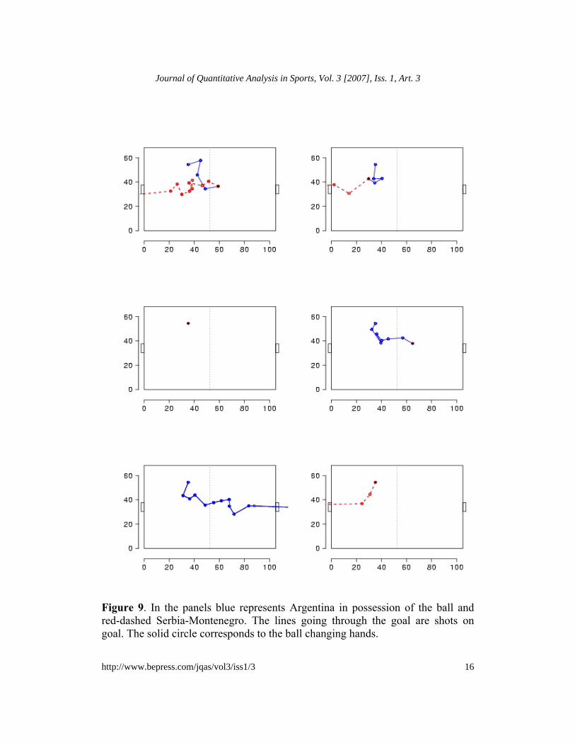
Figure 9. In the panels blue represents Argentina in possession of the ball and red-dashed Serbia-Montenegro. The lines going through the goal are shots on goal. The solid circle corresponds to the ball changing hands.

16



9. Discussion and Summary In this paper soccer has been viewed as a dynamical system with its details such as: regions of attraction, boundaries, and repulsion. The work of this paper suggests that there are analytic and conceptual advantages to employing a potential function in the description and simulation of the motion of a soccer ball. The potential is scalar-valued making it simpler to set down an expression for the instantaneous velocity as a function of location (x,y). Substantive knowledge may be employed to set down a form for a potential function and to interpret one that has been estimated. The method provides a flexible approach that is direct to invoke when other data sets come along. So much is known about the particular sport of soccer that it provides a useful test case for the potential function approach in other sports’ contexts. The approach could lead to comparative studies, classifications of plays, and further empirical studies. The approach has further led to a viable method for simulation, e.g. for bootstrapping and model appraisal. Details include: i) as an analytic formula, (2), is available for the potential function plays may be followed for any position (x,y) on the field, and ii) the potential function may change with time as in the simulations of Figure 9. One would like interpretations of the results. One can ask what might the potential function and vector field be used for and represent? Simulation use has already been emphasized. Perhaps computer-based training might be introduced to teach strategy. Perhaps the function can be used to summarize history, tactics, and even players’ intuition. Following its use in ice hockey, Thomas (2006), possession time might be another important explanatory in broader soccer studies. The possession time of the Argentinean goal was 59.6 sec. This particular goal had substantial elements of both patience and speed. References Ascensio System Limited (2006) World 3D Cup 2006 Player. Available at

http:www.footballsoftpro.com David R. Brillinger, Haiganoush K. Preisler, Alan A. Ager, and John Kie (2001)

“The Use of Potential Functions in Modelling Animal Movement” Data Analysis From Statistical Foundations, 369-386. Available at: http://www.stat.berkeley.edu/~brill/papers.html

17



David R. Brillinger (2003). “Simulating Constrained Animal Motion Using Stochastic Differential Equations.” Probability, Statistics and their Applications (Eds. K. Athreya, M. Majumdar, M. Puri and E. Waymire) Institute of Mathematical Statistics, Beachwood. Available at: http://www.stat.berkeley.edu/~brill/papers.html

David R. Brillinger (2006a) “Modelling Some Norwegian Soccer Data” Doksum

Festschrift, forthcoming. Available at: http://www.stat.berkeley.edu/~brill/papers.html

David R. Brillinger (2006b) “A Meandering Hylje”, Festschrift for Tarmo Pukkila

on His 60th Birthday (Eds. E. P. Liski, J. Isotalo, S. Puntanen, and G.P.H. Styan) Dept. of Mathematics, Statistics and Philosophy, Univ. of Tampere, Finland. Available at: http://www.stat.berkeley.edu/~brill/Papers/hylje1.pdf

John M. Chambers, William S. Cleveland, Beat Kleiner and Paul A. Tukey

(1983). Graphical Methods For Data Analysis. Duxbury, Boston. Richard D. De Veaux, Paul F. Velleman and David E. Bock (2006). Intro Stats.

Pearson, Boston. D. Karlis, and J. Ntzoufras (2003) “Analysis of Sports Data Using Bivariate

Poisson Models” The Statistician 52, 381-393. Nobuyoshi Hirotsu and Mike B. Wright (2002) “Using a Markov process model

of an Association Football Match to determine the Optimal Timing of Substitution and Tactical Decisions” Journal of the Operational Research Society: Vol. 53: No. 1, 88-96.

Nobuyoshi Hirotsu and Mike B. Wright (2006) “Modeling Tactical Changes of

Formation in Association Football as a Zero-Sum Game”, Journal of Quantitative Analysis in Sports: Vol. 2: No. 2, Article 4. Available at: http://www.bepress.com/jqas/vol2/iss2/4

M. Hughes and I. Franks (2005). “Analysis of Passing Sequences, Shots and

Goals in Soccer”. Journal of Sports Sciences 23, 509-514. David G. Kendall (1974). “Pole-seeking Brownian Motion and Bird Navigation.”

Journal of the Royal Statistical Society B: Vol. 36, 365-417.

18



S. Kozlov, J. Pitman and M. Yor (1993) “Wiener Football”. Probability Theory and its Applications 40, 530-533.

Alan J. Lee (1997). “Modelling Scores in the Premier League: Is Manchester

United Really the Best?” Chance: Vol. 10, 15-19. C. Reep and B. Benjamin (1968) “Skill and chance in association football”

Journal of the Royal Statistical Society A, 131 581- 585 James Stewart (1995) Calculus: Early Transcendentals, Third Edition. Brooks

Cole, Pacific Grove. John R. Taylor (2005) Classical Mechanics University Science, Sausalito. Andrew C. Thomas (2006) “The Impact of Puck Possession and Location on Ice

Hockey Strategy,” Journal of Quantitative Analysis in Sports: Vol. 2: No.1 Article 6. Available at: http://www.bepress.com/jqas/vol2/iss1/6

YouTube (2006a). Video of the play. Available at

http://youtube.com/watch?v=2uC5mUFye50&search=world%20cup%20006 YouTube (2006b). Video of the play. Available at:

http://www.youtube.com/watch?v=EoL8Lr9LVM4

19



A Potential Function Approach to the Flow of Play Soccer

Documents

Transcript of A Potential Function Approach to the Flow of Play Soccer