119

A possible methodology for determining the initial margin*

Marcell Béli – Kata Váradi

Our article presents a methodology for determining the initial margin requirement that complies with the EMIR regulation in effect since 2012, while also taking into account market participants’ demands and needs in connection with establishing the initial margin. The task of central counterparties that operate behind stock exchanges is to take over the counterparty risk from market participants. In order to manage the emerging risks, central counterparties operate a multilevel guarantee system, one key element of which is the initial margin. From the perspective of market participants, the main requirement is that the value of the margin reflect market developments and remain stable over time, if possible. Another requirement is that its value be determined objectively, so that market participants can easily reproduce it, i.e. it should contain as few expert decisions as possible and should be uniform with respect to all product types. We will show in the article through the example of some securities how a potential methodology is structured, and how the individual parameters can be determined in a way that satisfies the interests and the requirements of all stakeholders, i.e. regulators, market participants and the central counterparty.

Journal of Economic Literature (JEL) codes: G15, G17, G18Keywords: central counterparty, initial margin, EMIR, procyclicality

1. Introduction

The main task of central counterparties (hereinafter: CCPs) on a capital market is to ensure, in the case of potential non-performance, that the innocent party does not incur losses in the transaction as a result of the non-performance, i.e. to take over the counterparty risk from market participants. Accordingly, CCPs play a crucial role in ensuring the smooth operation of the markets. CCPs have in place a multilevel guarantee system in order to meet this requirement. For example, the

Financial and Economic Review, Vol. 16 Issue 2., June 2017, pp. 119–147.

* The views expressed in this paper are those of the author(s) and do not necessarily reflect the offical view of the Magyar Nemzeti Bank.

Marcell Béli was a market risk analyst at KELER CCP at the time the article was written.E-mail: beli.marcell@gmail.com.Kata Váradi is an associate professor at Corvinus University of Budapest and an external adviser to KELER CCP.E-mail: kata.varadi@uni-corvinus.hu.

The authors of the study are indebted to the KELER CCP for providing them with the data that form the basis for this analysis and to the staff of the Risk Management Department for their useful comments.

The manuscript was received on 25 October 2016.

DOI: http://doi.org/10.25201/FER.16.2.119147

120 Studies

Marcell Béli – Kata Váradi

CCP in Hungary, KELER KSZF Zrt. (KELER CCP) uses the following guarantee system (KELER CCP 2016):

• Basic financial collateral: this must be deposited once prior to trading in order to begin trading.

• Initial margin: the goal of this is to provide collateral for the change in the product’s price.

• Variation margin: on the day when the position is opened, it is the difference between the closing price and the trading price, while later until the settlement day it is the difference between the closing price of the current day and that of the previous day.

• Supplementary collateral: this may be collected in two cases: if a Clearing Member does not meet the minimum capital requirements, or if the size of the guarantee fund on the spot market is insufficient, and then the shortage may be collected by KELER CCP from the entity responsible for the problem.

• Additional financial collateral: this is used as collateral for individual Clearing Member risks. It is usually imposed as a sanction.

• Collective guarantee fund contribution: this is an individual and a collective guarantee element as well, since KELER CCP primarily uses the guarantee fund contribution of the guilty member, and only draws on the guarantee fund contributions of the innocent parties within the whole guarantee system at a later time.

Of these guarantee system elements, this article concentrates solely on establishing the initial margin, which aims to ensure the smooth operation of the market under normal conditions. The CCPs use various risk management models to create an adequate margin for losses incurred under normal market conditions. These models need to be set up so that they comply with the EMIR regulation1 which entered into force in 2012, and the so-called TS regulation2 which contain its details. In the case of stock exchange transactions, the requirements for risk management models are the following with respect to the margin:3

1 EMIR regulation: European Market Infrastructure Regulation (Regulation [EU] No 648/2012). Regulation (EU) No 648/2012 of the European Parliament and of the Council of 4 July 2012 on OTC derivatives, central counterparties and trade repositories. Available at: http://eur-lex.europa.eu/legal-content/EN/TXT/?uri=CELEX:32012R0648, downloaded: 8 April 2016.

2 Technical Standard (Regulation [EU] No 153/2013): Commission Delegated Regulation (EU) No 153/2013 of 19 December 2012 supplementing Regulation (EU) No 648/2012 of the European Parliament and of the Council with regard to regulatory technical standards on requirements for central counterparties. Available at: http://eur-lex.europa.eu/LexUriServ/LexUriServ.do?uri=OJ:L:2013:052:0041:0074:EN:PDF, Downloaded: 8 April 2016.

3 Article 41 of EMIR; Chapter VI of (EU) 153/2013.

121

A possible methodology for determining the initial margin

• General assumptions: the CCP’s full exposure should be covered by collaterals at least on a daily basis. In addition, the CCP should adopt models and parameters in setting its margin requirements that capture the risk characteristics of the products cleared and take into account the interval between margin collections, market liquidity and the possibility of changes over the duration of the transaction.

• Liquidation period: in the case of financial instruments other than OTC derivatives, this must be at least two working days.

• Significance level: in the case of financial instruments other than OTC derivatives, this is 99 per cent.

• Use of a portfolio-based margin requirement: the margin may only be calculated on a portfolio basis if the method used for this is prudent and robust.

• Lookback period: The margin must cover the exposures arising from the past volatility calculated on the basis of the data for the last 12 months, ensuring that the data used for calculating past volatility reflect the whole spectrum of market conditions, including stresses. Other time horizons may be used only if they entail at least as high a margin requirement as the one calculated for 12 months. If the past observation period cannot be applied, the margin parameters must be based on conservative assumptions.

• Consideration of procyclicality: The margin buffer or procyclicality buffer used must amount to at least 25 per cent of the calculated margins, and this buffer may be temporarily used in periods when the calculated margin requirements rise considerably.

However, CCPs must bear in mind not only compliance with the regulatory requirements, but also the fact that they should meet the requirements of market participants. This is because market participants expect the margin to be as stable over time as possible, while effectively reflecting market developments, and should also be easily reproduced, which means that CCPs should employ few expert decisions, i.e. the margin should be determined automatically and objectively. Another crucial factor is that CCPs use a methodology that can be applied uniformly to all products.

The margining procedure presented in this study takes into account these regulatory requirements and market demands.

The study is structured as follows: Chapter 2 presents the margin calculation methodology and the parameters, followed by an impact assessment, within the framework of which backtesting is performed in Chapter 3 and sensitivity analysis is conducted in Chapter 4, which help adequately calibrate the values of the

122 Studies

Marcell Béli – Kata Váradi

parameters used. Finally, in Chapter 5, we define stress in order to provide an objective method for establishing the lookback period in margin calculation. The article ends with a summary.

2. Margining methodology

Margin calculation is based on the appropriate choice of the degree of risk measure during the quantification of risk. In risk management systems, the most widespread measures are the Value at Risk (VaR) and the Expected Shortfall (ES) models. The choice between the two metrics can be made by weighing their advantages against each other. The advantage of the VaR over the ES is that it is easier to comprehend and backtest (Acerbi – Székely 2014; Yamai – Yoshiba 2005), elicitable4 (Ziegel 2016; Gneiting 2011), fewer data are enough for reliably calibrating the model and it is not sensitive to outliers. The advantage of the ES over the VaR is that it is coherent (Artzner et al. 1997, 1999; Pflug 2000; Frey – McNeil 2002; Acerbi – Tasche 2002), results in a stricter initial margin requirement and can take into account fat tail risk5 (Yamai – Yoshiba 2005).

Based on these advantages and drawbacks and in order to comply as fully as possible with the regulation, for CCPs it is adequate to choose the VaR methodology for determining the margin requirement, since:

• It provides a guarantee in the case of several illiquid securities for which the initial margin requirements could not be appropriately determined with the ES methodology due to the absence of data.

• It addresses the fat tail risk with other tools such as the use of expert buffers.

• Easy backtesting is important, since the regulatory authority stipulates that it should be carried out.6

• The model should not be sensitive to outliers, i.e. the initial margin requirement should be relatively stable over time.

• If the aim of the initial margin is actually to manage non-extraordinary market situations, per definition the VaR is better suited for this purpose than the ES.

• If the delta-normal method (Jorion 2007) is applied, the problem of coherency does not emerge (Jorion 2007; Szűcs 2006).

4 Elicitability means whether the result derived from the degree of risk can be verified or confirmed with other estimations.

5 Fat tail risk: the probabilities are greater than expected at the two sides of the distribution.6 Article 49 of EMIR.

123

A possible methodology for determining the initial margin

Overall, the VaR model determined with the delta-normal method can provide an adequate basis for CCPs to establish the margin. When using the delta-normal method, the VaR model requires estimates for only two parameters, namely the expected value and standard deviation, the estimation of which will be presented in the next chapter.

2.1. Parameters of the Value at Risk modelThe main goal when determining the parameters is to meet the margin requirements. Accordingly, the standard deviation parameter is determined in two ways: in an equal-weighted manner and using the exponentially weighted moving average (EWMA). Determining the equal-weighted standard deviation is insufficient because the EWMA weighting serves our above-mentioned purposes better. This is because the benefit of EWMA weighting is that it immediately jumps if a problem/stress occurs on the market, while it lets the VaR decrease under normal market conditions. The difference between the two methods of determining standard deviation is shown in the following two formulas, which also demonstrate how the EWMA fits our purposes:

The formula for equal-weighted standard deviation: σ = 1K

rt − r( )2t=1

K

∑equalσ = 1K

rt − r( )2t=1

K

∑ (1)

The formula for the EWMA standard deviation: σ = 1K

rt − r( )2t=1

K

∑EWMAσ = 1K

rt − r( )2t=1

K

∑1−λ( ) λ t−1 rt − r( )2t=1

K

∑ (2)

where rt denotes the log return on day t, r is the expected value (average) of the daily log returns, K denotes the number of days, from which the average and the standard deviation are calculated (lookback period), t denotes a given day, while λ is the parameter for exponential weighting.

The difference between the two formulas is that in the case of the equal-weighted standard deviation, the weight of each observation is 1/K, while in the case of EWMA, the older an observation, the less weight it has, thereby ensuring that new information has greater weight, i.e. its value rises in stresses, whereas if the market calms down, it lets the value of standard deviation drop more rapidly than in the case of the equal-weighted scenario. The weight of the individual observations depends on the parameter λ, called the decay factor, the value of which may be between 0 and 1. If its value is moving closer to 1, the value of the standard deviation established in this manner would converge towards the value of the equal-weighted standard deviation. The value of λ depends on two other parameters: K, i.e. the length of the lookback period and the parameter γ, which determines a tolerance level. The tolerance level must be provided because in the case of exponential weighting, past data could be observed into infinity during the estimation, since even very distant values have some minor weight, which, however,

124 Studies

Marcell Béli – Kata Váradi

can be considered negligible from the perspective of the estimation. Therefore, the data series has to be cut somewhere, and we provide a tolerance level for this, saying that the other data can be considered irrelevant from the perspective of our model. The formula of the tolerance level is the following:

γ = 1−λ( ) λ t

t=K

∞

∑ (3)

The relationship between the lookback period, the decay factor and the tolerance factor is presented in Formula 4:7

K =ln γ( )ln λ( ) (4)

It follows from the formula that the longer the lookback period, the smoother the standard deviation data series, i.e. the greater the parameter λ, thereby assigning less weight to recent data. The regulatory authority requires that the lookback period contain a stress and cover a period of at least 12 months. If both conditions are met, the VaR and thus also standard deviation are calculated based on the data for 250 trading days. In the case of a CCP, the lookback period is given, therefore the parameter that can be chosen is the tolerance level, from which the decay factor is automatically derived in Formula 4. The tolerance level was chosen to be 1 per cent, in line with EMIR’s 99 per cent significance level requirement. If the lookback period is 250 days, the tolerance level is 1 per cent, it follows that λ must be 98.17 per cent. Overall, we normally chose these parameter settings, but the lookback period may be chosen freely – since it has to be more than 250 days if there was no stress, and it cannot be applied in the case of newly introduced products either – just like the tolerance level, and therefore weighting, i.e. the value of the parameter λ, can be determined for each product/instrument.

Another element of determining the value of standard deviation is that the average of the daily log returns should be set at 0 per cent, since it can be considered close to 0 per cent, which was examined on actual data, and thus it is deemed negligible, thereby considerably reducing the computer-intensive nature of the methodology. Furthermore, due to the fact that the expected value is not taken into account while determining the standard deviation, for the sake of consistency, it will also be considered 0 per cent when determining the VaR.

With an overall λ parameter of 98.17 per cent, the standard deviation determined with the EWMA weighting and the equal-weighted standard deviation can be seen

7 RiskMetricsTM – Technical Document. J.P. Morgan /Reuters New York, 17 December 1996.

125

A possible methodology for determining the initial margin

in Figure 1 based on the log returns determined from OTP’s past exchange rate data series.

In establishing the margin, we determine the VaR both with the equal-weighted and the exponentially weighted standard deviation. The basis for the margin calculation will be the VaR that is smaller. Of course, this will depend on the parameters of the standard deviation, i.e. the basis for calculating the VaR and thus also the margin will be the smaller standard deviation. This method ensures that the reduction of the VaR follows the market to the appropriate extent, since in this case the EWMA standard deviation is smaller than the equal-weighted standard deviation, i.e. the more subdued volatility of the market will be reflected in the VaR. On the other hand, the market is not punished too much when it moves upwards, since recent events have a substantial weight in the EWMA standard deviation, so the VaR would reflect unreasonably high volatility, which would considerably increase the margin. This would be against the principles of the regulatory authority, and therefore in the case of a rising EWMA standard deviation, we employ equal weighting, assuming that the former is greater than the equal-weighted standard deviation. Overall, the VaR is determined based on Formulas 5–8, and we present how the various buffers are based on the value of the VaR, where φ denotes the liquidity buffer, θ is the

Figure 1Standard deviation with various λ parameters (OTP)

4.4

3.9

3.4

2.9

2.4

1.9

1.4

3. Ja

n. 2

011

3. M

ay 2

011

3. S

ep. 2

011

3. Ja

n. 2

012

3. M

ay 2

012

3. S

ep. 2

012

3. Ja

n. 2

013

3. M

ay 2

013

3. S

ep. 2

013

3. Ja

n. 2

014

3. M

ay 2

014

3. S

ep. 2

014

3. Ja

n. 2

015

3. M

ay 2

015

3. S

ep. 2

015

3. Ja

n. 2

016

4.4Per cent Per cent

3.9

3.4

2.9

2.4

1.9

1.4

EWMA-standard deviation (lambda = 98.17%)Equally weighted standard deviation

126 Studies

Marcell Béli – Kata Váradi

expert buffer, while π is the procyclicality buffer, and these parameters would be known to market participants, for example through publicly available disclosures.

VaRtreturn =min σ equal ⋅N−1 99%( );σ EWMA ⋅N−1 99%( )( ) (5)

VaRtprice = −Pt +Pt ⋅e T ⋅VaRt

return (6)

KSzFmargint =VaRtprice ⋅ 1+ϕ( )⋅ 1+θ( ) (7)

PROmargint =VaRtprice ⋅ 1+ϕ( )⋅ 1+θ( )⋅ 1+π( ) (8)

The aim of the liquidity buffer is to adequately manage products’ risk arising from potential illiquidity, which is not quantified by the VaR. The aim of the expert buffer is to facilitate the management of further potential risks. Such risks may arise, for example, when one margin parameter is determined for a whole product group, and margining is not performed at the product level. This may be employed, for example, on the government bond market, where one margin can be determined for each maturity, irrespective of the conditions under which the securities were issued. The procyclicality buffer is required by the regulatory authority, and its value is 25 per cent. The point of the procyclicality buffer is to facilitate the management of the effects of economic cycles in the case of margin calculation, i.e. to prevent the margin from soaring if market developments, for example a panic, would warrant this. In such cases, the regulatory authority allows CCPs to eliminate the procyclicality buffer instead of raising the margin, which would be caused by the rise in the VaR, thereby offsetting the rise in the VaR. However, the focus on the automatism and objectivity requirement warrants clearly defined criteria for the exhaustion and build-back of the procyclicality buffer, which will be presented in the next two subchapters.

2.2. Exhaustion and build-back of the procyclicality bufferThe procyclicality buffer may be exhausted if the EWMA standard deviation is greater than the equal-weighted standard deviation. Thus all in all, the treatment of the buffer would depend on the current standard deviation parameters. We decided to do this, since we believe that it is important that the current market sentiment be reflected in the establishment of the margin and the exhaustion and build-back of the buffer, i.e. whether the current period is more volatile or calm than generally in the case of the given product. This characteristic can be easily deduced from the relationship between the equal-weighted standard deviation and the EWMA-weighted standard deviation. That is why we consider it appropriate to base the treatment of the procyclicality buffer on this.

127

A possible methodology for determining the initial margin

The procyclicality buffer is not exhausted in one step, since in such a scenario the margin may plunge too much. Exhaustion of the procyclicality buffer is performed in the spirit of keeping the margin as stable as possible, even in highly volatile times. Therefore, the procyclicality buffer is exhausted by taking either the margin from the previous day (margint–1) or the value without the procyclicality buffer8 (KSzFmargint), whichever is greater, and that will be the basis for establishing the margin:

margintpro−exhaustion =max margint−1 ;KSzFmargint( ) (9)

However, this only gives us the basis for the margin if the buffer is exhausted. We have to be able to determine the build-back of the buffer, so that the procyclicality buffer is only exhausted if conditions warrant it.

The build-back of the procyclicality buffer also rests on the principle that the margin should be kept as stable as possible. If the buffer was built back in one step, the margin may move up substantially. Instead, the buffer is built back gradually, by taking either “margint

pro–exhaustion” or the margin with the procyclicality buffer (PROmargint), whichever is smaller:

margintpro−buildback =min margint

pro−exhaustion ;PROmargint( ) (10)

However, complete build-back of the procyclicality buffer must also be based on a criterion, since it may not be fully restored for a long time (for example if the VaR does not drop enough). Using the limit in reverse that we used for exhaustion – i.e. seeing when the EWMA standard deviation is smaller than the equal-weighted standard deviation – would not be practical. This could once again result in a huge spike in the margin. Therefore, the procyclicality buffer is built back gradually, in line with the EWMA standard deviation’s gradual decline below the equal-weighted standard deviation. Thus, the gradual build-back of the procyclicality buffer should be applied instead of complete build-back as long as the following condition is met:

σ = 1K

rt − r( )2t=1

K

∑EWMAσ EWMA ⋅maxmargint−1

KSzFmargint;1

⎛⎝⎜

⎞⎠⎟>σ equal (11)

If this condition is no longer met, the margin once again contains the whole procyclicality buffer. This means that this condition and the fact that the procyclicality parameter is 25 per cent determine that the procyclicality buffer is built back completely if the EWMA standard deviation drops below the equal-weighted standard deviation by 25 per cent.

8 It, however, includes other buffers, as can be seen in Formula 7.

128 Studies

Marcell Béli – Kata Váradi

2.3. Minimum marginThe precondition for restoring the procyclicality buffer can also be applied as the precondition for exhausting the buffer, since Formula 11 contains the case when the EWMA standard deviation exceeds the value of the equal-weighted standard deviation.

If we combine the formulas mentioned so far, we can determine the minimum for the margin. If we exhaust the procyclicality buffer, the minimum of the margin is “KSzFmargint”, i.e. the VaR plus the liquidity and the expert buffer, while if the procyclicality buffer is not exhausted, it is “PROmargint”, i.e. the value of “KSzFmargint” plus the procyclicality buffer. The choice between the two lower limits is determined by the values of the standard deviations compared to each other (Formula 11). The above can be incorporated into a single formula:

MINmargint = ifσ EWMA ⋅max

margint−1KSzFmargint

;1⎛⎝⎜

⎞⎠⎟>σ

⎛

⎝⎜⎞

⎠⎟;

min max margint−1 ;KSzFmargint( );PROmargint( );PROmargint

⎛

⎝

⎜⎜⎜⎜

⎞

⎠

⎟⎟⎟⎟

(12)

When determining the minimum margin, we may arrive at noninteger values. However, during this, we assume that if the margin is smaller than 1,000, we round up to whole forints, if the margin value is between HUF 1,000 and 10,000, we round up to 10, and above 10,000, we round up to 100, thereby increasing both the stability and the communicability of the margin.

2.4. Maximum margin and the margin band

However, if we set the margin to the two possible minimums each day, we would have to modify the actual margin as the minimum margin changes. The goal of the CCP, however, is to keep the margin as stable as possible, and therefore in addition to the basic expert buffer, we determine a variable expert buffer as well, aimed at providing a band (τ), within which the value of the actual margin can move above the minimum required margin. That is why we refer to this as the variable expert buffer, since its value changes each day, depending on the difference between the minimum margin and the actually applied margin. The maximum margin value is determined based on Formula 13:

MAXmargint =MINmargint ⋅ 1+τ( ) (13)

equal

MINmargint = haσ EWMA ⋅max

margint−1KSzFmargint

;1⎛⎝⎜

⎞⎠⎟>σ

⎛

⎝⎜⎞

⎠⎟;

min max margint−1 ;KSzFmargint( );PROmargint( );PROmargint

⎛

⎝

⎜⎜⎜⎜

⎞

⎠

⎟⎟⎟⎟

MINmargint = haσ EWMA ⋅max

margint−1KSzFmargint

;1⎛⎝⎜

⎞⎠⎟>σ

⎛

⎝⎜⎞

⎠⎟;

min max margint−1 ;KSzFmargint( );PROmargint( );PROmargint

⎛

⎝

⎜⎜⎜⎜

⎞

⎠

⎟⎟⎟⎟

EWMA

129

A possible methodology for determining the initial margin

The maximum margin is established by the same rounding rules as in the case of the minimum margin.

2.5. Margin value

The narrower the band between the maximum and the minimum margin, the more often the margin is modified (and the smaller the variable expert buffer), since as soon as the actual margin would reach the maximum, this value, i.e. “MAXmargint” becomes the new margin, while if it reaches the minimum, the new margin value will be the “MINmargint”. As long as it does not reach either limit, the margin’s value is not modified, as shown in Formulas 14–16:

margint = if margint−1 >MAXmargint ;MAXmargint( ) (14)

margint = if margint−1 <MINmargint ;MINmargint( ) (15)

margint = if MAXmargint >margint−1 >MINmargint ;margint−1( ) (16)

Figures 2-6 show the potential margins of the various products (one liquid and a less liquid Hungarian equity, and a foreign currency) using this method and in the context of different parameters. Figures 2–4 are based on historical OTP data: Figure 2 shows the margin if the liquidity and the expert buffers are 15 per cent, while the margin band is 25 per cent; Figure 3 shows the margin in this methodology if the margin band is 50 per cent, while Figure 4 shows the margin in this methodology if both the liquidity and the expert buffers are changed to 25 per cent, and the margin band is left unchanged. Figures 5–6 show the margin determined for Masterplast and CHF. The values for “standard deviation” and “EWMA standard deviation” can be seen on the secondary y-axis in all of the figures.

Figures 2–3 demonstrate that the wider the margin band, the less the margin fluctuates. If we wish to keep the margin of a given product as stable as possible, we can adjust it through the width of the band. If we had changed the buffers, the shape of the margin would not have changed, only its level would have risen, as seen in Figure 4.

130 Studies

Marcell Béli – Kata Váradi

Figure 2OTP’s margin I

EWMA-standard deviation (%)

Standard deviation (%)

MarginMAXmarginMINmargin

PROmarginKSzFmargin

900Per centHUF

800

700

600

500

400

300

200

100

0

26. O

ct. 2

011

26. D

ec. 2

011

26. F

eb. 2

012

26. A

pr. 2

012

26. J

une

2012

26. A

ug. 2

012

26. O

ct. 2

012

26. D

ec. 2

012

26. F

eb. 2

013

26. A

pr. 2

013

26. J

une

2013

26. A

ug. 2

013

26. O

ct. 2

013

26. D

ec. 2

013

26. F

eb. 2

014

26. A

pr. 2

014

26. J

une

2014

26. A

ug. 2

014

26. O

ct. 2

014

26. D

ec. 2

014

26. F

eb. 2

015

26. A

pr. 2

015

26. J

une

2015

26. A

ug. 2

015

26. O

ct. 2

015

26. D

ec. 2

015

8.4

7.4

6.4

5.4

4.4

3.4

2.4

1.4

Figure 3OTP’s margin II

900Per centHUF

800

700

600

500

400

300

200

100

0

EWMA-standard deviation (%)Standard deviation (%)Margin

MAXmarginMINmargin

PROmarginKSzFmargin

8.4

7.4

6.4

5.4

4.4

3.4

2.4

1.4

26. O

ct. 2

011

26. D

ec. 2

011

26. F

eb. 2

012

26. A

pr. 2

012

26. J

une

2012

26. A

ug. 2

012

26. O

ct. 2

012

26. D

ec. 2

012

26. F

eb. 2

013

26. A

pr. 2

013

26. J

une

2013

26. A

ug. 2

013

26. O

ct. 2

013

26. D

ec. 2

013

26. F

eb. 2

014

26. A

pr. 2

014

26. J

une

2014

26. A

ug. 2

014

26. O

ct. 2

014

26. D

ec. 2

014

26. F

eb. 2

015

26. A

pr. 2

015

26. J

une

2015

26. A

ug. 2

015

26. O

ct. 2

015

26. D

ec. 2

015

131

A possible methodology for determining the initial margin

Figure 4OTP’s margin III

900Per centHUF

800

700

600

500

400

300

200

100

0

EWMA-standard deviation (%)Standard deviation (%)Margin

MAXmarginMINmargin

PROmarginKSzFmargin

8.4

7.4

6.4

5.4

4.4

3.4

2.4

1.4

26. O

ct. 2

011

26. D

ec. 2

011

26. F

eb. 2

012

26. A

pr. 2

012

26. J

une

2012

26. A

ug. 2

012

26. O

ct. 2

012

26. D

ec. 2

012

26. F

eb. 2

013

26. A

pr. 2

013

26. J

une

2013

26. A

ug. 2

013

26. O

ct. 2

013

26. D

ec. 2

013

26. F

eb. 2

014

26. A

pr. 2

014

26. J

une

2014

26. A

ug. 2

014

26. O

ct. 2

014

26. D

ec. 2

014

26. F

eb. 2

015

26. A

pr. 2

015

26. J

une

2015

26. A

ug. 2

015

26. O

ct. 2

015

26. D

ec. 2

015

Figure 5Masterplast’s margin

160Per centHUF

140

120

100

80

60

40

20

0

3 Ap

r. 20

13

3. Ju

ne 2

013

3. A

ug. 2

013

3. O

ct. 2

013

3. D

ec. 2

013

3. F

eb. 2

014

3 Ap

r. 20

13

3. Ju

ne 2

013

3. A

ug. 2

013

3. O

ct. 2

013

3. D

ec. 2

013

3. F

eb. 2

014

3 Ap

r. 20

13

3. Ju

ne 2

013

3. A

ug. 2

013

3. O

ct. 2

013

3. D

ec. 2

013

3. F

eb. 2

014

6.8

5.8

4.8

3.8

2.8

1.8

EWMA-standard deviation (%)Standard deviation (%)Margin

MAXmarginMINmargin

PROmarginKSzFmargin

132 Studies

Marcell Béli – Kata Váradi

Figure 5 contains the margin for a less liquid equity, Masterplast, which, however, cannot be deemed illiquid. In this case, both the liquidity and the expert buffer are set at 25 per cent, and the margin band is 50 per cent. Based on the figure we can say that the methodology presented in this article reflects the actual market developments at the level of the margin, thereby capturing the current risks. It is also evident in this case that if the margin band had been set narrower, the margin would have reflected the actual market developments even more.

We showed how the margin is determined in the case of shares representing a liquid and a less liquid product. However, this method works and can be used for other products as well. Figure 6 shows how the margin would have developed in our methodology in the case of a foreign currency (liquidity buffer 10 per cent, expert buffer 10 per cent, margin band 25 per cent).

These figures clearly show that the margin was able to reflect the actual market developments, since the jump in the exchange rate of the Swiss franc in early 2015 was handled without unduly increasing the margin, only to the level that was necessary (based on the results of the backtesting presented later) to enable the CCP to manage the elevated risk.

Figure 6The CHF’s margin

25Per centHUF

20

15

10

5

0

25. O

ct. 2

011

25. D

ec. 2

011

25. F

eb. 2

012

25. A

pr. 2

012

25. J

une.

201

225

. Aug

. 201

225

. Oct

. 201

225

. Dec

. 201

225

. Feb

. 201

325

. Apr

. 201

325

. Jun

e. 2

013

25. A

ug. 2

013

25. O

ct. 2

013

25. D

ec. 2

013

25. F

eb. 2

014

25. A

pr. 2

014

25. J

une.

201

425

. Aug

. 201

425

. Oct

. 201

425

. Dec

. 201

425

. Feb

. 201

525

. Apr

. 201

525

. Jun

e. 2

015

25. A

ug. 2

015

25. O

ct. 2

015

25. D

ec. 2

015

25. F

eb. 2

016

7.3

5.3

6.3

4.3

3.3

2.3

1.3

0.3

EWMA-standard deviation (%)Standard deviation (%)Margin

MAXmarginMINmargin

PROmarginKSzFmargin

133

A possible methodology for determining the initial margin

Nonetheless, despite the fact that the methodology can be applied to other products as well, it must be noted that based on the unique features of other products such as their risk factor, the methodology may be modified by incorporating further parameters to take into account these special characteristics. However, this does not change the logic behind the methodology, it merely expands it. The description of these unique features and the modification of the methodology is beyond the scope of this article.

2.6. Methodology for objectively establishing the parameters – Margin groupsBased on the establishment of the margins in the previous chapter, it was demonstrated that the value of the margin depends largely on the parameters applied when establishing the buffers. These buffers are not determined on an ad-hoc basis: the products are divided into groups, and within those, the parameters are uniform by default. The buffer parameters can be determined through backtesting and sensitivity analysis. Obviously, if the backtesting results for the securities show that the values of the buffers applied to the margin group are incorrect, the parameters can be changed at the level of products/instruments in the direction of either tightening or relaxing them, i.e. the parameter settings can become unique. For example in the case of shares and foreign currencies, the classification may be as follows for KELER CCP:

Table 1Margin groups

Product group Margingroups

Equity leading;

premium (non-leading);

standard;

T-category (non-illiquid);

illiquid.

Currencies leading HUF;

leading cross;

standard HUF;

standard cross.

In the case of equities, classification may be based for example on the classification used at the Budapest Stock Exchange (hereinafter: BSE).9 The BSE classifies equities into premium, standard and T categories. CCPs should also use two additional categories, leading products and illiquid products, so that they can take into account risks to the appropriate extent. Highlighting leading products is also important because on the BSE, most of the trading is concentrated in a few products. Due

9 https://www.bet.hu/Befektetok/Reszveny-szekcio, downloaded: 8 April 2016.

134 Studies

Marcell Béli – Kata Váradi

to this concentration risk, the group of equities in which most of the trading is concentrated should be set apart from the premium category. And classifying illiquid equities into a separate group is important because their risk arising from their illiquidity is substantial. This risk should be quantified using various liquidity measures; for a CCP, one potentially appropriate indicator may be a weighted spread measure such as the Budapest Liquidity Measure (BLM)10 used by the BSE. The weighted spread measures can be determined based on the current order book in the context of various trade levels. Based on the weighted spread measure, those T category equities can be considered illiquid in the case of which the establishment of the weighted spread measure was not ensured at a specific trade level and for the given proportion of trading days. This is tantamount to the absence of a trading book for a given product on the given day that would have ensured the performance of the transactions to market participants, i.e. the market not being liquid enough.

Leading products based on trading should also be determined in the case of foreign currencies as well, in two separate groups: among forint crosses on the one hand, and among non-forint based foreign currencies on the other hand. The foreign currencies that are traded less could also be classified into the standard category in forint and non-forint groups.

Overall, in all product groups within the established margin groups, the parameters rise monotonically. For example, as we saw in the presentation of the margin methodology, the liquidity buffer was 15 per cent for OTP – assuming that it is a leading product – while the liquidity buffer for Masterplast, a standard equity, was 25 per cent.

Within most margin groups, margin calculation is performed in the manner we described in the presentation of the new methodology, only the applied parameters are different. However, in the illiquid category introduced above, the presented methodology cannot be used, since no appropriate past data series is available to the CCPs that would enable the new methodology to yield satisfactory results. Yet this problem does not only arise in the case of illiquid papers, but also during initial public offerings (IPOs). However, the discussion of this issue is also beyond the scope of this article, but it can be easily incorporated into the methodological framework using reference indices as risk factors.

10 https://www.bet.hu/portal/Kereskedesi-adatok/Adatletoltes/Budapesti_likviditasi_mertek/Budapesti_likviditasi_mertek_linkelt_tartalom, downloaded: 8 April 2016.

135

A possible methodology for determining the initial margin

3. Backtesting

Backtesting is performed in two ways for all products. First, we gauge how many times the actual daily exchange rate movements exceeded the applied margin over the past 250 trading days, and we also examine how many times the actual daily price changes exceeded the VaR value. In the case of the VaR, we do not look at VaR calculated with the equal-weighted standard deviation and the EWMA-weighted variety: we always use the smaller value in backtesting, since we also used that in establishing the margin. Accordingly, the 99 per cent requirement will probably be not met for the VaR, since we always employ the smaller value, but the figure has to be close to that if the models function well and the parameters are set correctly. In the case of the margin, the goal is to achieve an adequacy of close to 100 per cent, since the buffers used should ensure an adequacy of over 99 per cent for the margin. Based on the backtesting, the following results were obtained in the case of the products under review, over a 1-year time period:

Table 2Results of the backtesting

Adequacy

Product group Security Margin VaR (min: equal-weighted, EWMA)

Equities OTP 100.00% 98.80%

Masterplast 100.00% 99.20%

Foreign currency CHF 100.00% 100.00%

Average 100.00% 99.33%

Table 2 shows that on average, the margin was 100 per cent adequate for all the products under review, i.e. the price movement was never greater than the applied margin. And in the case of the VaR we can see that the knock-out was 0.67 per cent on average, i.e. the applied VaR calculation corresponded to 99 per cent. The results are represented graphically in Figures 7–9.

136 Studies

Marcell Béli – Kata Váradi

Figure 7Backtesting OTP

700HUFHUF

600

500

400

300

200

100

0

700

600

500

400

300

200

100

0

20. F

eb. 2

015

20. M

ar. 2

015

20. A

pr. 2

015

20. M

ay 2

015

20. J

une

2015

20. J

uly

2015

20. A

ug. 2

015

20. S

ep. 2

015

20. O

ct. 2

015

20. N

ov. 2

015

20. D

ec. 2

015

20. J

an. 2

016

20. F

eb. 2

016

Price change VaR-standard deviationVaR-EWMA-standard deviationMargin

Figure 8Backtesting Masterplast

120HUFHUF

100

80

60

40

20

0

120

100

80

60

40

20

0

2. M

ar. 2

015

2. A

pr. 2

015

2. M

ay 2

015

2. Ju

ne 2

015

2. Ju

ly 2

015

2. A

ug. 2

015

2. S

ep. 2

015

2. O

ct. 2

015

2. N

ov. 2

015

2. D

ec. 2

015

2. Ja

n. 2

016

2. F

eb. 2

016

2. M

ar. 2

016

Price change VaR-standard deviationVaR-EWMA-standard deviationMargin

137

A possible methodology for determining the initial margin

4. Sensitivity analysis

In the course of sensitivity analysis, we examine how, ceteris paribus, a change in one parameter changes the margin to be applied, and how it influences the backtesting results. Based on this, we can analyse which parameter will have the greatest influence on the margin and the backtesting results if we change the parameters to the same extent (e.g. by 1 per cent). In order to ensure the comparability of the results, the analysis was performed for the margin applied on 30 December 2015 (the last trading day in 2015) in the case of all the products under review.

However, the established margin is path-dependent as a result of the margin band, since the first day when the methodology is applied is important, as is the value of the margin for this day. Different starting and end dates may reach the minimum and the maximum of the margin band, and therefore the margin may change at different times. In order to address this path-dependency, the lookback period in the sensitivity analysis is always 250 days from 30 December 2015, and the 250 days before that is the basis for estimating the parameters. In addition, the initial margin is established in a way that on the first day MINmargin1 equals PROmargin1, while margin1 is the arithmetic mean of MINmargin1and MAXmargin1. On the other days, the margin calculation methodology described above is applied.

Figure 9Backtesting CHF

20HUFHUF

18

14

10

6

16

12

8

4

2

0

20

18

14

10

6

16

12

8

4

2

0

Price change VaR-standard deviationVaR-EWMA-standard deviationMargin

2. M

ar. 2

015

2. A

pr. 2

015

2. M

ay 2

015

2. Ju

ne 2

015

2. Ju

ly 2

015

2. A

ug. 2

015

2. S

ep. 2

015

2. O

ct. 2

015

2. N

ov. 2

015

2. D

ec. 2

015

2. Ja

n. 2

016

2. F

eb. 2

016

138 Studies

Marcell Béli – Kata Váradi

Overall, the parameters to be reviewed may be the following in the case of equities and foreign currencies:

1 VaR parameters:• significance level• liquidation period

2 Buffer parameters:• liquidity buffer• expert buffer• procyclicality buffer• margin band (variable expert buffer)

3 EWMA parameters• tolerance level

Only those parameters were included in the analysis that can be changed in the models of the CCP freely and on an expert basis. The only parameter the CCP can influence that is nonetheless not included in the sensitivity analysis is the length of the lookback period. This is because in the case of all parameters, we examine the effect of a change of +/– 1–20 per cent (not percentage points), but in the case of the lookback period such an analysis would be pointless, as the EMIR stipulates that the lookback period must be at least 250 days, including a stress period. Consequently, the default for each product in the models is 250 days. If the data series does not contain a stress period, the lookback period is extended not by one day at a time, but by a longer period (e.g. half a year). This is because the robustness of the model (and its reproducibility by market participants) would be reduced if a basic parameter of the calculation of standard deviation was changed on a daily basis. If no stress event can be observed on the market in the next half year either, the lookback period is extended by another half a year. This continues until a stress is reached. Therefore, it is pointless to conduct sensitivity analysis in the case of the lookback period, as its result will never impact experts’ decisions.

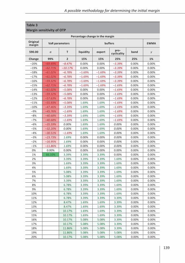
The sensitivity analysis of OTP yields the percentage changes in the margin as shown in Table 3 (the initial parameters were the following: significance level: 99 per cent; liquidation period: 2 days; liquidity buffer: 15 per cent; expert buffer: 15 per cent; procyclicality buffer: 25 per cent; margin band: 25 per cent; tolerance level: 1 per cent), and Table 4 reflects the results of the sensitivity analysis of the backtesting.

139

A possible methodology for determining the initial margin

Table 3Margin sensitivity of OTP

Percentage change in the margin

Original margin VaR parameters buffers EWMA

590.00 α T liquidity expert pro- cyclicality band γ

Change 99% 2 15% 15% 25% 25% 1%–20% –69.49% –8.47% 0.00% 0.00% –3.39% 0.00% 0.00%–19% –62.71% –10.17% 0.00% 0.00% –3.39% 0.00% 0.00%–18% –61.02% –6.78% –1.69% –1.69% –3.39% 0.00% 0.00%–17% –61.02% –6.78% –1.69% –1.69% –3.39% 0.00% 0.00%–16% –59.32% –6.78% –1.69% –1.69% –3.39% 0.00% 0.00%–15% –62.71% –6.78% –1.69% –1.69% –1.69% 0.00% 0.00%–14% –61.02% –5.08% 0.00% 0.00% –1.69% 0.00% 0.00%–13% –59.32% –5.08% 0.00% 0.00% –1.69% 0.00% 0.00%–12% –57.63% –6.78% 0.00% 0.00% –1.69% 0.00% 0.00%–11% –55.93% –5.08% 1.69% 1.69% –1.69% 0.00% 0.00%–10% –47.46% –3.39% 1.69% 1.69% –1.69% 0.00% 0.00%–9% –45.76% –1.69% 1.69% 1.69% –1.69% 0.00% 0.00%–8% –40.68% –3.39% 1.69% 1.69% –1.69% 0.00% 0.00%–7% –40.68% –1.69% 1.69% 1.69% –1.69% 0.00% 0.00%–6% –35.59% 0.00% 1.69% 1.69% 0.00% 0.00% 0.00%–5% –32.20% 0.00% 1.69% 1.69% 0.00% 0.00% 0.00%–4% –30.51% –1.69% 1.69% 1.69% 0.00% 0.00% 0.00%–3% –23.73% 1.69% 0.00% 0.00% 0.00% 0.00% 0.00%–2% –16.95% 1.69% 0.00% 0.00% 0.00% 0.00% 0.00%–1% –11.86% 1.69% 0.00% 0.00% 0.00% 0.00% 0.00%0% 0.00% 0.00% 0.00% 0.00% 0.00% 0.00% 0.00%1% 66.10% 3.39% 3.39% 3.39% 0.00% 0.00% 0.00%2% N/A 3.39% 3.39% 3.39% 1.69% 0.00% 0.00%3% N/A 1.69% 3.39% 3.39% 1.69% 0.00% 0.00%4% N/A 1.69% 3.39% 3.39% 1.69% 0.00% 0.00%5% N/A 5.08% 3.39% 3.39% 1.69% 0.00% 0.00%6% N/A 5.08% 3.39% 3.39% 1.69% 0.00% 0.00%7% N/A 3.39% 3.39% 3.39% 1.69% 0.00% 0.00%8% N/A 6.78% 3.39% 3.39% 1.69% 0.00% 0.00%9% N/A 6.78% 3.39% 3.39% 1.69% 0.00% 0.00%

10% N/A 6.78% 3.39% 3.39% 1.69% 0.00% 0.00%11% N/A 6.78% 3.39% 3.39% 3.39% 0.00% 0.00%12% N/A 8.47% 1.69% 1.69% 3.39% 0.00% 0.00%13% N/A 8.47% 1.69% 1.69% 3.39% 0.00% 0.00%14% N/A 10.17% 1.69% 1.69% 3.39% 0.00% 0.00%15% N/A 10.17% 1.69% 1.69% 3.39% 0.00% 0.00%16% N/A 10.17% 5.08% 5.08% 3.39% 0.00% 0.00%17% N/A 10.17% 5.08% 5.08% 3.39% 0.00% 0.00%18% N/A 11.86% 5.08% 5.08% 3.39% 0.00% 0.00%19% N/A 11.86% 5.08% 5.08% 5.08% 0.00% 0.00%20% N/A 10.17% 5.08% 5.08% 5.08% 0.00% 0.00%

140 Studies

Marcell Béli – Kata Váradi

Table 4Backtesting sensitivity of OTP

OTP backtesting

Original adequacy VaR parameters buffers EWMA

100.00% α T liquidity expert procyclica-lity band γ

Change 99% 2 15% 15% 25% 25% 1%

–20% 91.60% 99.60% 99.60% 99.60% 100.00% 100.00% 100.00%–19% 92.00% 99.60% 99.60% 99.60% 100.00% 100.00% 100.00%–18% 92.40% 99.60% 99.60% 99.60% 100.00% 100.00% 100.00%–17% 94.80% 99.60% 99.60% 99.60% 100.00% 100.00% 100.00%–16% 95.60% 99.60% 99.60% 99.60% 100.00% 100.00% 100.00%–15% 96.00% 99.60% 99.60% 99.60% 100.00% 100.00% 100.00%–14% 97.60% 99.60% 99.60% 99.60% 100.00% 100.00% 100.00%–13% 98.00% 99.60% 99.60% 99.60% 100.00% 100.00% 100.00%–12% 98.00% 99.60% 99.60% 99.60% 100.00% 100.00% 100.00%–11% 98.00% 99.60% 99.60% 99.60% 100.00% 100.00% 100.00%–10% 98.80% 99.60% 99.60% 99.60% 100.00% 100.00% 100.00%–9% 98.80% 99.60% 99.60% 99.60% 100.00% 100.00% 100.00%–8% 98.80% 99.60% 99.60% 99.60% 100.00% 100.00% 100.00%–7% 98.80% 99.60% 99.60% 99.60% 100.00% 100.00% 100.00%–6% 98.80% 99.60% 100.00% 100.00% 100.00% 100.00% 100.00%–5% 98.80% 99.60% 100.00% 100.00% 100.00% 100.00% 100.00%–4% 98.80% 99.60% 100.00% 100.00% 100.00% 100.00% 100.00%–3% 99.20% 99.60% 100.00% 100.00% 100.00% 100.00% 100.00%–2% 99.60% 99.60% 100.00% 100.00% 100.00% 100.00% 100.00%–1% 99.60% 100.00% 100.00% 100.00% 100.00% 100.00% 100.00%0% 100.00% 100.00% 100.00% 100.00% 100.00% 100.00% 100.00%1% 100.00% 100.00% 100.00% 100.00% 100.00% 100.00% 100.00%2% N/A 100.00% 100.00% 100.00% 100.00% 100.00% 100.00%3% N/A 100.00% 100.00% 100.00% 100.00% 100.00% 100.00%4% N/A 100.00% 100.00% 100.00% 100.00% 100.00% 100.00%5% N/A 100.00% 100.00% 100.00% 100.00% 100.00% 100.00%6% N/A 100.00% 100.00% 100.00% 100.00% 100.00% 100.00%7% N/A 100.00% 100.00% 100.00% 100.00% 100.00% 100.00%8% N/A 100.00% 100.00% 100.00% 100.00% 100.00% 100.00%9% N/A 100.00% 100.00% 100.00% 100.00% 100.00% 100.00%

10% N/A 100.00% 100.00% 100.00% 100.00% 100.00% 100.00%11% N/A 100.00% 100.00% 100.00% 100.00% 100.00% 100.00%12% N/A 100.00% 100.00% 100.00% 100.00% 100.00% 100.00%13% N/A 100.00% 100.00% 100.00% 100.00% 100.00% 100.00%14% N/A 100.00% 100.00% 100.00% 100.00% 100.00% 100.00%15% N/A 100.00% 100.00% 100.00% 100.00% 100.00% 100.00%16% N/A 100.00% 100.00% 100.00% 100.00% 100.00% 100.00%17% N/A 100.00% 100.00% 100.00% 100.00% 100.00% 100.00%18% N/A 100.00% 100.00% 100.00% 100.00% 100.00% 100.00%19% N/A 100.00% 100.00% 100.00% 100.00% 100.00% 100.00%20% N/A 100.00% 100.00% 100.00% 100.00% 100.00% 100.00%

141

A possible methodology for determining the initial margin

It can be seen in both tables (3–4) that the significance level cannot be moved in the positive direction more than 1 per cent of the 99 per cent value, otherwise the value would exceed 100 per cent; and despite the fact that the negative change of the 99 per cent is mathematically interpretable, this result does not provide important information to the CCP (just like the reduction of the liquidation period or the procyclicality buffer), since the minimum of these parameters is set by the regulators. Thus, these values were represented in smaller print, since they cannot be used for making expert decisions. All in all, the significance level could only be modified by +1 per cent, since the result was both interpretable and applicable only in this case. We had greater leeway for analysing the change in all other parameters.

We can conclude from the results that the strongest impact is exerted by the change in the significance level, while changing the margin band and the tolerance level by +/– 20 per cent did not impact the value of the margin in the case of OTP. It is interesting to note that increasing/decreasing the other parameters does not monotonically increase/decrease the margin. This is because the process of restoring the procyclicality buffer is linked to KSzFmargin, the value of which is influenced by these parameters. Furthermore, the application of the margin band makes the value of the margin path-dependent. By way of illustration, Figure 10 shows the development of the margin in the case of three different liquidity buffers. In the figure, the original 15 per cent liquidity buffer was reduced by 19 per cent, 18

Figure 10Development of the margin in the context of various liquidity buffer parameters

650HUFHUF

600

500

400

300

550

450

350

250

650

600

500

400

300

550

450

350

250

29. D

ec. 2

014

29. J

an. 2

015

28. F

eb. 2

015

31. M

ar. 2

015

30. A

pr. 2

015

30. J

une

2015

31. M

ay 2

015

31. J

uly

2015

30. S

ep. 2

015

30. N

ov. 2

015

31. A

ug. 2

015

31. O

ct. 2

015

KSzFmargin1KSzFmargin2KSzFmargin3

PROmargin1PROmargin2PROmargin3

MINmargin1MINmargin2MINmargin3

Margin1 (12.15%)Margin2 (12.30%)Margin3 (12.90%)

142 Studies

Marcell Béli – Kata Váradi

per cent and 14 per cent, respectively, and as a result the margin stayed at HUF 590 in the case of the 19 per cent and the 14 per cent reduction, while it decreased to HUF 580 on account of the 18 per cent reduction, since it took a different path.

The sensitivity analysis of the backtesting shows that currently the positive changes in the parameters do not have any effect, since backtesting originally yielded 100 per cent adequacy at the margin level, and from the perspective of the CCP, the reduction of the margin in the case of OTP only produces interesting results for the expert and the liquidity buffer. In this case we can see that if the buffers were reduced, backtesting would not have 100 per cent adequacy, since as a result of a 7 per cent reduction of any buffer (i.e. from 15 per cent to 13.59 per cent), there may have been a price movement on the market that would have exceeded the applied margin.

5. Stress

During margin calculation, it is important to define stress, since the length of the lookback period depends on whether the past 250 days included a stress. If there is no stress, the lookback period must be extended in line with the EMIR’s provisions to include a stress. As we noted in the chapter “Sensitivity analysis”, the lookback period is not changed one day at a time, but if the past 250 days did not contain a stress, it is extended by half a year.

Stress is not treated at the product level, it is defined at the level of the products that are traded the most, i.e. when these products experience stress, this automatically applies to all the other products within their product group. Currently on the Hungarian market, the following products are examined for a stress period in the lookback period: the most traded equities were considered to be the blue-chip equities, i.e. OTP, MOL, MTELEKOM and RICHTER, while in the case of foreign currencies, the EUR/HUF, USD/HUF, EUR/USD and GBP/USD are traded the most.

Nevertheless, measuring stress is not straightforward, as there is no commonly accepted methodology for this. In the literature, there are some stress indicators containing several financial indicators, based on which stress is attempted to be condensed into a single indicator, for example:

• Kansas City Financial Stress Index (KCFSI) (Hakkio – Keeton 2009)• Financial Stress Indicator of Canada (FSI) (Illing – Liu 2006)• Composite Indicator of Systemic Stress (CISS) (Holló et al 2012)• Cleveland Financial Stress Index (CFSI) (Oet et al 2015).

143

A possible methodology for determining the initial margin

However, in the case of CCPs, the use of these indicators does not appropriately show the actual stress situations as in the case of other financial institutions, since for CCPs, absolute price changes matter, they usually have a monopoly on the market, they have balanced positions, their exposures are symmetrical, they have a guarantee fund and the margin is path-dependent (Berlinger et al 2016). Consequently, a “bespoke” stress indicator should be prepared based on Berlinger et al (2016). Therefore, we propose that CCPs use their own definition and methodology for quantifying stress, rather than using stress indices that can be found on the market.

We propose the following definition for stress, taking into account the EMIR’s 99 per cent requirement for determining the margin and the steps of establishing the margin that we have presented so far: the expected shortfall (ES) at the 99 per cent significance level knocks out the initial margin. This is equivalent to looking at the VaR at 99.6 per cent (assuming that we use the delta-normal method) (Yamai – Yoshiba 2002). We use this method because the stress must refer to a rare and extreme period on the market. We believe that if the ES exceeds the margin, it may entail very significant price movements on the markets, which can be justifiably referred to as stress. In order to identify all stresses as accurately as possible, the ES calculation is not based on equal-weighted standard deviation but either the current equal-weighted or EWMA standard deviation, whichever is greater. Furthermore, the initial margin level is based on MINmargint rather than the margin, since we do not wish to take into consideration the effect of the margin band. The latter primarily serves the purpose of keeping the margin as stable as possible, it has no actual buffer-increasing and thus margin-increasing effect.

Figures 11–12 show the stresses in the individual products. In both figures, the points denote the days when stress occurred in the given product, while the coloured areas indicate the periods when the lookback period would have had to be extended, i.e. when no product from the product group experienced stress in the preceding 250 days.

144 Studies

Marcell Béli – Kata Váradi

Figure 11Stress in equities

Equities

There was no stressStress – OTP

Stress – MOLStress – Richter

Stress – Magyar Telekom

10. J

an. 2

008

10. M

ay 2

008

10. S

ep. 2

008

10. J

an. 2

009

10. M

ay 2

009

10. S

ep. 2

009

10. J

an. 2

010

10. M

ay 2

010

10. S

ep. 2

010

10. J

an. 2

011

10. M

ay 2

011

10. S

ep. 2

011

10. J

an. 2

012

10. M

ay 2

012

10. S

ep. 2

012

10. J

an. 2

013

10. M

ay 2

013

10. S

ep. 2

013

10. J

an. 2

014

10. M

ay 2

014

10. S

ep. 2

014

10. J

an. 2

015

10. M

ay 2

015

10. S

ep. 2

015

10. J

an. 2

016

Magyar Telekom

MOL

Richter

OTP

Figure 12Stress in foreign currencies

Currency pairs

There was no stressStress – EURHUF

Stress – EURUSDStress – GBPHUF

Stress – USDHUFStress – CHFHUF

10. J

an. 2

008

10. M

ay 2

008

10. S

ep. 2

008

10. J

an. 2

009

10. M

ay 2

009

10. S

ep. 2

009

10. J

an. 2

010

10. M

ay 2

010

10. S

ep. 2

010

10. J

an. 2

011

10. M

ay 2

011

10. S

ep. 2

011

10. J

an. 2

012

10. M

ay 2

012

10. S

ep. 2

012

10. J

an. 2

013

10. M

ay 2

013

10. S

ep. 2

013

10. J

an. 2

014

10. M

ay 2

014

10. S

ep. 2

014

10. J

an. 2

015

10. M

ay 2

015

10. S

ep. 2

015

10. J

an. 2

016

CHFHUF

USDHUF

GBPHUF

EURUSD

EURHUF

145

A possible methodology for determining the initial margin

In Figure 12, in the case of foreign currencies, the circled stresses do not matter from the perspective of stress in the case of CHF/HUF, because since the end of 2012, CHF/HUF was not among the most traded products.

6. Conclusions

In line with its objective, this study presents a new margining procedure, which satisfies the risk management requirements of regulators, the market and central counterparties. Our main results are the following:

a) Reflecting market developments: Determining EWMA-weighted standard deviation in addition to equal-weighted standard deviation while establishing the risk measure

b) Stable margin: The use of a margin band

c) Automatic and objective treatment of the procyclicality buffer: The exhaustion and build-back of the procyclicality buffer based on the relationship between the two standard deviation values that are weighted differently

d) Few expert decisions: A) The creation of margin groups, within which the parameters are uniform; B) Establishing the values of the liquidity and the expert buffers based on the results of the backtesting and the sensitivity analysis; C) The definition of stress for the appropriate establishment of the lookback period

Our model is based on a value-at-risk model with a 2-day liquidation period and 99 per cent significance level prepared with the delta-normal method, in which the lookback period is 250 days. Two parameters of this model, standard deviation and expected value, were determined in a way to ensure that market developments are reflected as effectively as possible, which was achieved through the establishment of the EWMA-weighted standard deviation parameter in addition to the equal-weighted standard deviation. The margin calculation was always based on the standard deviation that yields smaller values. Furthermore, the procyclicality buffer required by the regulatory authority was also exhausted and built back based on the relationship between the two different standard deviation parameters, thereby avoiding the need for hinging the treatment of the procyclicality buffer on external expert decisions. The establishment of the other buffers (the liquidity and expert buffers) was based on the results of backtesting and sensitivity analysis, also to ensure a quantifiable basis for the value of the buffers. The margin groups, within which the parameters are treated uniformly, were also set up in a way to minimise expert decisions. One parameter, the lookback period, could not be determined during backtesting and sensitivity analysis, since this would have required the definition of stress, for which we also provided a solution. Stress occurs on the market if the minimum margin is exceeded by the expected shortfall value at the

146 Studies

Marcell Béli – Kata Váradi

99 per cent significance level, where the standard deviation parameter is yielded by either the equal-weighted standard deviation or the EWMA-weighted variety, whichever is greater. The final requirement in connection with determining the margin was that – despite effectively reflecting market developments – it should be as stable as possible, which can be achieved through the use of a margin band in the methodology we have presented.

All in all, the use of this new methodology enables central counterparties to meet the legal, risk management and market participant requirements with respect to a methodology for determining the margin.

References

Acerbi, C. – Székely, B. (2014): Backtesting Expected Shortfall. MSCI working paper, 2014.

Acerbi, C. – Tasche, D. (2002): On the coherence of expected shortfall. Journal of Banking & Finance, 26(7): 1487–1503.

Artzner, P. – Delbaen, F. – Eber, J.-M. – Heath, D. (1997): Thinking coherently. Risk, 10: 68–71.

Artzner, P. – Delbaen, F. – Eber, J.M. – Heath, D. (1999): Coherent measures of risk. Mathematical Finance, 9(3): 203–228.

Berlinger, E. – Dömötör, B. – Illés, F. – Váradi, K. (2016): A tőzsdei elszámolóházak vesztesége (The loss from central clearing houses). Közgazdasági Szemle, 63(9): 993–1010.

Frey, R. – McNeil, A.J. (2002): VaR and expected shortfall in portfolios of dependent credit risks: conceptual and practical insights. Journal of Banking & Finance, 26(7): 1317–1334.

Gneiting, T. (2011): Making and evaluating point forecasts. Journal of the American Statistical Association, Vol. 106. No. 494: 746–762.

Hakkio, C.S. – Keeton, W.R. (2009): Financial stress: what is it, how can it be measured, and why does it matter? Economic Review, 94(2): 5–50.

Holló, D. – Kremer, M. – Lo Duca, M. (2012): CISS – a composite indicator of systemic stress in the financial system. Working Paper Series No. 1426 (March), European Central Bank. https://www.ecb.europa.eu/pub/pdf/scpwps/ecbwp1426.pdf?6d36165d0aa9ae601070927f3ab799fc, Downloaded: 17 August 2016.

Illing, M. – Liu, Y. (2006): Measuring financial stress in a developed country: An application to Canada. Journal of Financial Stability, 2(3): 243–265.

Jorion, P. (2007): Value at risk: the new benchmark for managing financial risk. 3rd Edition, McGraw-Hill Education; New York, p. 624.

147

A possible methodology for determining the initial margin

KeLER CCP website: https://english.kelerkszf.hu/Risk Management/Multinet/Elements of the guarantee system Downloaded: 17 August 2016.

Oet, M.V. – Dooley, J.M. – Ong, S.J. (2015): The Financial Stress Index: Identification of Systemic Risk Conditions. Risks, 3(3): 420–444.

Pflug, G.C. (2000): Some remarks on the value-at-risk and the conditional value-at-risk. In: Probabilistic constrained optimization. Springer US, pp. 272–281.

Szűcs, N.Á. (2006): VaR kritika lépésről lépésre (A step-by-step criticism of the VaR). Study prepared for the Kochmeister Competition of the Budapest Stock Exchange, Budapest.

Yamai, Y. – Yoshiba, T. (2005): Value-at-risk versus expected shortfall: A practical perspective. Journal of Banking & Finance, 29(4): 997–1015.

Ziegel, J.F. (2016): Coherence and elicitability. Mathematical Finance, 26(4), October: 901–918 (Version of Record online: 3 September 2014).