A POSITIVE NUMERICAL INTEGRATION METHOD

FOR CHEMICAL KINETIC SYSTEMS

ADRIAN SANDU∗

Abstract. Mass action chemical kinetics conserves mass and renders non-negative solutions; a good numerical

simulation would ideally produce a mass balanced, positive numerical concentration vector. Many time stepping

methods are mass conservative; however, unconditional positivity restricts the order of a traditional method to one.

The positive projection method presented in the paper ensures mass conservation and positivity. First, a numerical

approximation is computed with one step of a mass-preserving traditional scheme. If there are negative components

the nearest vector in the reaction simplex is found using a primal-dual optimization routine; this vector is shown to

better approximate the true solution. The technique works best when the underlying time-stepping scheme favors

positivity. Projected methods are able to use larger integration time steps, being more efficient then traditional

methods for systems which are unstable outside the positive quadrant.

Key words. Chemical kinetics, linear invariants, positivity, numerical time integration, primal-dual quadratic

optimization.

∗ Department of Computer Science, 205 Fisher Hall, Michigan Technological University, 1400 Townsend Drive,

Houghton, MI 49931 (asandu@mtu.edu)

1

1. Introduction. Air quality models [3, 10] solve the convection-diffusion-reaction set of

partial differential equations which model atmospheric physical and chemical processes. Usually an

operator-split approach is taken: chemical equations and convection-diffusion equations are solved

in alternative steps. In this setting the integration of chemical kinetic equations is a demanding

computational task. The chemical integration algorithm should be stable in the presence of stiffness;

ensure a modest level of accuracy, typically 1%; preserve mass (otherwise, non-physical sources and

sinks may corrupt the quality of the solution); and keep the concentrations positive. Positivity is

needed

• since concentrations are non-negative quantities;

• for stability of the chemical system;

• an operator-split solution of convection-diffusion-reaction atmospheric equations alternates

chemical integration steps with advection steps; the results of each process need to be

positive; negative concentrations from chemical integration can hurt the positivity of the

following advection step, which will perturb the next chemical step etc. leading to poor

quality results, or even unstable solutions.

An extensively used method is fixed time-step integration plus clipping. Clipping means setting

to zero the negative concentration values that appear during numerical integration of a chemical

kinetics system. It enhances stability, but adds mass to the system, therefore corrupting mass

balance.

There are numerical integration methods that preserve both mass and positivity, a well-known

example being backward Euler. However, as shown by Bolley and Crouzeix [2], positivity either

restricts the order of the method to one, or restricts the step size to impractically small values.

In this paper we try to alleviate the order and step size restrictions that come with positivity.

The idea is to obtain a mass-balanced solution using a standard integration method; if some com-

2

ponents are negative, we “project” this solution back onto the reaction simplex. This means that

we look for the mass-balanced, non-negative vector that is closest to our computed solution, and

make it the next step approximation. Lemma 4.1 shows that, in fact, this is a better approximation

of the true solution itself.

We believe the technique developed here is of interest not only for atmospheric chemistry, but

also for general kinetic mechanisms, whenever non-linearity makes negative solutions unstable. One

usually expects the step control mechanism to compensate for non-positivity and maintain stability;

this is most often the case but there is an efficiency penalty: very small time steps may be called

for. Projecting the solution back onto the reaction simplex (when needed) stabilizes the integration

process and allows larger time steps.

The paper is organized as follows. Section 2 presents the chemical kinetic problem and its

mass balance and positivity properties; the preservation of these properties by numerical schemes

is discussed in Section 3, with more details given in Appendix A. Section 4 develops the proposed

positivity-preserving algorithm. The optimization routine is briefly discussed in Section 5, and

implementation details are provided in Appendix B. A test case from stratospheric chemistry is

considered in Section 6, where different numerical results are analyzed. Finally, the findings and

conclusions of the paper are summarized in Section 7.

2. Mass action kinetics, linear invariants and positivity. Consider a chemical kinetic

system with s species y1, · · · , ys interacting in r chemical reactions,

s∑

j=1

`ij yjki−→

s∑

j=1

rij yj , i = 1, · · · , r .

Here `ij is the stoichiometric coefficient of the reactant yj in the chemical reaction i. Similarly, rik

is the stoichiometric coefficient of the product yk in reaction i and on can build the matrices of

3

stoichiometric coefficients

R = (rij)ij , L = (`ij)ij , S = R− L ∈ <s×r .(1)

Let ω(y) ∈ <r be the vector of reaction velocities,

ωi(y) = ki

s∏

j=1

(yj)`ij , i = 1, · · · , r .(2)

The time evolution of the system is governed by the “mass action kinetics” differential law

y′ = S · ω(y) , y(t0) = y0 .(3)

If e ∈ ker ST then ST e = 0, or eT S = 0, which implies that

eT y′(t) = 0 ⇐⇒ eT y(t) = const ,

that is e is a linear invariant of the system. If rank(S)=s−m, then the system admits m linearly

independent invariants, e1, · · ·, em; consider the s ×m matrix A whose columns form a basis for

the null space of ST , and the m dimensional vector b of “invariant values”, eTi y(t) = const = bi for

all i,

A = [e1|e2| · · · |em] , b = [b1, · · · , bm]T .

Then the solution satisfies

AT y(t) = b = AT y0 .

Simply stated, the existence of linear invariants ensures that mass is conserved during chemical

reactions.

Let us now separate the production reactions from the destruction ones in (3). The mass action

kinetic system (3) can be written in terms of the production terms P (y) and the destruction terms

D(y)

P (y) = Rω(y) , D(y) = diag

([Lω(y)]1

y1· · · [Lω(y)]s

ys

)

, y′ = P (y)−D(y) y .

4

The special form of the reaction speeds (2) ensures that Di(y) are polynomials in y. If at some

time moment t = τ the concentration of a certain species is zero, yi(τ) = 0, then its derivative is

nonnegative, y′i(τ) = Pi(τ) ≥ 0, which implies that

y(t0) ≥ 0 =⇒ y(t) ≥ 0 , for all t ≥ t0 .(4)

In short, the concentrations cannot become negative during chemical reactions.

Linear invariants and positivity mean that the solution of (3) remains all the time within the

reaction simplex

y(t) ∈ S for all t ≥ t0 , S ={

y ∈ <s s.t. AT y = b and yi ≥ 0 for all i}

.(5)

3. Numerical preservation of the linear invariants and of positivity. A general prin-

ciple in scientific computing says that the numerical solution must capture (as much as possible)

the qualitative behavior of the true solution. Good numerical methods for integrating chemical

reaction models (3) should therefore

• be unconditionally stable, as the system is usually stiff. This requires implicit integration

formulas;

• preserve the linear invariants. One certainly wants to avoid artificial mass creation or

destruction during integration;

• preserve solution positivity. Negative concentrations are non-physical; in addition, for

negative concetrations the whole kinetic system may become unstable.

A simple example of negative concentrations and instability is provided by Verwer et. al. [12]. The

chemical reaction

C + Ck−→ products

5

gives the following time evolution of C

C ′ = −k C2 , C(t0) = C0 =⇒ C(t) =

0 if C0 = 0 ,

(k(t− t0) + 1/C0)−1 if C0 6= 0 .

Note that if C0 > 0 the solution is bounded (0 ≤ C(t) ≤ C0) and decreases monotonically, but if

C0 < 0 the solution “explodes” in finite time, C(t)→ −∞ as t→ t0 + 1/(−C0k).

Fortunately, the most popular integration methods (Runge-Kutta, Rosenbrock and Linear Mul-

tistep) preserve exactly1 all the linear invariants of the system. Moreover, the (modified) Newton

iterations used to solve the nonlinear systems - which define implicit solutions - preserve exactly all

linear invariants during each iteration. This is briefly reminded in Appendix A. Therefore the only

errors in the linear invariants are given by roundoff. With linear-preserving integration methods

the errors in the individual species concentrations are given by the truncation errors (e.g. having a

magnitude 10−4), while the accuracy of the linear invariants is only affected by the roundoff errors

(having a much smaller magnitude, e.g. 10−14).

Positivity of the numerical solution is much harder to achieve. Bolley and Crouzeix [2] showed

that (in the linear case) ensuring positivity limits the order of the numerical method to one.

Hundsdorfer [8] proves that the implicit Euler method is positivity preserving. In practice, even

implicit Euler may produce negative values; the reason is that the implicit equations are solved

with a modified Newton process, which is halted after a finite number of iterations; while the exact

solution of implicit Euler equations is guaranteed to be non-negative, the succesive approximations

computed by (modified) Newton are not.

The most common method to avoid negative concentrations (and possible unstable behavior)

is clipping. If the solution vector has negative components, they are simply set to zero. The

problem with clipping is that it destroys the preservation of linear invariants; more exactly, the

1 If the computations are performed in infinite arithmetic precision.

6

linear invariants are corrupted by errors comparable in magnitude to the errors in the individual

components; instead of roundoff magnitude we have truncation error magnitude. The situation

is worsened by the fact that all clipping errors act in the same direction, namely increase mass;

therefore they accumulate over time and may lead to significant global errors, especially if the time

interval of interest is long. The net result is adding non-physical sources of material.

4. Solution projection method. Suppose the system (3) is solved with a linear-preserving

numerical method Φ. Let tn denote the discrete time value at nth step, yn the computed solution

and hn = tn+1 − tn the next step size. The numerical solution is represented as

yn+1 = Φ(

f, yn · · · yn−k, tn, hn · · ·hn−k+1)

.

As noted before, we consider only methods which preserve linear invariants, i.e.

AT yn+1 = AT yn = b .

Positivity is not preserved, however, and at the new moment tn+1 some numerical concentrations

may become negative

yn+1i < 0 .

We want to perform “clipping” without modifying the linear invariants. The idea is to project

the numerical solution yn+1 back onto the simplex {yi ≥ 0 for all i} ∩ {AT y = b}. The projected

value should approximate the true solution y(tn+1); therefore it has to be chosen as close as possible

to the calculated solution yn+1.

We reformulate the clipping problem as a linearly constrained, quadratic optimization problem.

Given the “computed value” yn+1 find the “projected value” zn+1 which

min1

2

∥∥∥zn+1 − yn+1

∥∥∥

2

Gsubject to AT zn+1 = b , zn+1 ≥ 0 .(6)

7

The norm used here is

‖y‖G =√

yT Gy ,

with G a positive definite matrix to be specified later.

Adjustable step ODE solvers compute the solution yn+1 together with an estimate of the

(component-wise) truncation error en+1. For example, a Runge-Kutta formula is paired with an

“embedded formula” that gives a second, lower order approximation to the solution yn+1; the

truncation error estimate is then en+1 = yn+1 − yn+1. We will denote the error estimator by

en+1 = ΦE

(

f, yn · · · yn−k, tn, hn · · ·hn−k+1)

.

The step size control is based on user-prescribed relative (rtol) and absolute (atol) error toler-

ances; the following measure of the truncation error is computed

En+1 =

√√√√1

s

s∑

i=1

(

en+1i

atol + rtol |yn+1i |

)2

.

The current value yn+1 is accepted if En+1 < 1 and rejected otherwise. It can be easily seen that

En+1 =∥∥∥en+1

∥∥∥

G(yn+1), where G(y) = diag1≤i≤s

[

1

s (atol + rtol |yi|)2

]

.

Since step control mechanism tries to keep the truncation-error norm ‖en+1‖G(yn+1) small, it is

natural to formulate the projection problem (6) in terms of the same G-norm; that is, we try to

find z in the reaction simplex (5) that the projection-error norm ‖zn+1 − yn+1‖G(yn+1) is minimal.

The computed solution yn+1 approximates the true solution y(tn+1); apparently, projection

introduces an extra error, such that ‖zn+1− y(tn+1)‖G ≤ ‖yn+1− y(tn+1)‖G + ‖zn+1− yn+1‖G. A

closer look reveals that

Lemma 4.1. The projected vector is a better (G-norm) approximation to the true solution then

is the computed vector,

∥∥∥zn+1 − y(tn+1)

∥∥∥

G≤∥∥∥yn+1 − y(tn+1)

∥∥∥

G

8

Proof. If yn+1 ≥ 0 then zn+1 = yn+1 and we have norm equality. If yn+1i < 0 for some i

consider the vectors Y = G1/2 yn+1, Z = G1/2 zn+1, W = G1/2 y(tn+1

). We have that

AT G−1/2Y = b and W ∈ S , where S ={

X : AT G−1/2X = b , X ≥ 0}

.

The problem (6) is equivalent to

min1

2‖Z − Y ‖22 subject to Z ∈ S .

Since S is a convex set, Y /∈ S, and Z is the point in S that is closest to Y , the hyperplane

perpendicular to the direction Y Z and which passes through Z separates S and Y . For any W ∈ S

the angle (Y ZW ) is larger than 90◦, therefore Y W is the largest edge in the triangle Y ZW . In

particular,

‖Y −W‖2 ≥ ‖Z −W‖2 =⇒ ‖yn+1 − y(tn+1)‖G ≥ ‖yn+1 − y(tn+1)‖G .

Schematically, one step of the method reads

yn+1 = Φ(

yn · · · yn−k, tn, hn · · ·hn−k+1)

;

G = G(yn+1) ;

if { yn+1i < 0 for some i } then

min ‖zn+1 − yn+1‖G subject to AT zn+1 = b , zn+1 ≥ 0;

yn+1 = zn+1 ;

else

yn+1 = yn+1 ;

end if

(7)

We will call this method the positive-projection method, since at each step the numerical solution

is “projected” back onto the reaction simplex (5). A direct consequence of Lemma 4.1 is that the

9

consistency order of the projection method (7) is the order of the underlying time discretization

Φ, since projection step does not increase the truncation error. The same convergence analysis

apply. In this particular sense the positive projection method (7) overcomes the order one barrier

of Bolley and Crouzeix [2].

The idea can be combined with a variable time step strategy. If en+1 is the truncation error

estimate and En+1 = ‖en+1‖G, the step is accepted for En+1 < 1 and rejected otherwise. We

check positivity only for accepted solutions, and if negative we project them. Since projection

does not increase the error norm (Lemma 4.1) the optimal value can be accepted as the new

approximation. If the optimum in (6) is not attained, but rather we are contempt with a value

zn+1 ∈ S that is “reasonably close” to yn+1, then a conservative approach makes sense; estimate

Fn+1 = ‖zn+1− yn+1‖G and check that En+1 + Fn+1 < 1; if not, reject the step and continue with

a reduced step size. This ensures that ‖zn+1 − y(tn+1)‖G < 1. Also, if the optimization algorithm

does not converge (which is possible in the presence of numerical errors, or if yn+1 is “very wrong”,

for example due to an exagerate step size) then reject the step and continue with a reduced step

size.

5. The optimization algorithm. It only remains to find a suitable way of computing zn+1,

i.e. a way to solve the quadratic minimization problem (6). Note that the reaction simplex (5)

is never empty - it contains at least the intial conditions. Therefore, the theoretical minimization

problem (6) is always feasible - we compute the minimal distance between a point and a non-empty

convex set, plus the closest point in the convex set. In principle, numerical errors may render the

problem infeasible; in this case, the whole step is rejected, and the step size reduced.

The optimization algorithm needs to have the following properties:

• Find a solution or indicate that the problem is infeasible in a finite number of steps;

• Since the number of equality constraints is much smaller than the dimension of the system,

10

m¿ s, we want to work with m-dimensional problems;

• A good starting point for the optimization routine is offered by yn+1; we have AT yn+1 = b

and the negative part(yn+1

)−is small - of the order of truncation error. Therefore, we

want to be able to initialize the optimization algorithm at an infeasible point.

The primal-dual algorithm of Goldfarb and Idnani [5] fullfills all the above criteria. This algorithm

has been adapted to our particular problem (6), which contains equality constraints, and for which

the inequality constraints have the simplest form possible.

Let K = {1, · · · , s + m} be the set of constraints of problem (6) - {1, · · · , m} are equality and

{m + 1, · · · , m + s} are inequality constraints. For a vector z with AT z = b the set of active

constraints is A = {1, · · · , m} ∪ {m + i | zi = 0}. The basic approach of the algorithm is [5]

Step 0. zn+1 = yn+1 , A = {1, · · · , m}

Step 1. Repeat until all constraints are satisfied

(a) Choose a violated constraint p ∈ K −A(

zn+1p−m < 0

)

(b) If (6) with constraints A ∪ {p} infeasible STOP;

(c) Find unnecessary constraints r ∈ A and set A ← A∪ {p} − {r};

(d) Solve (6) with equality constraints A only to get the new zn+1;

Step 2. STOP , zn+1 is the optimal solution.

(8)

A detailed presentation is given in Appendix B.

11

6. Numerical Results. Consider the basic stratospheric reaction mechanism (adapted from

nasa hsrp/aesa [9])

r1) O2 + hνk1−→ 2 O

(k1 = 2.643× 10−10 · σ3

)

r2) O + O2k2−→ O3

(k2 = 8.018× 10−17

)

r3) O3 + hνk3−→ O + O2

(k3 = 6.120× 10−04 · σ

)

r4) O + O3k4−→ 2 O2

(k4 = 1.576× 10−15

)

r5) O3 + hνk5−→ O1D + O2

(k5 = 1.070× 10−03 · σ2

)

r6) O1D + Mk6−→ O + M

(k6 = 7.110× 10−11

)

r7) O1D + O3k7−→ 2 O2

(k7 = 1.200× 10−10

)

r8) NO + O3k8−→ NO2 + O2

(k8 = 6.062× 10−15

)

r9) NO2 + Ok9−→ NO + O2

(k9 = 1.069× 10−11

)

r10) NO2 + hνk10−→ NO + O

(k10 = 1.289× 10−02 · σ

)

(9)

Here σ(t) is the normalized sunlight intensity, equal to 1 at noon at equal to 0 at nighttime.

It is easy to see that along any trajectory of the system (9) the number of oxygen and the

number of nitrogen atoms are constant,

[O1D] + [O] + 3[O3] + 2[O2] + [NO] + 2[NO2] = const , [NO] + [NO2] = const ,

therefore if we denote the concentration vector

y =

[

[O1D], [O], [O3], [O2] , [NO] , [NO2]

]T

,

the linear equality constraints have the matrix A below and a right hand side b given by the initial

conditions

AT =

1 1 3 2 1 2

0 0 0 0 1 1

, AT y(t) = AT y(t0) = b .

12

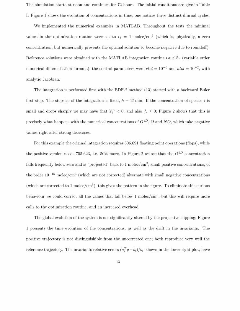
The simulation starts at noon and continues for 72 hours. The initial conditions are give in Table

I. Figure 1 shows the evolution of concentrations in time; one notices three distinct diurnal cycles.

We implemented the numerical examples in MATLAB. Throughout the tests the minimal

values in the optimization routine were set to εi = 1 molec/cm3 (which is, physically, a zero

concentration, but numerically prevents the optimal solution to become negative due to roundoff).

Reference solutions were obtained with the MATLAB integration routine ode15s (variable order

numerical differentiation formula); the control parameters were rtol = 10−6 and atol = 10−2, with

analytic Jacobian.

The integration is performed first with the BDF-2 method (13) started with a backward Euler

first step. The stepsize of the integration is fixed, h = 15 min. If the concentration of species i is

small and drops sharply we may have that Y ni < 0, and also fi ≤ 0; Figure 2 shows that this is

precisely what happens with the numerical concentrations of O1D, O and NO, which take negative

values right after strong decreases.

For this example the original integration requires 506,691 floating point operations (flops), while

the positive version needs 755,623, i.e. 50% more. In Figure 2 we see that the O1D concentration

falls frequently below zero and is “projected” back to 1 molec/cm3; small positive concentrations, of

the order 10−15 molec/cm3 (which are not corrected) alternate with small negative concentrations

(which are corrected to 1 molec/cm3); this gives the pattern in the figure. To eliminate this curious

behaviour we could correct all the values that fall below 1 molec/cm3, but this will require more

calls to the optimization routine, and an increased overhead.

The global evolution of the system is not significantly altered by the projective clipping; Figure

1 presents the time evolution of the concentrations, as well as the drift in the invariants. The

positive trajectory is not distinguishible from the uncorrected one; both reproduce very well the

reference trajectory. The invariants relative errors (aTi y−bi)/bi, shown in the lower right plot, have

13

the same order of magnitude as the double precision roundoff errors.

Next, we integrate the system with RODAS-3 (16) with a fixed step h = 15 min. We do not

give the actual solution plots, but will compare the results with other methods later on.

Finally, we integrate the system with ROS-2 (17), fixed step h = 15 min. Verwer et. al. [13, 1]

advocated the favorable positivity properties of this method. The concentration evolution is similar

to the ones obtained with BDF-2. The negative concentrations obtained are presented in Figure 3.

It is clear from the figure that this method seldom produces negative concentrations. Therefore,

the optimization routine is called fewer times and the overhead is considerably smaller. Note that,

although O1D is the only negative concentration produced, the optimization routine also adjusts

the values of NO and O (which are positive but smaller than εi = 1 molec/cm3).

The minimal concentrations throughout the trajectories are given in Table II. Note that for

ROS-2 only O1D becomes negative its minimal value −5E − 315 suggests that this is the result of

roundoff rather then algorithmic error. This conclusion is further strengthen by the results obtained

with the equivalent formulation (18), which does not produce negative values at all (the minimal

concentration of O1D along the trajectory is +5.8E − 36). In conclusion, ROS-2 favours positivity

(more details are presented in Appendix A).

The number of floating point operations needed for the standard and the positive versions of the

two codes to complete the integration are given in Table III. The conclusion is that the projective

method has to be paired with a numerical scheme that favors positivity in order to reduce the

overhead; a suitable integration method is ROS-2.

Note that in the reduced stratospheric system (9) the destruction reactions of the “possibly-

negative” species O, O1D and NO involve just 1 molecule of them; for example, the destruction

term for oxygen is −D[O][O], where D[O] does not depend on any “possibly-negative” concentration

D[O] = k2[O2] + k4[O3] + k9[NO2] ;

14

this means D[O] > 0 throughout the simuation, and for [O] < 0 the destruction term −D[O][O] > 0

(both production and destruction reactions now produce O). Since yi < 0 ⇒ fi > 0 when yi

becomes negative its derivative becomes positive, and the system pulls itself back to the quadrant

{y ≥ 0}; this auto-corrects the trajectory in case of negative values and explains why the standard

and projected trajectories are undistinguishible.

Not all chemical systems have the auto-correction property; in fact, the projection technique

is useful for systems which do not autocorrect. Consider the kinetic scheme (9) and append the

extra reaction

r11) NO + Ok11−→ NO2 (k11 = 1.0E − 8)(10)

In this case there is no auto-correction for negative values; reaction (10) will continue to destroy

NO and O even when their concentrations become negative.

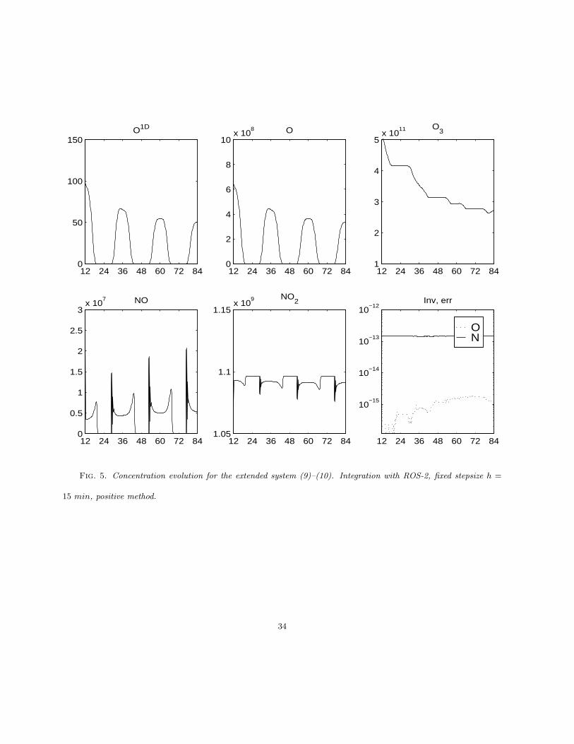
The results of integrating the extended system (9)–(10) with the fixed-step ROS-2, h = 15

min, are shown in Figure 4. The standard solution “explodes”. This behavior can be explained

as follows: at some moment the concentrations NO, O become negative reaction (10) continues at

an accelerated pace, which will trigger the accumulation of NO2, etc. In contrast, the positively-

projected solution is bounded, and is very close to the exact solution. This is shown in Figure

5.

Additional experiments (not shown here) revealed that BDF-2 with h = 15 min also has

unstable behavior. For h = 5 min both BDF-2 and ROS-2 produce stable trajectories. RODAS-3

produces stable, but very distorted trajectories for h = 15 min, and we have to go down to h = 5

min to obtain an accurate picture. Positively-projected RODAS-3 produces reasonably accurate

trajectories for h = 15 min.

An accurate solution is also produced by the variable-step ROS-2 with the modest error toler-

ances rtol = 0.01, atol = 0.01 molec/cm3; however, the chosen step-sizes are quite small (average

15

h = 3.4 min). Table IV shows the number of foating point operations needed by each method; in

particular, the variable step version is 12 times more expensive then the fixed step (h = 30 min)

positively-projected version. The positive-variable-step ROS-2 gives almost idenstical results for

rtol = 0.01; for the larger rtol = 0.1 the positive-variable-step chooses an average time step of 3.8

min, vs. 3.45 min for the standard version. In many atmospheric simulations it is customary to

impose a minimal step size, for example h ≥ hmin = 1 min. Experiments not reported here showed

that if a minimal step size is used positive projection can improve the quality of the solution.

At this point it is natural to ask whether simple clipping can stabilize the solution at a lower

cost than the full projection. Figure (6) shows the exact evolution of NO2 for the extended system

(9)–(10), the evolution with clipping and with projection, for step sizes h = 15 min and h = 30

min. Indeed, clipping stabilizes the solution, but it also introduces large errors. The clipped NO2

concentration is larger then the “exact” one and the error is increasing in time, as expected. For

the larger time step the NO2 concentration increases to 1.2×1013 molec/cm3, orders of magnitude

away from the reference solution. Large errors accumulate in the linear invariants also; for the

smaller step the accuracy drops from 10−15 to 10−1 and continues to degrade; for the larger any

meaningfull information in the invariants is lost. The NO2 values calculated with the projection

method are extremely close to the reference values; in addition the invariant errors are very small,

and remain constant in time.

Lumping does not improve the stability problem either. We integrated the lower-dimensional

equivalent system obtained by substituting [O1D] = b1 − [O]− 3[O3]− 2[O2]− [NO]− 2[NO2] and

[NO] = b2 − [NO2]. There still are negative concentrations produced, and the behavior is similar

to the one of the non-lumped system.

7. Conclusions. We have presented a technique that ensures mass conservation and positivity

for the numerical solutions of mass action kinetics initial value problems. The first numerical

16

approximation is computed with one step of a linear-invariant-preserving numerical method. If

there are negative components we find the nearest vector in the reaction simplex (5) using a primal-

dual optimization routine. The optimal vector better approximates the true solution (Lemma 4.1)

and provides the next-step numerical solution.

Standard numerical methods that guarantee positivity for any stepsize, like backward Euler,

are first order at most; higher order methods can be positive only for very small step sizes [2]. The

positive projection method overcomes this barrier; its order of consistency is given by the order of

the underlying time stepping scheme, while the solutions are guaranteed to be non-negative. In

practice the technique alleviates the step size restrictions when higher order integration methods

are used, and renders a more efficient integration process.

The projection technique has to be paired with a positivity-favourable method, for example

ROS-2 [13, 1]. Although such methods do not guarantee positivity, they seldom produce non-

positive results; this minimizes the overhead incurred by the optimization routine.

Variable step can ensure stability even when the solution becomes non-positive; sometimes very

small steps are called for. At least for the example considered, projection does not seem to improve

significantly the performance of the standard variable-step algorithm; however, improvements are

visible when a minimal step is imposed.

In air quality modeling to use fixed step integration and clipping is a popular approach; clipping,

however, constitutes a non-physical mass source which may adversely impact the quality of the

solution. Fixed step plus simplex projection ensures both positivity and mass balance. In the

example presented large values of the step size made the original solution unstable; the clipped

solution was corrupted by large errors, while the projected solution remained very similar to the

reference one. When the accuracy requirements are modest, projection may be a computationally

cheaper alternative to variable step size. In addition, in a parallel implementation of an air quality

17

model fixed step sizes lead to a better load balance and increased overall efficincy.

Some kinetic systems have the property of self-correcting negative concentrations; for them the

projection technique does not seem necessary; for kinetic systems which become unstable if some

concentrations are negative the technique is useful and improves the standard solution.

An apparent disadvantage is that one has to compute the linear invariants explicitly. The linear

invariants, however, can be automatically generated by specialized software that translates kinetic

reactions into differential equations e.g. [4].

Appendix A. Numerical integration methods. Consider the differential system (3) writ-

ten in the general form

y′(t) = f (t, y) , y(t0) = y0 .(11)

The system has the linear invariants

AT y(t) = Aty0 = b = const , AT f(t, y) = 0 , AT J = 0 (J = ∂f/∂y) .

In what follows we will denote by yn the numerical solution at n-th step (and time tn), and

h = tn+1− tn is the current time step. A linear k–step method [6, 7] is given by the general formula

yn+1 +k−2∑

i=0

αi yn−i = h

k−2∑

i=−1

βi f(

tn−i, yn−i)

.

Multiplying the relation by AT gives

AT yn+1 +k−2∑

i=0

αi AT yn−i = 0 .

If all previous approximations satisfy the invariant then the new solution also does,

AT yn−i = b , for i = 0, · · · , k − 2 =⇒ AT yn+1 = b ,

since consistency requires∑k−2

i=0 αi = −1.

18

The simplest example is the (first order) backward Euler formula,

yn+1 = yn + h f(

tn+1, yn+1)

.(12)

To solve this nonlinear equation one uses modified Newton iterations,

(I − hJ(tn, yn)) δn+1 = f(

tn+1, yn+1old

)

, yn+1new = yn+1

old − δn+1 .

Left-multiplying by AT shows preservation of linear invariants

AT J(tn, yn) = 0 , AT δn+1 = 0 , AT yn+1new = AT yn+1

old .

Another example is the second order backward differentiation formula (BDF-2)

yn+1 = Y n +2

3h f

(

tn+1, yn+1)

, Y n =4

3yn − 1

3yn−1 .(13)

For variable timesteps the coefficients change. The very first step requires both y0 and y1; the

former is given, while the latter is obtained with one backward Euler step.

An s-stage Runge-Kutta method [6] defines the solution by the formula the solution is given

by the formulas

yn+1 = yn +s∑

i=1

biki, ki = hf

tn + cih, yn +s∑

j=1

aijkj

(14)

where s and the formula coefficients bi, ci, aij are chosen for a desired order of consistency and

stability for stiff problems. Multypling the definition by AT gives

AT ki = 0 , AT yn+1 = AT yn ,

which shows that linear invariants are preserved during each step.

An s-stage Rosenbrock method [7] is usually defined for autonomous systems; the solution is

given by the formulas

yn+1 = yn +s∑

i=1

biki, ki = hf

yn +i−1∑

j=1

αijkj

+ hJi∑

j=1

γijkj ,(15)

19

where s and the formula coefficients bi, αij and γij give the order of consistency and the stability

properties. Again, multypling the definition by AT shows the preservation of the linear invariants,

AT ki = 0 , AT yn+1 = AT yn .

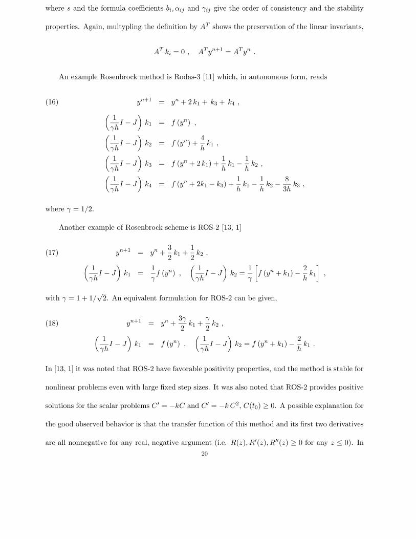
An example Rosenbrock method is Rodas-3 [11] which, in autonomous form, reads

yn+1 = yn + 2 k1 + k3 + k4 ,(16)

(1

γhI − J

)

k1 = f (yn) ,

(1

γhI − J

)

k2 = f (yn) +4

hk1 ,

(1

γhI − J

)

k3 = f (yn + 2 k1) +1

hk1 −

1

hk2 ,

(1

γhI − J

)

k4 = f (yn + 2k1 − k3) +1

hk1 −

1

hk2 −

8

3hk3 ,

where γ = 1/2.

Another example of Rosenbrock scheme is ROS-2 [13, 1]

yn+1 = yn +3

2k1 +

1

2k2 ,(17)

(1

γhI − J

)

k1 =1

γf (yn) ,

(1

γhI − J

)

k2 =1

γ

[

f (yn + k1)−2

hk1

]

,

with γ = 1 + 1/√

2. An equivalent formulation for ROS-2 can be given,

yn+1 = yn +3γ

2k1 +

γ

2k2 ,(18)

(1

γhI − J

)

k1 = f (yn) ,

(1

γhI − J

)

k2 = f (yn + k1)−2

hk1 .

In [13, 1] it was noted that ROS-2 have favorable positivity properties, and the method is stable for

nonlinear problems even with large fixed step sizes. It was also noted that ROS-2 provides positive

solutions for the scalar problems C ′ = −kC and C ′ = −k C2, C(t0) ≥ 0. A possible explanation for

the good observed behavior is that the transfer function of this method and its first two derivatives

are all nonnegative for any real, negative argument (i.e. R(z), R′(z), R′′(z) ≥ 0 for any z ≤ 0). In

20

the view of the theory developed in [2] this might reduce the the negative values and have a good

influence on the positivity of solutions.

Appendix B. The optimization algorithm. Consider the optimization problem (6), refor-

mulated as

min1

2zT Gz − yT Gz subject to AT z = b , z ≥ ε .(19)

The problem has m equality constraints (aTi z = bi, i = 1 · · ·m, where ai is the ith column of A)

and s inequality constraints (zi ≥ εi for i = 1 · · · s). The entries εi > 0 are small positive numbers;

their role is to keep zi ≥ 0 even when the computation is corrupted by roundoff. We assume that

• AT has full row rank, and that

• AT y = b (y satisfies the equality constraints).

The original algorithm of Goldfarb and Idnani is presented in [5]. We modified this algorithm

in order to

• accomodate the equality constraints AT y = b at all times, given that the starting point

satisfies them;

• take advantage of the diagonal form of G;

• take advantage of the special form of inequality constraints, zi ≥ εi;

The algorithm of Goldfarb and Idnani preserves at all times dual feasibility. The algorithm is

started from the unconstrained optimum z = y, which violates primal inequality constraints. Let

K = {1, · · · , s + m} be the set of constraint indices. For a vector z with AT z = b the set of

active constraints is A = {1, · · · , m} ∪ {m + i | zi = εi}; we will denote by q the number of active

constraints. Let N ne the matrix of normal vectors of active constraints; for example, if zi = ei

and zj = ej (q = m + 2) this matrix is

N = [a1| · · · |am|ei|ej ] ∈ <s×q .

21

Here and below ei is the unit vector with entry i equal to 1 and all other entries equal to 0. The

active constraints are expressed as

NT z =

b

0

}m

}2.

Consider N∗, the generalized inverse of N in the space of scaled variables Z = G1/2z, and the

reduced inverse Hessian operator H

N∗ =(

NT G−1N)−1

NT G−1 , H = G−1 −G−1N(

NT G−1N)−1

NT G−1 .

At each step the algorithm looks for a violated inequality constraint zp < εp. A step of the form

z+ = z + tHep(20)

will preserve all the active constraints, NT H = 0 =⇒ NT z+ = NT z. The step (20) can move the

current vector toward satisfying the constraint. We have

z+p = eT

p z+ = eTp z + teT

p Hep = zp + tHp,p

and if Hp,p > 0 we can choose t such that z+p = εp. This becomes a new active constraint and is

added to the set, N ← [N |ep].

If z is the optimum solution with respect to the given set of active constraints, the Lagrange

multipliers satisfy

λ(y) = N∗G(z − y) .

The multipliers corresponding to inequality constraints have to be non-negative, if not, the active

constraint corresponding to a negative multiplier is removed (this means that zk = εk is not optimal,

and we remove the constraint, allowing zk > εk).

22

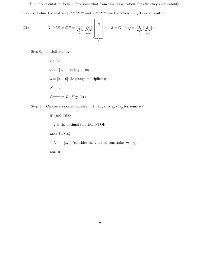
The implementation form differs somewhat from this presentation, for efficiency and stability

reasons. Define the matrices R ∈ <q×q and J ∈ <s×s via the following QR decomposition:

G−1/2N = QR = [ Q1︸︷︷︸

q

| Q2︸︷︷︸

s−q

]

R

0

︸ ︷︷ ︸

q

, J = G−1/2Q = [ J1︸︷︷︸

q

| J2︸︷︷︸

s−q

] .(21)

Step 0. Initializations.

z ← y;

A ← {1, · · · , m}; q ← m;

λ = [0 · · · 0] (Lagrange multipliers);

N ← A;

Compute R, J by (21).

Step 1. Choose a violated constraint (if any). Is zp < εp for some p ?

if {no} then

z is the optimal solution. STOP

else {if yes}

λ+ ← [λ, 0] (consider the violated constraint m + p)

end if

23

Step 2.

(a) Determine primal and dual step directions

δprimal = J(1 : s, q + 1 : s) · J(p, q + 1 : s)T

R(1 : q, 1 : q) · δdual = J(p, 1 : q)T (triangular system)

(b) Max dual step length (which maintains dual feasibility)

if { δdual ≤ 0 or q = m } then

τdual =∞

else

τdual = minj=m+1:q; δdualj

>0

{

λ+j /δdual

j

}

= λ+k /δdual

k

end if

Primal step length (which makes zp = εp)

if { δprimal = 0 } then

τprimal =∞

else

τprimal = (εp − zp)/δprimalp

end if

Step length

t = min(

τprimal, τdual)

24

Step 3.

(a) Check Infeasibility

If { (τprimal =∞) and (τdual =∞) } then

The problem is infeasible. STOP.

end if

(b) Primal Infeasible, step in dual space only

if { τprimal =∞ (Primal Infeasible) } then

λ+ ← λ+ + t[−δdual, 1]

Drop k −mth inequality constraint:

A ← A\{k}; q ← q − 1

Update R, J for newly dropped constraint

Go to Step 2(a).

end if

(c) Step in both primal and dual space

z ← z + t δprimal

λ+ ← λ+ + t [−δdual, 1]

if { t = τprimal (Full Step) } then

λ← λ+

Add pth inequality constraint:

A ← A∪ {m + p}, q ← q + 1;

Update R, J for newly added constraint;

Go to Step 1.

25

else if { t = τdual (Partial Step) } then

Drop k −mth inequality constraint:

A ← A\{k}; q ← q − 1

Update R, J for newly dropped constraint;

Go to Step 2(a).

end if

When a constraint is added, the matrices R and J are modified to accomodate it; for clarity,

in what follows the updated versions will be marked by the superscript (+). Adding the active

constraint {zp = ep} leads to the following changes.

d = (J(p, :))T =

d1

d2

}q

}s− q

U = Householder reflector s.t. Ud =

d1

σ

0

}q

}1

}s− q − 1

R+ ←

R d1

0 σ

∈ <(q+1)×(q+1)

J+ ← [ J1︸︷︷︸

q

| J2UT

︸ ︷︷ ︸

s−q

] = [ J+1

︸︷︷︸

q+1

| J+2

︸︷︷︸

s−q−1

]

When a constant is dropped, the matrices R and J are updated; for clarity, we marked the

updated versions by the superscript (−) . Dropping the active constraint {z` = e`} means deleting

the k = m + `th constraint.

R =

R1 r1k S

0 r2k T

=⇒ R =

R1 S

0 T

Delete the kth

column of R

26

U T =

R2

0

(T Hessenberg, compute easily its QR decomposition)

R− ←

R1 S

0 R2

∈ <(q−1)×(q−1)

J = [ J1︸︷︷︸

q

| J2︸︷︷︸

s−q

] = [ Ja1

︸︷︷︸

`−1

| Jb1

︸︷︷︸

q−`+1

| J2︸︷︷︸

s−q

] ;

J− ← [ Ja1

︸︷︷︸

`−1

| Jb1 UT

︸ ︷︷ ︸

q−`+1

| Jc︸︷︷︸

s−q

] = [ J−1

︸︷︷︸

q−1

| J−2

︸︷︷︸

s−q+1

]

To compute quantities of the form J2UT , Jb

1 UT note that U is a composition of Householder

reflectors, U = Un · · ·U1; they are applied in succession to the rows of J2, J2UT = (U1 · · ·UnJT

2 )T .

Acknowledgements. I thank Mihai Anitescu for a fruitful discussion regarding quadratic

optimization algorithms and the approximation properties of the solution.

REFERENCES

[1] Blom, J.G.; Verwer, J.; A comparison of integration methods for atmospheric transport-chemistry problems.

Modeling, Analysis and Simulations report MAS-R9910, CWI, Amsterdam, April 1999.

[2] Bolley, C.; Crouzeix, M.; Conservation de la positivite lors de la discretization des problemes d’evolution

parabolique. R.A.I.R.O. Numerical Analysis, 12(3):237–245, 1978.

[3] Carmichael, G.R.; Peters, L.K.; Kitada, T.; A second generation model for regional-scale transport/ chemistry/

deposition. Atmos. Env. 1986, 20, 173–188.

[4] Damian-Iordache, V.; Sandu, A.; Damian-Iordache, M.; Carmichael, G.R.; Potra, F.A.; KPP - A symbolic

preprocessor for chemistry kinetics - User’s guide. Technical report, The University of Iowa, Iowa City, IA

52246, 1995.

[5] Goldfarb, D.; Idnani, A., A numerically stable dual method for solving strictly convex quadratic programs.

Math. Prog. 1983, 27, 1–33.

[6] Hairer, E.; Norsett, S.P.; Wanner, G.; Solving Ordinary Differential Equations I. Nonstiff Problems. Springer-

Verlag, Berlin, 1993.

27

[7] Hairer, E.; Wanner, G.; Solving Ordinary Differential Equations II. Stiff and Differential-Algebraic Problems.

Springer-Verlag, Berlin, 1991.

[8] Hundsdorfer, W.; Numerical solution of advection-diffusion-reaction equations. Technical report, Department

of Numerical Mathematics, CWI, Amsterdam, 1996.

[9] Kinnison, D.E.; NASA HSRP/AESA stratospheric models intercomparison. NASA ftp site, contact kinni-

son1@llnl.gov.

[10] Sandu, A.; Numerical aspects of air quality modeling. Ph.D. Thesis, Applied Mathematical and Computational

Sciences, The University of Iowa, 1997.

[11] Sandu, A.; Blom, J.G.; Spee, E.; Verwer, J.; Potra, F.A.; Carmichael, G.R.; Benchmarking stiff ODE solvers

for atmospheric chemistry equations II - Rosenbrock Solvers. Report on Computational Mathematics 90,

The University of Iowa, Department of Mathematics, Iowa City, July 1996.

[12] Verwer, J.G.; Hunsdorfer, W.; Blom, J.G.; Numerical time integration of air pollution models. APMS’98,

Paris:France, October 1998.

[13] Verwer, J.; Spee, E.J.; Blom, J.G.; Hunsdorfer, W.; A second order Rosenbrock method applied to photochemical

dispersion problems. SIAM J. Sci. Comp., to appear, 1999.

28

Figure captions

Fig. 1. Concentration evolution for BDF-2 integration, h = 15 min; there is virtually no differ-

ence between the standard and the positively-projected solutions. The lower right plot shows relative

errors in the invariants, (aTi y − bi)/bi.

Fig. 2. Zoom in on concentration evolution with BDF-2, fixed h = 15min. Upper figure shows the

original solution, and lower figure shows the positively-projected solution.

Fig. 3. Zoom in on concentration evolution with ROS-2, fixed h = 15min. Upper figure shows the

original solution, and lower figure shows the projected solution.

Fig. 4. Concentration evolution for the extended system (9)–(10). Integration with ROS-2, fixed

stepsize h = 15 min, standard vs. positive methods. Note the unstable behavior of the standard

solution.

Fig. 5. Concentration evolution for the extended system (9)–(10). Integration with ROS-2, fixed

stepsize h = 15 min, positive method.

Fig. 6. NO2 concentration for the extended system (9)–(10) integrated with ROS-2, fixed stepsizes

h = 15 min and h = 30 min. The projection solution is very close to the reference one, while

clipping introduces errors which accumulate in time. For the larger step all meaningful information

is lost.

29

12 24 36 48 60 72 840

50

100

150O1D

Con

c. [m

olec

/cm

3 ]

12 24 36 48 60 72 840

2

4

6

8

10x 10

8 O

12 24 36 48 60 72 845

5.5

6

6.5

7

7.5

8x 10

11 O3

12 24 36 48 60 72 840

2

4

6

8

10

12x 10

8 NO

Time [hours]

Con

c. [m

olec

/cm

3 ]

12 24 36 48 60 72 840

2

4

6

8

10

12x 10

8 NO2

Time [hours]12 24 36 48 60 72 84

10−15

10−14

10−13

Invariant rel. errors

Time [hours]

StandardPositive

ON

Fig. 1. Concentration evolution for BDF-2 integration, h = 15 min; there is virtually no difference between

the standard and the positively-projected solutions. The lower right plot shows relative errors in the invariants,

(aTi y − bi)/bi.

30

20 40 60 80−2

−1

0

1

2x 10

−9 O1D

Con

c. [m

olec

/cm

3 ]

20 40 60 80−3

−2

−1

0

1

2

3O

20 40 60 80−5

0

5x 10

6 NO

20 40 60 80−3

−2

−1

0

1

2

3O1D

Time [hours]

Con

c. [m

olec

/cm

3 ]

20 40 60 80−3

−2

−1

0

1

2

3O

Time [hours]20 40 60 80

−3

−2

−1

0

1

2

3NO

Time [hours]

Fig. 2. Zoom in on concentration evolution with BDF-2, fixed h = 15min. Upper figure shows the original

solution, and lower figure shows the positively-projected solution.

31

20 40 60 80−2

−1

0

1

2x 10

−11 O1D

Con

c. [m

olec

/cm

3 ]

20 40 60 80−2000

−1000

0

1000

2000O

20 40 60 80−3

−2

−1

0

1

2

3x 10

6 NO

20 40 60 80−3

−2

−1

0

1

2

3O1D

Time [hours]

Con

c. [m

olec

/cm

3 ]

20 40 60 80−3

−2

−1

0

1

2

3O

Time [hours]20 40 60 80

−3

−2

−1

0

1

2

3NO

Time [hours]

Fig. 3. Zoom in on concentration evolution with ROS-2, fixed h = 15min. Upper figure shows the original

solution, and lower figure shows the projected solution.

32

12 48 84−20

−15

−10

−5

0

5x 10

62 O1D

Con

c. [m

olec

/cm

3 ]

12 48 84−2.5

−2

−1.5

−1

−0.5

0

0.5x 10

70 O

12 48 84−2

0

2

4

6

8

10

12x 10

73 O3

12 48 84−12

−10

−8

−6

−4

−2

0

2x 10

72 NO

Time [hours]

Con

c. [m

olec

/cm

3 ]

12 48 840

1

2

3

4

5

6x 10

72 NO2

Time [hours]

StandardProjectionStabilization

Fig. 4. Concentration evolution for the extended system (9)–(10). Integration with ROS-2, fixed stepsize h =

15 min, standard vs. positive methods. Note the unstable behavior of the standard solution.

33

12 24 36 48 60 72 840

50

100

150O1D

12 24 36 48 60 72 840

2

4

6

8

10x 10

8 O

12 24 36 48 60 72 841

2

3

4

5x 10

11 O3

12 24 36 48 60 72 840

0.5

1

1.5

2

2.5

3x 10

7 NO

12 24 36 48 60 72 841.05

1.1

1.15x 10

9 NO2

12 24 36 48 60 72 84

10−15

10−14

10−13

10−12

Inv, err

ON

Fig. 5. Concentration evolution for the extended system (9)–(10). Integration with ROS-2, fixed stepsize h =

15 min, positive method.

34

12 24 36 48 60 72 841.05

1.1

1.15

1.2

1.25x 10

9

NO2 [m

lc/cm

3 ]

Time [hours]

ExactClippingProjectionStabilization

Fig. 6. NO2 concentration for the extended system (9)–(10) integrated with ROS-2, fixed stepsizes h = 15 min

and h = 30 min. The projection solution is very close to the reference one, while clipping introduces errors which

accumulate in time. For the larger step all meaningful information is lost.

35

O1D O O3 O2 NO NO2

9.906E+01 6.624E+08 5.326E+11 1.697E+16 8.725E+08 2.240E+08

Table I

Initial concentrations for the simulation (molec/cm3).

36

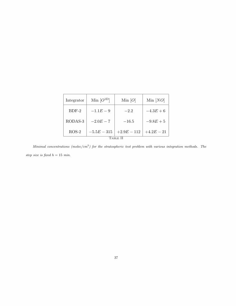
Integrator Min [O1D] Min [O] Min [NO]

BDF-2 −1.1E − 9 −2.2 −4.3E + 6

RODAS-3 −2.0E − 7 −16.5 −9.8E + 5

ROS-2 −5.5E − 315 +2.9E − 112 +4.2E − 21

Table II

Minimal concentrations (molec/cm3) for the stratospheric test problem with various integration methods. The

step size is fixed h = 15 min.

37

Integrator Standard Positive Overhead

BDF-2 506 Kflops 755 Kflops 50%

RODAS-3 652 Kflops 982 Kflops 50.6%

ROS-2 485 Kflops 502 Kflops 3.6%

Table III

The number of flops for integrating the small stratospheric test problem with various algorithms using both the

standard and the positive versions. The step size is fixed h = 15 min.

38

Integrator Clipping Projection Variable step

h = 15 min h = 30 min h = 15 min h = 30 min (rtol = 0.01)

ROS-2 543 Kflops 272 Kflops 566 Kflops 303 Kflops 3,798 Kflops

Table IV

The number of flops for integrating the small stratospheric test problem with ROS-2, fixed step size h = 15 min

for clipping and projection, and variable step size.

39