A periodically forced ﬂow displaying symmetry breaking via ...

Physica D 156 (2001) 81–97

A periodically forced flow displaying symmetry breaking via athree-tori gluing bifurcation and two-tori resonances

F. Marques a, J.M. Lopez b,∗, J. Shen c

a Departament de Fısica Aplicada, Universitat Politècnica de Catalunya, Jordi Girona Salgado s/n,Mòdul B4 Campus Nord, 08034 Barcelona, Spain

b Department of Mathematics, Arizona State University, Tempe, AZ 85287-1804, USAc Department of Mathematics, University of Central Florida, Orlando, FL 32816-1364, USA

Received 9 October 2000; received in revised form 26 February 2001; accepted 14 March 2001Communicated by S. Fauve

Abstract

The dynamics due to a periodic forcing (harmonic axial oscillations) in a Taylor–Couette apparatus of finite length isexamined numerically in an axisymmetric subspace. The forcing delays the onset of centrifugal instability and introducesa Z2 symmetry that involves both space and time. This paper examines the influence of this symmetry on the subsequentbifurcations and route to chaos in a one-dimensional path through parameter space as the centrifugal instability is enhanced.We have observed a well-known route to chaos via frequency locking and torus break-up on a two-tori branch once the Z2

symmetry has been broken. However, this branch is not connected in a simple manner to the Z2-invariant primary branch. Anintermediate branch of three-tori solutions, exhibiting heteroclinic and homoclinic bifurcations, provides the connection. Onthis three-tori branch, a new gluing bifurcation of three-tori is seen to play a central role in the symmetry breaking process.© 2001 Elsevier Science B.V. All rights reserved.

Keywords: Periodic forcing; Taylor–Couette flow; Symmetry breaking; Gluing bifurcation; Naimark–Sacker bifurcation

1. Introduction

The Taylor–Couette flow is canonical for thestudy of centrifugal instabilities and the study of lowco-dimension bifurcations with symmetry [8]. In theclassical setting, Taylor–Couette flow is studied inthe limit of infinite length cylinders and it is assumedthat the flow is periodic in the axial direction. Thisimposes a certain symmetry group on the system,SO(2) × O(2), where the SO(2) comes from theinvariance to rotations about the axis and the O(2)from the axial periodicity which allows invariance

∗ Corresponding author.E-mail address: [email protected] (J.M. Lopez).

to continuous translations in the axial direction andto reflection about a plane orthogonal to the axis. Inphysical settings with annular aspect ratios of lengthto gap of the order of 10 times the gap or less, thepresence of end walls has a profound influence onthe dynamics [3,4], principally due to the change insymmetry group from O(2) to Z2 [15]. The Z2 sym-metry comes from the invariance to reflection aboutthe mid-plane orthogonal to the axis.

In this study, we are interested in exploring the dy-namics due to a periodic forcing in a Taylor–Couettesetting with aspect ratio of order 10, where end-walleffects will be predominant. The particular forcing ofinterest here is that due to harmonic oscillations of theinner cylinder in the axial direction. Experiments [33]

0167-2789/01/$ – see front matter © 2001 Elsevier Science B.V. All rights reserved.PII: S0 1 6 7 -2 7 89 (01 )00261 -5

82 F. Marques et al. / Physica D 156 (2001) 81–97

have clearly demonstrated that this forcing is very ef-ficient in postponing the onset of centrifugal instabil-ity to significantly higher rotation rates of the innercylinder. This forcing changes the symmetry group ina subtle manner, although the symmetry group con-tinues to be SO(2)×Z2, the Z2 now mixes space andtime. The Z2 in the forced system is generated bythe combined reflection about the mid-plane togetherwith a half forcing period translation in time. As waspointed out some years ago [23], Z2 is the importantsymmetry in the Taylor–Couette problem. Our mainobjective is to study how this particular form of Z2

influences the nonlinear dynamics.To isolate the influence of the Z2 symmetry, we

study the flow in an SO(2)-invariant subspace. Exper-iments [33] and Floquet analysis [20,21] have shownthat the onset of centrifugal instability in the largeaspect ratio limit is axisymmetric over an extensiverange of parameter space, including the values con-sidered in this study; in addition, the bifurcationswe have found take place in a very small parame-ter region, close to the bifurcation point, making theassumption of axisymmetry highly plausible. Further-more, experiments in Taylor–Couette with the sameaspect ratio [6,31,32] show the presence of an axisym-metric very low frequency (VLF) mode, analogousto the three-tori we have found, although the flowis fully three-dimensional. Numerical simulations incylindrical flows driven by rotation [17] show that thedynamics is governed by axisymmetric secondary bi-furcations of the base flow, although the flows are fullythree-dimensional; in this case, the nonaxisymmetricmodes have less than 1% of the kinetic energy of theflow [5], and the agreement between experiments andaxisymmetric simulations is impressive [27]. All theseevidences provide further motivation for the restrictionto an axisymmetric subspace for the present study.

In this study, we hold constant the parameters gov-erning the geometry of the apparatus and the axialforcing, and consider a one-dimensional path throughparameter space, where the rotation of the inner cylin-der is progressively increased to see how the centrifu-gal instability manifests itself. Along the way, the Z2

symmetry is broken and a generic route to chaos viafrequency locking and torus break-up follows. The

manner in which Z2 is broken, however, is new in-volving heteroclinic and homoclinic bifurcations ofthree-tori (T3). In fact, the Z2-symmetry breaking thatis found corresponds to a gluing bifurcation of T3.This bifurcation was first reported in [16] and here,we provide a comprehensive analysis of how it plays acentral role in the nonlinear dynamics of this system.

In Section 2, we describe the governing equationsand symmetries of the system and the numerical tech-niques used. In Section 3, the primary branch whichundergoes a supercritical Naimark–Sacker bifurcationis analyzed and the physical mechanism responsiblefor the second frequency is elucidated. In Section 4,the T3 branch which undergoes the gluing bifurca-tion and symmetry breaking is examined. The routeto chaos on the secondary branch is presented in Sec-tion 5. Finally, in Section 6, an overview of how allthe various branches are interrelated is presented.

2. Governing equations

The system in question is the flow between twoco-axial cylinders of finite extent, the outer one beingstationary and the inner one rotating at constant an-gular velocity Ωi and oscillating in the axial directionwith velocityW sinΩf t . The top and bottom end-wallsare stationary. The geometry is shown schematicallyin Fig. 1. The radii of the cylinders are ri and ro (in-ner and outer, respectively), and their length is L; theannular gap between the cylinders is d = ro − ri.These parameters are combined to give the following

Fig. 1. Schematic representation of the flow configuration.

F. Marques et al. / Physica D 156 (2001) 81–97 83

nondimensional governing parameters: the radius ra-tio, e = ri/ro; the aspect ratio, Λ = L/d; the Cou-ette flow Reynolds number, Ri = driΩi/ν; the axialReynolds number, Ra = dW/ν; the nondimensionalfrequency, ωf = d2Ωf/ν, where ν is the kinematicviscosity of the fluid.

The length and time scales used are the gap, d, andthe diffusive time across the gap, d2/ν, respectively.With these scalings, the Navier–Stokes equations andthe incompressibility condition become

∂tv + (v · )v = −p + v, · v = 0. (1)

The boundary conditions are no-slip on all walls.This leads to discontinuous boundary conditions forthe axial and azimuthal components of velocity wherethe moving inner cylinder meets the stationary top andbottom end-walls. These discontinuities in a physicalexperiment correspond to a small, but finite gap (seefor example, Refs. [27,33]) and in Section 2.2, wedescribe how this is treated numerically.

The basic flow is time-periodic with period Tf =2π/ωf and synchronous with the forcing, and it isindependent of the azimuthal coordinate. The imposedperiodic forcing in this problem implies the existenceof a global Poincaré map, P, i.e. strobing with theforcing frequency ωf .

2.1. Symmetry considerations

The Navier–Stokes equations governing this prob-lem are invariant under rotations of angle α, Rα ,around the common axis of the cylinders, generatingthe symmetry group SO(2). Moreover, the equationsare invariant under an additional discrete symmetry,S, involving time and the axial coordinate; it is areflection about the mid-plane orthogonal to the axiswith a simultaneous time-translation of a half period.Using cylindrical coordinates, they read

(Rαv)(r, θ, z, t) = v(r, θ + α, z, t),

α ∈ R mod 2π, (2)

(Sv)(r, θ, z, t) = (u, v,−w)(r, θ,−z, t + 1

2Tf

)(3)

where v is the velocity field and (u, v,w) are the com-ponents in cylindrical coordinates. The symmetry S

satisfies S2 = I , and the symmetry group of our prob-lem is SO(2)×Z2. The SO(2) factor comes from Rα

and the Z2 factor is generated by S.The basic state, a limit cycle, is invariant under the

full symmetry group of the equations, SO(2) × Z2.It can lose stability when at least one Floquet multi-plier λ crosses the unit circle. In general, this may oc-cur through λ = +1 (synchronous bifurcation), λ =−1 (subharmonic bifurcation) or a pair of complexconjugate multipliers cross (Naimark–Sacker bifurca-tion). In a system without symmetries, the λ = +1case corresponds to the saddle-node bifurcation, theλ = −1 case corresponds to a period doubling andthe complex conjugate case is the Naimark–Sacker bi-furcation. However, when the Z2 symmetry group ispresent, it inhibits the period doubling (λ = −1) bi-furcation [29], the synchronous bifurcation becomes apitchfork and the Naimark–Sacker bifurcation resultsin a Z2-invariant T2 [14].

In this study, we solve the system in an axisym-metric subspace invariant to SO(2). Linear stabilityanalyses in the limit Λ → ∞, as well as experimentswith Λ = 150 have shown that over an extensiverange of parameter space, the primary bifurcation isto an axisymmetric state, periodic in the axial direc-tion and synchronous with the forcing, and only insmall windows of parameter space have nonaxisym-metric flows been observed [20,21,33]. Therefore, theonly nontrivial symmetry of the axisymmetric systemconsidered is S.

2.2. Numerical solution technique

The nonlinear axisymmetric Navier–Stokes equa-tions (1) are solved employing a highly efficient andaccurate spectral-projection method [19] in which thetime variable is discretized by using a second-orderprojection scheme [25,30] and the spatial variablesare discretized by using a spectral-Galerkin method[24,26].

The flow starts either from rest or as a continuationfrom a solution with different parameter values andsatisfies the following boundary conditions:

u = 0, v = Ri, w = Ra sinωf t at r = ri,

u = v = w = 0 at r = ro and z = ± 12Λ. (4)


This flow has discontinuous boundary conditions forthe azimuthal, v, and axial, w, components of ve-locity where the inner cylinder meets the stationaryend-walls. Since spectral methods are very sensitive tothe smoothness of the solutions, it is crucial to designa sensible treatment for the discontinuous boundaryconditions. This discontinuity is a mathematical ide-alization of the physical situation (a small finite gap).Therefore, it is appropriate to use a regularized bound-ary layer function to approximate the actual physicalsituation. In fact, the discontinuous boundary condi-tions at z = ± 1

2Λ

v = 0 for r ∈ (ri, ro] and v = Ri at r = ri,

and

w = 0 for r ∈ (ri, ro] and

w = Ra sinωf t at r = ri

can be approximated, respectively, by

vε(r) = Ri exp

(− r − ri

ε

), r ∈ [ri, ro], (5)

and

wε(r) = Ra sinωf t exp

(− r − ri

ε

), r ∈ [ri, ro]

(6)

to within any prescribed accuracy by choosing an ap-propriate ε. Such an approach has been proven suc-cessful in [19] for treating the discontinuous boundarycondition for the v component. Numerical modelingof the corner singularity for the Taylor problem hasbeen discussed previously in [10] using a different nu-merical method.

In this study, the axisymmetric Navier–Stokes equa-tions have been solved with the spectral scheme de-scribed in [18], using 80 axial and 64 radial modes,and a time-step δt = 1

200Tf . With 64 modes in the ra-dial direction, we were able to use ε = 0.005 in (5)and (6), which corresponds to the physical separationbetween the end-wall and side wall in typical exper-iments with d ∼ 1 cm. Note that further reducing ε

without increasing the radial resolution would intro-duce unwanted oscillations. We only consider varia-

tions in Ri, keeping all other parameters fixed (Λ =10, e = 0.905, Ra = 80, ωf = 30).

For axisymmetric flows in cylindrical geometries,it is typical to present the solutions in terms of thestreamfunction ψ , the azimuthal component of vortic-ity η and the axial component of the angular momen-tum γ = rv. The velocity vector can be written as

v = (u, v,w) =(

−1

r

∂ψ

∂z,γ

r,

1

r

∂ψ

∂r

),

and the vorticity vector as

× v =(

−1

r

∂γ

∂z, η,

1

r

∂γ

∂r

),

where

η = ∂u

∂z− ∂w

∂r= −1

r

(∂2ψ

∂z2+ ∂2ψ

∂r2− 1

r

∂ψ

∂r

). (7)

We solve the governing equations using velocity andpressure, and then the azimuthal vorticity η is foundby spectral differentiation of u and w, the stream func-tion ψ is found by solving the Helmholtz equation (7)and γ by spectral multiplication of rv. Note that in ameridional plane (r, z), contours of ψ are projectionsof the streamlines and contours of γ are projectionsof the vortex lines.

3. The primary branch

In this section, we describe the dynamics alongthe primary branch, the branch of solutions that issmoothly connected to the basic state at Ri = 0. Thisbasic state corresponds essentially to an annular Stokesflow, the annular analogue of the flow driven by thein-plane harmonic oscillation of a plate [28], but ismodified by: (i) the presence of end-walls and (ii) theouter cylinder. The presence of these walls enforcesa zero mass flux, so that on the up (down) stroke ofthe inner cylinder there is a return flow down (up) theouter cylinder. Most of the features of the basic stateare common to the limiting case Λ → ∞ [20], buthere the end-walls will be shown to play a significantrole in the subsequent dynamics of the flow as Ri isincreased.


Fig. 2. Contours depicting: (a) vortex lines and (b) streamlines at 10 equispaced phases over one complete forcing period T for the T1

solution on the primary branch for Ri = 280.0.

In the limiting case Λ → ∞, increase in Ri led tocentrifugal instability of the basic state, however, thepresence of end-walls separated by a finite distanceleads to a smooth transition. In the Λ → ∞ case, thebifurcation is a pitchfork of revolution and the bifur-cating solutions differ in phase (a spatial translationalong the axis). In fact, in most numerical settings, aplanar pitchfork is obtained because the phase is fixedexcept for a shift (a sign in the amplitude); a de-tailed discussion, both theoretical and experimental inthe Taylor–Couette problem can be found in [9]. Thepresence of end-walls generates a z-dependent flowclose to the end-walls that progressively fills the wholedomain when Ri is increased. At finite Ri, the flow onthe primary branch is characterized by the presenceof jets emanating from the inner cylinder boundarylayer that advect the vortex lines into the interior (seeFig. 2(a)) and associated with these jets, the stream-lines have a cellular structure reminiscent of Taylorvortices (see Fig. 2(b)). The jets are dragged up anddown by the motion of the inner cylinder, synchronouswith the forcing. This basic state is a limit cycle (T1)

and retains all the symmetries of the system.When Ri is increased beyond a critical value, a

Naimark–Sacker bifurcation [14] leads to flow on aT

2. The basic state, being a T1, is a point in the

Poincaré section whereas the T2 is a closed loop in P.Fig. 3(a) shows the Poincaré sections of the solutionsfor Ri = 280.1–280.8 in steps of 0.1. Ri = 280.1 isbefore the supercritical Naimark–Sacker bifurcation.The amplitudes of the loops corresponding to the T2

scales with√

Ri − Ric, where Ric is the critical Ri atthe bifurcation. In Fig. 3(b), these amplitudes and thecorresponding fit are shown, and allow an estimate ofRic = 280.188. The phase portraits are in the (Γ,U)

plane, where Γ and U are the γ and u evaluated ata convenient Gauss–Lobato point in the annulus (r =ri + 0.573, z = 0.969).

Although resonance horns (Arnold’s tongues) areoften associated with Naimark–Sacker bifurcations,over the range of Ri where the T2 bifurcating fromthe primary T1 branch is stable, we have not observedany intervals of frequency locking. On the T2, one fre-quency is fixed, determined by the forcing frequencyωf = 30, and the second frequency, ωs, varies with Riin the range 5.2–5.4. So, the bifurcated solutions arequasi-periodic and hence are not S-invariant. However,the T2 on which the solutions reside is S-invariant; wehave taken a bifurcated solution, applied the S sym-metry, and found that this transformed solution re-sides on the same T2. Naimark–Sacker bifurcations inODE systems with Z2 symmetry (not involving time)


Fig. 3. Poincare sections of the solutions on the primary branch depicting the T1 solution at Ri = 280.1 as a point and the successive T2

solutions for Ri = 280.2 + 0.1n with n ∈ [0, 6] as the cycles with amplitude increasing with Ri and (b) variation of the amplitudes in (a)with Ri.

always result in an Z2-invariant T2 [14]. Our Z2 gen-erated by S does involve time, yet we observe the samebehavior (an invariant T2 following the bifurcation) inour system.

To determine what the second frequency, ωs, cor-responds to, we have strobed the streamfunction atthe forcing frequency. Fig. 4 shows these strobed im-ages over 10 forcing periods. A T1 solution would beconstant in such a sequence. The T2 solution showsvariations that are concentrated in the top and bottomthirds of the cylinder while the central third does notchange. This suggests that ωs corresponds to an un-steady coupling between the end-wall vortices and thejets emanating from the boundary layer on the innercylinder. This is further discussed when comparing theflows on other branches in Section 5.

The T2 solution branch bifurcating from the pri-mary branch at Ri = 280.188 ceases to be stable be-yond Ri = 280.88. Attempts to continue the T2 solu-tion branch beyond Ri = 280.88 result in an evolutionto a three-torus (T3) solution. The theoretical studyof bifurcations of tori is difficult, some scenarios havebeen rigorously analyzed by generalizing Floquet the-ory in systems without symmetries [7]. To our knowl-edge, no such studies with Z2 symmetry have beenpublished.

Fig. 4. Streamlines of a solution on the primary branch withRi = 280.88, strobed over 10 periods at a fixed phase. Thirtycontour levels in the range [−75, 75] are used, solid (broken) linesindicate positive (negative) contour levels.

4. Three-tori branch

We have located a range (Ri ∈ [280.89, 281.26])where stable T3 solutions exist. Their characteristicsare elucidated with the aid of the global Poincaré mapP, time series and phase portraits in the (Γ,U) plane.


Fig. 5. (a) Power spectra of a T3 solution at Ri = 280.98, and (b) a zoom of the PSD in (a) near the origin.

The power spectral density (PSD) of the time se-ries of Γ , shown in Fig. 5(a), has a main peak at theforcing frequency, ωf = 30, a second frequency atωs ≈ 5.2, and their linear combinations since theseare incommensurate. This second frequency is veryclose to ωs of the T2 on the primary branch followingthe Naimark–Sacker bifurcation. The PSD also pos-sesses a VLF, ωVLF, which is three orders of magni-tude smaller than ωs. Fig. 5(b) is a zoom of (a) nearthe origin showing the peak at ωVLF and its harmon-ics. Due to the large spectral gaps between these threeincommensurate frequencies, we have been able to un-ambiguously characterize these solutions as T3.

Over the range of Ri where T3 solutions exist, ωs =5.2 ± 3%. In contrast, TVLF = 2π/ωVLF experiencesdramatic changes over this range, as shown in Fig. 6.This figure indicates that there are two Ri values whereTVLF becomes unbounded. For ease of discussion,we now represent T3 as limit cycles and T2 as fixedpoints. This analogy works since the two suppressedfrequencies, ωf and ωs are almost constant (in fact,ωf is constant), over the range of Ri of interest andthey do not play an essential role in the dynamics nearthe bifurcation points. Infinite-period bifurcations areusually associated with homoclinic or heteroclinic be-havior. The two most typical are the following: (i)a limit cycle collides with a hyperbolic fixed point

resulting in a homoclinic connection and then van-ishes; (ii) a saddle-node occurs on the limit cycle.These two scenarios are distinguished by the asymp-totic behavior of the period of the limit cycle as thebifurcation point is approached. In case (i), the pe-riod close to the bifurcation point would have theform [12]

TVLF ∼ λ−1hom ln

(1

|Ri − Ricrit|)

+ d, (8)

Fig. 6. Variation of TVLF = 2π/ωVLF with Ri. Symbols are com-puted values and solid lines are log fits.


while in case (ii) it has the form [14]

TVLF ∼ c√|Ri − Ricrit|+ d.

Our computed TVLF fits the logarithmic form verywell, whereas it does not adjust to the square rootform. The fitted logarithmic curves are the solid linesin Fig. 6 and the symbols are the computed periods.The fits are uniformly good over the whole range ofexistence of the T3, strongly suggesting that the ho-moclinic/heteroclinic behavior dominates the dynam-ics over the whole interval. The expression for thelogarithmic profile in the first section is given by

TVLF = λ−1het ln

1

|Ri−Rihet|+λ−1hom ln

1

|Ri − Rihom| + c.

In the entire second section, the logarithmic fit (8)was used. The logarithmic fits give the critical Ri forthe two infinite period bifurcations, Rihet = 280.88736and Rihom = 281.00884. The factors λhet and λhom arethe eigenvalues corresponding to the unstable directionof the hyperbolic fixed points [12], in our case theseare unstable T2. The values obtained are λhet = 2.43×10−3 and λhom = 5.81 × 10−3.

Fig. 7 shows the iterates of Γ under the map P

(for brevity, we shall refer to these as time series ofP (Γ )) and phase portraits in the (Γ,U) plane. Theseare given at three values of Ri, each close to the infiniteperiod bifurcation points depicted in Fig. 6. Fig. 7(a)corresponds to Ri = 280.89, the closest Ri value toRihet computed. The time series shows that the solu-tion trajectory spends a long time close to not one, buttwo unstable T2 with rapid excursions between them;this behavior is also apparent in the phase portrait.The two unstable T2 appear as two cycles and the tra-jectory in the phase portrait spends a long time nearthem. The rapid excursions appear as tubular mani-folds connecting them. As Ri → Ri+het, the T3 depictedin Fig. 7(a) becomes a heteroclinic three-manifold.This is illustrated schematically in Fig. 8. In this fig-ure, T2 are represented by fixed points and T3 by limitcycles, the bold (thin) cycles being (un)stable. TheT

3 is S-invariant, whereas the pair of unstable T2 towhich it connects heteroclinically at Rihet are not, butare related to each other via the S symmetry. The T3

collides with the two unstable T2 simultaneously dueto the S symmetry.

The infinite period bifurcation at Ri = Rihom ismore complicated as T3 exist on both sides of the bi-furcation. Approaching Rihom from below, the T3 isS-invariant and approaches an unstable T2 which isalso S-invariant. This is seen in the time series and thephase portrait (Fig. 7(b)) for Ri = 281.008, which isvery close to Rihom. The figure shows the presence oftwo distinct fast homoclinic excursions. At the bifur-cation point, Rihom, there exists two homoclinic loopsthat are related by the S symmetry. This is also illus-trated schematically in Fig. 8.

For Ri > Rihom, but close to the bifurcation, thebehavior is qualitatively different. Fig. 7(c) shows atRi = 281.009, the existence of a T3 close to an un-stable T2 with a single homoclinic excursion. We alsonote from Fig. 6 that for Ri > Rihom, the period TVLF

is significantly reduced from that when Ri < Rihom.Beyond Rihom, the double homoclinic loop splits intotwo T3 as shown in the schematic Fig. 8. The solu-tion in Fig. 7(c) corresponds to one of these T3, whichis no longer S-invariant. We have explicitly computedthe S-related partners for Ri > Rihom by applyingthe symmetry S to a trajectory on the first obtainedT

3, a trajectory on a different T3 results. These twodistinct T3 are S-symmetrically related. We have notbeen able to continue the T3 solution branches beyondRi = 281.26; the system evolves to another one corre-sponding to a T2 branch that is described in Section 5.

The range of Ri where T3 exist consists of twobranches, for Rihet < Ri < Rihom there is a singleS-invariant T3 and for Ri > Rihom a pair of non-symmetric, but symmetrically related, T3. The firstbranch starts in a heteroclinic bifurcation schemati-cally shown in Fig. 8 and is related to the secondbranch via a homoclinic bifurcation at Ri = Rihom.In this homoclinic bifurcation an S-invariant T3 splitsin two S-related T3. Analogous gluing bifurcations oflimit cycles in systems with Z2 symmetry have beenanalyzed in [13] and in [1] for systems with morecomplex (D4) symmetries. Here, we have a gluing bi-furcation of T3 in a real fluid system.

From Fig. 8, we see that three unstable T2 play akey role as organizing centers for the dynamics of the


Fig. 7. Time series of P(Γ ) (left) and phase portraits in the (Γ,U) plane (right) for Ri = 280.89 (a), 281.008 (b), 281.008 (b), 281.009 (c).


Fig. 8. Schematic representation of the bifurcation sequence for theT

3 solutions. In this schematic representation, T2 are representedas fixed points and T3 as cycles. The labels (a), (b) and (c)correspond to the three parts of Fig. 7.

stable T3. The unstable T2 in the center of Fig. 8 isS-invariant since it is central to the gluing bifurcation.Further, ωs is continuous along the primary branch andthe T3 branches, with the connection between thesebranches occurring at the homoclinic point Rihom.

We are able to explore the flow characteristics as-sociated with the S-invariant unstable T2 at points inparameter space where the stable T3 is almost homo-clinic to it, i.e. Ri ≈ Rihom. From Fig. 7(b), we seethat for approximately 3 × 105 iterates of P, the T3

remains very close to the unstable T2. In Fig. 9, weshow streamlines at 10 consecutive iterates of P, start-ing after the first 105 iterates in Fig. 9. Note that sinceωs ≈ 5.28, this sequence almost repeats itself everyωf/ωs ≈ 5.7 iterates of P for the subsequent 2 × 105

iterates of P. Fig. 9 displays the same behavior as

Fig. 9. Streamlines of a solution on the primary branch withRi = 281.008, while it is close to the unstable symmetric T2 atindicated multiples of the forcing period; contours levels as inFig. 4.

that in Fig. 4 which corresponds to the stable T2 onthe primary branch. This suggests that the unstable T2

and the stable T2 are on the same S-invariant solutionbranch (the primary branch).

For Ri ≈ Rihet, since the T3 passes close to twounstable T2 and remains close to them for long time(about 5 × 105 iterates of P), we are also able to ex-plore the flow characteristics associated with these T2.Fig. 10 shows the streamlines at 10 consecutive iter-ates of P; part (a) corresponds to times when the T3

is close to one of the unstable T2 and (b) to the other.The behavior is very similar to that in Fig. 9, show-ing the modulation due to ωs as oscillations near bothend-walls, the difference between each of the threecases is in the phase difference between the oscilla-tions near the top and bottom end-walls.

We have not been able to continue the T3 beyondRi > 281.26; the system evolves to another far offbranch that is described in the next section.

5. A route to chaos through resonance horns

The branch to be described here is robust in thesense that time evolution from an initial state of restevolves to this branch, even for Ri values for which


Fig. 10. Streamlines of a solution on the T3 branch for Ri = 280.89 while it is close to the: (a) unstable nonsymmetric T2 and (b) itssymmetric counter part, at indicated multiples of the forcing period; contours level as in Fig. 4.

the primary and the T3 branches coexist and are sta-ble. We have been able to continue this branch, whichwe shall denote as the secondary branch, down toRi = 280.46. For Ri < 280.46, the attempts to con-tinue this branch led to evolutions onto the primary T2

branch.

Fig. 11. Streamlines, at Ri = 280.9, strobed at a fixed phase of the forcing at indicated multiples of the forcing period for a solution on:(a) the secondary branch; (b) its S-related solution branch, contours level as in Fig. 4.

The main distinction between this secondary T2

branch and the primary T2 branch described in Sec-tion 3 is that the T2 here is not S-invariant. This isreadily determined by taking a solution on this branch,applying the S-symmetry and observing that the resul-tant solution trajectory resides on a different T2. We


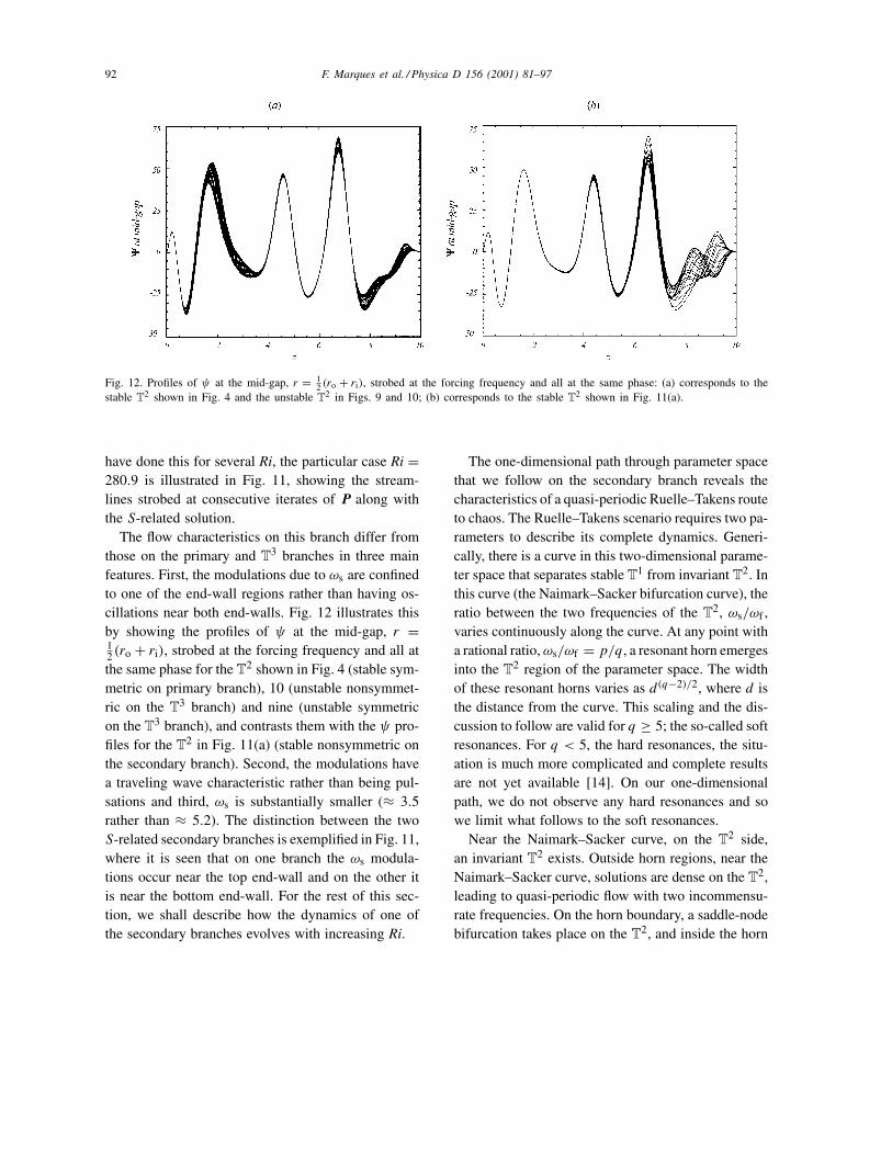
Fig. 12. Profiles of ψ at the mid-gap, r = 12 (ro + ri), strobed at the forcing frequency and all at the same phase: (a) corresponds to the

stable T2 shown in Fig. 4 and the unstable T2 in Figs. 9 and 10; (b) corresponds to the stable T2 shown in Fig. 11(a).

have done this for several Ri, the particular case Ri =280.9 is illustrated in Fig. 11, showing the stream-lines strobed at consecutive iterates of P along withthe S-related solution.

The flow characteristics on this branch differ fromthose on the primary and T3 branches in three mainfeatures. First, the modulations due to ωs are confinedto one of the end-wall regions rather than having os-cillations near both end-walls. Fig. 12 illustrates thisby showing the profiles of ψ at the mid-gap, r =12 (ro + ri), strobed at the forcing frequency and all atthe same phase for the T2 shown in Fig. 4 (stable sym-metric on primary branch), 10 (unstable nonsymmet-ric on the T3 branch) and nine (unstable symmetricon the T3 branch), and contrasts them with the ψ pro-files for the T2 in Fig. 11(a) (stable nonsymmetric onthe secondary branch). Second, the modulations havea traveling wave characteristic rather than being pul-sations and third, ωs is substantially smaller (≈ 3.5rather than ≈ 5.2). The distinction between the twoS-related secondary branches is exemplified in Fig. 11,where it is seen that on one branch the ωs modula-tions occur near the top end-wall and on the other itis near the bottom end-wall. For the rest of this sec-tion, we shall describe how the dynamics of one ofthe secondary branches evolves with increasing Ri.

The one-dimensional path through parameter spacethat we follow on the secondary branch reveals thecharacteristics of a quasi-periodic Ruelle–Takens routeto chaos. The Ruelle–Takens scenario requires two pa-rameters to describe its complete dynamics. Generi-cally, there is a curve in this two-dimensional parame-ter space that separates stable T1 from invariant T2. Inthis curve (the Naimark–Sacker bifurcation curve), theratio between the two frequencies of the T2, ωs/ωf ,varies continuously along the curve. At any point witha rational ratio,ωs/ωf = p/q, a resonant horn emergesinto the T2 region of the parameter space. The widthof these resonant horns varies as d(q−2)/2, where d isthe distance from the curve. This scaling and the dis-cussion to follow are valid for q ≥ 5; the so-called softresonances. For q < 5, the hard resonances, the situ-ation is much more complicated and complete resultsare not yet available [14]. On our one-dimensionalpath, we do not observe any hard resonances and sowe limit what follows to the soft resonances.

Near the Naimark–Sacker curve, on the T2 side,an invariant T2 exists. Outside horn regions, near theNaimark–Sacker curve, solutions are dense on the T2,leading to quasi-periodic flow with two incommensu-rate frequencies. On the horn boundary, a saddle-nodebifurcation takes place on the T2, and inside the horn


Fig. 13. Phase portraits for Ra = 80, ωf = 30, e = 0.905,Λ = 10 and Ri = 280.48 (a), 280.5 (b), 282 (c). For the locked cases, the orderin which the trajectory passes through the Poincare map is indicated.

a stable/unstable pair of limit cycle solutions exist onthe T2. In the generic two parameter scenario, at largedistance from the curve, the T2 may be destroyed.The Afraimovich–Shilnikov theorem [2] asserts threedistinct scenarios: (i) breakdown due to some typi-cal bifurcation of limit cycles, e.g. period doubling orsubsequent Naimark–Sacker bifurcations; (ii) abrupttransition to chaos via the appearance of a homoclinictrajectory; (iii) breakdown due to the loss of smooth-ness, i.e. wrinkling of the T2. On our one-dimensionalpath, we have observed scenarios (i) and (iii).

The phase portrait shown in Fig. 13(a) correspond-ing to Ri = 280.48, is that of an invariant circle. Thesecond frequency, ωs ≈ 3.8, is incommensurate withωf = 30. We have only been able to continue thisbranch down to Ri = 280.46, where ωs = 3.896. In-creasing Ri, our one-dimensional path passes through

Fig. 14. (a) Phase portrait for Ra = 80, ωf = 30, e = 0.905,Λ = 10 and Ri = 282.1; (b) a zoom of the boxed region in (a).

various resonance horns. The first, a 1:8 locking, is en-countered at Ri = 280.49 and extends to Ri = 280.7.The phase portrait in Fig. 13(b) shows this 1:8 lock-ing at Ri = 280.50, where we have labeled the orderin which the solution trajectory crosses the Poincarésection. Following an interval of quasi-periodicity atRi = 281.4, the 1:9 horn is encountered (at Ri =281.0, ghosting behavior near the 2:17 horn has beendetected). The 1:9 horn extends to Ri = 282 andFig. 13(c) shows the phase portrait at this Ri.

On leaving the 1:9 horn, the T2 displays evidence ofhaving lost smoothness. Fig. 14 shows the phase por-trait at Ri = 282.1 together with a zoom of the boxedregion. The solution at this Ri is actually a limit cycledue to a 3:28 locking; as the resonance horn is verynarrow, the transient approach to the limit cycle is veryslow. The transient trajectory allows us to visualize the


Fig. 15. Phase portraits for Ra = 80, ωf = 30, e = 0.905,Λ = 10 and Ri = 282.4 (a), and 282.5 (b). The order in which the trajectorypasses through the Poincare map is indicated.

underlying T2. It is clear that the T2 has lost smooth-ness, displaying the characteristic wrinkling observedin [11].

The 2:19 horn is entered on increasing Ri to 282.3.A phase portrait at Ri = 282.4 is shown in Fig. 15(a).The sequence of horns visited so far is as expectedfrom their Farey tree structure; we began with 1:8, then1:9, with a ghost of the 2:17 in between, then the 2:19,which is the widest horn between the 1:9 and 1:10. Wealso observed the wrinkling at the 3:28 between the1:9 and 2:19. Now, inside the 2:19, at Ri = 282.5 the2:19 limit cycle undergoes a period doubling to 4:38.In the range 282.5 ≤ Ri ≤ 282.7, we have observedthe 4:38 limit cycle. Fig. 15(b) shows the phase portraitat Ri = 282.5. This type of period doubling is one ofthe standard scenarios by which the T2 is destroyedaccording to the Afraimovich–Shilnikov theorem.

Fig. 17. Phase portraits for Ra = 80, ωf = 30, e = 0.905,Λ = 10. (a) Ri = 283.1, (b) a zoom of the boxed region in (a) and (c) Ri = 285.

Fig. 16. Schematic representation of the one-dimensional pathalong the secondary branch.

Along our one-dimensional path, the period doubledregion is exited and we re-enter the 2:19 region ofthe horn. A schematic representation of our path isshown in Fig. 16. On further increasing Ri, the 2:19horn is exited and from this point on, the T2 becomesincreasingly less smooth and eventually the flow is


chaotic. At Ri = 283.1, the wrinkling is illustrated inFig. 17(a) together with a zoom in (b) and the phaseportrait of a chaotic state at Ri = 285 is given inFig. 17(c).

6. Summary and conclusions

We have studied a one-dimensional route in param-eter space of a periodically forced flow with symmetry.As this parameter, Ri, is increased, the system under-goes a sequence of local and global bifurcations andbecomes chaotic. The route to chaos obtained involvesa new and convoluted symmetry breaking, involvingheteroclinic, homoclinic and gluing bifurcations ofT3.

An overall description of our one-dimensionalpath is schematically presented in Fig. 18. The solidcurves correspond to stable T1,T2 and T3 solutionbranches which were encountered. The dashed curvesconnecting them are conjectured based on the prop-erties of the stable solutions. The primary branch,consisting of S-invariant T1, undergoes a supercrit-ical Naimark–Sacker bifurcation to an S-invariantT

2. This is the generic scenario of a Z2-symmetricNaimark–Sacker [14]. The resulting T2 is S-invariant,but obviously the solutions (trajectories) on it are notS-invariant by virtue that the two frequencies on theT

2 are incommensurate. This T2 loses stability, butremains S-invariant as Ri is increased, and solutiontrajectories evolve to a T3.

Continuing the T3 branch to lower Ri, the branchceases to exist at a heteroclinic bifurcation as it col-

Fig. 18. Bifurcation diagram showing the primary, secondary andT

3 branches; the dashed lines are the unstable branches.

lides with two S-symmetrically related unstable T2;the T3 is S-invariant. Increasing Ri, the T3 becomeshomoclinic to an S-invariant unstable T2, which weconjecture is the unstable T2 from the primary branch.The conjecture is based on the close similarities ofthe corresponding oscillatory flows on the stable T2

and the unstable T2 to which the T3 becomes homo-clinic to. The secondary frequency, ωs, is continuousbetween the two T2, further supporting this conjec-ture. At the homoclinic point, the T3 suffers a sym-metry breaking gluing bifurcation. This is the onlysymmetry breaking bifurcation we have observed inthis system. The importance of the Z2 symmetry inthe Taylor–Couette problem and its association withcomplex dynamics (e.g. homoclinic and Shilnikov bi-furcations) was pointed out by [23], and was also re-viewed in [22].

Increasing Ri beyond a critical value, the T3 branchcannot be continued further and the flow evolves ontoa T2 that is not S-invariant. In fact, there are twosuch T2 branches, symmetrically related, along whicha standard (i.e. not influenced by symmetries) route tochaos via quasi-periodicity and locking in resonancehorns and torus break-up is observed.

The three T2 to which the T3 are either hetero-clinically or homoclinically asymptotic to the orga-nizing centers of the dynamics of the T3. In fact, theT

3 flows are essentially slow drifts, with VLF, be-tween the unstable T2. Similar VLF states have alsobeen observed experimentally [6,31,32] in an unforcedTaylor–Couette flow with aspect ratio of order 10, as isthe aspect ratio in our computations. Since their systemwas unforced, the VLF states manifested themselvesas T2. Furthermore, those observed VLF states arereported to be axisymmetric modes of oscillation be-tween the end-walls, even though the underlying flowis nonaxisymmetric [32]. We can reasonably expectthat our axisymmetric T3 solutions, even if they areunstable to nonaxisymmetric disturbances continue toplay an important role in the flow dynamics.

How are the various observed stable and unstableT

2 connected? As Ri decreases along the secondarybranch, ωs increases from 3.2 to 3.9, getting close toωs values on the primary T2 and the T3 branches. Thisleads us to conjecture that the unstable T2 heteroclinic


to the T3 and the stable secondary T2 branch mergeat a saddle-node bifurcation of T2 and cease to ex-ist at lower Ri. This is the lowest co-dimension bifur-cation consistent with the observed characteristics ofthe respective T2. All possible bifurcations of T2 is asubject that has not yet been exhaustively studied, but[7] describe the most likely scenarios associated witha real eigenvalue crossing the unit circle through ±1or the crossing of a pair of complex conjugate eigen-values. Both the −1 and the complex conjugate cross-ing would introduce a new frequency, which is not thecase in our system; the +1 crossing, since there is nosymmetry involved, corresponds to a saddle-node.

We also conjecture that on increasing Ri, the unsta-ble T2 associated with the T3 branch merge in a pitch-fork bifurcation of T2. We have been able to observethe flows on (near) these three T2 and they are all verysimilar (see Figs. 9 and 10), so it is reasonable that atlarge enough Ri, they merge. The simplest bifurcationconsistent with one symmetric and two symmetricallyrelated T2 is the pitchfork.

To further clarify these conjectured connections be-tween the stable and unstable T2, two tools are re-quired: (i) the computation and continuation with pa-rameter variation of unstable T2; (ii) a generalizedFloquet analysis for T2.

Acknowledgements

This work was partially supported by DGICYTgrant PB97-0685 and Generalitat de Catalunyagrant 1999BEAI400103 (Spain), and NSF grantsDMS-9706951, INT-9732637 and CTS-9908599(USA).

References

[1] D. Ambruster, B. Nicolaenko, N. Smaoui, P. Chossat,Symmetries and dynamics for 2D Navier–Stokes flow, PhysicaD 95 (1996) 81–93.

[2] V.S. Anishchenko, M.A. Safonova, L.O. Chua, Confirmationof the Afraimovich–Shilnikov torus-breakdown theorem via atorus circuit, IEEE Trans. Circuits Syst. I 40 (1993) 792–800.

[3] T.B. Benjamin, Bifurcation phenomena in steady flows of aviscous fluid, Proc. R. Soc. Lond. A 359 (1978) 1–26.

[4] T.B. Benjamin, T. Mullin, Anomalous modes in the Taylorexperiment, Proc. R. Soc. Lond. A 377 (1981) 221–249.

[5] H.M. Blackburn, J.M. Lopez, Symmetry breaking of the flowin a cylinder driven by a rotating endwall, Phys. Fluids 12(2000) 2698–2701.

[6] F.H. Busse, G. Pfister, D. Schwabe, Formation of dynamicalstructures in axisymmetric fluid systems, in: Evolution ofSpontaneous Structures in Dissipative Continuous Systems,Lecture Notes in Physics, Vol. m55, Springer, Berlin, 1998,pp. 86–126.

[7] A. Chenciner, G. Iooss, Bifurcation of invariant torus, Arch.Rat. Mech. Anal. 69 (1979) 109–198.

[8] P. Chossat, G. Iooss, The Couette–Taylor Problem, Springer,Berlin, 1994.

[9] K.A. Cliffe, J.J. Kobine, T. Mullin, The role of anomalousmodes in Taylor–Couette flow, Phil. Trans. R. Soc. Lond. A439 (1992) 341–357.

[10] K.A. Cliffe, T. Mullin, A numerical and experimental studyof anomalous modes in the Taylor experiment, J. Fluid Mech.153 (1985) 243–258.

[11] J.H. Curry, J.A. Yorke, A transition from Hopf bifurcation tochaos: computer experiments with maps in R2, in: J.C. Martin,N.G. Markley, W. Perrizo (Eds.), The Structure of Attractorsin Dynamical Systems, Springer Notes in Mathematics, Vol.668, Springer, Berlin, 1978, pp. 48–66.

[12] P. Gaspard, Measurement of the instability rate of afar-from-equilibrium steady state at an infinite periodbifurcation, J. Phys. Chem. 94 (1) (1990) 1–3.

[13] P. Glendinning, Bifurcations near homoclinic orbits withsymmetry, Phys. Lett. A 103 (1984) 163–166.

[14] Y.A. Kuznetsov, Elements of Applied Bifurcation Theory, 2ndEdition, Springer, Berlin, 1998.

[15] A.S. Landsberg, E. Knobloch, Oscillatory bifurcation withbroken translation symmetry, Phys. Rev. E 53 (1996) 3579–3600.

[16] J.M. Lopez, F. Marques, Dynamics of 3-tori in a periodicallyforced Navier–Stokes flow, Phys. Rev. Lett. 85 (2000) 972–975.

[17] J.M. Lopez, F. Marques, J. Sanchez, Oscillatory modes in anenclosed swirling flow, J. Fluid Mech. (2001), in press.

[18] J.M. Lopez, F. Marques, J. Shen, Endwall effects in aperiodically forced centrifugally unstable flow, Fluid Dyn.Res. 27 (2000) 91–108.

[19] J.M. Lopez, J. Shen, An efficient spectral-projection methodfor the Navier–Stokes equations in cylindrical geometries. I.Axisymmetric cases, J. Comput. Phys. 139 (1998) 308–326.

[20] F. Marques, J.M. Lopez, Taylor–Couette flow with axialoscillations of the inner cylinder: Floquet analysis of the basicflow, J. Fluid Mech. 348 (1997) 153–175.

[21] F. Marques, J.M. Lopez, Spatial and temporal resonances ina periodically forced extended system, Physica D 136 (2000)340–352.

[22] T. Mullin, Disordered fluid motion in a small closed system,Physica D 62 (1993) 192–201.

[23] T. Mullin, K.A. Cliffe, Symmetry breaking and the onset oftime dependence in fluid mechanical systems, in: S. Sarkar(Ed.), Nonlinear Phenomena and Chaos, Adam Hilger, Bristol,1986, pp. 96–112.


[24] J. Shen, Efficient spectral-Galerkin method. I. Direct solversfor second-and fourth-order equations by using Legendrepolynomials, SIAM J. Sci. Comput. 15 (1994) 1489–1505.

[25] J. Shen, Efficient Chebyshev–Legendre Galerkin methods forelliptic problems, in: A.V. Ilin, R. Scott (Eds.), Proceedingsof ICOSAHOM’95, Houston J. Math. (1996) 233–240.

[26] J. Shen, Efficient spectral-Galerkin methods. III. Polar andcylindrical geometries, SIAM J. Sci. Comput. 18 (1997)1583–1604.

[27] J.L. Stevens, J.M. Lopez, B.J. Cantwell, Oscillatory flowstates in an enclosed cylinder with a rotating end-wall, J.Fluid Mech. 389 (1999) 101–118.

[28] G.G. Stokes, On the effect of the internal friction of fluids onthe motion of pendulums, Trans. Camb. Phil. Soc. 9 (1851) 8.

[29] J.W. Swift, K. Wiesenfeld, Suppression of period doublingin symmetric systems, Phys. Rev. Lett. 52 (1984) 705–708.

[30] J. van Kan, A second-order accurate pressure correctionscheme for viscous incompressible flow, SIAM J. Sci. Stat.Comput. 7 (1986) 870–891.

[31] J. von Stamm, T. Buzug, G. Pfister, Frequency locking inaxisymmetric Taylor–Couette flow, Phys. Lett. A 194 (1994)173–178.

[32] J. von Stamm, U. Gerdts, T. Buzug, G. Pfister, Symmetrybreaking and period doubling on a torus in the VLF regime inTaylor–Couette flow, Phys. Rev. E 54 (5) (1996) 4938–4957.

[33] A.Y. Weisberg, I.G. Kevrekidis, A.J. Smits, Delayingtransition in Taylor–Couette flow with axial motion of theinner cylinder, J. Fluid Mech. 348 (1997) 141–151.

A periodically forced ﬂow displaying symmetry breaking via ...

Documents

Transcript of A periodically forced ﬂow displaying symmetry breaking via ...