A Perfectly Matched Layer for the Helmholtz Equation in a ...turkel/PSmanuscripts/ido_pml.pdf ·...

default A Perfectly Matched Layer for the

Helmholtz Equation in a Semi-infinite Strip

I. Singer a E. Turkel a,∗

aDepartment of MathematicsTel Aviv University

Tel Aviv, Israel

history

Abstract

The Perfectly Matched Layer (PML) has become a widespread technique for pre-venting reflections from far field boundaries for wave propagation problems in boththe time dependent and frequency domains. We develop a discretization to solvethe Helmholtz equation in an infinite two dimensional strip. We solve the interiorequation using high-order finite differences schemes. The combined Helmholtz-PMLproblem is then analyzed for the parameters that give the best performance. Weshow that the use of local high-order methods in the physical domain coupled witha specific second order approximation in the PML yields global high-order accuracyin the physical domain. We discuss the impact of the parameters on the effectivenessof the PML. Numerical results are presented to support the analysis.

keywords. Key words: Helmholtz, PML, finite difference1991 MSC: 65N06

1 Introduction

The Helmholtz equation

∆u + k2u = 0, (1)

describes a wide variety of wave propagation phenomena including electromag-netic waves and acoustics. To solve this equation in an unbounded domain ona computer, one approach is to truncate the unbounded domain and intro-duce a boundary condition on the artificial outer surface. For many years the

∗ Corresponding Author.Email address: [email protected] (E. Turkel).

Preprint submitted to Journal of Computational Physics

standard boundary condition was a local absorbing condition that was a gen-eralization of the Sommerfeld radiation condition e.g. [4], but in recent years anumber of models based on the PML (Perfectly Matched Layers) scheme havebecome popular. These layers minimize the reflections caused by the artificialboundary.

Berenger [5],[6] was the first to introduce a PML for the time dependentMaxwell equations. Abarbanel and Gottlieb [1] proved that this approach isnot well posed and since then several other approaches generalizing the ideasof Berenger have been suggested. A survey of PML layers is to be found in[8]. Turkel and Yefet [16] showed that several of these approaches are linearlyequivalent. The solvability and the uniqueness of the PML equation for theHelmholtz equation was analyzed by Turkel and Tsynkov in [13]. In theirpaper, the decaying function inside the PML was assumed to be, for conve-nience of the analysis, a constant. This choice is not suitable for numericalcomputations.

We are interested in obtaining high accuracy for the approximation to theHelmholtz equation. In particular we shall consider both fourth and sixthorder accurate approximations in the physical domain. Hence, we shall use aPML in the far field to minimize reflections and so hopefully maintain the highaccuracy of the interior scheme. We extend [13] and search for a practical set ofparameters in the PML layer based on an analysis of the error in the combinedproblem. We also analyze the solvability and accuracy of the PML schemesfor this problem. The physical PML-Helmholtz scheme, which we develop, isthen solved by using high order finite differences schemes specially designedfor the Helmholtz equation. For a constant value of k in (1) we developed asixth order accurate scheme (and a fourth order accurate scheme for a variablek [9]). We analyze the effect of the use of these schemes on the solution and wefind conditions required for convergence. We also verify the assumption madein [13] that the overall accuracy of the Helmholtz-PML scheme depends onlyof the order of accuracy inside the physical domain where we solve the pureHelmholtz equation. We support our analysis with numerical results.

In order to invert the linear system one frequently uses iterative solvers. In thelast section we construct a preconditioner specially tailored for the combinedproblem. This preconditioner can be used with any Krylov space method.

In designing and analyzing the PML-Helmholtz equation, we use the two di-mensional notation of acoustics [13] and [16] for a waveguide. In two spacedimensions this is equivalent to the TE version of Maxwell’s equations. De-noting u as the pressure, we get (see for example [16])

∂

∂x

(Sy

Sx

ux

)+

∂

∂y

(Sx

Sy

uy

)+ k2SxSyu = 0. (2)

2

where

Sx = 1 +σx

ik, Sy = 1 +

σy

ikand σx and σy are functions of only x, y respectively. When σx = σy = 0this reduces to the Helmholtz equation (1). In the rest of the paper we onlyconsider the strip so σy = 0 and hence Sy = 1.

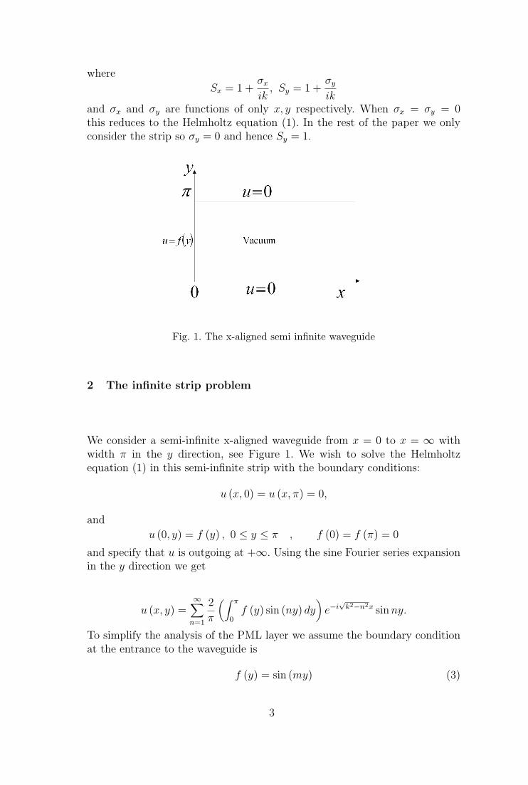
Fig. 1. The x-aligned semi infinite waveguide

2 The infinite strip problem

We consider a semi-infinite x-aligned waveguide from x = 0 to x = ∞ withwidth π in the y direction, see Figure 1. We wish to solve the Helmholtzequation (1) in this semi-infinite strip with the boundary conditions:

u (x, 0) = u (x, π) = 0,

and

u (0, y) = f (y) , 0 ≤ y ≤ π , f (0) = f (π) = 0

and specify that u is outgoing at +∞. Using the sine Fourier series expansionin the y direction we get

u (x, y) =∞∑

n=1

2

π

(∫ π

0f (y) sin (ny) dy

)e−i

√k2−n2x sin ny.

To simplify the analysis of the PML layer we assume the boundary conditionat the entrance to the waveguide is

f (y) = sin (my) (3)

3

where m is an integer. Then we get the exact solution which we label uexact

uexact (x, y) = e−i√

k2−m2x sin my. (4)

In the case m > k (evanescent wave) we get

uexact (x, y) = e−√

m2−k2x sin my

3 Constructing the PML

Since we cannot solve the semi-infinite problem on a computer we insteadsolve in a bounded domain: [0, L1] × [0, π], and construct a PML. We firstanalyze an infinite PML and then a PML with width L2 − L1, see Figure 2.

Fig. 2. The PML layer in the strip

In the interior of the strip (vacuum) we solve the Helmholtz equation and inthe PML we solve equation (2). In this case we choose σy = 0 in the PML andso Sy =1 and (2) becomes

∂

∂x

(1

Sx

ux

)+

∂

∂y(Sxuy) + k2Sxu = 0, Sx = Sx(x). (5)

Using the Fourier series expansion in y we get

d

dx

(1

Sx

du (x, n)

dx

)+ Sx

(k2 − n2

)u (x, n) = 0. (6)

We set

Sx (x) =

1 0 ≤ x ≤ L1

1 + σx

ikx > L1

(7)

4

We generalize this by considering Sx (x) = A + σx

B+ik. Our computational

results show that the error deteriorates when A differs appreciably from 1.Choosing B non-zero only slightly improves the accuracy. Equation (6) repre-sents u in the entire space (vacuum + PML). Substituting

t =∫ x

0Sx (r) dr

and labelingYn (t) = u (x, n)

we get for Yn (t) an equation with constant coefficients

d2

dt2Yn (t) +

(k2 − n2

)Yn (t) = 0.

The solution is

u (x, n) = c+ei√

k2−n2∫ x

0Sx(r)dr + c−e−i

√k2−n2

∫ x

0Sx(r)dr (8)

where c+ and c− are arbitrary constants. The solution for (6) in an infinitePML is found when we add the condition that only the right-traveling wavesare present in addition to the condition in x = 0.

Using (3) we get the solution for (5) which we label uI−pml (Infinite-PML):

uI−pml (x, y) =

e−i

√k2−m2

∫ x

0Sx(r)dr sin my if m < k

e−√

m2−k2∫ x

0Sx(r)dr sin my if m > k

. (9)

Comparing (4) with (9) we get for 0 ≤ x ≤ L1 :

uI−pml (x, y) = uexact (x, y)

which shows that the PML is perfectly non-reflecting.

When solving the problem on a computer we need to truncate the semi-infinitedomain at L2. We choose the boundary condition as u = 0 at x = L2. Choosingother types of boundary conditions at x = L2 does not significantly changethe solution. Hence, instead of c+ = 0 in (8) we need to solve (6) with theboundary condition u (L2, n) = 0. For our choice of f (y) = sin (my), withn 6= m, u (x, n) = 0 and boundary conditions

u (0, m) = 1 u (L2, m) = 0.

we get

u (x, m) = c+ei√

k2−m2∫ x

0Sx(r)dr + c−e−i

√k2−m2

∫ x

0Sx(r)dr

5

Solving for c+ and c−

c+ =−1

η − 1c− =

η

η − 1

where

η = e2i√

k2−m2∫ L20

Sx(r)dr. (10)

Uniqueness is not guaranteed when η = 1. Otherwise

2i√

k2 −m2

∫ L2

0Sx (r) dr = 2i

√k2 −m2

(L2 +

1

ik

∫ L2

L1

σx (r) dr

)

since σx (x) > 0 for x ∈ (L1, L2], then for k 6= m it follows that Re(2i√

k2 −m2∫ L20 Sx (r) dr

)6=

0 and η 6= 1 and uniqueness follows. Henceforth, we assume that k 6= m .

Labeling this unique solution uF−pml (Finite PML) we find

uF−pml =

(−1

η − 1ei√

k2−m2∫ x

0Sx(r)dr +

η

η − 1e−i

√k2−m2

∫ x

0Sx(r)dr

)sin my (11)

and for the case m < k (travelling)

error(x, y) = uI−pml − uF−pml

=1

η − 1

(ei√

k2−m2∫ x

0Sx(r)dr − e−i

√k2−m2

∫ x

0Sx(r)dr

)sin (my)

=2i

η − 1sin

(√k2 −m2

∫ x

0Sx (r) dr

)· sin (my) .

We are interested in the solution in the interior and so we examine the errorwhen 0 ≤ x ≤ L1

‖error(x, y)‖∞ (12)

= max0≤x≤L1, 0≤y≤π

∣∣∣∣∣ 2i

η − 1sin

(√k2 −m2x

)· sin (my)

∣∣∣∣∣=

∣∣∣∣∣ 2

η − 1

∣∣∣∣∣ .Our goal is to minimize the error and so we choose a suitable function σx (x)

that will minimize the value of∣∣∣ 2η−1

∣∣∣. We wish η in (10) to satisfy |η| >> 1.

For the case m > k (evanescent) we get

6

error(x, y) = uI−pml − uF−pml

=η

η − 1

(e−√

m2−k2∫ x

0Sx(r)dr − e

√m2−k2

∫ x

0Sx(r)dr

)sin (my)

=− 2η

η − 1sinh

(√m2 − k2

∫ x

0Sx (r) dr

)· sin (my)

and in the interior

‖error(x, y)‖∞ '∣∣∣∣∣ η

η − 1e√

m2−k2L1

∣∣∣∣∣ . (13)

In this case we wish in (10) that |η| << 1.

4 Minimizing the error

The function σx : [L1, L2] → R is chosen so that it has the following properties:

σx (x) > 0 for x ∈ (L1, L2]

σx (L1) = 0

σx (x) is smooth in [L1, L2] .

A suitable choice for this function is

σx (x) = σ(

x− L1

L2 − L1

)p

(14)

where σ is a positive constant and p ≥ 1. When evanescent waves are presentit may be more advantageous to use an exponential fit for σx. In this studywe shall only consider the polynomial fit. Integrating we get

∫ x

L1

σx (r) dr =σ (L2 − L1)

p + 1

(x− L1

L2 − L1

)p+1

and

uF−pml = sin my · (15)

−1η−1

ei√

k2−m2x + ηη−1

e−i√

k2−m2x 0 < x ≤ L1

−1η−1

ei√

k2−m2L1+√

1−εσ(L2−L1)

p+1

(x−L1

L2−L1

)p+1

+

ηη−1

e−i√

k2−m2L1−√

1−εσ(L2−L1)

p+1

(x−L1

L2−L1

)p+1 L1 < x ≤ L2

7

where ε =(

mk

)2and

η = e2i√

k2−m2∫ L20

Sx(r)dr = e2i√

k2−m2L2+2σ√

1−ε(L2−L1)

p+1 . (16)

For m < k we get

|η| = e2σ√

1−ε(L2−L1)

p+1 >> 1

and for m > k|η| = e−2

√m2−k2L2 << 1,

which are the desired results for (12) and (13). Using the estimate (12) we getfor m < k

‖error(x, y)‖∞ =

∣∣∣∣∣ 2

η − 1

∣∣∣∣∣ '∣∣∣∣∣2η∣∣∣∣∣ = 2e−

2σ√

1−ε(L2−L1)

p+1 (17)

and for m > k using (13) we get

‖error(x, y)‖∞ '∣∣∣∣∣ η

η − 1e√

m2−k2L1

∣∣∣∣∣ ' ∣∣∣ηe√

m2−k2L1

∣∣∣ = e−√

m2−k2(2L2−L1)

.

We see that for evanescent waves, m > k, the norm of the error does notdepend on σx. To decrease the error we can only increase the length of thePML region, i.e. 2L2 − L1. When m < k the error depends exponentially onthe value of 2σ(L2−L1)

p+1. From this continuous analysis we conclude that the

parameters should be chosen to satisfy the following criteria. A large valueof σ, a wide PML (extend L2 − L1) and p = 1. Further analysis (below) forthe numerical algorithm demonstrates that one should be more careful whenchoosing these parameters especially p.

We need a scheme to approximate the uF−pml solution. We use high-orderfinite differences schemes in the interior. To reduce the size of the matrices wewish to minimize the number of points in the artificial perfectly matched layer.In the next sections we present these schemes and analyze their influence onthe error. We will also see that the choice of a large value of σ and a smallvalue of p is inaccurate.

5 Finite differences

Let φi,j be the numerical approximation to the uF−pml (xi, yj) solution. Wewish to have a symmetric stencil in both directions x and y. A scheme havingthis property has the form

A0φi,j + Asσs + Acσc = 0

8

whereσs = φi,j+1 + φi+1,j + φi,j−1 + φi−1,j

is the sum of the values of the mid-side points and

σc = φi+1,j+1 + φi+1,j−1 + φi−1,j−1 + φi−1,j+1

is the sum of the values at the corner points.

In the PML we need to solve a variable coefficient problem

∂

∂x(Aux) +

∂

∂y(Buy) + k2Cu = 0. (18)

In our strip problem

A =1

Sx

B=C =Sx

We have not found a compact formula which keeps the self-adjoint form of theequation (18) and is also more than second order accurate for non-constantA, B, C. Instead, we use high-order accurate self-adjoint schemes in the inte-rior and automatically switch to a second order accurate scheme in the PMLlayer while preserving the self-adjoint property. Since the PML is artificialwe are only interested in preserving the global high accuracy in the interiordomain. Using a general second order accurate scheme in the PML usuallycorrupts the high order accuracy used in the interior, and yields an overalllow accuracy. Thus, matching the schemes between the interior and the PMLis very important.

We start with the standard second order three point symmetric approximation

Dx (Aux)j =Ai+ 1

2,j (ui+1,j − ui,j)− Ai− 1

2,j (ui,j − ui−1,j)

h2. (19)

We construct a more general divergence free form by averaging this approxima-tion in the j direction. So we take [Aux]x = αDx (Aux)j + 1−α

2(Dx (Aux)j+1 +

Dx (Aux)j−1) and a similar formula in the y direction. The approximation toCu is a general nine point formula

[Cu] = (1− 4βs − 4βc) Ci,jui,j (20)

+βs

Ci+1,jui+1,j + Ci−1,jui−1,j+

Ci,j+1ui,j+1 + Ci,j−1ui,j−1

+βc

Ci+1,j+1ui+1,j+1 + Ci−1,j+1ui−1,j+1+

Ci+1,j−1ui+1,j−1 + Ci−1,j−1ui−1,j−1

9

Thus, for A=B=C =1 we get

A0 = −4α + (1− 4βs − 4βc) (kh)2 (21)

As = 2α− 1 + βs (kh)2 , Ac = 1− α + βc (kh)2

where h is the grid-size of the stencil. This approximation is guaranteed to beO (h2) for all values of α, βs, βc. Choosing α = 1, βs = 0, βc = 0 recovers thestandard pointwise representation which is second order accurate with

A0 = −4 + (kh)2 , As = 1, Ac = 0. (22)

We use higher-order schemes for the pure Helmholtz equation. Choosing

α =5

6, βs =

1

12− γ

72, βc =

γ

144

for an arbitrary constant γ we achieve an O (h4) scheme yielding

A0 = −10

3+ (kh)2

(2

3+

γ

36

)(23)

As =2

3+ (kh)2

(1

12− γ

72

), Ac =

1

6+ (kh)2 γ

144.

This stencil is fourth-order accurate also for variable k (x, y) as proved in[9].Choosing γ = 14

5and adding O((kh)4) terms to the coefficients one can

achieve sixth order accuracy [12]. In particular, for arbitrary δ, choosing

α =5

6, βs =

2

45+

3− 2δ

720(kh)2 , βc =

7

360+

δ

720(kh)2

A0 = −10

3+

67

90(kh)2 +

δ − 3

180(kh)4 (24)

As =2

3+

2

45(kh)2 +

3− 2δ

720(kh)4

Ac =1

6+

7

360(kh)2 +

δ

720(kh)4 .

yields a O (h6) scheme for constant k.

Hence, when we use one of the schemes (22, 23 or 24) for the combined prob-lem, the scheme is locally high order accurate in the interior and is secondorder accurate in the PML layer. The accuracy in the PML is physically irrel-evant. Hence, we wish that the use of the low-order accuracy in the PML willnot destroy the global high-order accuracy in the interior.

10

6 Exploring the numerical error

Using a Taylor expansion in the approximation (19) we get

Dx (Aux)j =∂

∂x(Aux) +

h2

24

(∂3

∂x3(Aux) +

∂

∂x(Auxxx)

)+ O

(h4).

Averaging in the y direction yields

[Aux]x = αDx (Aux)j +1− α

2

(Dx (Aux)j+1 + Dx (Aux)j−1

)=

∂

∂x(Aux) + νh2 + O

(h4)

where

ν =1

24

(∂3

∂x3(Aux) +

∂

∂x(Auxxx) + 12 (1− α)

∂2

∂y2

∂

∂x(Aux)

).

Using the Taylor expansion we find that approximation (20) satisfies

[Cu] = Cu + h2 (βs + 2βc)((Cu)xx + (Cu)yy

)+ O

(h4).

Therefore, the finite difference formula is equivalent to

∂

∂x

(ux

Sx

)+

∂

∂y(Sxuy) + k2Sxu + Θh2h2 + O(h4), (25)

where

Θh2 = 124

(∂3

∂x3

(ux

Sx

)+ ∂

∂x

(uxxx

Sx

)+ 2Sxuyyyy

)+

1−α2

(∂2

∂y2∂∂x

(ux

Sx

)+ ∂2

∂x2 (Sxuyy))

+

k2 (βs + 2βc) ((Sxu)xx + Sxuyy) .

(26)

In order for the approximation to be accurate we require that h2Θh2 << 1.

Using u = uF−pml in (26), assuming for the analysis m << k and k >> 1, andcollecting the O (k4) terms we get

Θh2 ' c±(k2 −m2

)2(

1

12− µ

)S3

xe±√

k2−m2∫ x

0Sx(r)dr (27)

where

µ =(βs + 2βc)

1− ε, ε =

(m

k

)2

.

11

Using the choice of σx (14), the exact values of the constants c± in the solutionuF−pml (15) and denoting

z =x− L1

L2 − L1

, 0 ≤ z ≤ 1, (28)

we get inside the PML the approximation

|Θh2| '(k2 −m2

)2(

1

12− µ

)e−√

1−εσ(L2−L1)

p+1zp+1

(1 +

(σ

k

)2

z2p

) 32

.

Fig. 3. Value of |Θh2 | for k = 8, m = 1, σ = 50, L2 − L1 = π4


12




13

We see in figures 3-7 the behavior of |Θh2 | for various values of p. In thesefigures the x-axis of the graph is the variable z, defined in (28). We set βs +2βc = 0 which is what is used in the standard pointwise representation (22).In most cases p should be set as 2 or 4. Increasing the value of σ increasesalso the value of |Θh2|. These two facts contradict our desire to decrease theerror (17). Increasing L2−L1 decreases the value of |Θh2| as well as the error,but increases the work. A thick PML requires more storage and CPU and alsomeans a harder task for the linear solvers.

An interesting result is found when examining the value of |Θh2| near theintersection between the vacuum and the PML layer, i.e. z → 0+. At thispoint we can find a lower bound of |Θh2| and get

|Θh2| '(k2 −m2

)2(

1

12− µ

). (29)

Combining this result with Figures 6 and 7 we conclude that as (k2 −m2)2

increases, the schemes become more inaccurate independent of the values ofthe other parameters, σ, p and L2 − L1. This requires one to refine the grid.

We can also decrease the value of |Θh2| by choosing µ → 112

. When we examinethe value of µ in the high-order schemes (23, 24) we get

1

12− µ =

1

12

m2

k2 −m2.

Hence, for high order accurate schemes, (27) is not valid and we get instead

|Θh2| ' σp

12 (L2 − L1)

√1− ε

(k2 − 4m2

)e−√

1−εσ(L2−L1)

p+1zp+1

zp−1

√1 +

(σ

k

)2

z2p.

(30)

Fig. 8. Value of |Θh2 | in the high-order schemes fork = 8, m = 1, σ = 50, L2 − L1 = π

4

14


4


8

15


4

In Figures 8-11 we find similar results to the ones we found in the case of thesecond order schemes. We see that the dependence on the value of (k2 −m2)is reduced, which means better performance for large values of k (compareFigures 6 and 11). Another quality, which we see from these figures and alsofrom (30) is that p = 1 is a very poor choice, because |Θh2| achieves itsmaximum when z → 0+. This does not occur when p > 1.

7 The modified equation

Another approach to analyze the numerical solution is the modified equation.We start with (25) and (26), find the analytical solution for the equation

∂

∂x

(ux

Sx

)+

∂

∂y(Sxuy) + k2Sxu +

h2

124

(∂3

∂x3

(ux

Sx

)+ ∂

∂x

(uxxx

Sx

)+ 2Sxuyyyy

)+1−α

2

(∂2

∂y2∂∂x

(ux

Sx

)+ ∂2

∂x2 (Sxuyy))

+k2 (βs + 2βc) ((Sxu)xx + Sxuyy)

= 0

When the input boundary condition is sin(my) then the only Fourier coefficientthat does not vanish is U = u (x, m). We recover the ODE

16

(U ′

Sx

)′+(k2 −m2

)SxU + (31)

h2

124

((U ′

Sx

)′′′+(

U ′′′

Sx

)′+ 2m4SxU

)−

1−α2

m2

((U ′

Sx

)′+ (SxU)′′

)+

k2 (βs + 2βc)((SxU)′′ −m2SxU

)

= 0,

with the boundary conditions

U (0) = 1, U (L2) = 0.

Because our main interest is in the high-order schemes we choose

α =5

6, βs + 2βc =

1

12

(for the O (h6) we take βs + 2βc = 112

+ O (k2h2)). So, (31) becomes

(U ′

Sx

)′+(k2 −m2

)SxU (32)

=−h2

24

(

U ′

Sx

)′′′+(

U ′′′

Sx

)′−

2m2(

U ′

Sx

)′+ 2 (k2 −m2)

((SxU)′′ −m2SxU

) .

If p=1 then Sx is not differentiable near x=L1. Hence, we assume that p ≥ 2.In the interior Sx =1 and the right hand side of the equation becomes

−h2

12

(U (4) −m2U ′′ +

(k2 −m2

) (U ′′ −m2U

))=−h2

12

(d2

dx2

(U ′′ +

(k2 −m2

)U)−m2

(U ′′ +

(k2 −m2

)U))

and we can rewrite (32)(1 +

h2

12

(d2

dx2−m2

))(U ′′ +

(k2 −m2

)U)

= 0

which leads toU ′′ +

(k2 −m2

)U = 0.

which is the Fourier expansion of the Helmholtz equation and so in the interior,we solve the Helmholtz equation through O(h2). Unlike (6) we have not foundthe exact solution to (32). When h2 << 1 we look for a perturbed solution inthe form of

U = e±i√

k2−m2∫ x

0Sx(r)(1+h2q±(r))dr. (33)

17

Inserting this into (32) and collecting all the terms with O (h2) yields a differ-ential equation for q±

±i√

k2 −m2q′± − 2(k2 −m2

)q±Sx

=k2 −m2

24

(±2i

√k2 −m2S ′xSx + 3S ′′x +

1

±i√

k2 −m2

(S ′′xSx

)′).

In the interior the right hand side of this equation vanishes. This emphasizesthat only the O (h2) factor comes from the PML approximation. Labelingg± (x) = ±i

√k2 −m2

∫ x Sx (r) dr and multiplying the equation with the inte-grating factor e2g±(x) we get

(q±e2g±

)′= − 1

24

(2g′′±g′± + 3g′′′± +

(g′′′±g′±

)′)e2g±

Integrating by parts yields

q± =−1

24

(±i√

k2 −m2S ′x +S ′′xSx

)+ d±e∓2i

√k2−m2

∫ x

0Sx(r)dr

with constants d±. Inserting into (33) we obtain an estimate for the numericalsolution using the high-order schemes

u (x, m) = c+ei√

k2−m2∫ x

0Sx(r)dr−h2

48Ψ+(x) + c−e−i

√k2−m2

∫ x

0Sx(r)dr−h2

48Ψ−(x). (34)

where δ± are constants and

Ψ+ (x)= −(k2−m2

)S2

x (r) |x0 +i√

k2−m22S ′x (r) |x0 +δ+e−2i√

k2−m2∫ x

0Sx(r)dr

Ψ− (x)= −(k2−m2

)S2

x (r) |x0 −i√

k2−m22S ′x (r) |x0 +δ−e+2i√

k2−m2∫ x

0Sx(r)dr

In the interior Sx =1 and so (S2x)′and S ′′x vanish. So for x ∈ [0, L1]

u (x, m) = c+ei√

k2−m2x−h2

48δ+e−2i

√k2−m2x

+ c−e−i√

k2−m2x−h2

48δ−e2i

√k2−m2x

. (35)

To find the constants c± and δ± we use the boundary conditions

u (0, m) = 1 + 0 · h2 u (L2, m) = 0 + 0 · h2

and the approximation

ea(x)+h2b(x) ' ea(x)(1 + h2b (x)

). (36)

18

Using (34, 35) near the boundaries

u (0, m) = c+e−h2

48δ+ + c−e−

h2

48δ− ' c+

(1− h2

48δ+

)+ c−

(1− h2

48δ−

)

and

u (L2, m)

= c+ei√

k2−m2∫ L20

Sx(r)dr−h2

48Ψ+(L2) + c−e−i

√k2−m2

∫ L20

Sx(r)dr−h2

48Ψ−(L2)

' c+ei√

k2−m2∫ L20

Sx(r)dr

(1− h2

48Ψ+ (L2)

)+

c−e−i√

k2−m2∫ L20

Sx(r)dr

(1− h2

48Ψ− (L2)

).

Solving these equations we find that the values of c+ and c− are the same asin the formula for uF−pml (11), and

δ+ = 4i√

k2 −m2S ′x|L20

η

η − 1δ− = 4i

√k2 −m2S ′x|L2

0

1

η − 1

where the value of η is given in (16). Inserting into (35), approximating us-ing (36) and rearranging, we get the approximate solution of the high-orderschemes in the interior, which we label uN−pml

uN−pml (37)

=

−1η−1

ei√

k2−m2x + ηη−1

e−i√

k2−m2x

−ih2

12

√k2 −m2S ′x|

L20

η

(η−1)2

(ei√

k2−m2x − e−i√

k2−m2x) sin my

= uF−pml +h2

6

√k2 −m2S ′x|L2

0

η

(η − 1)2 sin(√

k2 −m2x)

sin my.

Using our choice for Sx:

|uN−pml − uF−pml| (38)

=h2

6

√k2 −m2

∣∣∣∣∣ σp

ik (L2 − L1)

η

(η − 1)2 sin(√

k2 −m2x)∣∣∣∣∣

' h2

6

σ√

1− εp

(L2 − L1)e−

2σ√

1−ε(L2−L1)

p+1

One of our goals was to show that the use of the second order approximationinside the PML layer does not corrupt the high-order accuracy in the interior.We can prove this for the O (h4) schemes (23) from the error estimate (38).

19

Taking a large value of 2σ√

1−ε(L2−L1)p+1

then the term 2e−2σ√

1−ε(L2−L1)

p+1 is expo-

nentially small and so is negligible compared with O (hr) for all integers r. Asσ becomes large the exponential term dominates and the accuracy improves.However, we should not choose σ large that σh2 is large. Thus, in the interior

uN−pml = uF−pml + O(h4)

= uexact + O(h4)

+ O(h2)e−

2σ√

1−ε(L2−L1)

p+1 (39)

where O (h4) comes from the accuracy of the scheme. For the O (h6) schemenumerical computations demonstrate a similar error estimate

uN−pml = uexact + O(h6).

8 Numerical results

We present computational results for the Helmholtz equation in the semi-infinite strip. The region to the right of L1 is replaced by a PML equation whichis then truncated at L2. In each computation we wish to demonstrate one ofthe properties that has been analyzed. For all the results we use a uniformgrid-size, where n denotes the number of gridpoints along the y axis, so h = π

n.

We measure the error in the maximum norm in the square [0, π]× [0, π] and soL1 ≥ π. The numerical approximation is denoted by φ. We use a standard LUfactorization to solve the linear systems that arise from the finite differencesschemes. For fine grids a LU solver is not efficient.

8.1 The case m > k: evanescent waves

We wish to verify our error estimate e−√

m2−k2(2L2−L1). For the test case we

consider

m = 5, k = 4.5, L1 = π, L2 =6

5π, p = 2, σ = 20, n = 32. (40)

In this case

e−√

m2−k2(2L2−L1) ' 6.87× 10−5

We solve the problem with the O (h6) solver (24) with the parameter γ = 1.The computed solution φ approximates uN−pml and satisfies:

err = ‖uexact − φ‖ = 6.53× 10−5

Refining the gridsize, taking n = 64 we get computationally

err = 7.19× 10−5

20

which shows that we cannot improve the accuracy of the computation becausewe reached our desired level of accuracy.

Choosing instead L2 = 1.6π in (40) we get

e−√

m2−k2(2L2−L1) ' 4.29× 10−7

and with n = 32 we get computationally

err = 1.09× 10−6,

with n = 64err = 2.01× 10−7,

and with n = 128err = 2.13× 10−7.

Now, the first refinement of the grid improves the result, but we cannot im-prove it further, as we can see in the second refinement. That is because weagain reached our lower bound.

For a second test case we choose default values

m = 5, k = 1, L1 = π, L2 =3

2π, p = 2, σ = 20,

n = 32, O(h6)

scheme with γ = 1.

We have the lower error bound

e−√

m2−k2(2L2−L1) ' 4.28× 10−14

and choose as our base error

errbase = 8.18× 10−7

which is far from the lower error bound. In Table 1 we see the effect of param-eter changes from the base case. We list only the changes from the default.

• The independence of the error on the values of p (results 1,2), σ (result 3)and 2L2 − L1(result 10).We see (result 9) that if we change m, k in such a way that we preserve thevalue of m2− k2, the error changes. We can explain this by the assumptionthat as m increases the accuracy of the numerical schemes decreases.

• The efficiency of our high-order scheme for these problems. We can clearlyverify the O (h6) behavior versus the O (h4) one (results 4-8).

• The value of γ in the high order schemes is of minor importance and affectsthe parameter c in the leading order of the error ch4 or ch6.

• We maintain the same behavior even for k → 0 (result 11).

21

no. parameter changed value of err

1 p = 1 errbase

2 p = 4 errbase

3 σ = 100 errbase

4 n = 64 1.28× 10−8 '(

12

)6 · errbase

5 n = 128 1.99× 10−10 '((

12

)6)2· errbase

6 O(h6)

scheme with γ = 3 8.06× 10−7

7 O(h4)

scheme with γ = 1, n = 32 6.16× 10−6

8 O(h4)

scheme with γ = 1, n = 64 3.46× 10−7 '(

12

)4 ·#7

9 m = 7, k = 5 3.58× 10−6

10 L1 = 54π, L2 = 13

8 π errbase

11 k = 0.0000001 8.51× 10−7

Table 1The Case m > k

In a real problem we cannot control the value of m (the input boundarycondition). In the Fourier series expansion we have a complete set of non-zerovalues. We concentrate on the leading mode value.

8.2 The case m < k: traveling waves

8.2.1 The dependence on the accuracy of the scheme

We wish to computationally verify our proof that the global behavior in theinterior depends only on the local accuracy used in the interior. We examinethe high-order schemes as well as the standard O (h2) scheme on a test case.To check this behavior we have to exclude errors that arise from other ap-

proximations. Thus, we take in (17) 2e−2σ√

1−ε(L2−L1)

p+1 → 0 and make sure thath2

6σ√

1−εp(L2−L1)

e−2σ√

1−ε(L2−L1)

p+1 in (38) is negligible.

We take as our base test case

m = 6, k = 8, L1 =5

4π, L2 =

7

4π, p = 2, σ = 25

In this case

2e−2σ√

1−ε(L2−L1)

p+1 ' 6.03× 10−8

22

n PT HO-4 γ = 0 HO-4 γ = 2 HO-6 γ = 0 HO-6 γ = 2

16 1.72× 100 5.91× 10−2 3.15× 10−1 4.25× 10−2 1.46× 10−1

32 4.85× 10−1 4.21× 10−3 1.97× 10−2 6.86× 10−4 2.32× 10−3

48 2.17× 10−1 8.54× 10−4 3.93× 10−3 6.98× 10−5 2.07× 10−4

64 1.23× 10−1 2.73× 10−4 1.25× 10−3 1.49× 10−5 3.72× 10−5

80 7.86× 10−2 1.13× 10−4 5.12× 10−4 4.74× 10−6 9.89× 10−6

96 5.46× 10−2 5.45× 10−5 2.47× 10−4 1.93× 10−6 3.38× 10−6

112 4.02× 10−2 2.95× 10−5 1.34× 10−4 9.07× 10−7 1.38× 10−6

128 3.08× 10−2 1.73× 10−5 7.85× 10−5 4.71× 10−7 6.47× 10−7

Table 2err = ‖uexact − φ‖∞ for m = 6, k = 8, L1 = 5

4π, L2 = 74π, p = 2, σ = 25

andσ√

1− εp

6 (L2 − L1)' 3.5

and if n ≥ 16

h2 =(

π

n

)2

≤(

π

16

)2

' 3.8× 10−2

and

h2 σ√

1− εp

6 (L2 − L1)≤ 0.14 .

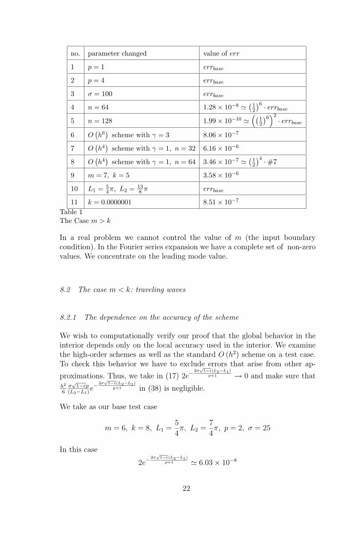
Thus, our high-order schemes should yield good results. In Table 2 we see thevalue of err = ‖uexact − φ‖∞ resulting from the use of the schemes: PT (22),HO-4 (23) and HO-6 (24). Increasing the value of n decreases the value of thegridsize h in both directions. We assume that for small values of h,

err ' C (k) n−r =C (k)

πrhr

where r is the order of the scheme, i.e.

r =

2 for PT scheme

4 for the schemes EB,HO

6 for the schemes EB-6,HO-6

Hence, if n = 2l

− log2 (err) ' l · r − log2 C (k) .

We calculate r, the order of accuracy, by measuring the slope of the curve (infigure 12). This computationally verifies our hypothesis.

23

Fig. 12. − log(err) by log(n) for the finite differences schemes

The computing time required for all of these scheme, applied on a given prob-lem, is the same when we use Gaussian elimination. This fact emphasizes thebenefit of using the high order schemes.

8.2.2 Convergence to the modified solution

We wish to confirm the modified equation’s solution (37) which we labeleduN−pml. We start with the O (h4) approximation with γ = 0, and solve theproblem with

m = 1, k = 5, L1 =5

4π, L2 =

3

2π, p = 2, σ = 20.

In this case the lower error bound is rather poor and we get

2e−2σ√

1−ε(L2−L1)

p+1 ' 7× 10−5.

Let φ be the computational approximation, uexact be the exact solution to thecombined Helmholtz-PML problem and uNPML given by (37). We measuretwo kinds of errors

errex = ‖uexact − φ‖∞and

errho = ‖uN−pml − φ‖∞Our goal is to show that the scheme converges to the uN−pml solution withO (h4). We collect the results in Table 3. We see that the scheme approximatesthe uN−pml solution and

errho (n = 32)

errho (n = 16)' errho (n = 64)

errho (n = 32)' errho (n = 128)

errho (n = 64)'(

1

2

)−4

24

n errex errho

16 3.05× 10−2 3.04× 10−2

32 2.00× 10−3 1.93× 10−3

64 1.85× 10−4 1.19× 10−4

128 7.67× 10−5 7.41× 10−6

Table 3Convergence to uho for m=1, k=5, L1 = 5

4π, L2 = 32π, p=2, σ=20 with HO-4 scheme

n errex errho

16 6.19× 10−3 6.12× 10−3

32 5.64× 10−4 4.93× 10−4

64 9.91× 10−5 2.88× 10−5

128 7.18× 10−5 1.76× 10−6


4π, L2 = 32π, p=2, σ=20 with HO-6 scheme

n errex = errho

16 1.81× 10−3

32 6.29× 10−5

64 3.33× 10−6

128 1.99× 10−7


4π, L2 =2π, p=2, σ=20 with HO-6 scheme

which is consistent with our analysis. The analytic solution is uexact. To con-

verge to uexact we set the parameters such that the exponent 2e−2σ√

1−ε(L2−L1)

p+1

is small enough.

We solve the same problem with the O (h6) scheme with γ = 0 (results inTable 4). Again, we see that we approach uN−pml and not uexact, but this time

we do not get a O (h6) approximation. For instance errho(n=64)errho(n=32)

'(

12

)−4and

not(

12

)−6. To find the cause we change L2 to 2π, to achieve better damping

in the PML. (Table 5). This time errho(n=64)errho(n=32)

'(

12

)−4.48, and in other problems

(last subsection) we do get O (h6) . The problem is that the evaluated uN−pml

is not what we are approximating in the O (h6) scheme. In the analysis of themodified equation we approximated the O (h2) term and neglected the O (h4)

25

n errex = errho

16 4.77× 10−3

32 1.15× 10−5

64 1.87× 10−7

128 2.98× 10−9

Table 6Convergence to uho for m = 1, k = 5, L1 = 5

4π, L2 = 74π, p = 4, σ = 200 with HO-6

scheme

term. However, this high order term is significant in some problems and inothers is negligible. Choosing p = 2 can be accurate for some problems (seeTable 2), however, we should choose p ≥ 4 for the O (h6) scheme. For instancein Table 6 , we do get the desired approximation

errho (n = 64)

errho (n = 32)' errho (n = 128)

errho (n = 64)'(

1

2

)−6

.

8.2.3 Selecting the parameters in the function σx

We wish to check the influence of the parameters we choose in the approxi-mation, L1, L2 − L1, p and σ, on a given problem.

8.2.3.1 Value of L1 : The error estimates we obtained imply that thevalue of L1 is relatively unimportant (we approximated | 2

η−1| that depends on

L1 by | 2η|). We check this with the test case

m = 1, k = 10, L1 − L2 =π

4, p = 4, σ = 100,

n = 32, O(h6)

scheme with γ = 0.

The value of∣∣∣ 2η

∣∣∣ = 2e−2σ√

1−ε(L2−L1)

p+1 ' 5.36× 10−14. We summarize the resultsin Table 7.

8.2.3.2 Width of the PML, L2 − L1 : To support our theory we showthat the accuracy increases as we take a thicker PML layer. Taking

m = 1, k = 10, L1 =5π

4, p = 4, σ = 100, O

(h6)

scheme with γ = 0, (41)

26

L1

∣∣∣ 2η−1

∣∣∣ err

1 4.91× 10−14 3.01× 10−3

1.25 4.73× 10−14 3.33× 10−3

1.5 4.53× 10−14 2.85× 10−3

1.75 4.30× 10−14 3.44× 10−3

2 4.03× 10−14 2.68× 10−3

2.25 3.75× 10−14 3.54× 10−3

2.5 3.44× 10−14 2.50× 10−3

Table 7The error dependance on the value of L1

L2 − L1 2e− 2σ

√1−ε(L2−L1)

p+1err

n = 32

err

n = 64π16 8.08× 10−4 3.13× 10−1 8.53× 10−3

π8 3.26× 10−7 5.92× 10−2 6.08× 10−5

π4 5.31× 10−14 3.33× 10−3 3.34× 10−5

π2 1.41× 10−27 2.16× 10−3 3.33× 10−5

π 9.98× 10−55 2.16× 10−3 3.33× 10−5

Table 8The error in the HO-6 scheme as a function of the width of the PML

L2 − L1 k = 2.5 k = 5 k = 13π16 1.68× 10−1 2.42× 10−1 4.21× 10−1

π8 1.34× 10−2 2.16× 10−2 1.10× 10−1

π4 5.16× 10−5 1.78× 10−4 1.26× 10−2

π2 1.03× 10−7 1.23× 10−5 1.44× 10−2

π 1.80× 10−8 1.24× 10−5 1.44× 10−2

Table 9The error in the HO-6 scheme as a function of width of PML and k, for n = 32

we summarize the results in Table 8. We verify that as the mesh becomesfiner we maintain the O (h6) accuracy if the PML is thick enough. Increasingthe width of the PML beyond a certain limit does not improve the accuracywhile requiring more storage and computational time. For small values of hwe obtain more accurate results, but need a thicker PML as seen in Table 9.

Our main interest is to take a thin PML, while maintaining the accuracy. We

control this by increasing the value of σ. In Table 10 we set 2e−2σ√

1−ε(L2−L1)

p+1 =

27

L2 − L1 σerr

n = 32

err

n = 64π8 400 1.7× 10−1 9.73× 10−4

π4 200 5.04× 10−3 3.36× 10−5

π2 100 2.16× 10−3 3.33× 10−5

π 50 2.16× 10−3 3.33× 10−5

Table 10The error in the HO-6 scheme for a constant value of 2e

− 2σ√

1−ε(L2−L1)

p+1

n σ L2 − L1 HO-4 HO-6

16 18.75 π2 9.66× 10−1 1.40× 10−1

32 37.5 π4 5.15× 10−2 3.02× 10−3

64 75 π8 3.62× 10−4 9.16× 10−4

Table 11Results for 8 points inside the PML with m=2, k=10, L1 = 5π

4 , p=2, σ(L2−L1)p+1 = 25π

8

n σ L2 − L1 HO-4 HO-6

16 31.25 π2 1.06× 100 1.08× 10−1

32 62.5 π4 5.14× 10−2 1.79× 10−3

64 125 π8 3.14× 10−3 7.83× 10−5

Table 12Results for 8 points inside the PML m=2, k=10, L1 = 5π

4 , p=4, σ(L2−L1)p+1 = 25π

8

1.41× 10−27 for the test problem (41). We conclude that as long as the PMLis not too thin and we have enough points in the PML, we get the desiredaccuracy.

8.2.3.3 Fixed number of points in the PML: Computational practice,is to set a fixed number of points inside the PML. Thus, when we decrease thegridsize, we change the physical width of the PML. In the above computationswe choose the physical width of the PML as constant. We want to see if thisinfluences our results. To check the behavior we set a problem with

m = 2, k = 10, L1 =5π

4

and for different values of gridsize h, use the same number of points inside thePML. In the first test (tables 11 - 13) we use 8 points in the PML, and inthe second test (Table 14 and 15) 16 points. We see that we lose the O (h6)accuracy when p = 2 (tables 11 and 14), but maintain the O (h4) behavior.

28

n σ L2 − L1 HO-4 HO-6

16 18.75 π2 1.01× 100 1.34× 10−1

32 37.5 π4 5.16× 10−2 1.64× 10−3

64 75 π8 3.17× 10−3

3.06× 10−5

(2.55× 10−5 towards uN−pml)Table 13Results for 8 points inside the PML. m=2, k=10, L1 = 5π

4 , p=4, σ(L2−L1)p+1 = 15π

8

n σ L2 − L1 HO-4 HO-6

16 9.375 π 9.94× 10−1 1.23× 10−1

32 18.75 π2 5.16× 10−2 1.67× 10−3

64 37.5 π4 3.21× 10−3 1.19× 10−4

Table 14Results for 16 points inside PML with m=2, k=10, L1 = 5π

4 , p=2, σ(L2−L1)p+1 = 25π

8

n σ L2 − L1 HO-4 HO-6

16 15.625 π 9.94× 10−1 1.24× 10−1

32 31.25 π2 5.17× 10−2 1.65× 10−3

64 62.5 π4 3.17× 10−3 2.52× 10−5

Table 15Results for 16 points inside the PML with m=2, k=10, L1 = 5π

4 , p=4, σ(L2−L1)p+1 = 25π

8

This is because for the O (h6) scheme we have to choose p ≥ 4 and havea sufficiently wide layer (compare with the results in the last section). Forthin PML layers it is noticed (Table 12) that we cannot maintain the O (h6)behavior if we choose a large σ, but by taking smaller value of σ we lose theapproximation to uexact and maintain the O (h6) accuracy towards the modifiedequation solution uN−pml. Thus, if we wish to work with a fixed number of

points inside the PML we should set the parameters such that 2e−2σ√

1−ε(L2−L1)

p+1

is small enough and choose p ≥ 4 for HO-6 and p = 2 for HO-4.

We denote n pml as the number of points in the PML

2e−2σ√

1−ε(L2−L1)

p+1 = 2e−2h·n pml·σ

√1−ε

p+1 .

If we know the minimal value of h a priori (In tables 11-15 it is π64

), we can

set n pml and σ to satisfy a desired estimate for 2e−2h·n pml·σ

√1−ε

p+1 . Hence, whenwe refine the interior grid to increase the accuracy we also need more pointsin the PML.

29

k 8 7 6.5 6.25 6.1 6.05

error 6.86 10−04 2.44 10−04 1.16 10−04 .00138 .0182 .069Table 16m = 6 and k approaches m with L1 = 5π

4 , L2 = 7π4 , σ = 25 with 32 points

pestimate

(17)

err

n = 32

err

n = 64

err

n = 128err32err64

err64err128

1 1.32× 10−68 1.19× 10−1 2.08× 10−2 4.86× 10−3 5.7 2.1

2 1.12× 10−45 1.98× 10−3 7.70× 10−5 7.59× 10−6 25.7 25.1

3 2.30× 10−34 2.22× 10−3 3.50× 10−5 6.21× 10−7 63.4 56.3

4 1.41× 10−27 2.16× 10−3 3.33× 10−5 5.21× 10−5 64.9 63.9

5 4.74× 10−23 2.16× 10−3 3.33× 10−5 5.21× 10−5 64.9 63.9

10 4.56× 10−13 2.02× 10−3 3.33× 10−5 5.21× 10−5 61.2 63.9

30 8.35× 10−5 7.23× 10−2 5.24× 10−4 7.69× 10−4 138.0 < 1Table 17Results for different values of p for m = 1, k = 10, L1 = 5π

4 , L2 = 7π4 , σ =

100, O(h6)with γ = 0

As m and k get closer we approach the evanescent limit and the PML is lesseffective. The error is shown in table (16).

8.2.3.4 Value of p : We solve the test problem with various values of p(Table 17) with

m = 1, k = 10, L1 =5π

4, L2 =

7π

4, σ = 100, O

(h6)

scheme with γ = 0.

We clearly see the bad behavior of the case p = 1 and the need for sufficientderivatives in Sx as seen in Figures 8-11. In the O (h6) case we should choosep ≥ 4. Moreover, we do not benefit from taking larger values of p than four.

8.2.3.5 Value of σ : Taking as a test problem with various values of σ,

m = 1, k = 10, L1 =5π

4, L2 =

3π

2, p = 4, O

(h6)

scheme with γ = 0.

We present the results in Table 18. We conclude that the value of σ does not

30

σestimate

(17)

err

n = 32

err

n = 64

err

n = 128err32err64

err64err128

10 8.77× 10−2 9.54× 10−2 9.23× 10−2 9.16× 10−2 1.0 1.0

20 3.85× 10−3 4.59× 10−3 3.94× 10−3 3.88× 10−3 1.2 1.0

40 7.43× 10−6 2.03× 10−3 3.39× 10−5 7.43× 10−6 59.8 4.6

80 2.75× 10−11 3.24× 10−3 3.34× 10−5 5.21× 10−7 97 64.1

160 3.81× 10−22 9.28× 10−3 3.35× 10−5 5.21× 10−7 277 64.3

320 7.25× 10−44 1.20× 10−2 3.42× 10−5 5.30× 10−7 350 64.5

103 1.31× 10−136 3.63× 10−2 4.21× 10−5 5.89× 10−7 86.6 71.5Table 18Results for different values of σ for m=1, k=10, L1 = 5π

4 , L2 = 3π2 , p=4, O

(h6)γ=0

g -10 -6 -4 -3 -1 0

err 2.73 10−3 6.75 10−4 6.66 10−4 6.70 10−4 6.81 10−4 6.86 10−4

g 1 3 4 5 6 10

err 6.87 10−4 6.83 10−4 6.76 10−4 6.68 10−4 6.72 10−4 2.72 10−3

Table 19Error varying g in Sx =1 + σx

g+ik . L1 = 5π4 , L2 = 7π

4 , m=6, k=8, 32 points, σ= 25

influence the accuracy of the approximation as long as 2e−2σ√

1−ε(L2−L1)

p+1 is smallenough. Thus, a natural choice of σ should be σ > k such that

2e−2σ√

1−ε(L2−L1)

p+1 ˜10−q

where q is the number of the desired significant digits accuracy. We choose thesmallest σ that satisfies this.

We next consider a more general formula for Sx given by Sx = 1 + σx

g+ik. The

original formula corresponds to g = 0. In table (19) we present the error as afunction of g. We consider L1 = 5π

4, L2 = 7π

4, m = 6, k = 8 with 32 points and

σ = 25. We see that indeed the smallest error occurs for g = −5.0. However,the differences are so small that there is no practical purpose in trying tochoose a nonzero g. Hence, we continue to use the original g = 0.

9 Iterative Techniques

For very fine meshes in two dimensions and coarser meshes in three dimensionsan LU decomposition becomes very expensive. Hence, we consider the use of

31

an iterative solver. We examine Krylov subspaces methods such as CGNR,GMRES, QMR and BiCG on the combined problem and found that theyconverge to the solution very slowly. Hence, we need to use a preconditionerfor the problem. A preconditioner for the pure Helmholtz equation was con-structed in [3]. The preconditioner was based on the inverse of the Laplacianoperator computed with one sweep of SSOR.

The major difficulty of this preconditioner on the combined problem is thatthe PML introduces a different equation. k = 0 in the PML does not givethe Laplace equation. Instead, we construct a preconditioner, that will act asthe inverse Laplacian operator in the interior, and behave as an approximateinverse in the PML. We do not calculate M−1 but we approximate the solutionof My = z, by applying a few sweeps of SSOR or damped Jacobi (DJ). In thePML we cannot choose k = 0 because of the definition of Sx. For the Helmholtzequation with small but nonzero k the operator is still positive definite. Thus,to apply the preconditioner M we use the standard approximation of thecombined problem with a small value of k which we denote k.

αDx (Aux)j +1− α

2(Dx (Aux)j+1 + Dx (Aux)j−1) +

αDy (Buy)i +1− α

2(Dy (Auy)i+1 + Dy (Auy)i−1) +

(1− 4βs − 4βc) Ci,jui,j

+βs

Ci+1,jui+1,j + Ci−1,jui−1,j+

Ci,j+1ui,j+1 + Ci,j−1ui,j−1

+βs

Ci+1,j+1ui+1,j+1 + Ci−1,j+1ui−1,j+1+

Ci+1,j−1ui+1,j−1 + Ci−1,j−1ui−1,j−1

.

Where A = 1Sx

, B = Sx, C = k2Sx. The resulting matrix M is complex andcannot be applied as a preconditioner for two reasons. It is not symmetric andit is not real and positive definite. It does have these two properties in theinterior, but not in the PML.

To overcome these two difficulties we set the PT values: α=1, βs =βc =0 inthe preconditioner. This choice makes the approximation complex-symmetric.It is also useful because it involves only 5 unknowns in each equation insteadof 9. To change the matrix to a real symmetric positive definite matrix wemake the change:

Mi,j =

∣∣∣Mi,j

∣∣∣ i = j

−∣∣∣Mi,j

∣∣∣ i 6= jfor every 1 ≤ i, j ≤ N.

32

nσ = 10

p = 1

σ = 10

p = 2

σ = 1

p = 4

σ = 10

p = 4

σ = 100

p = 4

σ = 10

p = 6

16 211 206 208 200 204 204

32 832 811 927 807 807 871

64 4022 3911 4683 3766 3857 4421Table 20Number of iterations in the Left Preconditioned CGNR with diagonal scaling using4 sweeps of DJ with ω = 0.7 applied on the combined preconditioner with k = 0.1.

n with diagonal scaling without diagonal scaling

16 351 877

32 1732 12823

64 8646 116744Table 21Number of iterations non preconditioned CGNR with and without diagonal scaling

In the interior Mi,j = Mi,j. Because k is small in the interior, the approxima-tion is a small perturbation of the Laplacian. We call this preconditioner thecombined preconditioner. Note, that as in the pure Laplacian operator precon-ditioner, this preconditioner corresponds to a second order accurate operatoreven when the scheme in the interior is higher order accurate.

Table 20 shows the number of iterations for the CGNR preconditioned algo-rithm with the new combined preconditioner. We choose k = 0.1. The bestvalue of p in the preconditioner is the same as used for the approximation.σ should be small, but not too small. The benefit of the preconditioner isdemonstrated comparing the convergence with that of the non-preconditionedalgorithm in Table 21. As shown in [3] as k gets larger the preconditioner isless effective. This can be improved as in [15].

10 Conclusions

We construct a PML for the two dimensional Helmholtz equation in a strip.We prove that the combined Helmholtz and PML layer has a unique solutionand that this solution is a good approximation to the interior Helmholtz equa-tion. We find a bound for this error and show that one can control the errorby changing the PML parameters. We describe high-order finite differencesschemes for the combined Helmholtz PML equation and apply them on thestrip problem. We analyze the numerical error governed by the use of theseschemes and show that for a proper choice of parameters, the combined scheme

33

maintains the high-order accuracy of the interior approximation. A variety ofnumerical results is presented to support the analysis.

We also investigate the use of iterative methods to solve the resultant linearequations. We develop a preconditioner Krylov algorithms to solve the com-bined problem. We conclude that the parameters should be chosen so that:

• The length of the interior, L1, should be as small as the physical problempermits because it does not influence the accuracy but has a significantimpact on the size of the linear system.

• The width of the PML, L2 − L1, should be as thin as possible to decreasethe size of the linear system. Numerical tests show that we cannot makethe layer too thin relative to the interior grid. For the interior grids used inthis study we could use 16 grid points in the PML and still get high orderaccuracy. If the grid is refined than one needs more points in the PML.

• The degree of the polynomial in the PML, p, (see (14)) should be 2 for thefourth order accurate scheme and 4 for the sixth order accurate scheme.

• σ, the maximum of σx (x) (see (14)) should be set to the lowest value which

maintains the desired accuracy determined by e−2σ√

1−ε(L2−L1)

p+1 (see (17)).• If both travelling and evanescent waves are present then the size of the PML

should be chosen to damp the evanescent waves. Then the other parametersare chosen to efficiently damp the traveling waves. The difficult situation istravelling waves near resonance.

34

References

[1] S. Abarbanel and D. Gottlieb, A Mathematical Analysis of the PML Method,J. Comput. Physics, 134, 357-363 (1997).

[2] A. Bayliss, C.I. Goldstein and E.Turkel, An Iterative Method for the HelmholtzEquation, J. Comput. Physics 49, 443-457 (1983).

[3] A. Bayliss, C.I. Goldstein and E.Turkel, Preconditioned Conjugate-GradientMethods for the Helmholtz Equation, Elliptic Problem Solvers II , 233-243(1984).

[4] A. Bayliss, M. Gunzburger, E. Turkel, Boundary Conditions for the NumericalSolution of Elliptic Equations in Exterior Regions, SIAM J. Appl. Math. 42,430-45l (1982).

[5] J-P Berenger, A Perfectly Matched Layer for the Absorption of ElectromagneticWaves, J. Comput. Physics, 114, 185-200 (1994).

[6] J-P Berenger, Three Dimensions Perfectly Matched Layer for the Absorption ofElectromagnetic Waves, J. Comput. Physics, 127, 363-379 (1996).

[7] A. Greenbaum, Iterative Methods for Solving Linear Systems, SIAM,Philadelphia (1997).

[8] S. Gedney, The Perfectly Matched Layer Absorbing Media, Advances inComputational Electrodynamics: The Finite-Difference Time-Domain Method,A. Taflove editor, Artech House 263-343 (1998).

[9] I. Harari and E. Turkel, Accurate Finite Difference Methods for Time-HarmonicWave Propagation, J. Comput. Physics, 119, 252-270 (1995).

[10] P.G. Petropoulos, On the Termination of the Perfectly Matched Layer with LocalAbsorbing Boundary Conditions, J. Comput. Physics, 143, 665-673 (1968).

[11] I. Singer and E. Turkel, High Order Finite Difference Methods for the HelmholtzEquation, Comput. Methods Appl. Mech. Eng. 163, 343-358 (1998).

[12] I. Singer and E. Turkel, Sixth Order Accurate Finite Difference Schemes for theHelmholtz Equation submitted to Journal of Computational Acoustics.

[13] S. Tsynkov and E. Turkel, A Cartesian Perfectly Matched Layer for theHelmholtz Equation, Artificial Boundary Conditions with Applications to CEM,Loic Tourrette editor, Novascience Publishing (2001).

[14] E. Turkel, Numerical Difficulties Solving Time Harmonic Equations, MultiscaleComputational Methods in Chemistry and Physics, A. Brandt, J. Bernholc andK. Binder editors, IOS Press, Ohmsha, 319-337 (2001).

[15] C. Vuik, Y.A. Erlangaa and C.W. Oosterlee. Shifted Laplace preconditioners forthe Helmholtz Equation, ENUMATH 2003.

[16] E. Turkel and A. Yefet, Absorbing PML Boundary Layers for Wave-LikeEquations, Appl. Numer. Math. 27, 533-557 (1998).

35

A Perfectly Matched Layer for the Helmholtz Equation in a ...turkel/PSmanuscripts/ido_pml.pdf ·...

Documents

Transcript of A Perfectly Matched Layer for the Helmholtz Equation in a ...turkel/PSmanuscripts/ido_pml.pdf ·...