A Particle Filter Framework for Contour Detection

A Particle Filter Framework for Contour Detection

Nicolas Widynski and Max Mignotte

Department of Computer Science and Operations Research (DIRO), University of Montreal,C.P. 6128, succ. Centre-Ville, , Montreal (Quebec), H3C 3J7, Canada

widynski,[email protected]

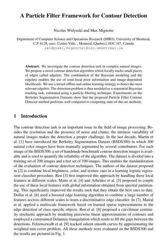
Abstract. We investigate the contour detection task in complex natural images.We propose a novel contour detection algorithm which locally tracks small piecesof edges called edgelets. The combination of the Bayesian modeling and theedgelets enables the use of semi-local prior information and image-dependentlikelihoods. We use a mixed offline and online learning strategy to detect the mostrelevant edgelets. The detection problem is then modeled as a sequential Bayesiantracking task, estimated using a particle filtering technique. Experiments on theBerkeley Segmentation Datasets show that the proposed Particle Filter ContourDetector method performs well compared to competing state-of-the-art methods.

1 Introduction

The contour detection task is an important issue in the field of image processing. Be-sides the resolution and the presence of noise and clutter, the intrinsic variability ofnatural images makes the detection a proper challenge. In the last decade, Martin etal. [1] have introduced the Berkeley Segmentation Dataset (BSDS300) in which 300natural color images have been manually segmented by several contributors. For eachimage of the BSDS300, a set of handmade benchmark contour detection images is avail-able and is used to quantify the reliability of the algorithm. The dataset is divided into atraining set of 200 images and a test set of 100 images. This enables the standardizationof the evaluation of contour detection techniques. The authors of the dataset proposedin [2] to combine local brightness, color, and texture cues in a learning logistic regres-sion classifier procedure. Ren [3] first improved this approach by handling these localfeatures at different scales. Maire et al. [4] and Arbelaez et al. [5] proposed to couplethe use of these local features with global information obtained from spectral partition-ing. This significantly improved the results such that they obtain the best ones to date.Dollar et al. [6] used a boosted edge learning algorithm to combine a large number offeatures accross different scales to learn a discriminative edge classifier. In [7], Mairalet al. applied a multiscale framework based on learned sparse representations to theedge detection of class-specific objects. Ren et al. [8] proposed a curvilinear continu-ity stochastic approach by modeling piecewise linear approximations of contours andemployed a constrained Delaunay triangulation which tends to fill the gaps between thedetections. Felzenszwalb et al. [9] tracked salient smooth curves by approximating theweighted min-cover problem. All these methods were evaluated on the BSDS300 andthe results are pictured in Fig. 1.

2 Nicolas Widynski, Max Mignotte

1

0.8

0.7

0.6

0.5

0.4

0.3

0.2

0.1

00 0.1 0.2 0.3 0.4 0.5 0.6 0.7 0.8 0.9 1

0.1

0.9

0.2

0.3

0.4

0.5

0.6

0.7

0.8

0.9

iso-F

Recall

Pre

cisi

on

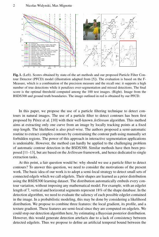
[F = 0.79] Human[F = 0.70] gPb - Maire, Arbeláez, Fowlkes, Malik (2008)

[F = 0.68] Multiscale - Ren (2008)[F = 0.66] BEL - Dollar, Tu, Belongie (2006)[F = 0.66] Mairal, Leordeanu, Bach, Herbert, Ponce (2008)[F = 0.65] Min Cover - Felzenszwalb, McAllester (2006)[F = 0.65] Pb - Martin, Fowlkes, Malik (2004)[F = 0.64] Untangling Cycles - Zhu, Song, Shi (2007)[F = 0.64] CRF - Ren, Fowlkes, Malik (2005)[F = 0.58] Canny (1986)[F = 0.56] Perona, Malik (1990)[F = 0.50] Hildreth, Marr (1980)[F = 0.48] Prewitt (1970)[F = 0.48] Sobel (1968)[F = 0.47] Roberts (1965)

[F = 0.68] Particle Filter Contour Detector (PFCD)

Fig. 1. (Left). Scores obtained by state-of-the art methods and our proposed Particle Filter Con-tour Detector (PFCD) model (illustration adapted from [5]). The evaluation is based on the F-Measure, which is a combination of the precision measure and the recall one: it supports a highnumber of true detections while it penalizes over-segmentation and missed detections. The finalscore is the optimal threshold computed among the 100 test images. (Right). Image from theBSDS300 and ground truth boundaries. The image outlined in red is obtained by our PFCD.

In this paper, we propose the use of a particle filtering technique to detect con-tours in natural images. The use of a particle filter to detect contours has been firstproposed by Perez et al. [10] with their well-known JetStream algorithm. This methodaims at extracting only one curve from an image by locally tracking points at a fixedstep length. The likelihood is also pixel-wise. The authors proposed a semi-automaticroutine to extract complex contours by constraining the contour path using manually setforbidden regions. The power of this approach in interactive segmentation applicationsis undeniable. However, the method can hardly be applied to the challenging problemof automatic contour detection in the BSDS300. Similar methods have then been pro-posed [11–13], but are based on the JetStream framework, and hence dedicated to singleextraction tasks.

At this point, a fair question would be: why should we use a particle filter to detectcontours? To answer this question, we need to consider the motivations of the presentwork. The basic idea of our work is to adopt a semi-local strategy to detect small sets ofconnected edgels which we call edgelets. Their shapes are learned as a prior distributionusing the BSDS300 learning dataset. The distribution automatically embeds every con-tour variation, without imposing any mathematical model. For example, with an edgeletlength of 7, vertical and horizontal segments represent 18% of the shape database. In thedetection algorithm, we need to evaluate the saliency of each possible edgelet containedin the image. In a probabilistic modeling, this may be done by considering a likelihooddistribution. We propose to combine three features: the local gradient, its profile, and atexture gradient. These features are semi-local since they are computed on edgelets. Wecould stop our detection algorithm here, by estimating a Bayesian posterior distribution.However, this would generate detection artefacts due to a lack of consistency betweendetected edgelets. Thus we propose to define an artificial temporal bound between the

A Particle Filter Framework for Contour Detection 3

∀n ∈ 1, . . . , N,

fcheck

et; e

(n)1:t−1

∀t ∈ 1, . . . , T,

e(n)t−1

Init

Transition

Local gradient

Textural gradient

Profile gradient

Prior

Transition with

Initialization:

Learning

Weighting

Proposition

w(n)t = PastWeight× Likelihood× Prediction

Proposition

= w(n)t−1

p(yt|e(n)t ) p(e

(n)t |e(n)

t−1, c(n)t ) p(c

(n)t )

q(e(n)t | . . . ) q(c

(n)t | . . . )

p(e0|y0)

∝ Likelihood× Prior

= p(y0|e0)× p(e0)

p(yj0|e0) ∝ exp

− λjP (µj > fj(e0,y

j0)

p(y0|e0) =

J

j=1

p(yj0|e0)p(e

(j)t |e(i)

t−1)

e(j)t

e(i)t−1

P (µ1 > f1(e(k)0 ,y1

0))

P (µ2 > f2(e(k)0 ,y2

0))

P (µ3 > f3(e(k)0 ,y3

0))

Output

e = (e1, . . . , e7)

e(i) p(e(i))

Offline Online

Tracking

Feature distributions:

c(n)t ∼

e(n)t ∼

q(ct| . . . ) =

consistency check of the trajectory

q(et| . . . ) =

Init p(et|y0) if c

(n)t = jump,

Transition p(et|e(n)t−1) otherwise.

×

Approximation of the posterior distribution

p(e0:t, c0:t|y0:t) ≈N

n=1

w(n)t δ

e(n)0:t

e0:t δc(n)0:t

c0:t

α =

j λj P (µj > fj(et−1,y

jt−1)) if ct = jump,

1− α otherwise.

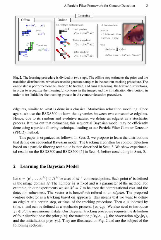
Fig. 2. The learning procedure is divided in two steps. The offline step estimates the prior and thetransition distributions, which are used to generate samples in the contour tracking procedure. Theonline step is performed on the image to be tracked, and aims at learning: the feature distributions,in order to recognize the meaningful contours in the image; and the initialization distribution, inorder to (re-)initialize the tracking process in the contour detection procedure.

edgelets, similar to what is done in a classical Markovian relaxation modeling. Onceagain, we use the BSDS300 to learn the dynamics between two consecutive edgelets.Hence, due to its random and evolutive nature, we define an edgelet as a stochasticprocess. It turns out that estimating this sequential Bayesian model may be efficientlydone using a particle filtering technique, leading to our Particle Filter Contour Detector(PFCD) method.

This paper is organized as follows. In Sect. 2, we propose to learn the distributionsthat define our sequential Bayesian model. The tracking algorithm for contour detectionbased on a particle filtering technique is then described in Sect. 3. We show experimen-tal results on the BSDS300 and BSDS500 [5] in Sect. 4, before concluding in Sect. 5.

2 Learning the Bayesian Model

Let e = (e1, . . . , eM ) ∈ ΩM be a set ofM 4-connected points. Each point ei is definedin the image domain Ω. The number M is fixed and is a parameter of the method. Forexemple, in our experiments we set M = 7 to balance the computational cost and thedetection robustness. The vector e is henceforth refered to an edgelet. The proposedcontour detector is a tracking based on approach. This means that we want to definean edgelet at a certain step, or time, of the tracking procedure. Then e is indexed bytime, t, and can be defined as a stochastic process, ett∈N. We also need to introduceyt ∈ Y , the measurement state. Our Bayesian tracking procedure requires the definitionof four distributions: the prior p(e), the transition p(et|et−1), the observation p(yt|et),and the initialization p(e0|y0). They are illustrated on Fig. 2 and are the subject of thefollowing sections.


Algorithm 1: Approximation of the prior distribution of an edgeletInput: A shape databaseOutput: Approximation of the prior distribution p(e2:M |e1)begin

for s = 1, . . . , Sp doSelect an image I and a segmentation H at randomExtract an edgelet e(s) from (I,H) at randomCenter it with respect to e1(s)

return 1Sp

∑Sp

s=1 δee(s)

, where δba = 1 if a = b, and 0 otherwise

Algorithm 2: Approximation of the transition distribution of an edgeletInput: Distribution p(e), a shape databaseOutput: Approximation of the transition distribution p(et|et−1)begin

foreach distinct element e′(u) ∈ e′(1), . . . , e′(S′p) ⊂ e(1), . . . , e(Sp) do

repeatSelect an image I and a segmentation H at randomExtract two consecutives edgelets from (I,H) such that et = e′(u) and

et−1 = e′(v) ∈ e′(1), . . . , e′(S′p) its predecessor

Increment by 1/St the probability p(et = e′(u)|et−1 = e′(v))until St times

2.1 Offline Learning: Prior Model

The vector e is a small piece of a contour, integrating more information than a classi-cal pixel-wise formulation. Nevertheless, it remains semi-local, in order to be appliedgenerally to most of the contours. By learning its prior distribution, we avoid impos-ing mathematical constraints that may decrease the power of detection of an algorithm,since it is impractical to define a mathematical model that captures every possible con-tour singularity. Algorithm 1 presents the offline approximation procedure of the priordistribution p(e). The parameter Sp denotes the number of samples and e(s) is the s-threalization of the approximation set. Each sample e(s) is centered with respect to its firstpoint e1(s). Using the BSDS300 training dataset, we learn the distribution p(e2:M |e1)to capture only the shapes of the edgelets.

2.2 Offline Learning: Transition Model

We defined in the previous section a way to initialize edgelets. Next, to randomly extractfull contours with our tracking algorithm, we need to generate a possible edgelet shapeat a certain time t given the previous one at t−1. This is what the transition distributionp(et|et−1) is designed to. It can be approximated using Algorithm 2. We use the sameshape dataset as in Sect. 2.1.


2.3 Online Learning: Observation Model

In this section, we define a density p(yt|et) which measures the adequation betweendata known at a time t, yt, and an edgelet et. To make our detector robust, we firstconsider several observations, i.e. yt = (y1

t , . . . ,yJt ), with yj

t ∈ Yj , each of thesebeing related to a special feature. The joint likelihood p(yt|et) is defined considering aconditional independence hypothesis of the yj

t , 1 ≤ j ≤ J , given et:

p(yt|et) =J∏

j=1

p(yjt |et) . (1)

This simplifies the estimation since we just need to define the marginal likelihoodsp(yj

t |et). The observation yjt is related to a feature fj : ΩM × Yj → R. The features

fjJj=1 are computed along an edgelet et and integrate color and gradient informationto precisely localize contours.

Before defining these features, we propose a general formulation of the densitiesp(yj

t |et). It is clear that the quantity of information of each feature depends on theimage itself. For example, a classical gradient feature typically overdetects in texturedimages whereas its sensitivity drops in blurry ones. The interpretation of the featureresponses should be different in these two cases, meaning that a candidate should bemore relevant when it obtains a singular high feature response value in the image. Thisidea has been used in an a contrario framework [14], and is related to the notion ofmeaningfulness of an event. Here, an event is an edgelet et and we want to computehow meaningful the feature response on et is on the image. This implies to learn adistribution P

(µj > fj(et,y

jt )), with µj a random variable associated to the feature

fj , in order to consider the shape of the feature response distribution into the likelihood.This distribution can be assimilated as a distribution of false alarms. Hence, the lowerthe probability P

(µj > fj(et,y

jt )), the more meaningful this event, i.e., the less likely

the event et corresponds to a false alarm. The approximation of the feature distributionis given in Algorithm 3. Finally, we define the likelihood in a way to support low valuesof P

(µj > fj(et,y

jt )):

p(yjt |et) ∝ exp

(− λj P

(µj > fj(et,y

jt )))

, (2)

with λj ∈ R+ a learned multiplicative constant value which both aims at providing agood localization of high likelihood and impacts the relevance of the feature j on thetracking procedure.

We now describe our three features: f1 the local gradient, f2 the textural gradi-ent, and f3 the profile gradient. The main novelty about the proposed features comesfrom the edgelet modeling. In particular, we are expecting to provide robust featureresponses, since they are semi-local and less dependent on noise.

Local Gradient. This classical feature uses the 2×2 gradient norm |∇I| of the image I .The gradient feature f1 is computed along an edgelet et:

f1(et,y1t ) = Φ

(( ∣∣∇I(eit)∣∣)1≤i≤M

). (3)


Algorithm 3: Approximation of the feature distributionInput: Distribution p(e), an image I : Ω → ROutput: Approximation of the feature distribution P

(µj > fj(e0,y

j0))

beginfor s = 1, . . . , Sf do

Select a starting point e1(s)0 at random: e1(s)

0 ∼ U [Ω]

Generate the edgelet shape e2:M(s)0 according to the prior distribution:

e2:M(s)0 |e1(s)

0 ∼ p(e2:M |e1)

Compute and store fj(e(s)0 ,yj

0)

return 1Sf

∑Sfs=1 1

[−∞,fj(e

(s)0 ,y

j0)](fj(e0,y

j0))

The flexibility comes from the fusion operator Φ. One can set Φ = min, Φ = max,or a weighted mean Φ(v1, . . . , vM ) =

∑Mj=1W (j) vj , with W : 1, . . . ,M → [0, 1]

a weighting function. In our experiments, we set W (j) = 1/M,∀j. Note that whenthe image I is multidimensionnal, we take on each point the maximum gradient valueamong the different channels.

Textural Gradient. The textural gradient feature aims at getting low response valueson texture locations, while getting high ones on object contours. For a point ejt of anedgelet et, we consider its normal segment. The two sides of the normal segment ofthree consecutive points (ej−1t , ejt , e

j+1t ) are noted←−n (ejt ) and −→n (ejt ). In a texture, the

intuition is that color pixel values along the first segment should not really differ fromthe ones of the second segment. Let h[a] = hr[a]Rr=1 be the histogram of a set ofpixels a, where r is the bin index of an histogram of length R. Distances between pairsof histograms along normals of the curve are combined to form the texture feature:

f2(et,y2t ) = Ψ

((dB(h[←−n (eit)], h[

−→n (eit)]))

2≤i≤M−1

), (4)

with Ψ the fusion operator, and dB the Bhattacharyya distance between two histograms,i.e., dB(h[a], h[b]) is the square root of 1−∑R

r=1

√hr[a]hr[b].

Profile Gradient. The last feature comes from a recent idea from Sun et al. [15]. Theypropose to analyse the gradient profile for image enhancement and super-resolution.This profile is learned and represented by a parametric gradient profile model. Thismodel does not use the gradient value of a contour, but the symmetry and the mono-tonicity of its profile. Thus, in our application, we expect that this feature detects sharpcontours as well as smooth ones. It can also be useful when there are instabilities in thegradient norm, due to noise, while the symmetry and the monotony of its profile shouldremain. With n(ejt ) the normal segment of three consecutive points (ej−1t , ejt , e

j+1t ),

the profile gradient feature is defined as:

f3(et,y3t ) = Ξ

((− dKL

( ∣∣∇I[n(eit)

]∣∣ , gp(n(eit)|eit, σp, λp)))

2≤i≤M−1

), (5)


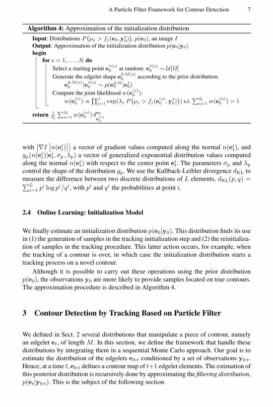
Algorithm 4: Approximation of the initialization distribution

Input: Distributions P(µj > fj(e0,y

j0)), p(e0), an image I

Output: Approximation of the initialization distribution p(e0|y0)begin

for s = 1, . . . , Si doSelect a starting point e1(s)

0 at random: e1(s)0 ∼ U [Ω]

Generate the edgelet shape e2:M(s)0 according to the prior distribution:

e2:M(s)0 |e1(s)

0 ∼ p(e2:M0 |e1

0)

Compute the joint likelihood w(e(s)0 ):

w(e(s)0 ) ∝

∏Jj=1 exp(λj P

(µj > fj(e

(s)0 ,yj

0))) s.t.

∑Siu=1 w(e

(u)0 ) = 1

return 1Si

∑Sis=1 w(e

(s)0 ) δe0

e(s)0

with∣∣∇I

[n(eit)

]∣∣ a vector of gradient values computed along the normal n(eit), andgp(n(e

it)|eit, σp, λp) a vector of generalized exponential distribution values computed

along the normal n(eit) with respect to the center point eit. The parameters σp and λpcontrol the shape of the distribution gp. We use the Kullback-Leibler divergence dKL tomeasure the difference between two discrete distributions of L elements, dKL(p, q) =∑L

i=1 pi log pi/qi, with pi and qi the probabilities at point i.

2.4 Online Learning: Initialization Model

We finally estimate an initialization distribution p(e0|y0). This distribution finds its usein (1) the generation of samples in the tracking initialization step and (2) the reinitializa-tion of samples in the tracking procedure. This latter action occurs, for example, whenthe tracking of a contour is over, in which case the initialization distribution starts atracking process on a novel contour.

Although it is possible to carry out these operations using the prior distributionp(e0), the observations y0 are more likely to provide samples located on true contours.The approximation procedure is described in Algorithm 4.

3 Contour Detection by Tracking Based on Particle Filter

We defined in Sect. 2 several distributions that manipulate a piece of contour, namelyan edgelet et, of length M . In this section, we define the framework that handle thesedistributions by integrating them in a sequential Monte Carlo approach. Our goal is toestimate the distribution of the edgelets e0:t conditioned by a set of observations y0:t.Hence, at a time t, e0:t defines a contour map of t+1 edgelet elements. The estimation ofthis posterior distribution is recursively done by approximating the filtering distribution,p(et|y0:t). This is the subject of the following section.


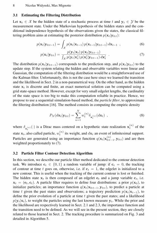
3.1 Estimating the Filtering Distribution

Let xt ∈ X be the hidden state of a stochastic process at time t and yt ∈ Y be themeasurement state. Under the Markovian hypothesis of the hidden states and the con-ditional independence hypothesis of the observations given the states, the classical fil-tering problem aims at estimating the posterior distribution p(xt|y0:t):

p(xt|y0:t−1) =∫

Xp(xt|xt−1) p(xt−1|y0:t−1) dxt−1 , (6)

p(xt|y0:t) =p(yt|xt) p(xt|y0:t−1)∫

X p(yt|x′t) p(x′t|y0:t−1) dx′t. (7)

The distribution p(xt|y0:t−1) corresponds to the prediction step, and p(xt|y0:t) to theupdate step. If the system relating the hidden and observable variables were linear andGaussian, the computation of the filtering distribution would be a straightforward use ofthe Kalman filter. Unfortunately, this is not the case here since we learned the transitionand the likelihood in Sect. 2 in a non-parametrical way. On the other hand, as the hiddenstate xt is discrete and finite, an exact numerical solution can be computed using agrid state-space method. However, except for very small edgelet lengths, the cardinalityof the state space is too big to make this computation reliable in practice. Hence, wepropose to use a sequential simulation-based method, the particle filter, to approximatethe filtering distribution [16]. The method consists in computing the empiric density

PN (dxt|y0:t) =

N∑

n=1

w(n)t δ

x(n)t

(dxt) , (8)

where δx(n)t

(·) is a Dirac mass centered on a hypothetic state realization x(n)t of the

state xt, also called particle, w(n)t its weight, and dxt an event of infinitesimal support.

Particles are generated using an importance function q(xt|x(n)0:t−1,y0:t) and are then

weighted proportionately to (7).

3.2 Particle Filter Contour Detection Algorithm

In this section, we describe our particle filter method dedicated to the contour detectiontask. We introduce ct ∈ 0, 1 a random variable of jump: if ct = 0, the trackingof contour at time t goes on, otherwise, i.e. if ct = 1, the edgelet is initialized to anew contour. This is useful when the tracking of the current contour is lost or finished.The hidden state xt is then composed of an edgelet et and a jump variable ct, i.e.xt = (et, ct). A particle filter requires to define four distributions: a prior p(x0), toinitialize particles; an importance function q(xt|x0:t−1,y0:t), to predict a particle attime t given the past states and observations; a trajectory prediction p(xt|xt−1), todefine the prior evolution of a particle at time t given the past states; and a likelihoodp(yt|xt), to weight the particles using the last known measure yt. While the prior andthe likelihood are respectively learned in Sect. 2.1 and 2.3, the importance function andthe transition need to be defined. As we will see in the present section, they are closelyrelated to those learned in Sect. 2. The tracking procedure is summarized on Fig. 3 anddetailed in Algorithm 5.


∀n ∈ 1, . . . , N,

fcheck

et; e

(n)1:t−1

∀t ∈ 1, . . . , T,

e(n)t−1

Init

Transition

Local gradient

Textural gradient

Profile gradient

Prior

Transition with

Initialization:

Learning

Weighting

Proposition

w(n)t = PastWeight× Likelihood× Prediction

Proposition

= w(n)t−1

p(yt|e(n)t ) p(e

(n)t |e(n)

t−1, c(n)t ) p(c

(n)t )

q(e(n)t | . . . ) q(c

(n)t | . . . )

p(e0|y0)

∝ Likelihood× Prior

= p(y0|e0)× p(e0)

p(yj0|e0) ∝ exp

− λjP (µj > fj(e0,y

j0)

p(y0|e0) =

J

j=1

p(yj0|e0)p(e

(j)t |e(i)

t−1)

e(j)t

e(i)t−1

P (µ1 > f1(e(k)0 ,y1

0))

P (µ2 > f2(e(k)0 ,y2

0))

P (µ3 > f3(e(k)0 ,y3

0))

Output

e = (e1, . . . , e7)

e(i) p(e(i))

Offline Online

Tracking

Feature distributions:

c(n)t ∼

e(n)t ∼

q(ct| . . . ) =

consistency check of the trajectory

q(et| . . . ) =

Init p(et|y0) if c

(n)t = jump,

Transition p(et|e(n)t−1) otherwise.

×

Approximation of the posterior distribution

p(e0:t, c0:t|y0:t) ≈N

n=1

w(n)t δ

e(n)0:t

e0:t δc(n)0:t

c0:t

α =

j λj P (µj > fj(et−1,y

jt−1)) if ct = jump,

1− α otherwise.

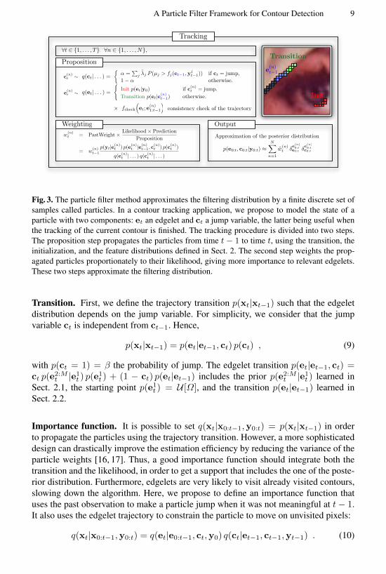
Fig. 3. The particle filter method approximates the filtering distribution by a finite discrete set ofsamples called particles. In a contour tracking application, we propose to model the state of aparticle with two components: et an edgelet and ct a jump variable, the latter being useful whenthe tracking of the current contour is finished. The tracking procedure is divided into two steps.The proposition step propagates the particles from time t − 1 to time t, using the transition, theinitialization, and the feature distributions defined in Sect. 2. The second step weights the prop-agated particles proportionately to their likelihood, giving more importance to relevant edgelets.These two steps approximate the filtering distribution.

Transition. First, we define the trajectory transition p(xt|xt−1) such that the edgeletdistribution depends on the jump variable. For simplicity, we consider that the jumpvariable ct is independent from ct−1. Hence,

p(xt|xt−1) = p(et|et−1, ct) p(ct) , (9)

with p(ct = 1) = β the probability of jump. The edgelet transition p(et|et−1, ct) =ct p(e

2:Mt |e1t ) p(e1t ) + (1 − ct) p(et|et−1) includes the prior p(e2:Mt |e1t ) learned in

Sect. 2.1, the starting point p(e1t ) = U [Ω], and the transition p(et|et−1) learned inSect. 2.2.

Importance function. It is possible to set q(xt|x0:t−1,y0:t) = p(xt|xt−1) in orderto propagate the particles using the trajectory transition. However, a more sophisticateddesign can drastically improve the estimation efficiency by reducing the variance of theparticle weights [16, 17]. Thus, a good importance function should integrate both thetransition and the likelihood, in order to get a support that includes the one of the poste-rior distribution. Furthermore, edgelets are very likely to visit already visited contours,slowing down the algorithm. Here, we propose to define an importance function thatuses the past observation to make a particle jump when it was not meaningful at t− 1.It also uses the edgelet trajectory to constrain the particle to move on unvisited pixels:

q(xt|x0:t−1,y0:t) = q(et|e0:t−1, ct,y0) q(ct|et−1, ct−1,yt−1) . (10)


The distribution q(ct|et−1, ct−1,yt−1) is set to (1− ct)(1− α) + ct α. The value α isthe probability to jump to an unexplored contour, and depends on how much meaningfulthe past edgelet et−1 was according to the J feature distributions:

α =

J∑

j=1

λj P (µj > fj(et−1,yjt−1)) , (11)

with λj the normalized value of λj of (2). The edgelet importance function includesa trajectory constraint fcheck as well as the transition and initialization distributionsrespectively learned in Sect. 2.2 and 2.4:

q(et|e0:t−1, ct,y0) = nq fcheck(et, et−1, e0:t−2)[ct p(et|y0) + (1− ct) p(et|et−1)

].

(12)

The trajectory constraint fcheck(·) is set to 0 if any point in the edgelet et go throughany point of et−1 or is closer than a Manhattan distance of 2 with any point of thepast trajectory e0:t−2. This is done to prevent an echo detection effect. Otherwise weset fcheck(·) = 1. Generating particles according to (12) can be done using a rejectionsampling: a sample e(n)t is generated according to c

(n)t p(et|y0)+(1−c

(n)t ) p(et|et−1)

and accepted with a probability of fcheck(e(n)t , e

(n)t−1, e

(n)0:t−2). Finally, the normaliz-

ing constant nq is approximated using an importance sampling method, i.e. nq ≈1Nq

∑Nq

i=1 fcheck(e(i)t , et−1, e0:t−2), with e

(i)t ∼ p(et|et−1, ct).

Stopping Criterion. We discussed how to init and iterate the tracking algorithm, butthe question of its stopping remains. The easiest way is based on the fact that the al-gorithm first tracks the most meaningful contours. This is due to the resampling tech-nique used in the particle filters, which duplicates the good particles and discards thebad ones. Then, according to the feature distributions, detected contours become lessand less meaningful, and one may stop the algorithm when the meaningfulness reachesa given threshold. In particular, we defined in (11) the probability of jump using themeaningfulness of an edgelet, and this probability grows with time. Then, we stop aparticle filter when the proportion of jumps reaches a fixed threshold:

1

K + 1

K∑

k=0

N∑

n=1

w(n)t c

(n)t−k ≥ γ . (13)

Diversity. A resampling technique is used to avoid a degeneracy problem (all the par-ticles but one converge to zero after a few steps), inherent to the particle filtering tech-nique [16, 17]. This does not alter the posterior distribution but impacts on the diversityof the particles, especially for the past states. In practice, this means that most of theparticles share the same trajectory, which may degrade the quality of the estimator. Toalleviate this effect, we propose to divide the NL particles into L independent particlefilters, leading to the following final posterior distribution:

p(x0:t|y0:t) =1

L

L∑

l=1

p(xl0:t|y0:t) . (14)


Algorithm 5: PFCD AlgorithmOutput: Particle filter contour detector map Obegin

for l = 1, . . . , L do Initialization: t = 0for n = 1, . . . , N do

Generate el,(n)0 ∼ p(et|y0)

Set cl,(n)0 = 0

Set wl,(n)0 = 1/N

for l = 1, . . . , L do Tracking: increment tfor n = 1, . . . , N do

Generate cl,(n)t ∼ q(ct|el,(n)

t−1 , cl,(n)t−1 ,yt−1)

Generate el,(n)t ∼ q(et|el,(n)

0:t−1, cl,(n)t ,y0)

Compute the particle weights:

wl,(n)t ∝ wl,(n)

t−1

p(yt|el,(n)t )p(e

l,(n)t , c

l,(n)t |el,(n)

t−1 )

q(el,(n)t , c

l,(n)t |el,(n)

0:t−1, cl,(n)t−1 ,y0:t−1)

s.t.∑

m wl,(m)t = 1

Resample the particle set (el,(n)0:t , c

l,(n)0:t ), w

l,(n)t Nn=1 if necessary [16]

If 1K+1

∑Kk=0

∑Nn=1 w

l,(n)t c

l,(n)t−k ≥ γ, stop the filter l

If all the particle filters have reached γ, stop the contour detection algorithmOtherwise, go to step 2 for the unfinished filters

return ∀z ∈ Ω,O(z) = 1L

∑Ll=1 maxn w

l,(n)tl

1xl,(n)0:tl

(z)

Each particle filter approximates the filtering distribution using N = NL/L particles.

Contour Detector. The soft contour detector is an image O : Ω → [0, 1], with O(z)the confidence value that the pixel z belongs to a contour. This is computed by a meanof the estimations given by the L particle filters:

∀z ∈ Ω,O(z) =1

L

L∑

l=1

maxn

wl,(n)tl

1xl,(n)0:tl

(z) , (15)

with tl the last step performed by the l-th particle filter. An optional non-maximumsuppression step may then be employed to produce thin contours [5]. The final trackingprocedure is given in Algorithm 5.

4 Experiments

To evaluate our algorithm, we replicate the scenario used in the evaluation of state-of-the-art contour detection methods [2–9], using the BSDS300 and the BSDS500. ost ofthe parameters discussed in this following section are set with sense and according to theliterature. The model is consistent with these parameters, hence reasonable parametersettings will give the expected results.


4.1 Parameter Discussion

In our experiments, we set the length of an edgelet M = 7, with a 4-connexity neigh-borhood. The number of samples in the learning procedures must be large enough toobtain a good approximation of the respective distributions, depending on the lengthof an edgelet. We set Sp = 2 × 106 for the prior, St = 105 for the transition, andSf = Si = 106 for the feature and the initialization distributions. The prior probabilityof jump β is set to 0.005.

For the textural gradient feature, we use an histogram of R = R3h = 125 bins. The

image is defined on the CIE Lab colorspace. The widths of the channel bins are definedby the Rh-quantiles, hence each channel bin contains 1/Rth

h of the channel distribution.In order to consider enough points to create relevant histograms, the length of each sideof the normal segment is set to 11 pixels, with a line width of 5. For the profile gradient,the parameters σp and λp are respectively set to 0.7 and 1.6 [15]. We use a mean forthe fusion operators Ψ and Ξ and a min for the operator Φ. The values of the featuremultiplicative constants are learned using a trial and error procedure on the trainingdataset. We found λ1 = 4, λ2 = 6, and λ3 = 15.

We fix the total number of particles NL to 1500, to provide a good compromisebetween detection performance and computational cost. We set the number of particlefilters L to 50 in order to smooth the results. Then the number of particles by filter N is1500/50 = 30, which is enough to obtain a satisfying accuracy of each particle filter.Note that N may impact on the stopping criteria: using a larger number of particlesallows reducing slightly γ, although it does not compensate for the additionnal compu-tational cost. We approximate nq using a small number of samples Nq = 50. Finally,the parameter K = 200 ensures the monotonical increase of the stopping criterion. Thethreshold γ = 0.13 is learned using a trial and error procedure.

4.2 BSDS Experiments

As we can see in Fig. 1, our PFCD method performs well, with a F-Measure score at0.68 (recall: 0.71, precision: 0.65) on the 100 test images of the BSDS300. Due to thestochastic nature of the algorithm, we performed the experiment 15 times and obtaineda variance of 4.8 × 10−7. We also completed the experiment on the BSDS500 [5] andobtained a F-Measure score of 0.70 (recall: 0.72, precision: 0.68). On average, ournon-optimized code runs in 4 minutes and 30 seconds, which is comparable to the gPbdetector [5, 18]. Also, the algorithm can easily be parallelized since both the samples inthe online learning step and the particle filters during the tracking one are independent.

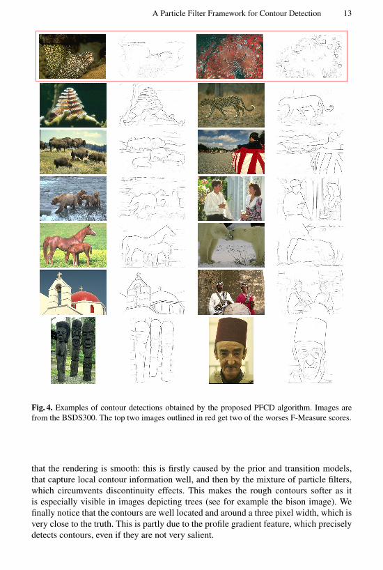
Fig. 4 illustrates a few contour detection results obtained by the proposed algorithm.The soft detection map is obtained using (15). By integrating the feature distributioninto the likelihood, the extracted information is adaptative to the image and enables tohighlight the most meaningful contours. Consequently, this removes noisy responsesand offers cleaner results. In particular, the skin texture is not detected in the imageof a leopard, since this information is not meaningful in the image. This behavior mayalso explain bad results observable in the first image (moray eel): the point of view istoo close, and the low amount of real contours are not salient enough to be relevant,this is why the data found in the texture is deemed meaningful. We can also observe


Fig. 4. Examples of contour detections obtained by the proposed PFCD algorithm. Images arefrom the BSDS300. The top two images outlined in red get two of the worses F-Measure scores.

that the rendering is smooth: this is firstly caused by the prior and transition models,that capture local contour information well, and then by the mixture of particle filters,which circumvents discontinuity effects. This makes the rough contours softer as itis especially visible in images depicting trees (see for example the bison image). Wefinally notice that the contours are well located and around a three pixel width, which isvery close to the truth. This is partly due to the profile gradient feature, which preciselydetects contours, even if they are not very salient.


5 Conclusion

We demonstrated throughout this paper the ability of the particle filter to track contoursin complex natural images. Its flexibility and genericity enable to embed semi-localprior and transition distributions learned on a shape database as well as adaptive like-lihoods that detect contextual relevant pieces of edge. Our contribution covers boththe learning stage and the tracking modeling. We tested our algorithm on the compet-ing BSDS300 [1] and BSDS500 [5] datasets, and obtained very promising results withF-Measure scores of 0.68 and 0.70, respectively. This might further be improved byintegrating multiscale features and global information.

References1. Martin, D., Fowlkes, C., Tal, D., Malik, J.: A Database of Human Segmented Natural Im-

ages and its Application to Evaluating Segmentation Algorithms and Measuring EcologicalStatistics. In: ICCV. Volume 2. (2001) 416–423

2. Martin, D., Fowlkes, C., Malik, J.: Learning to Detect Natural Image Boundaries UsingLocal Brightness, Color, and Texture Cues. PAMI 26 (2004) 530–549

3. Ren, X.: Multi-Scale Improves Boundary Detection in Natural Images. ICCV (2008) 533–545

4. Maire, M., Arbelaez, P., Fowlkes, C., Malik, J.: Using Contours to Detect and LocalizeJunctions in Natural Images. In: CVPR. (2008) 1–8

5. Arbelaez, P., Maire, M., Fowlkes, C., Malik, J.: Contour Detection and Hierarchical ImageSegmentation. PAMI 33 (2011) 898–916

6. Dollar, P., Tu, Z., Belongie, S.: Supervised Learning of Edges and Object Boundaries. In:CVPR. Volume 2. (2006) 1964–1971

7. Mairal, J., Leordeanu, M., Bach, F., Hebert, M., Ponce, J.: Discriminative Sparse ImageModels for Class-Specific Edge Detection and Image Interpretation. ECCV (2008) 43–56

8. Ren, X., Fowlkes, C., Malik, J.: Scale-Invariant Contour Completion using ConditionalRandom Fields. In: ICCV. Volume 2. (2005) 1214–1221

9. Felzenszwalb, P., McAllester, D.: A Min-Cover Approach for Finding Salient Curves. In:CVPRW. (2006) 185–185

10. Perez, P., Blake, A., Gangnet, M.: Jetstream: Probabilistic contour extraction with particles.In: ICCV. Volume 2. (2001) 524–531

11. Lu, C., Latecki, L., Zhu, G.: Contour Extraction using Particle Filters. Advances in VisualComputing (2008) 192–201

12. Korah, T., Rasmussen, C.: Probabilistic Contour Extraction with Model-Switching for Vehi-cle Localization. In: IEEE Intelligent Vehicles Symposium. (2004) 710–715

13. Pitie, F., Kokaram, A., Dahyot, R.: Oriented Particle Spray: Probabilistic Contour Tracingwith Directional Information. Irish Machine Vision and Image Processing (2004)

14. Desolneux, A., Moisan, L., Morel, J.: Edge detection by helmholtz principle. Journal ofMathematical Imaging and Vision 14 (2001) 271–284

15. Sun, J., Xu, Z., Shum, H.Y.: Gradient Profile Prior and Its Applications in Image Super-Resolution and Enhancement. IP 20 (2011) 1529–1542

16. Doucet, A., De Freitas, N., Gordon, N., eds.: Sequential Monte Carlo methods in practice.Springer (2001)

17. Chen, Z.: Bayesian filtering: From Kalman filters to particle filters, and beyond. Technicalreport, McMaster University (2003)

18. Catanzaro, B., Su, B., Sundaram, N., Lee, Y., Murphy, M., Keutzer, K.: Efficient, high-quality image contour detection. In: CVPR. (2009) 2381–2388

A Particle Filter Framework for Contour Detection

Documents

Transcript of A Particle Filter Framework for Contour Detection