A Paraperspective Factorization Method for Shape and Motion
36
School of Computer Science Carnegie Mellon University Pittsburgh, Pennsylvania 15213-3890 This report supersedes CMU-CS-92-208. Abstract The factorization method, first developed by Tomasi and Kanade, recovers both the shape of an object and its motion from a sequence of images, using many images and tracking many feature points to obtain highly redundant feature position information. The method robustly processes the feature trajec- tory information using singular value decomposition (SVD), taking advantage of the linear algebraic properties of orthographic projection. However, an orthographic formulation limits the range of motions the method can accommodate. Paraperspective projection, first introduced by Ohta, is a projection model that closely approximates perspective projection by modelling several effects not modelled under orthographic projection, while retaining linear algebraic properties. Our paraperspective factorization method can be applied to a much wider range of motion scenarios, such as image sequences containing significant translational motion toward the camera or across the image. The method also can accommo- date missing or uncertain tracking data, which occurs when feature points are occluded or leave the field of view. We present the results of several experiments which illustrate the method’s performance in a wide range of situations, including an aerial image sequence of terrain taken from a low-altitude air- plane. A Paraperspective Factorization Method for Shape and Motion Recovery Conrad J. Poelman and Takeo Kanade 11 December 1993 CMU-CS-93-219 This research was partially supported by the Avionics Laboratory, Wright Research and Development Center, Aero- nautical Systems Division (AFSC), U.S. Air Force, Wright-Patterson AFB, Ohio 45433-6543 under Contract F33615-90-C1465, ARPA Order No. 7597. The views and conclusions contained in this document are those of the authors and should not be interpreted as repre- senting the official policies, either expressed or implied, of the U.S. Air Force or the U.S. government.
Transcript of A Paraperspective Factorization Method for Shape and Motion
School of Computer ScienceCarnegie Mellon University
Pittsburgh, Pennsylvania 15213-3890
This report supersedes CMU-CS-92-208.
Abstract
The factorization method, first developed by Tomasi and Kanade, recovers both the shape of an objectand its motion from a sequence of images, using many images and tracking many feature points toobtain highly redundant feature position information. The method robustly processes the feature trajec-tory information using singular value decomposition (SVD), taking advantage of the linear algebraicproperties of orthographic projection. However, an orthographic formulation limits the range of motionsthe method can accommodate. Paraperspective projection, first introduced by Ohta, is a projectionmodel that closely approximates perspective projection by modelling several effects not modelled underorthographic projection, while retaining linear algebraic properties. Our paraperspective factorizationmethod can be applied to a much wider range of motion scenarios, such as image sequences containingsignificant translational motion toward the camera or across the image. The method also can accommo-date missing or uncertain tracking data, which occurs when feature points are occluded or leave the fieldof view. We present the results of several experiments which illustrate the method’s performance in awide range of situations, including an aerial image sequence of terrain taken from a low-altitude air-plane.
A Paraperspective Factorization Methodfor Shape and Motion Recovery
Conrad J. Poelman and Takeo Kanade
11 December 1993CMU-CS-93-219
This research was partially supported by the Avionics Laboratory, Wright Research and Development Center, Aero-nautical Systems Division (AFSC), U.S. Air Force, Wright-Patterson AFB, Ohio 45433-6543 under ContractF33615-90-C1465, ARPA Order No. 7597.
The views and conclusions contained in this document are those of the authors and should not be interpreted as repre-senting the official policies, either expressed or implied, of the U.S. Air Force or the U.S. government.

Keywords: computer vision, motion, shape, time-varying imagery, factorization method
page 3
1. Introduction
Recovering the geometry of a scene and the motion of the camera from a stream of images isan important task in a variety of applications, including navigation, robotic manipulation,and aerial cartography. While this is possible in principle, traditional methods have failed toproduce reliable results in many situations [2].
Tomasi and Kanade [10][11] developed a robust and efficient method for accurately recov-ering the shape and motion of an object from a sequence of images, called thefactorizationmethod. It achieves its accuracy and robustness by applying a well-understood numericalcomputation, the singular value decomposition (SVD), to a large number of images and fea-ture points, and by directly computing shape without computing the depth as an intermedi-ate step. The method was tested on a variety of real and synthetic images, and was shown toperform well even for distant objects.
The Tomasi-Kanade factorization method, however, assumed an orthographic projectionmodel, since it can be described by linear equations. The applicability of the method istherefore limited to image sequences created from certain types of camera motions. Theorthographic model contains no notion of the distance from the camera to the object. As aresult, shape reconstruction from image sequences containing large translations toward oraway from the camera often produces deformed object shapes, as the method tries to explainthe size differences in the images by creating size differences in the object. The method alsosupplies no estimation of translation along the camera’s optical axis, which limits its useful-ness for certain tasks.
There exist several perspective approximations which capture more of the effects of per-spective projection while remaining linear. Scaled orthographic projection, sometimesreferred to as “weak perspective” [4], accounts for the scaling effect of an object as it movestowards and away from the camera. Paraperspective projection, first introduced by Ohta [5]and named by Aloimonos [1], models the position effect (an object is viewed from differentangles as it translates across the field of view) as well as the scaling effect.
In this paper, we present a factorization method based on the paraperspective projectionmodel. The paraperspective factorization method is still fast, and robust with respect tonoise. It can be applied to a wider realm of situations than the original factorization method,such as sequences containing significant depth translation or containing objects close to thecamera, and can be used in applications where it is important to recover the distance to theobject in each image, such as navigation.
We begin by describing our camera and world reference frames and introduce the mathe-matical notation that we use. We review the original factorization method as defined in [11],presenting it in a slightly different manner in order to make its relation to the paraperspec-tive method more apparent. We then present our paraperspective factorization method, fol-lowed by an extension which accommodates occlusions. We conclude with the results ofseveral experiments which demonstrate the practicality of our system.

page 4
2. Problem Description
In a shape-from-motion problem, we are given a sequence of images taken from a camerathat is moving relative to an object. Assume for the time being that we locate prominentfeature points in the first image, and track these points from each image to the next, record-ing the coordinates of each point in each image . Each feature point that wetrack corresponds to a single world point, located at position in some fixed world coordi-nate system. Each image was taken at some camera orientation, which we describe by theorthonormal unit vectors , , and , where and correspond to the x and y axes of thecamera’s image plane, and points along the camera’s line of sight. We describe the posi-tion of the camera in each frame by the vector indicating the camera’s focal point. Thisformulation is illustrated in Figure 1.
The result of the feature tracker is a set of feature point coordinates for each ofthe frames of the image sequence. From this information, our goal is to estimate the shapeof the object as for each object point, and the motion of the camera as , , and foreach frame in the sequence.
In Section 6 we will relax the requirement that every feature point be visible in every frame,allowing the inclusion of feature points that are observed and tracked through only a portionof the sequence.
F
P
ufp vfp( , ) p f p
spf
i f j f k f i f j fk f
f t f
j f
k f
Figure 1. Coordinate system
worldorigin
t f sp
Camera
ImagePlane
focallengthl
i f
ufp vfp,
imaging ray
P ufp vfp( , )
F
sp i f j f k f t f
page 5
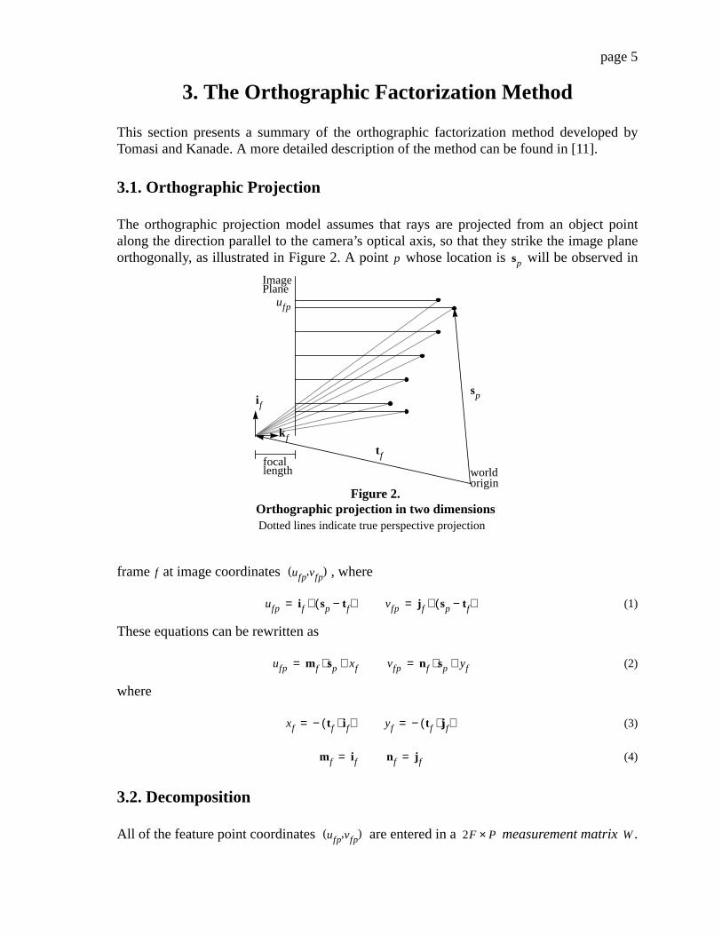
3. The Orthographic Factorization Method
This section presents a summary of the orthographic factorization method developed byTomasi and Kanade. A more detailed description of the method can be found in [11].
3.1. Orthographic Projection
The orthographic projection model assumes that rays are projected from an object pointalong the direction parallel to the camera’s optical axis, so that they strike the image planeorthogonally, as illustrated in Figure 2. A point whose location is will be observed in
frame at image coordinates , where
(1)
These equations can be rewritten as
(2)
where
(3)
(4)
3.2. Decomposition
All of the feature point coordinates are entered in a measurement matrix .
k f
i f
ImagePlane
Figure 2.Orthographic projection in two dimensions
sp
t ffocallength world
origin
Dotted lines indicate true perspective projection
ufp
p sp
f ufp vfp( , )
ufp i f sp t f−( )⋅= vfp j f sp t f−( )⋅=
ufp mf sp⋅ xf+= vfp nf sp⋅ yf+=
xf t f i f⋅( )−= yf t f j f⋅( )−=
mf i f= nf j f=
ufp vfp( , ) 2F P× W
page 6
(5)
Each column of the measurement matrix contains the observations for a single point, whileeach row contains the observed u-coordinates or v-coordinates for a single frame. Equation(2) for all points and frames can now be combined into the single matrix equation
, (6)
where is the motion matrix whose rows are the and vectors, is theshape matrix whose columns are the vectors, and is the translation vector whoseelements are the and .
Up to this point, Tomasi and Kanade placed no restrictions on the location of the world ori-gin, except that it be stationary with respect to the object. Without loss of generality, theyposition the world origin at the center of mass of the object, denoted by , so that
. (7)
Because the sum of any row of is zero, the sum of any row of is . This enablesthem to compute the element of the translation vector directly from , simply by aver-aging the row of the measurement matrix. The translation is the subtracted from , leav-ing a “registered” measurement matrix . Because is the product of a
motion matrix and a shape matrix , its rank is at most 3. When noise ispresent in the input, the will not be exactly of rank 3, so the Tomasi-Kanade factoriza-tion method uses the SVD to find the best rank 3 approximation to , factoring it into theproduct
. (8)
3.3. Normalization
The decomposition of equation (8) is only determined up to a linear transformation. Anynon-singular matrix and its inverse could be inserted between and , and theirproduct would still equal . Thus the actual motion and shape are given by
, (9)
with the appropriate invertible matrix selected. The correct can be determinedusing the fact that the rows of the motion matrix (which are the and vectors) repre-
W
u11 … u1P
… … …uF1 … uFP
v11 … v1P
… … …vF1 … vFP
=
W MS T 1 … 1+=
M 2F 3× mf nf S 3 P×sp T 2F 1×
xf yf
c
c1P
spp 1=
P
∑ 0= =
S i W PTiith T W
ith W
W* W T 1 … 1−= W*
2F 3× M 3 P× S
W*
W*
W* MS=
3 3× A M S
W*
M MA= S A 1− S=
3 3× A A
M mf nf
page 7
sent the camera axes, and therefore they must be of a certain form. Since and are unitvectors, we see from equation (4) that
, (10)
and because they are orthogonal,
. (11)
Equations (10) and (11) give us equations which we call themetric constraints. Usingthese constraints, we solve for the matrix which, when multiplied by , producesthe motion matrix that best satisfies these constraints. Once the matrix has been found,the shape and motion are computed from equation (9).
i f j f
mf2 1= nf
2 1=
mf nf⋅ 0=
3F
3 3× A M
M A
page 8
4. The Paraperspective Factorization Method
The Tomasi-Kanade factorization method was shown to be computationally inexpensiveand highly accurate, but its use of an orthographic projection assumption limited the meth-od’s applicability. For example, the method does not produce accurate results when there issignificant translation along the camera’s optical axis, because orthography does not accountfor the fact that an object appears larger when it is closer to the camera. We must model thisand other perspective effects in order to successfully recover shape and motion in a widerrange of situations. We choose an approximation to perspective projection known asparap-erspective projection, which was introduced by Ohta [5] in order to solve a shape from tex-ture problem. Although the paraperspective projection equations are more complex thanthose for orthography, their basic form is the same, enabling us develop a method analogousto that developed by Tomasi and Kanade.
4.1. Paraperspective Projection
Paraperspective projection closely approximates perspective projection by modelling boththe scaling effect (closer objects appear larger than distant ones) and the position effect(objects in the periphery of the image are viewed from a different angle than those near thecenter of projection [1]), while retaining the linear properties of orthographic projection.The paraperspective projection of an object onto an image, illustrated in Figure 3, involvestwo steps.
1. An object point is projected along the direction of the line connecting the focal pointof the camera to the object’s center of mass, onto a hypothetical image plane parallel tothe real image plane and passing through the object’s center of mass.
2. The point is then projected onto the real image plane using perspective projection.Because the hypothetical plane is parallel to the real image plane, this is equivalent tosimply scaling the point coordinates by the ratio of the camera focal length and the dis-tance between the two planes.1
In general, the projection of a point along direction , onto the plane defined by its normal and distance from the origin , is given by the equation
. (12)
In frame , each object point is projected along the direction (which is the directionfrom the camera’s focal point to the object’s center of mass) onto the plane defined by nor-mal and distance from the origin . The result of this projection is
1. The scaled orthographic projection model (also known as “weak perspective”) is similar to paraperspective projection,except that the direction of the initial projection in step 1 is parallel to the camera’s optical axis rather than parallel to theline connecting the object’s center of mass to the camera’s focal point. This model captures the scaling effect of perspectiveprojection, but not the position effect. (See Appendix I.)
p rn d
p' pp n⋅ d−
r n⋅r−=
f sp c tf−
k f c kf⋅ s' fp
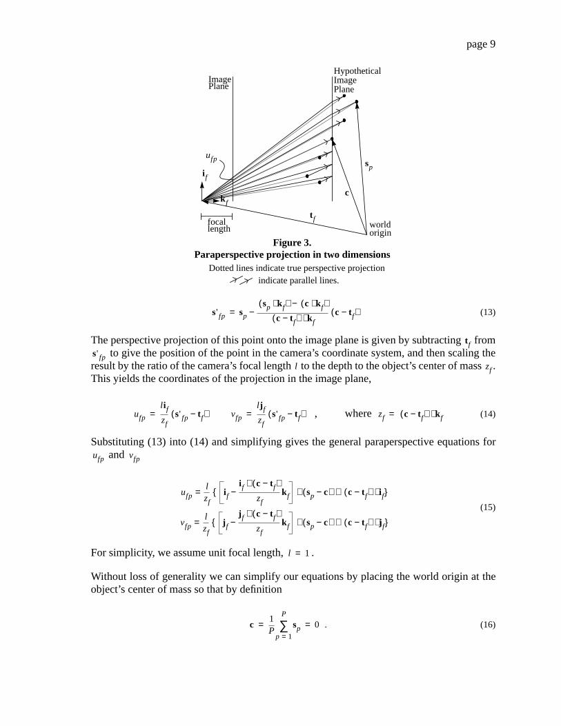
page 9
(13)
The perspective projection of this point onto the image plane is given by subtracting from to give the position of the point in the camera’s coordinate system, and then scaling the
result by the ratio of the camera’s focal length to the depth to the object’s center of mass .This yields the coordinates of the projection in the image plane,
, where (14)
Substituting (13) into (14) and simplifying gives the general paraperspective equations for and
(15)
For simplicity, we assume unit focal length, .
Without loss of generality we can simplify our equations by placing the world origin at theobject’s center of mass so that by definition
. (16)
k f
i f
ImagePlane
Figure 3.Paraperspective projection in two dimensions
c
t ffocallength world
origin
Dotted lines indicate true perspective projectionindicate parallel lines.
ufp sp
HypotheticalImagePlane
s' fp sp
sp k f⋅( ) c kf⋅( )−c tf−( ) k f⋅
c tf−( )−=
t fs' fp
l zf
ufp
l i fzf
s' fp t f−( )= vfp
l j f
zfs' fp t f−( )= zf c tf−( ) k f⋅=
ufp vfp
ufplzf
i fi f c tf−( )⋅
zfk f− sp c−( ) c tf−( ) i f⋅+⋅{ }=
vfplzf
j f
j f c tf−( )⋅zf
k f− sp c−( ) c tf−( ) j f⋅+⋅{ }=
l 1=
c1P
spp 1=
P
∑ 0= =

page 10
This reduces (15) to
(17)
These equations can be rewritten as
(18)
where
(19)
(20)
(21)
Notice that equation (18) has a form identical to its counterpart for orthographic projection,equation (2), although the corresponding definitions of , , , and differ. This enablesus to perform the basic decomposition of the matrix in the same manner that Tomasi andKanade did for the orthographic case.
4.2. Paraperspective Decomposition
We can combine equation (18), for all points from to , and all frames from to ,into the single matrix equation
, (22)
or in short
, (23)
where is the measurement matrix, is the motion matrix, is theshape matrix, and is the translation vector.
ufp1zf
i fi f t f⋅
zfk f+ sp t f i f⋅( )−⋅{ }=
vfp1zf
j f
j f t f⋅zf
k f+ sp t f j f⋅( )−⋅{ }=
ufp mf sp⋅ xf+= vfp nf sp⋅ yf+=
zf t− f k f⋅=
xf
t f i f⋅zf
−= yf
t f j f⋅zf
−=
mf
i f xfk f−zf
= nf
j f yfk f−zf
=
xf yf mf nf
p 1 P f 1 F
u11 … u1P
… … …uF1 … uFP
v11 … v1P
… … …vF1 … vFP
m1
…mF
n1
…nF
s1 … sP
x1
…xF
y1
…yF
1 … 1+=
W MS T 1 … 1+=
W 2F P× M 2F 3× S 3 P×T 2F 1×

page 11
Using equations (16) and (18) we can write
(24)
Therefore we can compute and , which are the elements of the translation vector ,immediately from the image data as
. (25)
Once we know the translation vector , we subtract it from , giving the registered mea-surement matrix
. (26)
Since is the product of two matrices each of rank at most 3, has rank at most 3, justas it did in the orthographic projection case. When noise is present, the rank of will notbe exactly 3, but by computing the SVD of and only retaining the largest 3 singular val-ues, we can factor it into
, (27)
where is a matrix and is a matrix. Using the SVD to perform this factor-ization guarantees that the product is the best possible rank 3 approximation to , inthe sense that it minimizes the sum of squares difference between corresponding elements of
and .
4.3. Paraperspective Normalization
Just as in the orthographic case, the decomposition of into the product of and byequation (27) is only determined up to a linear transformation matrix . Again, we deter-mine this matrix by observing that the rows of the motion matrix (the and vec-tors) must be of a certain form. Taking advantage of the fact that , , and are unitvectors, from equation (21) we observe that
. (28)
We know the values of and from our initial registration step, but we do not know thevalue of the depth . Thus we cannot impose individual constraints on the magnitudes ofand as was done in the orthographic factorization method. Instead we adopt the followingconstraint on the magnitudes of and
ufpp 1=
P
∑ mf sp⋅ xf+( )p 1=
P
∑ mf spp 1=
P
∑⋅ Pxf+ Pxf= = =
vfpp 1=
P
∑ nf sp⋅ yf+( )p 1=
P
∑ nf spp 1=
P
∑⋅ Pyf+ Pyf= = =
xf yf T
xf1P
ufpp 1=
P
∑= yf1P
vfpp 1=
P
∑=
T W
W* W T 1 … 1− MS= =
W* W*
W*
W*
W* MS=
M 2F 3× S 3 P×MS W*
W* MS
W* M S
A
A M mf nfi f j f k f
mf2
1 xf2+
zf2
= nf2
1 yf2+
zf2
=
xf yfzf mf
nfmf nf

page 12
. (29)
In the case of orthographic projection, one constraint on and was that they each haveunit magnitude, as required by equation (10). In the above paraperspective case, we simplyrequire that their magnitudes be in a certain ratio.
There is also a constraint on the angle relationship of and . From equation (21), and theknowledge that , , and are orthogonal unit vectors,
. (30)
The problem with this constraint is that, again, is unknown. We could use either of thetwo values given in equation (29) for , but in the presence of noisy input data the twowill not be exactly equal, so we use the average of the two quantities. We choose the arith-metic mean over the geometric mean or some other measure in order to keep the solution ofthese constraints linear. Thus our second constraint becomes
. (31)
This is the paraperspective version of the orthographic constraint given by equation (11),which required that the dot product of and be zero.
Equations (29) and (31) are homogeneous constraints, which could be trivially satisfied bythe solution , or . To avoid this solution, we impose the additionalconstraint
. (32)
This does not effect the final solution except by a scaling factor.
Equations (29), (31), and (32) gives us equations, which are the paraperspective ver-sion of themetric constraints. We compute the matrix such that best satis-fies these metric constraints in the least sum-of-squares error sense. This is a simple problembecause the constraints are linear in the 6 unique elements of the symmetric matrix
. We use the metric constraints to compute , compute its Jacobi Transformation, where is the diagonal eigenvalue matrix, and as long as is positive definite,
.
4.4. Paraperspective Motion Recovery
Once the matrix has been determined, we compute the shape matrix and themotion matrix . For each frame , we now need to recover the camera orientation
mf2
1 xf2+
nf2
1 yf2+
= 1
zf2
=
mf nf
mf nfi f j f k f
mf nf⋅i f xfk f−
zf
j f yfk f−zf
⋅xfyf
zf2
= =
zf1 zf
2⁄
mf nf⋅ xfyf12
mf2
1 xf2+
nf2
1 yf2+
+ =
mf nf
f mf∀ nf 0= = M 0=
m1 1=
2F 1+3 3× A M MA=
3 3×Q ATA= Q
Q LΛLT= Λ Q
A LΛ1 2⁄( )T
=
A S A 1− S=M MA= f
page 13
vectors , , and from the vectors and , which are the rows of the matrix . Fromequation (21) we see that
. (33)
From this and the knowledge that , , and must be orthonormal, we determine that
(34)
Again, we do not know a value for , but using the relations specified in equation (29) andthe additional knowledge that , equation (34) can be reduced to
, (35)
where
(36)
(37)
We compute simply as
(38)
and then compute
. (39)
There is no guarantee that the and given by this equation will be orthonormal, because and may not have exactly satisfied the metric constraints. Therefore we actually use
the orthonormals which are closest to the and vectors given by equation (39). Due to thearbitrary world coordinate orientation, to obtain a unique solution we then rotate the com-puted shape and motion to align the world axes with the first frame’s camera axes, so that
and .
All that remain to be computed are the translations for each frame. We calculate the depthfrom equation (29). Since we know , , , , , and , we can calculate using equa-tions (19) and (20).
i f j f k f mf nf M
i f zfmf xfk f+= j f zfnf yfk f+=
i f j f k f
i f j f× zfmf xfk f+( ) zfnf yfk f+( )× k f= =
i f zfmf xfk f+ 1= =
j f zfnf yfk f+ 1= =
zfk f 1=
Gfk f Hf=
Gf
mf nf×( )
mf
nf
= Hf
1
xf−
yf−=
mf 1 xf2+
mf
mf= nf 1 yf
2+nf
nf=
k f
k f Gf1− Hf=
i f nf k f×= j f k f mf×=
i f j f
mf nfi f j f
i1 1 0 0T
= j 1 0 1 0T
=
zfxf yf zf i f j f k f t f
page 14
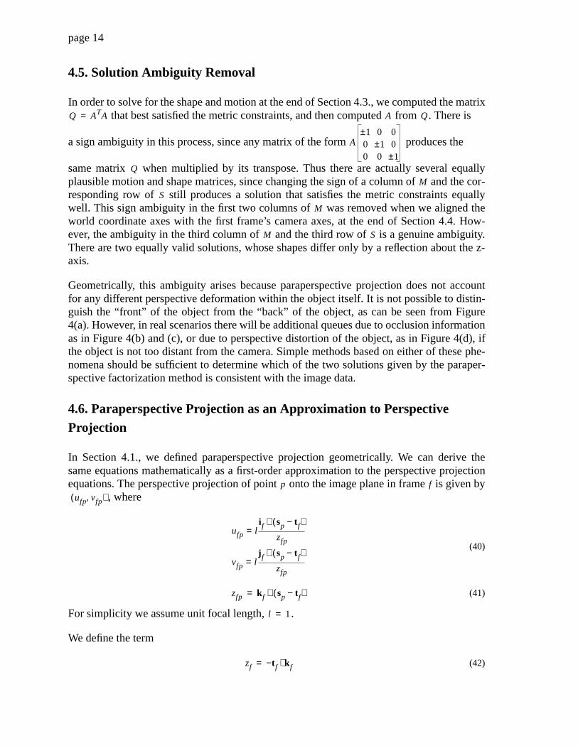
4.5. Solution Ambiguity Removal
In order to solve for the shape and motion at the end of Section 4.3., we computed the matrix that best satisfied the metric constraints, and then computed from . There is
a sign ambiguity in this process, since any matrix of the form produces the
same matrix when multiplied by its transpose. Thus there are actually several equallyplausible motion and shape matrices, since changing the sign of a column of and the cor-responding row of still produces a solution that satisfies the metric constraints equallywell. This sign ambiguity in the first two columns of was removed when we aligned theworld coordinate axes with the first frame’s camera axes, at the end of Section 4.4. How-ever, the ambiguity in the third column of and the third row of is a genuine ambiguity.There are two equally valid solutions, whose shapes differ only by a reflection about the z-axis.
Geometrically, this ambiguity arises because paraperspective projection does not accountfor any different perspective deformation within the object itself. It is not possible to distin-guish the “front” of the object from the “back” of the object, as can be seen from Figure4(a). However, in real scenarios there will be additional queues due to occlusion informationas in Figure 4(b) and (c), or due to perspective distortion of the object, as in Figure 4(d), ifthe object is not too distant from the camera. Simple methods based on either of these phe-nomena should be sufficient to determine which of the two solutions given by the paraper-spective factorization method is consistent with the image data.
4.6. Paraperspective Projection as an Approximation to PerspectiveProjection
In Section 4.1., we defined paraperspective projection geometrically. We can derive thesame equations mathematically as a first-order approximation to the perspective projectionequations. The perspective projection of point onto the image plane in frame is given by
, where
(40)
(41)
For simplicity we assume unit focal length, .
We define the term
(42)
Q ATA= A Q
A1± 0 0
0 1± 00 0 1±
Q
M
S
M
M S
p f
ufp vfp,( )
ufp li f sp t f−( )⋅
zfp=
vfp lj f sp t f−( )⋅
zfp=
zfp k f sp t f−( )⋅=
l 1=
zf t− f k f⋅=

page 15
and then compute the Taylor series expansion of the above equations about the point
(43)
yielding
(44)
We combine equations (41) and (42) to determine that , and substitute thisinto equation (44) to produce
(45)
Ignoring all but the first term of the Taylor series yields the equations for scaled orthogra-phic projection (See Appendix I.) However, instead of arbitrarily stopping at the first term,
(b) (c) (d)(a)
Figure 4 Ambiguity of Solution(a) Sequence of images with two valid motion and shape interpretations.(b), (c) Ambiguity removed due to occlusion information in the image sequence.(d) Ambiguity removed due to perspective distortion of the object in the images
Frame 1
Frame 2
Frame 3
Frame 4
zfp zf≈
ufp
i f sp t f−( )⋅zf
i f sp t f−( )⋅
zf2
zfp zf−( )− 12
i f sp t f−( )⋅
zf3
zfp zf−( ) 2 …+ +=
vfp
j f sp t f−( )⋅zf
j f sp t f−( )⋅
zf2
zfp zf−( )− 12
j f sp t f−( )⋅
zf3
zfp zf−( ) 2 …+ +=
zfp zf− k f sp⋅=
ufp
i f sp t f−( )⋅zf
i f sp t f−( )⋅
zf2
k f sp⋅( )− 12
i f sp t f−( )⋅
zf3
k f sp⋅( ) 2 …+ +=
vfp
j f sp t f−( )⋅zf
j f sp t f−( )⋅
zf2
k f sp⋅( )− 12
j f sp t f−( )⋅
zf3
k f sp⋅( ) 2 …+ +=
page 16
we eliminate higher order terms based on the approximation that , which will beaccurate when the size of the object is smaller than the distance of the object from the cam-era. Eliminating these terms reduces the equation (45) to
(46)
Factoring out the and expanding the dot-products and gives
(47)
These equations are equivalent to the paraperspective projection equations given by equa-tion (17).
The approximation that preserves the portion of the second term of the Taylorseries expansion of order , while ignoring the portion of the second term of order
and all higher order terms. Clearly if the translation that the object undergoes is alsosmall, then there is little justification for preserving this portion of the second term and notthe other. In such cases, the entire second term can be safely ignored, leaving only the equa-tions for scaled orthographic projection.
Note that we did not explicitly set the world origin at the object’s center of mass, as we didin Section 4.1. However, the assumption that will be most accurate when themagnitudes of the are smallest. Since the vectors represent the vectors from the worldorigin to the object points, their magnitudes will be smaller when the world origin is locatednear the object’s center of mass.
sp2 zf
2⁄ 0=
ufp
i f sp t f−( )⋅zf
i f t f−( )⋅
zf2
k f sp⋅( )−=
vfp
j f sp t f−( )⋅zf
j f t f−( )⋅
zf2
k f sp⋅( )−=
1 zf⁄ i f sp t f−( )⋅ j f sp t f−( )⋅
ufp1zf
i f sp⋅i f t f⋅
zfk f sp⋅( ) i f t f⋅( )−+
=
vfp1zf
j f sp⋅j f t f⋅
zfk f sp⋅( ) j f t f⋅( )−+
=
sp2 zf
2⁄ 0=sp t f( ) zf
2⁄sp
2 zf2⁄
sp2 zf
2⁄ 0=sp sp
page 17
5. Comparison of Methods using Synthetic Data
In this section we compare the performance of our new paraperspective factorizationmethod with the previous orthographic factorization method. The comparison also includesa factorization method based on scaled orthographic projection (also known as “weak per-spective”), which models the scaling effect of perspective projection but not the positioneffect, in order to demonstrate the importance of modelling the position effect for objects atclose range. (See Appendix I.) Our results show that the paraperspective factorizationmethod is a vast improvement over the orthographic method, and underscore the importanceof modelling both the scaling and position effects.
5.1. Data Generation
The synthetic feature point sequences used for comparison were created by moving a known“object” - a set of 3D points - through a known motion sequence. We tested three differentobject shapes, each containing approximately 60 points. Each test run consisted of 60 imageframes of an object rotating through a total of 30 degrees each of roll, pitch, and yaw. The“object depth” - the distance from the camera’s focal point to the front of the object - in thefirst frame was varied from 3 to 60 times the object size. In each sequence, the object trans-lated across the field of view by a distance of one object size horizontally and vertically, andtranslated away from the camera by half its initial distance from the camera. For example,when the object’s depth in the first frame was 3.0, its depth in the last frame was 4.5. Each“image” was created by perspectively projecting the 3D points onto the image plane, foreach sequence choosing the largest focal length that would keep the object in the field ofview throughout the sequence. The coordinates in the image plane were perturbed by addinggaussian noise, to model tracking imprecision. The standard deviation of the noise was 2pixels (assuming a 512x512 pixel image), which we consider to be a rather high noise levelfrom our experience processing real image sequences. For each combination of object,depth, and noise, we performed three tests, using different random noise each time.
5.2. Error Measurement
We ran each of the three factorization methods on each synthetic sequence and measured therotation error, shape error, X-Y offset error, and Z offset (depth) error. The rotation error isthe root-mean-square (RMS) of the size in radians of the angle by which the computed cam-era coordinate frame must be rotated about some axis to produce the known camera orienta-tion. The shape error is the RMS error between the known and computed 3D pointcoordinates. Since the shape and translations are only determined up to scaling factor, wefirst scaled the computed shape by the factor which minimizes this RMS error. The term“offset” refers to the translational component of the motion as measured in the camera’scoordinate frame rather than in world coordinates; the X offset is , the Y offset is ,and the Z offset is . The X-Y offset error and Z offset error are the RMS error betweenthe known and computed offset; like the shape error, we first scaled the computed offset bythe scale factor that minimized the RMS error. Note that the orthographic factorization
t f i f⋅ t f j f⋅t f k f⋅
page 18
method supplies no estimation of translation along the camera’s optical axis, so the Z offseterror cannot be computed for that method.
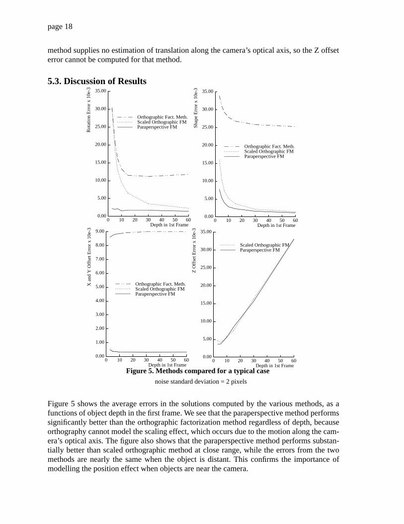
5.3. Discussion of Results
Figure 5 shows the average errors in the solutions computed by the various methods, as afunctions of object depth in the first frame. We see that the paraperspective method performssignificantly better than the orthographic factorization method regardless of depth, becauseorthography cannot model the scaling effect, which occurs due to the motion along the cam-era’s optical axis. The figure also shows that the paraperspective method performs substan-tially better than scaled orthographic method at close range, while the errors from the twomethods are nearly the same when the object is distant. This confirms the importance ofmodelling the position effect when objects are near the camera.
0.00
5.00
10.00
15.00
20.00
25.00
30.00
35.00R
otat
ion
Err
or x
10e
-3
0 10 20 30 40 50 60Depth in 1st Frame
Paraperspective FMScaled Orthographic FMOrthographic Fact. Meth.
0.00
5.00
10.00
15.00
20.00
25.00
30.00
35.00
Shap
e E
rror
x 1
0e-3
0 10 20 30 40 50 60Depth in 1st Frame
Paraperspective FMScaled Orthographic FMOrthographic Fact. Meth.
0.00
1.00
2.00
3.00
4.00
5.00
6.00
7.00
8.00
9.00
X a
nd Y
Off
set E
rror
x 1
0e-3
0 10 20 30 40 50 60Depth in 1st Frame
Paraperspective FMScaled Orthographic FMOrthographic Fact. Meth.
0.00
5.00
10.00
15.00
20.00
25.00
30.00
35.00
Z O
ffse
t Err
or x
10e
-3
0 10 20 30 40 50 60Depth in 1st Frame
Paraperspective FMScaled Orthographic FM
Figure 5. Methods compared for a typical casenoise standard deviation = 2 pixels
page 19
In other experiments in which the object was centered in the image and there was no transla-tion across the field of view, the paraperspective method and the scaled orthographic methodperformed equally well, as we would expect since such image sequences contain no positioneffects. Similarly, we found that when the object remained centered in the image and therewas no depth translation, the orthographic factorization method performed very well, andthe paraperspective factorization method provided no significant improvement since suchsequences contain neither scaling effects nor position effects.
To examine the impact of those effects of perspective projection which are not modelled byparaperspective projection, we implemented an iterative method which refines the results ofthe paraperspective method using a perspective projection model. (See Appendix II.) Com-puting this refined solution required more than ten times as long as computing the initialparaperspective results. We tested the method on the same sequences that were tested to pro-duce Figure 5, and found the resulting shape and motion errors to be nearly invariant todepth. The perspective refinement method only minimally improved the motion results overthe paraperspective solution. However, the shape results were significantly improved forthose cases in which the depth was less than 30. This implies that unmodelled perspectivedistortion in the images effects primarily the shape portion of the paraperspective factoriza-tion method’s solution, and that the effects are significant only when the object is within acertain distance of the camera.
5.4. Analysis of Paraperspective Method using Synthetic Data
Now that we have shown the advantages of the paraperspective factorization method overthe previous method, we further analyze the performance of the paraperspective method todetermine its behavior at various depths and its robustness with respect to noise. The syn-thetic sequences used in these experiments were created in the same manner as in the previ-ous section, except that the standard deviation of the noise was varied from 0 to 4.0 pixels.
In Figure 6, we see that at high depth values, the error in the solution is roughly proportionalto the level of noise in the input, while at low depths the error is inversely related to thedepth. This occurs because at low depths, perspective distortion of the object’s shape is theprimary source of error in the computed results. At higher depths, perspective distortion ofthe object’s shape is negligible, and noise becomes the dominant cause of error in theresults. For example, at a noise level of 1 pixel, the rotation and XY-offset errors are nearlyinvariant to the depth once the object is farther from the camera than 10 times the objectsize. The shape results, however, appear sensitive to perspective distortion even at depths of30 or 60 times the object size.

page 20
0.00
10.00
20.00
30.00
40.00
50.00
60.00
70.00Z
Off
set E
rror
x 1
0e-3
0 10 20 30 40 50 60Depth in 1st Frame
Noise sigma=0 pixelsNoise sigma=0.5 pixelsNoise sigma=1 pixelsNoise sigma=1.5 pixelsNoise sigma=2 pixelsNoise sigma=3 pixelsNoise sigma=4 pixels
0.00
100.00
200.00
300.00
400.00
500.00
600.00
700.00
800.00
X a
nd Y
Off
set E
rror
x 1
0e-6
0 10 20 30 40 50 60Depth in 1st Frame
Noise sigma=0 pixelsNoise sigma=0.5 pixelsNoise sigma=1 pixelsNoise sigma=1.5 pixelsNoise sigma=2 pixelsNoise sigma=3 pixelsNoise sigma=4 pixels
0.00
0.50
1.00
1.50
2.00
2.50
3.00
3.50
4.00
Rot
atio
n E
rror
x 1
0e-3
0 10 20 30 40 50 60Depth in 1st Frame
Noise sigma=0 pixelsNoise sigma=0.5 pixelsNoise sigma=1 pixelsNoise sigma=1.5 pixelsNoise sigma=2 pixelsNoise sigma=3 pixelsNoise sigma=4 pixels
0.00
1.00
2.00
3.00
4.00
5.00
6.00
7.00
8.00
Shap
e E
rror
x 1
0e-3
0 10 20 30 40 50 60Depth in 1st Frame
Noise sigma=0 pixelsNoise sigma=0.5 pixelsNoise sigma=1 pixelsNoise sigma=1.5 pixelsNoise sigma=2 pixelsNoise sigma=3 pixelsNoise sigma=4 pixels
Figure 6. Paraperspective shape and motionrecovery by noise level

page 21
6. Accommodating Occlusion andUncertain Tracking Data
So far, we have assumed that all of the entries of the measurement matrix are known and areequally reliable. In real image sequences, this is not the case. Some feature points are nottracked throughout the entire sequence because they leave the field of view, becomeoccluded, or change their appearance significantly enough that the feature tracker can nolonger track them. As the object moves, new feature points can be detected on parts of theobject which were not visible in the initial image. Thus the measurement matrix is notentirely filled; there are some pairs for which was not observed.
Not all observed position measurements are known with the same confidence. Some featurewindows contain sharp, trackable features, enabling exact localization, while others mayhave significantly less texture information. Some matchings are very exact, while others areless exact due to unmodelled change in the appearance of a feature. Previously, using somearbitrary criteria, each measurement was either accepted or rejected as too unreliable, andthen all accepted observations were treated equally throughout the method.
We address both of these issues by assigning a confidence value to each measurement, andmodifying our method to weight each measurement by its corresponding confidence value.If a feature is not observed in some frames, the confidence values corresponding to thosemeasurements are set to zero.
6.1. Confidence-Weighted Formulation and Solution Method
We can view the decomposition step of Section 4.2. as a way, given the measurement matrix, to compute an , , and that satisfy the equation
(48)
There, our first step was to compute directly from . We then used the SVD to factor thematrix into the product of and . In fact, using the SVD to performthis factorization produced an and that, given and the just computed from , min-imized the error
(49)
In our new confidence-weighted formulation, we associate each element of the measure-ment matrix with a confidence value . We incorporate these confidences into thefactorization method by reformulating the decomposition step as a weighted least squaresproblem, in which we seek the , , and which minimize the error
W
f p,( ) ufp vfp( , )
W M S T
W MS T 1 … 1+=
T W
W* W T 1 … 1−= M S
M S W T W
ε0 Wrp Mr1S1p Mr2S2p Mr3S3p Tr+ + +( )−( )p 1=
P
∑2
r 1=
2F
∑=
Wrp γrp
M S T

page 22
(50)
Once we have solved this minimization problem for , , and , we can proceed with thenormalization step and the rest of the shape and motion recovery process precisely asbefore.
There is sufficient mathematical constraint to compute , , and , provided the number ofknown elements of exceeds the total number of variables ( ). The minimization ofequation (50) is a nonlinear least squares problem because each term contains products ofthe variables and . However, it is separable; the set of variables can be partitionedinto two subsets, the motion variables and the shape variables, so that the problem becomesa simple linear least squares problem with respect to one subset when the other is known.We use a variant of an algorithm suggested by Ruhe and Wedin [8] for solving such prob-lems - one that is equivalent to alternately refining the two sets of variables. In other words,we hold fixed at some value and solve for the and which minimize . Then holding
and fixed, we solve for the which minimizes . Each step of the iteration is simpleand fast since, as we will show shortly, it is a series of linear least squares problems. Werepeat the process until a step of the iteration produces no significant reduction in the error
.
To compute and for a given , we first rewrite the minimization of equation (50) as
, where . (51)
For a fixed , the total error can be minimized by independently minimizing each error ,since no variable appears in more than one equation. Each describes a weighted linearleast squares problem in the variables , , , and . For every row , the fourvariables are computed by finding the least squares solution to the overconstrained linearsystem of variables and equations
(52)
Similarly, for a fixed and , each column of can be computed independently of theother columns, by finding the least squares solution to the linear system of variables and
equations
ε γ2rp Wrp Mr1S1p Mr2S2p Mr3S3p Tr+ + +( )−( )
2
p 1=
P
∑r 1=
2F
∑=
M S T
M S T
W 8F 3P+
Mrj Sjp
S M T εM T S ε
ε
M T S
ε εrr 1=
2F
∑= εr γ2rp Wrp Mr1S1p Mr2S2p Mr3S3p Tr+ + +( )−( )
2
p 1=
P
∑=
S ε εrεr εr
Mr1 Mr2 Mr3 Tr r
4 P
S11γr1 S21γr1 S31γr1 γr1
… … … …
S1PγrP S2PγrP S3PγrP γrP
Mr1
Mr2
Mr3
Tr
Wr1γr1
…WrPγrP
=
M T pth S
3
2F

page 23
(53)
As in any iterative method, an initial value is needed to begin the process. Our initial exper-iments showed, however, that when the confidence matrix contained few zero values, themethod consistently converged to the correct solution in a small number of iterations, evenbeginning with a random initial value. For example, in the special case of (whichcorresponds to the case in which all features are tracked throughout the entire sequence andare known with equal confidence), the method always converged in 5 or fewer iterations,requiring even less time than computing the singular value decomposition of ; when the
were randomly given values ranging from 1 to 10, the method generally converged in 10or fewer iterations; and with a whose fill fraction (fraction of non-zero entries) was 0.8,the method converged in 20 or fewer iterations. However, when the fill fraction decreased to0.6, the method sometimes failed to converge even after 100 iterations.
In order to apply the method to sequences with lower fill fractions, it is critical that weobtain a reasonable initial value before proceeding with the iteration. We developed anapproach analogous to the propagation method described in [11]. We first find a subset ofrows and columns of for which all of the confidences are non-zero, and solve for the cor-responding rows of and and columns of by running the iterative method starting witha random initial value. As indicated above, this converges quickly, producing estimated val-ues for this subset of , , and . We can solve for one additional row of and by solv-ing the linear least squares problem of equation (52) using only the known columns of .We can solve for one additional column of by solving the linear least squares problem ofequation (53) using only the known rows of and . We continue solving for additionalrows of and or columns of until , , and are completely known. Using this as theinitial value allows the iterative method to converge in far fewer iterations.
6.2. Analysis of Weighted Factorization using Synthetic Data
We tested the confidence-weighted paraperspective factorization method with artificiallygenerated measurement matrices and confidence matrices whose fill fraction (fraction ofnon-zero entries) was varied from 1.0 down to 0.21. Figure 7 shows how the performancedegrades as the noise level increases and fill fraction decreases. The synthetic sequenceswere of a single object consisting of 99 points, initially located 60 times the object size fromthe camera. Each data point represents the average solution error over 5 runs, using a differ-ent seed for the random noise. The motion, method of generating the sequences, and errormeasures are as described in Section 5.
Errors in the recovered motion only increase slightly as the fill fraction decreases from 1.0
1. Creating a confidence matrix that has a given fill fraction and a fairly realistic fill pattern (the arrangement of zero andnon-zero entries in the matrix) is a non-trivial task. We first create the synthetic feature tracks resulting from the givenobject and motion, by detecting when points become occluded by some surface of the object. These feature tracks are thenextended or shortened until the desired fill fraction is achieved.
M11γ1p M12γ1p M13γ1p
… … …
M2F 1, γ2F p, M2F 2, γ2F p, M2F 3, γ2F p,
S1p
S2p
S3p
W1p T1−( ) γ1p
…W2F p, T2F−( ) γ2F p,
=
γrp 1.0=
W
γrpγ
W
M T S
M S T M T
S
S
M T
M T S M S T

page 24
to 0.5. At a very low noise level, such as 0.1 pixels, this behavior continues down to a fillfraction of 0.3. When the fill fraction is decreased below this range, however, the error in therecovered motion increases very sharply. The shape results appear more sensitive todecreased fill fractions; as the fill fraction drops to 0.8 or lower, the shape error increasessharply, and then increases dramatically when the fill fraction reaches 0.6 or 0.5. While thesystem of equations defined by equation (50) is still overconstrained at these lower fill frac-tions, apparently there is insufficient redundancy to overcome the effects of the noise in thedata.
0.00
2.00
4.00
6.00
8.00
10.00
12.00
14.00
16.00
18.00
20.00
Rot
atio
n E
rror
x 1
0e-3
0.2 0.3 0.4 0.5 0.6 0.7 0.8 0.9 1.0Fill Fraction
Figure 7. Confidence-Weighted Shape andMotion Recovery by Noise Level, Fill Fraction
0.00
1.00
2.00
3.00
4.00
5.00
6.00
7.00
8.00
9.00
10.00
Shap
e E
rror
x 1
0e-3
0.2 0.3 0.4 0.5 0.6 0.7 0.8 0.9 1.0Fill Fraction
0.00
1.00
2.00
3.00
4.00
5.00
6.00
7.00
8.00
9.00
10.00
X a
nd Y
Off
set E
rror
x 1
0e-3
0.2 0.3 0.4 0.5 0.6 0.7 0.8 0.9 1.0Fill Fraction
Noise sigma=0 pixelsNoise sigma=0.1 pixelsNoise sigma=0.5 pixelsNoise sigma=1 pixelsNoise sigma=1.5 pixelsNoise sigma=2 pixels
0.00
0.02
0.04
0.06
0.08
0.10
0.12
0.14
0.16
0.18
0.20
Z O
ffse
t Err
or
0.2 0.3 0.4 0.5 0.6 0.7 0.8 0.9 1.0Fill Fraction

page 25
7. Shape and Motion Recovery fromReal Image Sequences
We tested the paraperspective factorization method on two real image sequences - a labora-tory experiment in which a small model building was imaged, and an aerial sequence takenfrom a low-altitude plane using a hand-held video camera. Both sequences contain signifi-cant perspective effects, due to translations along the optical axis and across the field ofview. We implemented a system to automatically identify and track features, based on[11] and [3]. This tracker computes the position of a square feature window by minimizingthe sum of the squares of the intensity difference over the feature window from one image tothe next.
7.1. Hotel Model Sequence
A hotel model was imaged by a camera mounted on a computer-controlled movable plat-form. The camera motion included substantial translation away from the camera and acrossthe field of view (see Figure 8). The feature tracker automatically identified and tracked 197points throughout the sequence of 181 images.
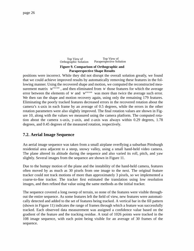
Both the paraperspective factorization method and the orthographic factorization methodwere tested with this sequence. The shape recovered by the orthographic factorizationmethod was rather deformed (see Figure 9) and the recovered motion incorrect, because themethod could not account for the scaling and position effects which are prominent in thesequence. The paraperspective factorization method, however, models these effects of per-spective projection, and therefore produced an accurate shape and accurate motion.
Several features in the sequence were poorly tracked, and as a result their recovered 3D
Frame 1
Frame 151Frame 121
Frame 61
Figure 8. Hotel Model Image Sequence
page 26
positions were incorrect. While they did not disrupt the overall solution greatly, we foundthat we could achieve improved results by automatically removing these features in the fol-lowing manner. Using the recovered shape and motion, we computed the reconstructed mea-surement matrix , and then eliminated from those features for which the averageerror between the elements of and was more than twice the average such error.We then ran the shape and motion recovery again, using only the remaining 179 features.Eliminating the poorly tracked features decreased errors in the recovered rotation about thecamera’s x-axis in each frame by an average of 0.5 degrees, while the errors in the otherrotation parameters were also slightly improved. The final rotation values are shown in Fig-ure 10, along with the values we measured using the camera platform. The computed rota-tion about the camera x-axis, y-axis, and z-axis was always within 0.29 degrees, 1.78degrees, and 0.45 degrees of the measured rotation, respectively.
7.2. Aerial Image Sequence
An aerial image sequence was taken from a small airplane overflying a suburban Pittsburghresidential area adjacent to a steep, snowy valley, using a small hand-held video camera.The plane altered its altitude during the sequence and also varied its roll, pitch, and yawslightly. Several images from the sequence are shown in Figure 11.
Due to the bumpy motion of the plane and the instability of the hand-held camera, featuresoften moved by as much as 30 pixels from one image to the next. The original featuretracker could not track motions of more than approximately 3 pixels, so we implemented acoarse-to-fine tracker. The tracker first estimated the translation using low resolutionimages, and then refined that value using the same methods as the initial tracker.
The sequence covered a long sweep of terrain, so none of the features were visible through-out the entire sequence. As some features left the field of view, new features were automati-cally detected and added to the set of features being tracked. A vertical bar in the fill pattern(shown in Figure 11) indicates the range of frames through which a feature was successfullytracked. Each observed data measurement was assigned a confidence value based on thegradient of the feature and the tracking residue. A total of 1026 points were tracked in the108 image sequence, with each point being visible for an average of 30 frames of thesequence.
Orthographic SolutionTop View of
Paraperspective SolutionTop View of
Figure 9. Comparison of Orthographic andParaperspective Shape Results
Wrecon W
W Wrecon

page 27
The confidence-weighted paraperspective factorization method was used to recover theshape of the terrain and the motion of the airplane. Two views of the reconstructed terrainmap are shown in Figure 12. While no ground-truth was available for the shape or the
motion, we observed that the terrain was qualitatively correct, capturing the flat residentialarea and the steep hillside as well, and that the recovered positions of features on buildingswere elevated from the surrounding terrain.
Figure 10. Hotel Model Rotation Results
-2.00
-1.00
0.00
1.00
2.00
3.00
4.00
5.00
6.00
cam
era
rota
tion
abou
t x-a
xis
(deg
rees
)
20 40 60 80 100 120 140 160 180frame number
computedmeasured
-5.00
0.00
5.00
10.00
15.00
20.00
25.00
cam
era
rota
tion
abou
t y-a
xis
(deg
rees
)
20 40 60 80 100 120 140 160 180frame number
computedmeasured
-0.50
-0.40
-0.30
-0.20
-0.10
0.00
0.10
0.20
0.30
0.40
0.50
cam
era
rota
tion
abou
t z-a
xis
(deg
rees
)
20 40 60 80 100 120 140 160 180frame number
computedmeasured
Figure 12. Reconstructed Terrain
Two views of reconstructed terrain

page 28
Figure 11. Aerial Image Sequence
Frame 1 Frame 35
Fill pattern indicating points visible in each frame
Frame 70 Frame 108
1 1026feature number
fram
e
1
108
page 29
8. Conclusions
The principle that the measurement matrix has rank 3, as put forth by Tomasi and Kanade in[10], was dependent on the use of an orthographic projection model. We have shown in thispaper that this important result also holds for the case of paraperspective projection, whichclosely approximates perspective projection. We have devised a paraperspective factoriza-tion method based on this model, which uses different metric constraints and motion recov-ery techniques, but retains many of the features of the original factorization method.
In image sequences in which the object being viewed translates significantly toward or awayfrom the camera or across the camera’s field of view, the paraperspective factorizationmethod performs significantly better than the orthographic method. The paraperspective fac-torization method also computes the distance from the camera to the object in each imageand can accommodate missing or uncertain tracking data, which enables its use in a varietyof applications.
The C implementation of the paraperspective factorization method required about 20-24seconds to solve a system of 60 frames and 60 points on a Sun 4/65, with most of this timespent computing the singular value decomposition of the measurement matrix. Runningtimes for the confidence-weighted method were comparable, but varied depending on thenumber of iterations required for the method to converge. While this is not sufficient forreal-time use, we hope to develop a faster implementation.
The confidence-weighted factorization method performs well when the fill fraction of theconfidence matrix is high or when the noise level is very low. In future work we hope todetermine more precisely in what circumstances this method can be expected to performwell, and to investigate ways to extend its range so that the method can be applied to longersequences in which the fill fraction is much lower.
Acknowledgments
The authors wish to thank Radu Jasinschi for pointing out the existence of the paraperspec-tive projection model and suggesting its applicability to the factorization method. Addi-tional thanks goes to Carlo Tomasi and Toshihiko Morita for their helpful and insightfulcomments.

page 30
9. References
[1] John Y. Aloimonos,Perspective Approximations, Image and Vision Computing, 8(3):177-192,August 1990.
[2] T. Broida, S. Chandrashekhar, and R. Chellappa,Recursive 3-D Motion Estimation from a Monoc-ular Image Sequence, IEEE Transactions on Aerospace and Electronic Systems, 26(4):639-656,July 1990.
[3] Bruce D. Lucas and Takeo Kanade,An Iterative Image Registration Technique with an Applicationto Stereo Vision, Proceedings of the 7th International Joint Conference on Artificial Intelligence,1981.
[4] Joseph L. Mundy and Andrew Zisserman,Geometric Invariance in Computer Vision, The MITPress, 1992, p. 512.
[5] Yu-ichi Ohta, Kiyoshi Maenobu, and Toshiyuki Sakai,Obtaining Surface Orientation from TexelsUnder Perspective Projection, Proceedings of the 7th International Joint Conference on ArtificialIntelligence, pp. 746-751, August 1981.
[6] Conrad J. Poelman and Takeo Kanade,A Paraperspective Factorization Method for Shape andMotion Recovery, Technical Report CMU-CS-92-208, Carnegie Mellon University, Pittsburgh, PA,October 1992.
[7] William H. Press, Brian P. Flannery, Saul A. Teukolsky, and William T. Vetterling, Numerical Rec-ipes in C: The Art of Scientific Computing, Cambridge University Press, 1988.
[8] Axel Ruhe and Per Ake Wedin,Algorithms for Separable Nonlinear Least Squares Problems,SIAM Review, Vol. 22, No. 3, July 1980.
[9] Camillo Taylor, David Kriegman, and P. Anandan,Structure and Motion From Multiple Images: ALeast Squares Approach, IEEE Workshop on Visual Motion, pp. 242-248, October 1991.
[10] Carlo Tomasi and Takeo Kanade, Shape and Motion from Image Streams: a Factorization Method- 2. Point Features in 3D Motion, Technical Report CMU-CS-91-105, Carnegie Mellon University,Pittsburgh, PA, January 1991.
[11] Carlo Tomasi and Takeo Kanade, Shape and Motion from Image Streams: a Factorization Method,Technical Report CMU-CS-91-172, Carnegie Mellon University, Pittsburgh, PA, September 1991.
[12] Roger Tsai and Thomas Huang,Uniqueness and Estimation of Three-Dimensional Motion Param-eters of Rigid Objects with Curved Surfaces, IEEE Transactions on Pattern Analysis and MachineIntelligence, PAMI-6(1):13-27, January 1984.

page 31
Appendix I. The Scaled OrthographicFactorization Method
Scaled orthographic projection, also known as “weak perspective” [4], is a closer approxi-mation to perspective projection than orthographic projection, yet not as accurate as parap-erspective projection. It models the scaling effect of perspective projection, but not theposition effect. The scaled orthographic factorization method can be used when the objectremains centered in the image, or when the distance to the object is large relative to the sizeof the object.
I.1. Scaled Orthographic Projection
Under scaled orthographic projection, object points are orthographically projected onto ahypothetical image plane parallel to the actual image plane but passing through the object’scenter of mass . This image is then projected onto the image plane using perspective pro-jection (see Figure 13).
Because the perspectively projected points all lie on a plane parallel to the image plane, theyall lie at the same depth
. (54)
Thus the scaled orthographic projection equations are very similar to the orthographic pro-jection equations, except that the image plane coordinates are scaled by the ratio of the focallength to the depth .
c
k f
i f
ImagePlane
c
t ffocallength world
origin
Dotted lines indicate true perspective projectionindicate parallel lines.
ufp sp
HypotheticalImagePlane
Figure 13Scaled Orthographic Projection in two dimensions
zf c tf−( ) k f⋅=
zf
page 32
. (55)
To simplify the equations we assume unit focal length, . The world origin is arbitrary,so we fix it at the object’s center of mass, so that , and rewrite the above equations as
(56)
where
(57)
(58)
(59)
I.2. Decomposition
Because equation (56) is identical to equation (2), the measurement matrix can still bewritten as just as in orthographic and paraperspective cases. We still computeand immediately from the image data using equation (25), and use singular value decom-position to factor the registered measurement matrix into the product of and .
I.3. Normalization
Again, the decomposition is not unique and we must determine the matrix whichproduces the actual motion matrix and the shape matrix . From equation(59),
(60)
We do not know the value of the depth , so we cannot impose individual constraints onand as we did in the orthographic case. Instead, we combine the two equations as we didin the paraperspective case, to impose the constraint
. (61)
Because and are just scalar multiples of and , we can still use the constraint that
. (62)
As in the paraperspective case, equations (61) and (62) are homogeneous constraints, which
ufplzf
i f sp t f−( )⋅( )=
vfplzf
j f sp t f−( )⋅( )=
l 1=c 0=
ufp mf sp⋅ xf+= vfp nf sp⋅ yf+=
zf t− f k f⋅=
xf
t f i f⋅zf
−= yf
t f j f⋅zf
−=
mf
i fzf
= nf
j f
zf=
W
W MS T+= xfyf
W* M S
3 3× A
M MA= S A 1− S=
mf2 1
zf2
= nf2 1
zf2
=
zf mfnf
mf2 nf
2=
mf nf i f j f
mf nf⋅ 0=

page 33
could be trivially satisfied by the solution , so to avoid this solution we add the con-straint that
. (63)
Equations (61), (62), and (63) are the scaled orthographic version of themetric constraints.We can compute the matrix which best satisfies them very easily, because the con-straints are linear in the 6 unique elements of the symmetric matrix .
I.4. Shape and Motion Recovery
Once the matrix has been found, the shape is computed as . We compute themotion parameters as
. (64)
Unlike the orthographic case, we can now compute , the component of translation alongthe camera’s optical axis, from equation (60).
M 0=
m1 1=
3 3× A
3 3× Q ATA=
A S A 1− S=
i fmf
mf= j f
nf
nf=
zf

page 34
Appendix II. Perspective Method
This section presents an iterative method used to recover the shape and motion using a per-spective projection model. Although our algorithm was developed independently and han-dles the full three dimensional case, this method is quite similar to a two dimensionalalgorithm developed by Taylor, Kriegman, and Anandan as reported in [9].
II.1. Perspective Projection
In the perspective projection model, sometimes referred to as the pinhole camera model,object points are projected directly towards the focal point of the camera. An object point’simage coordinates are determined by the position at which the line connecting the objectpoint with the camera’s focal point intersects the image plane, as illustrated in Figure 14.
Simple geometry using similar triangles produces the perspective projection equations
(65)
We assume unit focal length, and rewrite the equations in the form
(66)
where
k f
i f
ImagePlane
c
t ffocallength world
origin
ufp sp
Figure 14Perspective Projection in two dimensions
ufp li f sp t f−( )⋅k f sp t f−( )⋅
=
vfp lj f sp t f−( )⋅k f sp t f−( )⋅
=
ufp
i f sp⋅ xf+k f sp⋅ zf+
=
vfp
j f sp⋅ yf+k f sp⋅ zf+
=
page 35
(67)
II.2. Iterative Minimization Method
The above equations are non-linear in the shape and motion variables. There is no apparentway to combine the equations for all points and frames into a single matrix equation, to sep-arate the shape from the motion, or to compute the translational components directly fromthe image measurements, as we did in the orthographic and paraperspective cases. Insteadwe formulate the problem as an overconstrained non-linear least squares problem in themotion and shape variables, in which we seek to minimize the error
. (68)
In the above formulation, there appear to be 12 motion variables for each frame, since eachimage frame is defined by three orientation vectors and a translation vector. In reality, since
, , and must be orthonormal vectors, they can be written as functions of only threeindependent rotational parameters , , and .
(69)
Therefore we have six motion parameters, , , , , , and , for each frame, and threeshape parameters, for each point. Equation (66) defines an overconstrainedset of equations in these variables, and we carry out the minimization of equa-tion (68) with , , and defined by equation (69) as functions of , , and .
We could in theory apply any one of a number of non-linear equation solution techniques tothis problem. Such methods begin with a set of initial variable values, and iteratively refinethose values to reduce the error. We know the mathematical form of the equations, so we canuse derivative information to guide our numerical search. However, general non-linear leastsquare techniques would not take full advantage of the structure of our equations. The Lev-enberg-Marquardt technique [7] would require the creation and inversion of a
matrix at each step of the iteration. This is unacceptably slow, sincewe often use hundreds of points and frames.
Our method takes advantage of the particular structure of the equations by separately refin-ing the shape and motion parameters. We hold the shape constant and solve for the motionparameters which minimize the error. We then hold the motion constant, and solve for theshape parameters which minimize the error. We repeat this process until an iteration pro-duces no significant reduction in the total error .
While holding the shape constant, the minimization with respect to the motion variables canbe performed independently for each frame. This minimization requires solving an overcon-
xf i f− t f⋅= yf j f− t f⋅= zf k f− t f⋅=
ε ufp
i f sp⋅ xf+k f sp⋅ zf+
−
2
vfp
j f sp⋅ yf+k f sp⋅ zf+
−
2
+{ }p 1=
P
∑f 1=
F
∑=
i f j f k fαf βf γf
i f j f k f
αfcos βfcos αfcos βfsin γfsin αfsin γfcos−( ) αfcos βfsin γfcos αfsin γfsin+( )
αfsin βfcos αfsin βfsin γfsin αfcos γfcos+( ) αfsin βfsin γfcos αfcos γfsin−( )
βfsin− βfcos γfsin βfcos γfcos
=
xf yf zf αf βf γfsp sp1 sp2 sp3=
2FP 6F 3P+i f j f k f αf βf γf
6F 3P+( ) 6F 3P+( )×
ε
page 36
strained system of 6 variables in equations. Likewise while holding the motion constant,we can solve for the shape separately for each point by solving a system of equations in3 variables. This not only reduces the problem to manageable complexity, but as pointed outin [9], it lends itself well to parallel implementation.
We perform the individual minimizations, fitting 6 motion variables to equations or fitting3 shape variables to equations, using the Levenberg-Marquardt method [7], a methodwhich uses steepest descent when far from the minimum and varies continuously towardsthe inverse-Hessian method as the minimum is approached. Each step of the iterationrequires inversions of matrices and inversions of matrices.
We do not actually need to vary all variables, since the solution is only determinedup to a scaling factor, the world origin is arbitrary, and the world coordinate orientation isarbitrary. We could choose to arbitrarily fix each of the first frame’s rotation variables at zerodegrees, and similarly fix some shape or translation parameters. However, experimentallywe found that the algorithm converges significantly faster when the shape and motionparameters are all allowed to vary. Once the algorithm has converged to a solution, weadjust the final shape and translation to place the origin at the object’s center of mass, scalethe solution so that the depth in the first frame is 1.0, and rotate the solution so that
and , or equivalently, so that .
One problem with any iterative method is that the final result can be highly dependent on theinitial values. Taylor, Kriegman, and Anandan [9] require some basic odometry measure-ments as might be produced by a navigation system to use as initial values for their motionparameters, and use the 2D shape of the object in the first image frame, assuming constantdepth, as their initial shape. To avoid the requirement for odometry measurements, whichwill not be available in many situations, we use the paraperspective factorization method tosupply initial values to the perspective iteration method.
P
2F
P
2F
P 6 6× 2F 3 3×
6F 3P+
i1 1 0 0T
= j 1 0 1 0T
= α1 β1 Γ1 0= = =