DSD-INT 2016 The new parallel Krylov Solver package - Verkaik
May 31, 2004 15:27 WSPC/103-M3AS 00348
Mathematical Models and Methods in Applied SciencesVol. 14, No. 6 (2004) 883–911c© World Scientific Publishing Company
A PARALLEL SOLVER FOR REACTION DIFFUSION SYSTEMS
IN COMPUTATIONAL ELECTROCARDIOLOGY
PIERO COLLI FRANZONE
Department of Mathematics, Universita di Pavia,
Via Ferrata 1, 27100 Pavia, Italy
LUCA F. PAVARINO
Department of Mathematics, Universita di Milano,
Via Saldini 50, 20133 Milano, Italy
Received 2 October 2003Revised 24 November 2003Communicated by F. Brezzi
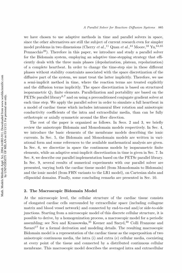
In this work, a parallel three-dimensional solver for numerical simulations in com-putational electrocardiology is introduced and studied. The solver is based on theanisotropic Bidomain cardiac model, consisting of a system of two degenerate parabolicreaction–diffusion equations describing the intra and extracellular potentials of themyocardial tissue. This model includes intramural fiber rotation and anisotropic con-ductivity coefficients that can be fully orthotropic or axially symmetric around thefiber direction. The solver also includes the simpler anisotropic Monodomain model,consisting of only one reaction–diffusion equation. These cardiac models are coupled witha membrane model for the ionic currents, consisting of a system of ordinary differentialequations that can vary from the simple FitzHugh–Nagumo (FHN) model to the morecomplex phase-I Luo–Rudy model (LR1). The solver employs structured isoparametricQ1 finite elements in space and a semi-implicit adaptive method in time. Parallelizationand portability are based on the PETSc parallel library. Large-scale computations withup to O(107) unknowns have been run on parallel computers, simulating excitation andrepolarization phenomena in three-dimensional domains.
Keywords: Reaction–diffusion equations; bidomain model; finite elements; parallel solver.
AMS Subject Classification: 65M60, 65M55
1. Introduction
The bioelectric activity of the heart is the subject of a vast interdisciplinary
literature in medicine, bioengineering, mathematical biology, physiology, chemistry
and physics; see the reference books by Zipes and Jalife,66 Panfilov and Holden,38
Keener and Sneyd30 and the references therein. Computational studies and nu-
merical simulations have played an important role in electrocardiology. Due to the
883
Mat
h. M
odel
s M
etho
ds A
ppl.
Sci.
2004
.14:
883-
911.
Dow
nloa
ded
from
ww
w.w
orld
scie
ntif
ic.c
omby
UN
IVE
RSI
TY
OF
MIL
AN
on
03/1
3/13
. For
per
sona
l use
onl
y.
May 31, 2004 15:27 WSPC/103-M3AS 00348
884 P. Colli Franzone & L. F. Pavarino
difficulty of direct measurements, many experimental studies have been coupled
with numerical investigations, even in medical and bioengineering works.
In particular attention has been paid to the computational study of re-entry
phenomena and their relationships with myocardial arrhythmias; see e.g. the special
issues1–3 and references therein.
The most complete model of cardiac electrical activity is the Bidomain model,
see e.g. Refs. 23 and 49. It consists of a system of two degenerate parabolic reaction–
diffusion equations describing the intra and extracellular potential in the cardiac
muscle, coupled with a system of ordinary differential equations describing the ionic
currents flowing through the cellular membrane. This model is computationally
expensive because of the involvement of different space and time scales. In fact,
meaningful portions of cardiac tissue have sizes of the order of centimeters, while
the steep potential gradient is localized in a thin layer about one millimeter thick,
requiring discretizations on the order of a tenth of millimeter. Moreover, a normal
heartbeat can last on the order of one second, while the time constants of the
rapid kinetics involved range from 0.1 to 500 milliseconds, requiring in some phases
time steps on the order of the hundredths of milliseconds (or less when currents or
shocks are applied). Therefore, in realistic three-dimensional models it is possible
to have discrete problems with more than O(107) unknowns at every time step and
simulations have to be run for many thousands of time steps.
A simplified cardiac tissue model is the anisotropic Monodomain system,
i.e. a parabolic reaction–diffusion equation describing the evolution of the trans-
membrane potential coupled with an ionic model. This model has been widely
used for three-dimensional simulations considering ionic models ranging from
simple FitzHugh–Nagumo (FHN) variants (Winfree,62,63 Rogers and McCulloch,47
Panfilov37) to the more complex phase-I Luo–Rudy (LR1) model,32 see e.g. Efimov
et al.,19 Rappel,46 Garfinkel et al.21
Previous Bidomain computations, mainly focusing on the excitation phase,
were performed on medium scale problems by Colli Franzone,12 Roth,48 Hooke
et al.,26 Henriquez et al.,23,24 Muzikant et al.34 These Bidomain studies of the
excitation phase, were able to reproduce the qualitative patterns and morpholo-
gies of the experimentally observed extracellular potential maps and electro-
grams (see e.g. Taccardi et al.,56 Colli Franzone et al.,14,15 Henriquez et al.,24
Muzikant et al.34).
A further reduction of the computational complexity of the simulation of
the excitation phase has been achieved by solving simplified kinematic models,
called eikonal equations, describing the motion of the excitation wave fronts, see
e.g. Colli Franzone et al.,12 Keener28 and Bellettini et al.8 On the other hand,
simplified approaches derived from reaction–diffusion models are not available at
present for the description of all the phases of an entire heartbeat.
Large-scale simulations of the whole heartbeat using Bidomain and Monodomain
models require adaptive and parallel tools in order to reduce their high computa-
tional cost. While both tools can in principle be applied to both space and time,
Mat
h. M
odel
s M
etho
ds A
ppl.
Sci.
2004
.14:
883-
911.
Dow
nloa
ded
from
ww
w.w
orld
scie
ntif
ic.c
omby
UN
IVE
RSI
TY
OF
MIL
AN
on
03/1
3/13
. For
per
sona
l use
onl
y.
May 31, 2004 15:27 WSPC/103-M3AS 00348
A Parallel Solver for Reaction–Diffusion Systems 885
we have chosen to use adaptive methods in time and parallel solvers in space,
since the other alternatives are still the subject of current research even for simpler
model problems in two dimensions (Cherry et al.,11 Quan et al.,44 Moore,33 Yu,64,65
Pennacchio39). Therefore in this paper, we introduce and study a parallel solver
for the Bidomain system, employing an adaptive time-stepping strategy that effi-
ciently deals with the three main phases (depolarization, plateau, repolarization)
of a complete heartbeat. In order to change the time-step size in these different
phases without stability constraints associated with the space discretization of the
diffusive part of the system, we must treat the latter implicitly. Therefore, we use
a semi-implicit method in time, where the reaction terms are treated explicitly
and the diffusion terms implicitly. The space discretization is based on structured
isoparametric Q1 finite elements. Parallelization and portability are based on the
PETSc parallel library6,7 and on using a preconditioned conjugate gradient solver at
each time step. We apply the parallel solver in order to simulate a full heartbeat in
a model of cardiac tissue which includes intramural fiber rotation and anisotropic
conductivity coefficients of the intra and extracellular media, than can be fully
orthotropic or axially symmetric around the fiber direction.
The rest of the paper is organized as follows. In Secs. 2 and 3, we briefly
review the anisotropic Bidomain and Monodomain models respectively. In Sec. 4,
we introduce the basic elements of the membrane models describing the ionic
currents. In Sec. 5, the Bidomain and Monodomain models are written in vari-
ational form and some references to the available mathematical analysis are given.
In Sec. 6, we discretize in space the continuous models by isoparametric finite
elements, while an adaptive semi-implicit discretization in time is given in Sec. 7. In
Sec. 8, we describe our parallel implementation based on the PETSc parallel library.
In Sec. 9, several results of numerical experiments with our parallel solver are
presented, varying both the cardiac tissue model (from Monodomain to Bidomain)
and the ionic model (from FHN variants to the LR1 model), on Cartesian slabs and
ellipsoidal domains. Finally, some concluding remarks are presented in Sec. 10.
2. The Macroscopic Bidomain Model
At the microscopic level, the cellular structure of the cardiac tissue consists
of elongated cardiac cells surrounded by extracellular space (including collagene
matrix and blood vessel network) and connected by end-to-end and/or side-to-side
junctions. Starting from a microscopic model of this discrete cellular structure, it is
possible to derive, by a homogenization process, a macroscopic model for a periodic
assembling; see Neu and Krassowska,35 Keener and Sneyd,30 Colli Franzone and
Savare17 for a formal derivation and modeling details. The resulting macroscopic
Bidomain model is a representation of the cardiac tissue as the superposition of two
anisotropic continuous media, the intra (i) and extra (e) cellular media, coexisting
at every point of the tissue and connected by a distributed continuous cellular
membrane. This macroscopic model describes the averaged intra and extracellular
Mat
h. M
odel
s M
etho
ds A
ppl.
Sci.
2004
.14:
883-
911.
Dow
nloa
ded
from
ww
w.w
orld
scie
ntif
ic.c
omby
UN
IVE
RSI
TY
OF
MIL
AN
on
03/1
3/13
. For
per
sona
l use
onl
y.

May 31, 2004 15:27 WSPC/103-M3AS 00348
886 P. Colli Franzone & L. F. Pavarino
A
B
C
D
E
Fig. 1. Fiber direction on epicardium (A), a mid-wall layer (B), endocardium (C), a meridiansection (D) and a transverse section (E).
electric potentials and currents by a reaction–diffusion system of degenerate
parabolic type.
Let Ω ⊂ R3 be the bounded physical region occupied by the cardiac tissue.
In the macroscopic Bidomain representation of the cardiac tissue, the anisotropic
structure of the two averaged continuous media, the intra and the extracellular
medium, are characterized by the conductivity tensors Di and De. The anisotropic
conductivity is related to the arrangement of the cardiac fibers, whose direction
rotates counterclockwise from the epicardium (outer heart surface) to the endo-
cardium (inner surface); see Fig. 1. We refer to Streeter54 and Peskin41 for an experi-
mental and mathematical study of this fiber structure. Recently Le Grice et al.31
have shown that the ventricular myocardium may be conceived as a set of muscle
sheets running radially from epicardium to endocardium. In this laminar organi-
zation, it is possible to identify three distinct principal axes at any point x. Let
al(x), at(x), an(x) be a triplet of orthonormal vectors related to the structure of the
myocardium at a point x, with al parallel to the local fiber direction and an normal
to the muscle sheet. This triplet may depend on the position x in the myocardium.
Let σi,el , σi,e
t , σi,en be the conductivity coefficients measured along the corresponding
directions. In general, these coefficients may depend on x, but in the following we
assume that they are constant, i.e. homogeneous anisotropy. Then the conductivity
tensors Di and De, generally dependent on the position x, are given by:
Di,e(x) = σi,el al(x)aT
l (x) + σi,et at(x)aT
t (x) + σi,en an(x)aT
n (x) . (2.1)
If σi,en = σi,e
t , we recover the axially isotropic case
Di,e(x) = σi,et I + (σi,e
l − σi,et )al(x)aT
l (x) .
The biolelectric activity of cardiac cells is due to the flow Iion (per unit area of the
membrane surface) of various ionic currents (the most important being sodium,
Mat
h. M
odel
s M
etho
ds A
ppl.
Sci.
2004
.14:
883-
911.
Dow
nloa
ded
from
ww
w.w
orld
scie
ntif
ic.c
omby
UN
IVE
RSI
TY
OF
MIL
AN
on
03/1
3/13
. For
per
sona
l use
onl
y.

May 31, 2004 15:27 WSPC/103-M3AS 00348
A Parallel Solver for Reaction–Diffusion Systems 887
potassium and calcium) through the cellular membrane. Since the membrane
behaves as a capacitor, the total membrane current per unit volume is given by
Im = χ
(
Cm
∂v
∂t+ Iion
)
,
where v = ui − ue is the transmembrane potential, the coefficient χ is the ratio of
membrane area per tissue volume, Cm is the surface capacitance of the membrane,
and Iion(v, w) is the ionic current described later and depending on the membrane
model employed.
Imposing the conservation of currents, i.e. the interchange between the two
media must balance the membrane current flow per unit volume, we have divJi =
−divJe = Im, where Ji,e = −Di,e∇ui,e are the intra and extracellular current
densities. Therefore, in the Bidomain model, the intra and extracellular potentials
ui, ue are modeled by the following reaction–diffusion system of PDEs, coupled
with a system of ODEs for M gating variables and ion concentrations modeling
the ionic currents, described later. Given an applied current per unit volume I i,eapp :
Ω × (0, T ) −→ R, initial conditions v0 : Ω −→ R, w0 : Ω −→ RM , find the intra
and extracellular potentials ui, ue : Ω × (0, T ) −→ R, the transmembrane potential
v = ui − ue and the gating and concentration variables w : Ω× (0, T ) −→ RM such
that
χCm
∂v
∂t− div(Di∇ui) + χIion(v, w) = I i
app in Ω × (0, T )
−χCm
∂v
∂t− div(De∇ue) − χIion(v, w) = −Ie
app in Ω × (0, T )
∂w
∂t−R(v, w) = 0 , v(x, t) = ui(x, t) − ue(x, t) in Ω × (0, T ) .
(2.2)
In the following, we assume that the cardiac tissue is insulated, therefore homoge-
neous Neumann boundary conditions are assigned on ∂Ω × (0, T )
nTDi∇ui = 0 , nTDe∇ue = 0 .
Initial conditions (degenerate for ui and ue) are assigned in Ω for t = 0
v(x, 0) = ui(x, 0) − ue(x, 0) = v0(x) , w(x, 0) = w0(x) . (2.3)
Adding the two equations of the system, we have −divDi∇ui −divDe∇ue = I iapp −
Ieapp. Integrating on Ω and applying the divergence theorem, from the Neumann
boundary conditions, we then have the following compatibility condition for the
system (2.2) to be solvable:∫
Ω
I iappdx =
∫
Ω
Ieappdx . (2.4)
We recall that electric potentials in bounded domains are defined up to an ad-
ditive constant; in our case ui and ue are determined up to the same additive
time-dependent constant, while v is uniquely determined. This common constant is
Mat
h. M
odel
s M
etho
ds A
ppl.
Sci.
2004
.14:
883-
911.
Dow
nloa
ded
from
ww
w.w
orld
scie
ntif
ic.c
omby
UN
IVE
RSI
TY
OF
MIL
AN
on
03/1
3/13
. For
per
sona
l use
onl
y.

May 31, 2004 15:27 WSPC/103-M3AS 00348
888 P. Colli Franzone & L. F. Pavarino
related to the choice of a reference potential. The usual choice consists of selecting
this constant so that ue has zero average on Ω, i.e.∫
Ω
uedx = 0 . (2.5)
3. The Simplified Monodomain Model
Assuming equal anisotropy ratio of the two media, i.e. Di = λDe with λ constant,
and setting D = λDi
1+λand Iapp =
λIiapp
1+λ+
Ieapp
1+λ, then the Bidomain system reduces
to the anisotropic Monodomain model consisting in a parabolic reaction–diffusion
equation for the transmembrane potential v only
χCm
∂v
∂t− div(D(x)∇v) + χIion(v, w) = Iapp , in Ω × (0, T )
∂w
∂t−R(v, w) = 0 in Ω × (0, T ) ,
(3.1)
with Neumann boundary conditions for v and initial conditions for v and w. The
conductivity tensor in the axial symmetric case is given by
D(x) = σl al(x)aTl (x)+σt at(x)aT
t (x)+σn an(x)aTn (x) with σl,t,n =
λ
1 + λσi
l,t,n .
This model has been vastly used in computational electrocardiology because it
requires substantially less computational and memory resources than the Bidomain
model. Nevertheless, it is not an adequate cardiac model since it is unable to repro-
duce some patterns and morphology of the experimentally observed extracellular
potential maps and electrograms; see Colli Franzone et al.,14 Henriquez et al.,24
Muzikant et al.34 Therefore, unequal anisotropy ratio of the intra and extracellular
media cannot be neglected.
4. Membrane Models and Ionic Currents
The first membrane model for ionic currents was given in the celebrated work
on nerve action potential by Hodgkin and Huxley,25 work that earned them the
Nobel prize in Medicine in 1963. Models of Hodgkin–Huxley type have been later
developed for the cardiac action potential. In these models, the ionic current through
channels of the membrane, due to the transmembrane potential v and M gating
and ionic concentration variables w := (w1, . . . , wM ), is given by
Iion(v, w) =
N∑
k=1
Gk(v)
M∏
j=1
wpjk
j (v − vk(w)) ,
where Gk(v) is the membrane conductance, vk is the reversal potential for the kth
current and pjkare integers. The dynamics of the gating and concentration variables
is described by the system of ODE’s
∂w
∂t= R(v, w) , w(x, 0) = w0(x) .
Mat
h. M
odel
s M
etho
ds A
ppl.
Sci.
2004
.14:
883-
911.
Dow
nloa
ded
from
ww
w.w
orld
scie
ntif
ic.c
omby
UN
IVE
RSI
TY
OF
MIL
AN
on
03/1
3/13
. For
per
sona
l use
onl
y.
May 31, 2004 15:27 WSPC/103-M3AS 00348
A Parallel Solver for Reaction–Diffusion Systems 889
0 100 200 300 400
0
25
50
75
100
MSEC.
mV
(a)
0 100 200 300 400
−80
−40
0
MSEC
mV
(b)
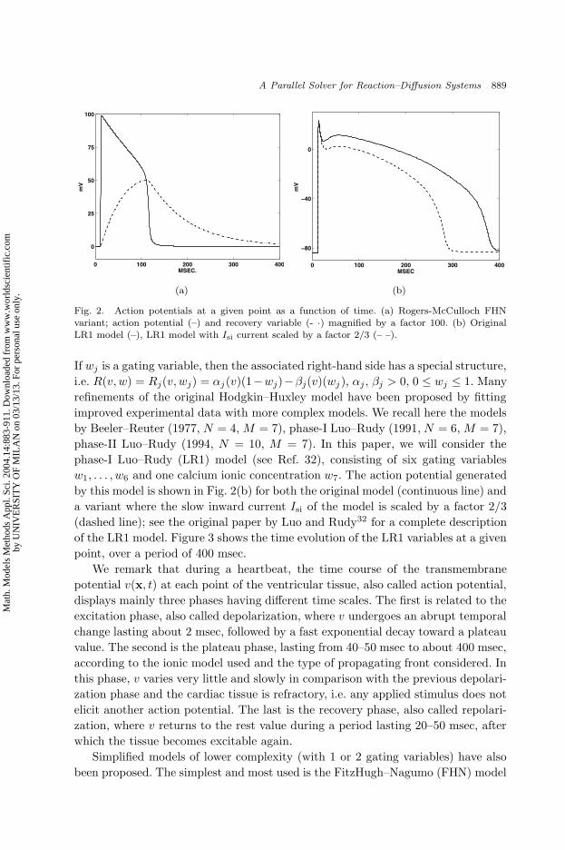
Fig. 2. Action potentials at a given point as a function of time. (a) Rogers-McCulloch FHNvariant; action potential (–) and recovery variable (- ·) magnified by a factor 100. (b) OriginalLR1 model (–), LR1 model with Isi current scaled by a factor 2/3 (– –).
If wj is a gating variable, then the associated right-hand side has a special structure,
i.e. R(v, w) = Rj(v, wj) = αj(v)(1−wj)−βj(v)(wj ), αj , βj > 0, 0 ≤ wj ≤ 1. Many
refinements of the original Hodgkin–Huxley model have been proposed by fitting
improved experimental data with more complex models. We recall here the models
by Beeler–Reuter (1977, N = 4, M = 7), phase-I Luo–Rudy (1991, N = 6, M = 7),
phase-II Luo–Rudy (1994, N = 10, M = 7). In this paper, we will consider the
phase-I Luo–Rudy (LR1) model (see Ref. 32), consisting of six gating variables
w1, . . . , w6 and one calcium ionic concentration w7. The action potential generated
by this model is shown in Fig. 2(b) for both the original model (continuous line) and
a variant where the slow inward current Isi of the model is scaled by a factor 2/3
(dashed line); see the original paper by Luo and Rudy32 for a complete description
of the LR1 model. Figure 3 shows the time evolution of the LR1 variables at a given
point, over a period of 400 msec.
We remark that during a heartbeat, the time course of the transmembrane
potential v(x, t) at each point of the ventricular tissue, also called action potential,
displays mainly three phases having different time scales. The first is related to the
excitation phase, also called depolarization, where v undergoes an abrupt temporal
change lasting about 2 msec, followed by a fast exponential decay toward a plateau
value. The second is the plateau phase, lasting from 40–50 msec to about 400 msec,
according to the ionic model used and the type of propagating front considered. In
this phase, v varies very little and slowly in comparison with the previous depolari-
zation phase and the cardiac tissue is refractory, i.e. any applied stimulus does not
elicit another action potential. The last is the recovery phase, also called repolari-
zation, where v returns to the rest value during a period lasting 20–50 msec, after
which the tissue becomes excitable again.
Simplified models of lower complexity (with 1 or 2 gating variables) have also
been proposed. The simplest and most used is the FitzHugh–Nagumo (FHN) model
Mat
h. M
odel
s M
etho
ds A
ppl.
Sci.
2004
.14:
883-
911.
Dow
nloa
ded
from
ww
w.w
orld
scie
ntif
ic.c
omby
UN
IVE
RSI
TY
OF
MIL
AN
on
03/1
3/13
. For
per
sona
l use
onl
y.

May 31, 2004 15:27 WSPC/103-M3AS 00348
890 P. Colli Franzone & L. F. Pavarino
0 100 200 300 400−100
−50
0
v
0 100 200 300 400−0.5
0
0.5
1
1.5
m g
ate
(w
1)
0 100 200 300 400−0.5
0
0.5
1
1.5
h g
ate
(w
2)
0 100 200 300 400−0.5
0
0.5
1
1.5
j gate
(w
3)
0 100 200 300 400−0.5
0
0.5
1
1.5
d g
ate
(w
4)
0 100 200 300 400−0.5
0
0.5
1
1.5
f gate
(w
5)
0 100 200 300 400−0.1
0
0.1
0.2
MSEC
X g
ate
(w
6)
0 100 200 300 4000
2
4
x 10−3
MSEC
Ca
i gate
(w
7)
Fig. 3. LR1 membrane model: action potential v, gating variables w1, . . . , w6, calcium concen-tration w7 at a given point as a function of time.
(N = 1, M = 1). Assuming that at rest the potential v is zero, in this model the
ionic current is described using only one recovery variable w
Iion(v, w) = g(v) + βw ,
where β > 0, g is a cubic-like function and w satisfies
R(v, w) = ηv − γw ,
with η, γ > 0. The FHN gating model yields only a coarse approximation of a typical
cardiac action potential, particularly in the plateau and repolarization phases. A
better approximation is given by the following variant by Rogers and McCulloch47
Iion(v, w) = Gv
(
1 −v
vth
)(
1 −v
vp
)
+ η1vw ,
∂w
∂t= η2
(
v
vp− η3w
)
,
where G, η1, η2, η3 are positive real coefficients, vth is a threshold potential and vpthe peak potential. We will consider this variant as our simplest gating model. The
action potential generated with this model is plotted in Fig. 2(a) (continuous line),
together with the recovery variable w magnified by a factor 100 (dash-dotted line).
A more recent simplified ionic model with three currents and two gating variables
was extensively investigated by Fenton and Karma.20
Mat
h. M
odel
s M
etho
ds A
ppl.
Sci.
2004
.14:
883-
911.
Dow
nloa
ded
from
ww
w.w
orld
scie
ntif
ic.c
omby
UN
IVE
RSI
TY
OF
MIL
AN
on
03/1
3/13
. For
per
sona
l use
onl
y.
May 31, 2004 15:27 WSPC/103-M3AS 00348
A Parallel Solver for Reaction–Diffusion Systems 891
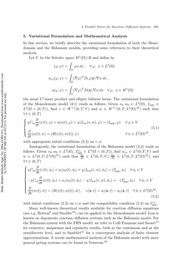
5. Variational Formulation and Mathematical Analysis
In this section, we briefly describe the variational formulation of both the Mono-
domain and the Bidomain models, providing some references to their theoretical
analysis.
Let V be the Sobolev space H1(Ω)/R and define by
(ϕ, ψ) =
∫
Ω
ϕψ dx , ∀ϕ, ψ ∈ L2(Ω)
ai,e(ϕ, ψ) =
∫
Ω
(∇ϕ)TDi,e(x)∇ψ dx ,
a(ϕ, ψ) =
∫
Ω
(∇ϕ)TD(x)∇ψ dx ∀ϕ, ψ ∈ H1(Ω)
the usual L2-inner product and elliptic bilinear forms. The variational formulation
of the Monodomain model (3.1) reads as follows. Given v0, w0 ∈ L2(Ω), Iapp ∈
L2(Ω × (0, T )), find v ∈ W 1,1(0, T ;V ) and w ∈ W 1,1(0, T ;L2(Ω)M ) such that
∀ t ∈ (0, T )
χCm
∂
∂t(v(t), ϕ) + a(v(t), ϕ) + χ(Iion(v, w), ϕ) = (Iapp, ϕ) ∀ϕ ∈ V
∂
∂t(w(t), ψ) = (R(v(t), w(t)), ψ) ∀ψ ∈ L2(Ω)M ,
(5.1)
with appropriate initial conditions (2.3) on v, w.
Analogously, the variational formulation of the Bidomain model (2.2) reads as
follows. Given v0, w0 ∈ L2(Ω), I i,eapp ∈ L2(Ω × (0, T )), find ui,e ∈ L2(0, T ;V ) and
w ∈ L2(0, T ;L2(Ω)M ) such that ∂v∂t
∈ L2(0, T ;V ), ∂w∂t
∈ L2(0, T ;L2(Ω)M ), and
∀ t ∈ (0, T )
χCm
∂
∂t(v(t), ui) + ai(ui(t), ui) + χ(Iion(v, w), ui) = (I i
app, ui) ∀ ui ∈ V
−χCm
∂
∂t(v(t), ue) + ae(ue(t), ue) − χ(Iion(v, w), ue) = −(Ie
app, ue) ∀ ue ∈ V
∂
∂t(w(t), w) = (R(v(t), w(t)), w) , v(x, t) = ui(x, t) − ue(x, t) ∀ w ∈ L2(Ω)M ,
(5.2)
with initial conditions (2.3) on v, w and the compatibility condition (2.4) on I i,eapp.
Many well-known theoretical results available for reaction–diffusion equations
(see e.g. Britton9 and Smoller53) can be applied to the Monodomain model. Less is
known on degenerate reaction–diffusion systems such as the Bidomain model. For
the Bidomain system with the FHN model, we refer to Colli Franzone and Savare17
for existence, uniqueness and regularity results, both at the continuous and at the
semidiscrete level, and to Sanfelici51 for a convergence analysis of finite element
approximations. A recent mathematical analysis of the Bidomain model with more
general gating systems can be found in Veneroni.59
Mat
h. M
odel
s M
etho
ds A
ppl.
Sci.
2004
.14:
883-
911.
Dow
nloa
ded
from
ww
w.w
orld
scie
ntif
ic.c
omby
UN
IVE
RSI
TY
OF
MIL
AN
on
03/1
3/13
. For
per
sona
l use
onl
y.

May 31, 2004 15:27 WSPC/103-M3AS 00348
892 P. Colli Franzone & L. F. Pavarino
More results are known on the related eikonal approximation describing the
propagation of the excitation front; we refer to Colli Franzone et al.,12,13 Keener28
and Bellettini et al.8 A mathematical analysis of the Bidomain model using Γ-
convergence theory can be found in Ambrosio et al.4
6. Finite Element Discretization in Space
We will use hexahedral isoparametricQ1 finite elements in space; see e.g. Quarteroni
and Valli45 for a general introduction to the finite element method. Our domain
Ω representing the left ventricle is modeled by a family of truncated ellipsoids
described by the parametric equations
x = a(r) cos θ cosφ φmin ≤ φ ≤ φmax ,
y = b(r) cos θ sinφ θmin ≤ θ ≤ θmax ,
z = c(r) sin θ 0 ≤ r ≤ 1 ,
(6.1)
where a(r) = a1 + r(a2 − a1), b(r) = b1 + r(b2 − b1), c(r) = c1 + r(c2 − c1), and
ai, bi, ci, i = 1, 2 are given coefficients determining the main axes of the ellipsoid. As
in Ref. 13, the fibers rotate intramurally linearly with the depth for a total amount
of 120 proceeding counterclockwise from epicardium to endocardium; see Fig. 1.
More precisely, in a local ellipsoidal reference system (eφ, eθ, er), the fiber direction
al(x) at a point x is given by
al(x) = eφ cosα(r) + eθ sinα(r) , with α(r) =2
3π(1 − r) −
π
4, 0 ≤ r ≤ 1 .
To take into account the obliqueness of al with respect to the ellipsoidal surfaces, we
introduce, besides α(r), the “oblique” angle β (known as imbrication angle) which
describes the deviation of al from the tangent position. For more details about
the imbrication angle and the fiber pathways, see Ref. 13. We also consider three-
dimensional slabs of cardiac tissue, described in the usual Cartesian coordinate
system by
x = a(r)
y = b(r)
z = c(r)
with
al(x) = ex cosα(r) + ey sinα(r) ,
α(r) = α0π(1 − r) −π
4, 0 ≤ r ≤ 1 .
(6.2)
The domain Ω is discretized by introducing a structured quasi-uniform grid of
hexahedral isoparametric Q1 elements obtained by a uniform subdivision of the in-
tervals [φmin, φmax], [θmin, θmax], [0, 1] into (nφ, nθ, nr) subintervals. Using the same
symbol Ω for the domain and its FEM approximation, we have Ω =⋃
E∈ThE,
where E = TE(E), with E = [−1, 1]3 and TE a trilinear map. The associated finite
element space is given by
Vh = ϕh ∈ V : ϕh is continuous in Ω : ϕh|E TE ∈ Q1(E) , ∀E ∈ Th ,
Mat
h. M
odel
s M
etho
ds A
ppl.
Sci.
2004
.14:
883-
911.
Dow
nloa
ded
from
ww
w.w
orld
scie
ntif
ic.c
omby
UN
IVE
RSI
TY
OF
MIL
AN
on
03/1
3/13
. For
per
sona
l use
onl
y.

May 31, 2004 15:27 WSPC/103-M3AS 00348
A Parallel Solver for Reaction–Diffusion Systems 893
where Q1(E) is the space of the trilinear functions on E. A semidiscrete problem is
obtained by applying a standard Galerkin procedure and choosing a finite element
basis φi for Vh. Let M = (mrs), A = (ars) and Ai,e = (ai,ers) be the symmetric
mass and stiffness matrices defined by
mrs =∑
E
∫
E
ϕr ϕsdx ,
ars =∑
E
∫
E
(∇ϕr)TD(x)∇ϕsdx , ai,e
rs =∑
E
∫
E
(∇ϕr)TDi,e(x)∇ϕsdx .
Numerical quadrature with a simple trapezoidal rule in three dimensions is used
in order to compute these integrals. Let Ihion, I
happ, I
i,happ, I
e,happ be the finite element
interpolants of Iion, Iapp, Iiapp, I
eapp, respectively. In the following, we will denote by
the same letters finite element functions and the vectors of their nodal values. In
the Monodomain model, the finite element approximation vh of the transmembrane
potential is the solution of
χCmM∂vh
∂t+ Avh + χM Ihion(vh,wh) = M Ihapp , (6.3)
while in the Bidomain model, the finite element approximations ui,h,ue,h of the
intra and extracellular potentials are the solutions of the system
χCmM∂vh
∂t+ Aiui,h + χM Ihion(vh,wh) = M Ii,happ ,
−χCmM∂vh
∂t+ Aeue,h − χM Ihion(vh,wh) = −M Ie,h
app ,
(6.4)
where vh = ui,h−ue,h. In both cases, these equations are coupled with the semidis-
crete approximations of the gating and concentration system
∂wh
∂t= R(vh,wh) .
The Bidomain system can be written in compact form as
χCmM∂
∂t
(
ui,h
ue,h
)
+ A
(
ui,h
ue,h
)
+ χ
(
M Ihion(vh,wh)
−M Ihion(vh,wh)
)
=
(
M Ii,happ
−M Ie,happ
)
,
(6.5)
where
M =
[
M −M
−M M
]
, A =
[
Ai 0
0 Ae
]
.
The Bidomain system (6.4) can alternatively be written in terms of vh,ue,h by
adding the two equations and substituting ui,h = vh + ue,h into the first equation,
Mat
h. M
odel
s M
etho
ds A
ppl.
Sci.
2004
.14:
883-
911.
Dow
nloa
ded
from
ww
w.w
orld
scie
ntif
ic.c
omby
UN
IVE
RSI
TY
OF
MIL
AN
on
03/1
3/13
. For
per
sona
l use
onl
y.
May 31, 2004 15:27 WSPC/103-M3AS 00348
894 P. Colli Franzone & L. F. Pavarino
obtaining
χCmM∂vh
∂t+ Aivh + Aiue,h + χM Ihion(vh,wh) = M Ii,happ ,
Aivh + (Ae + Ai)ue,h = M(Ii,happ − Ie,happ) .
(6.6)
In the language of Differential-Algebraic equations (DAE), this formulation sepa-
rates the differential variable (vh) from the algebraic variable (ue,h); it was first
used in Refs. 12 and 48 and subsequently by many others, e.g. Refs. 10, 24, 26,
27, 29, 34, 55 and 58. Finally, another numerical approach21,43 has been recently
applied to the Monodomain model using a splitting of the diffusion and reaction
operators.
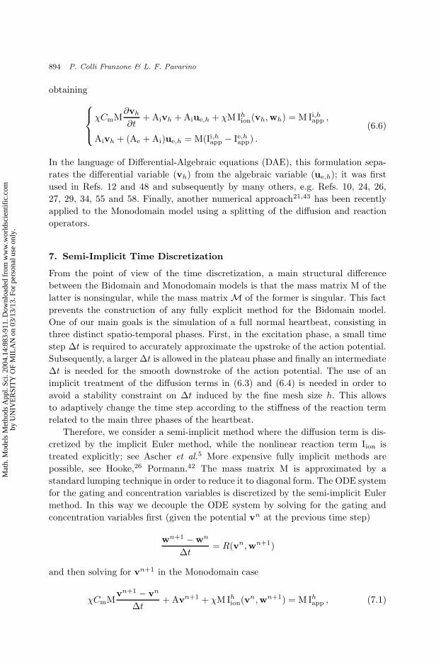
7. Semi-Implicit Time Discretization
From the point of view of the time discretization, a main structural difference
between the Bidomain and Monodomain models is that the mass matrix M of the
latter is nonsingular, while the mass matrix M of the former is singular. This fact
prevents the construction of any fully explicit method for the Bidomain model.
One of our main goals is the simulation of a full normal heartbeat, consisting in
three distinct spatio-temporal phases. First, in the excitation phase, a small time
step ∆t is required to accurately approximate the upstroke of the action potential.
Subsequently, a larger ∆t is allowed in the plateau phase and finally an intermediate
∆t is needed for the smooth downstroke of the action potential. The use of an
implicit treatment of the diffusion terms in (6.3) and (6.4) is needed in order to
avoid a stability constraint on ∆t induced by the fine mesh size h. This allows
to adaptively change the time step according to the stiffness of the reaction term
related to the main three phases of the heartbeat.
Therefore, we consider a semi-implicit method where the diffusion term is dis-
cretized by the implicit Euler method, while the nonlinear reaction term Iion is
treated explicitly; see Ascher et al.5 More expensive fully implicit methods are
possible, see Hooke,26 Pormann.42 The mass matrix M is approximated by a
standard lumping technique in order to reduce it to diagonal form. The ODE system
for the gating and concentration variables is discretized by the semi-implicit Euler
method. In this way we decouple the ODE system by solving for the gating and
concentration variables first (given the potential vn at the previous time step)
wn+1 −wn
∆t= R(vn,wn+1)
and then solving for vn+1 in the Monodomain case
χCmMvn+1 − vn
∆t+ Avn+1 + χM Ihion(v
n,wn+1) = M Ihapp , (7.1)
Mat
h. M
odel
s M
etho
ds A
ppl.
Sci.
2004
.14:
883-
911.
Dow
nloa
ded
from
ww
w.w
orld
scie
ntif
ic.c
omby
UN
IVE
RSI
TY
OF
MIL
AN
on
03/1
3/13
. For
per
sona
l use
onl
y.

May 31, 2004 15:27 WSPC/103-M3AS 00348
A Parallel Solver for Reaction–Diffusion Systems 895
or for un+1i ,un+1
e in the Bidomain case
χCmMvn+1 − vn
∆t+ Aiu
n+1i + χM Ihion(v
n,wn+1) = M Ii,happ ,
−χCmMvn+1 − vn
∆t+ Aeu
n+1e − χM Ihion(vn,wn+1) = −M Ie,h
app ,
(7.2)
where vn = uni − un
e . Alternatively, one could solve for the potentials first (given
the gating and concentration variables at the previous time step) and then solve for
the new gating and concentration variables. The resulting semi-implicit iterative
method in the Monodomain case (7.1) is(
χCm
∆tM + A
)
vn+1 =χCm
∆tMvn − χM Ihion(vn,wn+1) + M Ihapp , (7.3)
while the Bidomain case (7.2) can be written, in terms of the iteration matrix,
i.e. the weighted sum of mass and stiffness matrices, as(
χCm
∆t
[
M −M
−M M
]
+
[
Ai 0
0 Ae
])(
un+1i
un+1e
)
=χCm
∆t
[
M −M
−M M
](
uni
une
)
−χ
(
M Ihion(vn,wn+1)
−M Ihion(vn,wn+1)
)
+
(
M Ii,happ
−M Ie,happ
)
. (7.4)
We assign the initial conditions u0i = −84 mV and u0
e = 0 mV, so that v0 =
−84 mV. As in the continuous model, vn is uniquely determined by the given initial
and boundary conditions, while uni and un
e are determined only up to the same
additive time-dependent constant related to a reference potential. Since we con-
sider bounded domains, we can determine this constant by imposing the condition
1TMune = 0.
We remark that this semi-implicit treatment leads to a linear system at each time
step in (7.3) with a symmetric positive definite iteration matrix, while the linear
system in (7.4) involves a symmetric positive semidefinite iteration matrix, with
a one-dimensional kernel spanned by (1,1)T. These systems are solved iteratively
by the preconditioned conjugate gradient (PCG) method, using as initial guess
the solution at the previous time step. More details on the parallel linear solver
are given in the next section. The extension of the recent Monodomain operator
splitting techniques21,43 to the Bidomain model would lead to a linear parabolic
system χCmM∂u
∂t+ Au = 0, with u = (ui,h,ue,h)T. The iteration matrix arising
from the implicit discretization of this system coincides with the iteration matrix
in (7.4) and therefore we would have the same computational complexity at each
time step.
Mat
h. M
odel
s M
etho
ds A
ppl.
Sci.
2004
.14:
883-
911.
Dow
nloa
ded
from
ww
w.w
orld
scie
ntif
ic.c
omby
UN
IVE
RSI
TY
OF
MIL
AN
on
03/1
3/13
. For
per
sona
l use
onl
y.

May 31, 2004 15:27 WSPC/103-M3AS 00348
896 P. Colli Franzone & L. F. Pavarino
The adaptive time-stepping strategy employed is based on controlling the trans-
membrane potential variation ∆v = max(vn+1−vn) at each time step; see Refs. 26,
32, 36 and 60. In short, the adaptive strategy is the following:
if ∆v < ∆vmin = 0.05, then ∆tnew = ∆vmax
∆v∆told (if ∆tnew < ∆tmax = 6 msec);
if ∆v > ∆vmax = 0.5, then ∆tnew = ∆vmin
∆v∆told (if ∆tnew > ∆tmin = 0.005 msec).
Due to the linearity of the gating equation for wj , in the Hodgkin–Huxley
formalism the equations can be written as
∂wj
∂t=
wj∞ −wj
τwj
, on (0,∆t) , with wj(x, 0) = wnj (x)
wj∞(vn) = αj(vn)τwj
(vn) , τwj(vn) =
1
αj(vn) + βj(vn).
In order to also guarantee a control on the variation of the gating variables wj ,
they are integrated exactly given v (see Victorri et al.,60) i.e.
wn+1j = wj∞(vn) + (wn
j −wj∞(vn)) exp(−∆t/τwj(vn)) .
In particular, in the LR1 ionic model, the update of the gating variables w1, . . . , w6
are based on the previous explicit formula; using these values the calcium concen-
tration w7 is then updated applying the implicit Euler method.
8. Parallel Implementation and Computational Costs
In order to reduce the high computational cost of large-scale simulations of the
whole heartbeat solving (7.3) and (7.4) at each time step, we have chosen to use
adaptive methods in time, described before, and parallel solvers in space. Among
other works using parallel tools in cardiac simulations, see Refs. 21, 42, 44, 50
and 61. Our strategy for building an efficient parallel solver is based on using the
parallel library PETSc from Argonne National Laboratory; see Refs. 6 and 7. This
library, built on the MPI standard, offers advanced data structures and routines
for the parallel solution of partial differential equations, from basic vector and
matrix operations to more complex linear and nonlinear equation solvers. In our
FORTRAN code, the necessary vectors and matrices are built and subassembled
in parallel on each processor and then the solution is advanced in time on each
processor in a synchronous manner. In order to minimize the bandwidth of the
stiffness matrix (as in Refs. 26 and 40) and to improve data locality in PETSc,
we have reordered the unknowns writing for every node the ui and ue components
consecutively. This allows us to take full advantage of the parallel objects in the
PETSc library, such as the Distributed Arrays (DA) objects, where the couple ui,
ue is associated with each node of the structured mesh. At each time step, the main
computational costs are associated with
Mat
h. M
odel
s M
etho
ds A
ppl.
Sci.
2004
.14:
883-
911.
Dow
nloa
ded
from
ww
w.w
orld
scie
ntif
ic.c
omby
UN
IVE
RSI
TY
OF
MIL
AN
on
03/1
3/13
. For
per
sona
l use
onl
y.

May 31, 2004 15:27 WSPC/103-M3AS 00348
A Parallel Solver for Reaction–Diffusion Systems 897
0 300 600 900 1200 1500 180010
−7
10−6
10−5
10−4
10−3
10−2
10−1
100
MONODOMAIN
BIDOMAIN
EIG
EN
VA
LU
ES
(a)
0 300 600 900 1200 1500 180010
−6
10−5
10−4
10−3
10−2
10−1
100
BIDOMAIN
MONODOMAIN
EIG
EN
VA
LU
ES
(b)
Fig. 4. Nonzero eigenvalues of the stiffness matrices A and A related to elliptic operators with(a) homogeneous Neumann boundary conditions and (b) of the iteration matrices in (7.3) and(7.4). Monodomain eigenvalues, denoted by dots (·), are related to 15×15×8 = 1800 meshpoints.Bidomain eigenvalues, denoted by circles (o), are related to 15 × 15 × 4 meshpoints.
Mat
h. M
odel
s M
etho
ds A
ppl.
Sci.
2004
.14:
883-
911.
Dow
nloa
ded
from
ww
w.w
orld
scie
ntif
ic.c
omby
UN
IVE
RSI
TY
OF
MIL
AN
on
03/1
3/13
. For
per
sona
l use
onl
y.
May 31, 2004 15:27 WSPC/103-M3AS 00348
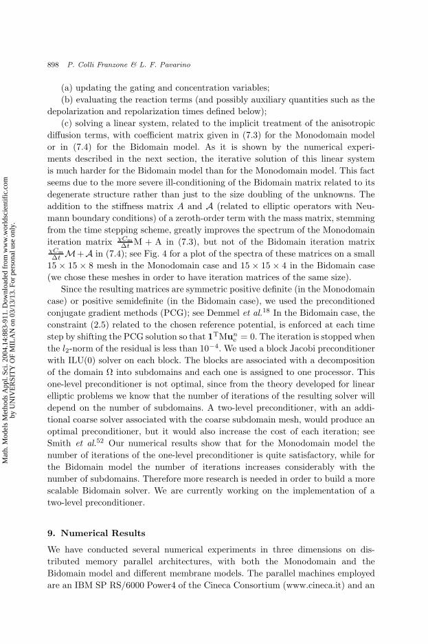
898 P. Colli Franzone & L. F. Pavarino
(a) updating the gating and concentration variables;
(b) evaluating the reaction terms (and possibly auxiliary quantities such as the
depolarization and repolarization times defined below);
(c) solving a linear system, related to the implicit treatment of the anisotropic
diffusion terms, with coefficient matrix given in (7.3) for the Monodomain model
or in (7.4) for the Bidomain model. As it is shown by the numerical experi-
ments described in the next section, the iterative solution of this linear system
is much harder for the Bidomain model than for the Monodomain model. This fact
seems due to the more severe ill-conditioning of the Bidomain matrix related to its
degenerate structure rather than just to the size doubling of the unknowns. The
addition to the stiffness matrix A and A (related to elliptic operators with Neu-
mann boundary conditions) of a zeroth-order term with the mass matrix, stemming
from the time stepping scheme, greatly improves the spectrum of the Monodomain
iteration matrix χCm
∆tM + A in (7.3), but not of the Bidomain iteration matrix
χCm
∆tM+A in (7.4); see Fig. 4 for a plot of the spectra of these matrices on a small
15 × 15 × 8 mesh in the Monodomain case and 15 × 15 × 4 in the Bidomain case
(we chose these meshes in order to have iteration matrices of the same size).
Since the resulting matrices are symmetric positive definite (in the Monodomain
case) or positive semidefinite (in the Bidomain case), we used the preconditioned
conjugate gradient methods (PCG); see Demmel et al.18 In the Bidomain case, the
constraint (2.5) related to the chosen reference potential, is enforced at each time
step by shifting the PCG solution so that 1TMune = 0. The iteration is stopped when
the l2-norm of the residual is less than 10−4. We used a block Jacobi preconditioner
with ILU(0) solver on each block. The blocks are associated with a decomposition
of the domain Ω into subdomains and each one is assigned to one processor. This
one-level preconditioner is not optimal, since from the theory developed for linear
elliptic problems we know that the number of iterations of the resulting solver will
depend on the number of subdomains. A two-level preconditioner, with an addi-
tional coarse solver associated with the coarse subdomain mesh, would produce an
optimal preconditioner, but it would also increase the cost of each iteration; see
Smith et al.52 Our numerical results show that for the Monodomain model the
number of iterations of the one-level preconditioner is quite satisfactory, while for
the Bidomain model the number of iterations increases considerably with the
number of subdomains. Therefore more research is needed in order to build a more
scalable Bidomain solver. We are currently working on the implementation of a
two-level preconditioner.
9. Numerical Results
We have conducted several numerical experiments in three dimensions on dis-
tributed memory parallel architectures, with both the Monodomain and the
Bidomain model and different membrane models. The parallel machines employed
are an IBM SP RS/6000 Power4 of the Cineca Consortium (www.cineca.it) and an
Mat
h. M
odel
s M
etho
ds A
ppl.
Sci.
2004
.14:
883-
911.
Dow
nloa
ded
from
ww
w.w
orld
scie
ntif
ic.c
omby
UN
IVE
RSI
TY
OF
MIL
AN
on
03/1
3/13
. For
per
sona
l use
onl
y.
May 31, 2004 15:27 WSPC/103-M3AS 00348
A Parallel Solver for Reaction–Diffusion Systems 899
HP SuperDome 64000 of the Cilea Consortium (www.cilea.it). The IBM SP machine
has 512 processors Power 4–1300 MHz, grouped into 16 nodes of 32 processors and
64 GB RAM each. Its peak performance is declared at 2.7 Tflops, but we could
not get more than 128 processors due to contention with other users. The HP
SuperDome machine has 64 processors PA8700–750 MHz and 64 GB RAM.
In order to describe the macroscopic features of the excitation and subse-
quent repolarization process, we extract from the spatio-temporal transmembrane
potential the sequence of the propagating excitation and repolarization wave fronts.
During the excitation phase v(·, t) increases monotonically from the resting value
vr, see Fig. 2, hence choosing a threshold v? > vr and lower than the plateau value,
there is a unique time instant te(x) when v(x, te(x)) = v?. Analogously, during the
repolarization phase there is a unique time instant tr(x) when v(x, tr(x)) = v?.
In the following, we call te and tr depolarization and repolarization times, respec-
tively and their level surfaces (isochrones) define the excitation and repolarization
wave fronts. We have chosen v? = 56.5 mV when using variants of FHN gating and
v? = −60 mV when using LR1 gating. We remark that during the cardiac excitation
phase a moving internal layer about 1 mm thick, associated to a fast variation of
the transmembrane potential distribution v, sweeps the entire tissue. Therefore the
computation on a fixed mesh requires a quasi uniform spatial resolution of the order
of 0.1 mm in order to produce simulations free of numerical artifacts and sufficiently
accurate.
9.1. Test 1: Monodomain model with a variant of FHN gating
We start with our simplest model, the Monodomain model with FHN gating;
the details of the parameter calibration are given in Table 1 and the computing
platform is the IBM SP4. The left ventricle geometry is modeled by a closed trun-
cated ellipsoid, subdivided from 4 to 32 subdomains. The number of mesh points
in each subdomain is kept fixed at 132× 70× 41 nodes, hence the global mesh (see
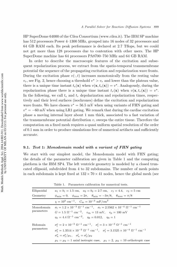
Table 1. Parameters calibration for numerical tests.
Ellipsoidal a1 = b1 = 1.5 cm, a2 = b2 = 2.7 cm, c1 = 4.4, c2 = 5 cm
Geometry φmin = 0, φmax = 2π, θmin = −3π/8, θmax = π/8
χ = 103 cm−1, Cm = 10−3 mF/cm2
Monodomain σl = 1.2 × 10⁻³ Ω−1 cm−1, σt = 2.5562 × 10⁻⁴ Ω−1 cm−1
parameters G = 1.5 Ω−1 cm−2, vth = 13 mV, vp = 100 mV
η1 = 4.4 Ω−1 cm−2, η2 = 0.012, η3 = 1
Bidomain σel
= 2 × 10⁻³ Ω−1 cm−1, σil= 3 × 10⁻³ Ω−1 cm−1
parametersσe
t= 1.3514 × 10⁻³ Ω−1 cm−1, σi
t= 3.1525 × 10⁻⁴ Ω−1 cm−1
σen = σe
t/µ1 , σi
n = σit/µ2
µ1 = µ2 = 1 axial isotropic case, µ1 = 2, µ2 = 10 orthotropic case
Mat
h. M
odel
s M
etho
ds A
ppl.
Sci.
2004
.14:
883-
911.
Dow
nloa
ded
from
ww
w.w
orld
scie
ntif
ic.c
omby
UN
IVE
RSI
TY
OF
MIL
AN
on
03/1
3/13
. For
per
sona
l use
onl
y.

May 31, 2004 15:27 WSPC/103-M3AS 00348
900 P. Colli Franzone & L. F. Pavarino
0.02.04.06.08.0
10.012.014.016.018.020.022.024.026.028.030.032.034.036.038.040.042.044.046.048.050.052.054.056.058.060.062.064.066.068.070.072.074.076.0
.
Fig. 5. Test 1: Isochrones of the depolarization time drawn every 2 msec; anterior (top left),lateral (top center), posterior (top right) epicardial view, meridian section (bottom left), transversesection (bottom right). Values are in msec.
Sec. 6) varies from 264 × 141 × 41 nodes in the smaller case with 4 subdomains
(1.526.184 unknowns) to 1056 × 281 × 41 nodes in the larger case with 32 subdo-
mains (12.166.176 unknowns). We simulated the depolarization of the ventricular
volume after four stimuli of 250 mA/cm3 have been applied for 1 msec on small
areas (five mesh points in each direction) of the epicardium. The model is run for
400 time steps of 0.2 msec each. At each time step, we compute the potential v, the
recovery variable w and the depolarization time of the activated nodes.
In Fig. 5, we plotted the isochrone lines of the depolarization time on three
portions of the epicardial surface (anterior, lateral and posterior), showing the
propagation and merging of the excitation fronts originating at each of the four
stimulation sites, and on two transversal sections showing the intramural propaga-
tion of the fronts.
The timings results reported in Table 2 show that the assembling times
for the stiffness and mass matrices (fourth column) are reasonably small. The
Mat
h. M
odel
s M
etho
ds A
ppl.
Sci.
2004
.14:
883-
911.
Dow
nloa
ded
from
ww
w.w
orld
scie
ntif
ic.c
omby
UN
IVE
RSI
TY
OF
MIL
AN
on
03/1
3/13
. For
per
sona
l use
onl
y.

May 31, 2004 15:27 WSPC/103-M3AS 00348
A Parallel Solver for Reaction–Diffusion Systems 901
Table 2. Test 1: Monodomain with a variant of FHN model. De-
polarization of full ventricle: 4 stimuli applied to the epicardialsurface, 400 time steps of 0.2 msec each, computation of v, w andisochrones. tA = assembly timing, it. = average number of PCGiterations at each time step, time = average CPU timing of eachtime step.
unknowns tA it. time
# proc. mesh (nodes) (s) (s)
4 = 2 · 2 · 1 264 × 141 × 41 1.526.184 10 10 3.5
9 = 3 · 3 · 1 396 × 211 × 41 3.425.796 11.2 12 5.9
16 = 4 · 4 · 1 528 × 281 × 41 6.083.088 11.1 14 8.6
32 = 8 · 4 · 1 1056 × 281 × 41 12.166.176 12.1 21 15
average number of PCG iterations per time step (fifth column) and the average
timing per time step (last column) show the lack of scalability of the one-level
block-Jacobi preconditioner, but for these numbers of processors these values are
quite reasonable.
9.2. Test 2: Monodomain-LR1 model
We consider next the Monodomain equation with LR1 ionic model, simulating
now the initial depolarization of some ellipsoidal blocks after one stimulus of
250 mA/cm3 has been applied for 1 msec on a small area (5 mesh points in each
direction) of the epicardium. The blocks are chosen in increasing sizes so as to keep
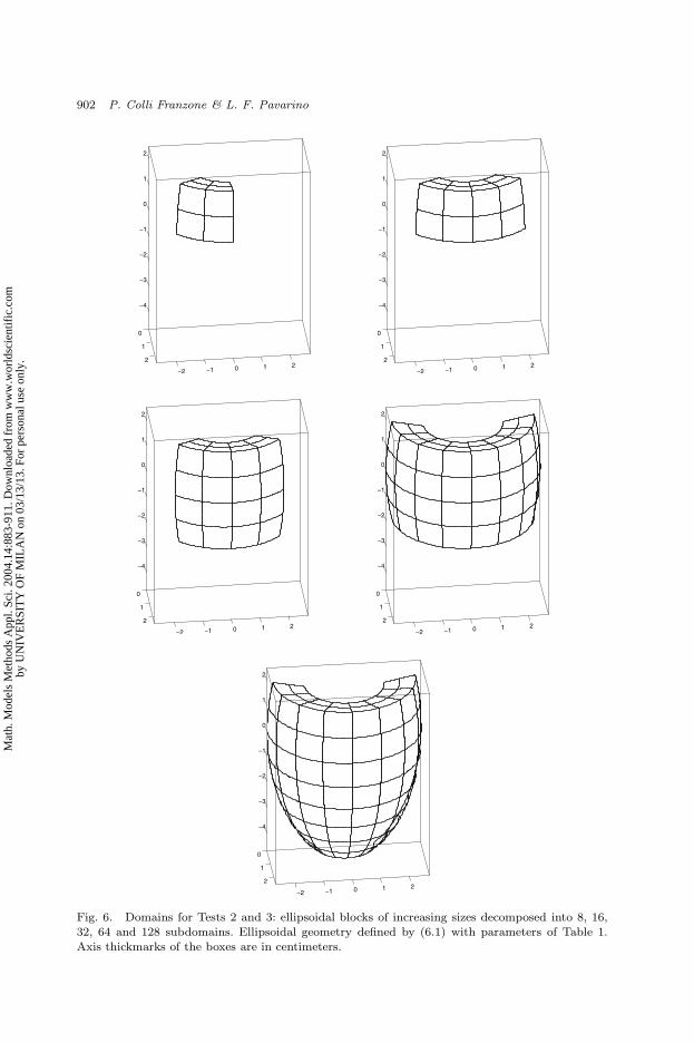
the number of mesh points per subdomain (processor) constant. As shown in Fig. 6,
the domain varies from the smaller block with 8 subdomains to half ventricle with
128 subdomains. We fixed the local mesh in each subdomain to be of 75 × 75× 50
nodes (281.750 unknowns), hence varying the global number of unknowns of the
linear system from 2.25 × 10⁶ in the smaller case with 8 subdomains on a global
mesh of 150 × 150 × 100 nodes to 3.6 × 10⁷ in the larger case with 128 subdo-
mains on a global mesh of 600 × 600 × 100 nodes. The model is run for 30 time
steps of 0.05 msec each. At each time step, we compute the potential v, the gating
and concentration variables w1, . . . , w7 and the depolarization time. The computing
platform is the IBM SP4.
The results are reported in Table 3. The assembling time, average number of
PCG iterations per time step and the average timing per time step (last three
columns) are reasonably small and actually smaller than the results of Test 1, due
to the smaller problem size per processor and time-step size. Up to 64 processors,
the algorithm seems practically scalable, and even for 128 processors, the number of
PCG iterations grows to just 8. The time spent by the solver in the LR1 membrane
routine is about 1.4 sec. per time step and is independent of the global mesh size,
since this routine is completely parallel (it depends of course on the local mesh size,
here kept fixed). Therefore, its relative importance decreases as the problem size
(and processor count) increases.
Mat
h. M
odel
s M
etho
ds A
ppl.
Sci.
2004
.14:
883-
911.
Dow
nloa
ded
from
ww
w.w
orld
scie
ntif
ic.c
omby
UN
IVE
RSI
TY
OF
MIL
AN
on
03/1
3/13
. For
per
sona
l use
onl
y.
May 31, 2004 15:27 WSPC/103-M3AS 00348
902 P. Colli Franzone & L. F. Pavarino
0
1
2
−2 −1 0 1 2
−4
−3
−2
−1
0
1
2
0
1
2
−2 −1 0 1 2
−4
−3
−2
−1
0
1
2
0
1
2
−2 −1 0 1 2
−4
−3
−2
−1
0
1
2
0
1
2
−2 −1 0 1 2
−4
−3
−2
−1
0
1
2
0
1
2
−2 −1 0 1 2
−4
−3
−2
−1
0
1
2
Fig. 6. Domains for Tests 2 and 3: ellipsoidal blocks of increasing sizes decomposed into 8, 16,32, 64 and 128 subdomains. Ellipsoidal geometry defined by (6.1) with parameters of Table 1.Axis thickmarks of the boxes are in centimeters.
Mat
h. M
odel
s M
etho
ds A
ppl.
Sci.
2004
.14:
883-
911.
Dow
nloa
ded
from
ww
w.w
orld
scie
ntif
ic.c
omby
UN
IVE
RSI
TY
OF
MIL
AN
on
03/1
3/13
. For
per
sona
l use
onl
y.
May 31, 2004 15:27 WSPC/103-M3AS 00348
A Parallel Solver for Reaction–Diffusion Systems 903
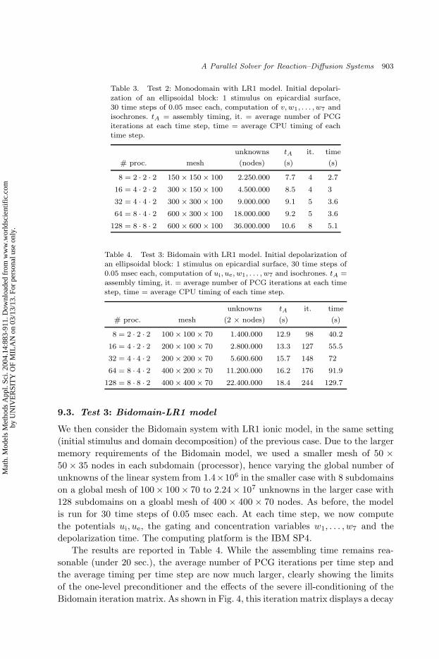
Table 3. Test 2: Monodomain with LR1 model. Initial depolari-
zation of an ellipsoidal block: 1 stimulus on epicardial surface,30 time steps of 0.05 msec each, computation of v, w1, . . . , w7 andisochrones. tA = assembly timing, it. = average number of PCGiterations at each time step, time = average CPU timing of eachtime step.
unknowns tA it. time
# proc. mesh (nodes) (s) (s)
8 = 2 · 2 · 2 150 × 150 × 100 2.250.000 7.7 4 2.7
16 = 4 · 2 · 2 300 × 150 × 100 4.500.000 8.5 4 3
32 = 4 · 4 · 2 300 × 300 × 100 9.000.000 9.1 5 3.6
64 = 8 · 4 · 2 600 × 300 × 100 18.000.000 9.2 5 3.6
128 = 8 · 8 · 2 600 × 600 × 100 36.000.000 10.6 8 5.1
Table 4. Test 3: Bidomain with LR1 model. Initial depolarization ofan ellipsoidal block: 1 stimulus on epicardial surface, 30 time steps of0.05 msec each, computation of ui, ue, w1, . . . , w7 and isochrones. tA =assembly timing, it. = average number of PCG iterations at each timestep, time = average CPU timing of each time step.
unknowns tA it. time
# proc. mesh (2 × nodes) (s) (s)
8 = 2 · 2 · 2 100 × 100 × 70 1.400.000 12.9 98 40.2
16 = 4 · 2 · 2 200 × 100 × 70 2.800.000 13.3 127 55.5
32 = 4 · 4 · 2 200 × 200 × 70 5.600.600 15.7 148 72
64 = 8 · 4 · 2 400 × 200 × 70 11.200.000 16.2 176 91.9
128 = 8 · 8 · 2 400 × 400 × 70 22.400.000 18.4 244 129.7
9.3. Test 3: Bidomain-LR1 model
We then consider the Bidomain system with LR1 ionic model, in the same setting
(initial stimulus and domain decomposition) of the previous case. Due to the larger
memory requirements of the Bidomain model, we used a smaller mesh of 50 ×
50 × 35 nodes in each subdomain (processor), hence varying the global number of
unknowns of the linear system from 1.4×10⁶ in the smaller case with 8 subdomains
on a global mesh of 100× 100× 70 to 2.24× 10⁷ unknowns in the larger case with
128 subdomains on a gloabl mesh of 400 × 400 × 70 nodes. As before, the model
is run for 30 time steps of 0.05 msec each. At each time step, we now compute
the potentials ui, ue, the gating and concentration variables w1, . . . , w7 and the
depolarization time. The computing platform is the IBM SP4.
The results are reported in Table 4. While the assembling time remains rea-
sonable (under 20 sec.), the average number of PCG iterations per time step and
the average timing per time step are now much larger, clearly showing the limits
of the one-level preconditioner and the effects of the severe ill-conditioning of the
Bidomain iteration matrix. As shown in Fig. 4, this iteration matrix displays a decay
Mat
h. M
odel
s M
etho
ds A
ppl.
Sci.
2004
.14:
883-
911.
Dow
nloa
ded
from
ww
w.w
orld
scie
ntif
ic.c
omby
UN
IVE
RSI
TY
OF
MIL
AN
on
03/1
3/13
. For
per
sona
l use
onl
y.

May 31, 2004 15:27 WSPC/103-M3AS 00348
904 P. Colli Franzone & L. F. Pavarino
of the smallest eigenvalues similar to the stiffness matrix related to the elliptic
operator with homogeneous Neumann boundary conditions. Therefore, we have
applied the same solver to the linear system associated with the elliptic Neumann
problem related to the tensor Di +De, appearing as the algebraic part in the DAE
formulation (6.6). The results show that the iteration counts are of the same order
as those of Table 4. Hence, the loss of efficiency of our Bidomain solver is not due
to the doubling of the unknown size and is also present in the DAE formulation
where the algebraic system is half the size of the Bidomain system.
The time spent by the solver in the LR1 membrane routine is about 0.45 sec.
per time step, independently of the global mesh size; the reduction with respect to
the Monodomain case is due to the reduced local problem size.
9.4. Test 4: Full cardiac cycle with Bidomain-LR1 model
Knowledge of the rules that govern the full cardiac cycle, including excitation and
repolarization processes, is a necessary prerequisite for understanding and inter-
preting abnormal sequences that occur in conduction disturbances, such as cardiac
arrhythmias. However, while the excitation phase has been studied extensively,
both experimentally and numerically, the repolarization phase remains incompletely
understood; see Gotoh et al.,22 Cates and Pollard.10 We now turn our attention to
the simulation of the full cardiac cycle in a slab of cardiac tissue of size 2 ·2 ·0.5 cm3,
discretized with a fine mesh of 201 × 201 × 51 nodes. We use the Bidomain-LR1
model. The fibers rotate intramurally linearly with depth for a total amount of 90,
i.e. α0 = 0.5 in (6.2). In this simulation, we assume a full orthotropic anisotropy
with conductivity coefficients given in Table 1, an(x) = ex sinα(r) − ey cos
α(r) and at = ez. The excitation process is started by applying a stimulus of
250 mA/cm3 for 1 msec on a small area (3 mesh points in each direction) at a
vertex of the slab.
0 100 200 300 40010
−2
10−1
100
101
MSEC.
TIM
E S
TE
P S
IZE
(a)
0 100 200 300 40080
140
200
260
MSEC.
ITE
RA
TIO
NS
(b)
Fig. 7. Test 4: Full cardiac cycle with Bidomain model and LR1 gating. Time-step size in msec.on a semilogarithmic scale (a), (b) PCG iterations at each time step, both as a function of time.
Mat
h. M
odel
s M
etho
ds A
ppl.
Sci.
2004
.14:
883-
911.
Dow
nloa
ded
from
ww
w.w
orld
scie
ntif
ic.c
omby
UN
IVE
RSI
TY
OF
MIL
AN
on
03/1
3/13
. For
per
sona
l use
onl
y.
May 31, 2004 15:27 WSPC/103-M3AS 00348
A Parallel Solver for Reaction–Diffusion Systems 905
Studies of the full cardiac cycle require much longer simulation time intervals,
estimated by adding to the action potential duration (APD), which in the original
LR1 model is more than 400 msec, the total excitation time related to the size of
the cardiac volume. We scaled the slow inward current Isi of the LR1 model by a
factor 2/3, thereby reducing the action potential duration to about 280 msec. Since
the excitation of the entire slab in this test requires about 80 msec, the time interval
for simulating the cardiac cycle is on the order of 400 msec. The adaptive time-
stepping algorithm automatically adapts the time-step size in the different phases
of the simulation. As shown in Fig. 7(a), the initial small time step of 0.05 msec,
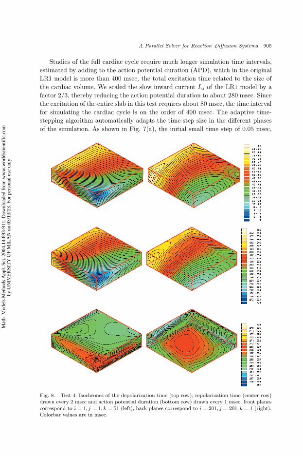
Fig. 8. Test 4: Isochrones of the depolarization time (top row), repolarization time (center row)drawn every 2 msec and action potential duration (bottom row) drawn every 1 msec; front planescorrespond to i = 1, j = 1, k = 51 (left), back planes correspond to i = 201, j = 201, k = 1 (right).Colorbar values are in msec.
Mat
h. M
odel
s M
etho
ds A
ppl.
Sci.
2004
.14:
883-
911.
Dow
nloa
ded
from
ww
w.w
orld
scie
ntif
ic.c
omby
UN
IVE
RSI
TY
OF
MIL
AN
on
03/1
3/13
. For
per
sona
l use
onl
y.
May 31, 2004 15:27 WSPC/103-M3AS 00348
906 P. Colli Franzone & L. F. Pavarino
needed while the steep depolarization front propagates throughout the domain, is
increased to about 0.62 msec in the plateau phase, then decreased to 0.31 and
0.15 msec in the repolarization phase, and finally increased to the maximum size
allowed of 6 msec when most of the tissue has returned to rest. Corresponding to
these phases, the number of PCG iterations of the linear solver change considerably
0 400−25
0
25
1
msec.
mV
0 400
2
msec.
0 400
3
msec.
0 400
4
msec.
−25
0
25
5
mV
6 7 8
−25
0
25
9
mV
10 11 12
−25
0
25
13
mV
14 15 16
S
1 2 3 4
5 6 7 8
9 10 11 12
13 14 15 16
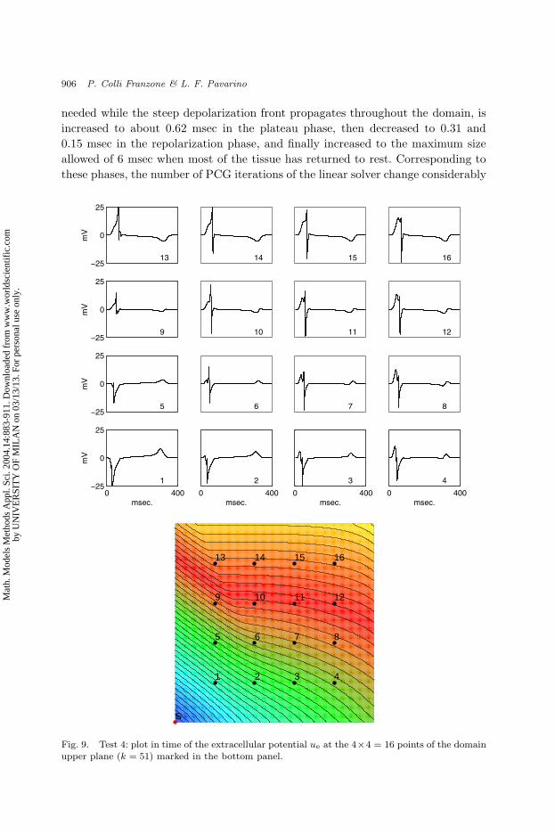
Fig. 9. Test 4: plot in time of the extracellular potential ue at the 4×4 = 16 points of the domainupper plane (k = 51) marked in the bottom panel.
Mat
h. M
odel
s M
etho
ds A
ppl.
Sci.
2004
.14:
883-
911.
Dow
nloa
ded
from
ww
w.w
orld
scie
ntif
ic.c
omby
UN
IVE
RSI
TY
OF
MIL
AN
on
03/1
3/13
. For
per
sona
l use
onl
y.
May 31, 2004 15:27 WSPC/103-M3AS 00348
A Parallel Solver for Reaction–Diffusion Systems 907
(a) (b)
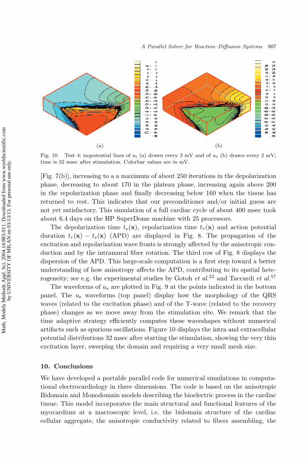
Fig. 10. Test 4: isopotential lines of ui (a) drawn every 3 mV and of ue (b) drawn every 2 mV;time is 32 msec after stimulation. Colorbar values are in mV.
[Fig. 7(b)], increasing to a a maximum of about 250 iterations in the depolarization
phase, decreasing to about 170 in the plateau phase, increasing again above 200
in the repolarization phase and finally decreasing below 160 when the tissue has
returned to rest. This indicates that our preconditioner and/or initial guess are
not yet satisfactory. This simulation of a full cardiac cycle of about 400 msec took
about 6.4 days on the HP SuperDome machine with 25 processors.
The depolarization time te(x), repolarization time tr(x) and action potential
duration tr(x) − te(x) (APD) are displayed in Fig. 8. The propagation of the
excitation and repolarization wave fronts is strongly affected by the anisotropic con-
duction and by the intramural fiber rotation. The third row of Fig. 8 displays the
dispersion of the APD. This large-scale computation is a first step toward a better
understanding of how anisotropy affects the APD, contributing to its spatial hete-
rogeneity; see e.g. the experimental studies by Gotoh et al.22 and Taccardi et al.
57
The waveforms of ue are plotted in Fig. 9 at the points indicated in the bottom
panel. The ue waveforms (top panel) display how the morphology of the QRS
waves (related to the excitation phase) and of the T-wave (related to the recovery
phase) changes as we move away from the stimulation site. We remark that the
time adaptive strategy efficiently computes these waveshapes without numerical
artifacts such as spurious oscillations. Figure 10 displays the intra and extracellular
potential distributions 32 msec after starting the stimulation, showing the very thin
excitation layer, sweeping the domain and requiring a very small mesh size.
10. Conclusions
We have developed a portable parallel code for numerical simulations in computa-
tional electrocardiology in three dimensions. The code is based on the anisotropic
Bidomain and Monodomain models describing the bioelectric process in the cardiac
tissue. This model incorporates the main structural and functional features of the
myocardium at a macroscopic level, i.e. the bidomain structure of the cardiac
cellular aggregate, the anisotropic conductivity related to fibers assembling, the
Mat
h. M
odel
s M
etho
ds A
ppl.
Sci.
2004
.14:
883-
911.
Dow
nloa
ded
from
ww
w.w
orld
scie
ntif
ic.c
omby
UN
IVE
RSI
TY
OF
MIL
AN
on
03/1
3/13
. For
per
sona
l use
onl
y.

May 31, 2004 15:27 WSPC/103-M3AS 00348
908 P. Colli Franzone & L. F. Pavarino
fiber rotation through the ventricular wall thickness, the laminar structure of the
fiber architecture and the LR1 cellular membrane model, one of the most used in
the literature. The FORTRAN code is based on structured isoparametric Q1 finite
elements in space and a semi-implicit adaptive method in time. Parallelization and
portability are based on the PETSc parallel library. Large-scale simulations with up
to O(107) unknowns have been run on IBM SP4 and HP SuperDome parallel com-
puters. We expect to be able to run simulations with O(108) unknowns on machines
with O(103) processors. These simulations have shown that our numerical methods
have a good performance when applied to the Monodomain model, even for a full
left ventricular domain, while they need improvement in the Bidomain case, where
a full heartbeat could be simulated only in a relatively small 3D block of tissue. The
loss of efficiency in the Bidomain case is mostly related to the solution of the linear
system at each time step and is shared by both the ui,ue and the v,ue formulations.
This is not only due to the doubling of the unknowns but can be attributed to the
worst conditioning of the iteration matrix and to our preconditioning technique.
On the other hand, it is well established by the agreement between experimental
and simulated data that the bidomain structure cannot be neglected in modern
simulation studies. Therefore, work is under way to develop more efficient elliptic
solvers based on two-level domain decomposition methods and more efficient time
advancement methods.
References
1. Special issue on Fibrillation in normal ventricular myocardium, Chaos 8 (1) (1998).2. Special issue on Mapping and control of complex cardiac arrhythmias, Chaos 12 (3)
(2002).3. Special issue on From excitable media to virtual cardiac tissue, Chaos Solit. Frac. 13
(8) (2002).4. L. Ambrosio, P. Colli Franzone and G. Savare, On the asymptotic behaviour of
anisotropic energies arising in the cardiac bidomain model, Interfaces Free Bound.
2 (2000) 213–266.5. O. M. Ascher, S. J. Ruuth and B. T. R. Wetton, Implicit-explicit methods for
time-dependent partial differential equations, SIAM J. Numer. Anal. 32 (1995)797–823.
6. S. Balay, K. Buschelman, W. D. Gropp, D. Kaushik, M. Knepley, L. Curfman McInnes,B. F. Smith and H. Zhang, PETSc Users Manual. Tech. Rep. ANL-95/11 — Revision2.1.5, Argonne National Laboratory (2002).
7. S. Balay, K. Buschelman, W. D. Gropp, D. Kaushik, M. Knepley, L. Curfman McInnes,B. F. Smith and H. Zhang, PETSc home page. http://www.mcs.anl.gov/petsc, 2001.
8. G. Bellettini, P. Colli Franzone and M. Paolini, Convergence of front propagation foranisotropic bistable reaction–diffusion equations, Asymp. Anal. 15 (1997) 325–358.
9. N. F. Britton, Reaction–diffusion Equations and Their Applications to Biology
(Academic Press, 1986).10. A. W. Cates and A. E. Pollard, A model study of intramural dispersion of action
potential duration in the canine pulmonary conus, Ann. Biomed. Engrg. 26 (1998)567–576.
11. E. M. Cherry, H. S. Greenside and C. S. Henriquez, A space-time adaptive methodfor simulating complex cardiac dynamics, Phys. Rev. Lett. 84 (2000) 1343–1346.
Mat
h. M
odel
s M
etho
ds A
ppl.
Sci.
2004
.14:
883-
911.
Dow
nloa
ded
from
ww
w.w
orld
scie
ntif
ic.c
omby
UN
IVE
RSI
TY
OF
MIL
AN
on
03/1
3/13
. For
per
sona
l use
onl
y.
May 31, 2004 15:27 WSPC/103-M3AS 00348
A Parallel Solver for Reaction–Diffusion Systems 909
12. P. Colli Franzone and L. Guerri, Spread of excitation in 3-D models of the anisotropiccardiac tissue, I: Validation of the eikonal approach, Math. Biosci. 113 (1993)145–209.
13. P. Colli Franzone, L. Guerri, M. Pennacchio and B. Taccardi, Spread of excitationin 3-D models of the anisotropic cardiac tissue, II: Effects of fiber architecture andventricular geometry, Math. Biosci. 147 (1998) 131–171.
14. P. Colli Franzone, L. Guerri, M. Pennacchio and B. Taccardi, Spread of excitation in3-D models of the anisotropic cardiac tissue. III: Effects of ventricular geometry andfiber structure on the potential distribution, Math. Biosci. 151 (1998) 51–98.
15. P. Colli Franzone, L. Guerri, M. Pennacchio and B. Taccardi, Anisotropic mechanismsfor multiphasic unipolar electrograms. Simulation studies and experimental record-ings, Ann. Biomed. Engrg. 28 (2000) 1–17.
16. P. Colli Franzone, M. Pennacchio and L. Guerri, Accurate computation of electro-grams in the left ventricular wall, Math. Mod. Meth. Appl. Sci. 10 (2000) 507–538.
17. P. Colli Franzone and G. Savare, Degenerate evolution systems modeling the cardiacelectric field at micro and macroscopic level, in Evolution Equations, Semigroups and
Functional Analysis, eds. A. Lorenzi and B. Ruf (Birkhauser, 2002), pp. 49–78.18. J. W. Demmel, M. T. Heath and H. A. van der Vorst, Parallel numerical linear algebra,
Acta Numer. (1993) 111–197.19. I. R. Efimov, B. Ermentrout, D. T. Huang and G. Salama, Activation and repolari-
zation patterns are governed by different structural characteristics of ventricularmyocardium: experimental study with voltage-sensitive dyes and numerical simula-tions, J. Cardiovasc. Electrophysiol. 7 (1996) 512–530.
20. F. H. Fenton and A. Karma, Vortex dynamics in three-dimensional continuousmyocardium with fiber rotation: filament instability and fibrillation, Chaos 8 (1998)20–47.
21. A. Garfinkel, Y.-H. Kim, O. Voroshilovsky, Z. Qu, J. R. Kil, M.-H. Lee, H. S.Karagueuzian, J. N. Weiss and P.-S. Chen, Preventing ventricular fibrillation by flat-tening cardiac restitution, Proc. Nat. Acad. Sci. USA 97 (2000) 6061–6066.
22. M. Gotoh et al., Anisotropic repolarization in ventricular tissue, Amer. J. Physiol.
41 (1997) 107–113.23. C. S. Henriquez, Simulating the electrical behavior of cardiac tissue using the bido-
main model, Crit. Rev. Biomed. Engrg. 21 (1993) 1–77.24. C. S. Henriquez, A. L. Muzikant and C. K. Smoak, Anisotropy, fiber curvature,
and bath loading effects on activation in thin and thick cardiac tissue preparations:Simulations in a three-dimensional bidomain model, J. Cardiovasc. Electrophysiol. 7
(1996) 424–444.25. A. L. Hodgkin and A. F. Huxley, A quantitative description of membrane current
and its application to conduction and excitation in nerve, J. Physiol. 117 (1952)500–544.
26. N. Hooke, Efficient simulation of action potential propagation in a bidomain. Ph.D.Thesis, Duke Univ., Dept. of Comput. Sci., 1992.
27. N. Hooke, C. S. Henriquez, P. Lanzkrom and D. Rose, Linear algebraic transforma-tions of the bidomain equations: implications for numerical methods, Math. Biosci.
120 (1994) 127–145.28. J. P. Keener, An eikonal-curvature equation for the action potential propagation in
myocardium, J. Math. Biol. 29 (1991) 629–651.29. J. P. Keener and K. Bogar, A numerical method for the solution of the bidomain
equations in cardiac tissue, Chaos 8 (1998) 234–241.30. J. P. Keener and J. Sneyd, Mathematical Physiology (Springer-Verlag, 1998).
Mat
h. M
odel
s M
etho
ds A
ppl.
Sci.
2004
.14:
883-
911.
Dow
nloa
ded
from
ww
w.w
orld
scie
ntif
ic.c
omby
UN
IVE
RSI
TY
OF
MIL
AN
on
03/1
3/13
. For
per
sona
l use
onl
y.
May 31, 2004 15:27 WSPC/103-M3AS 00348
910 P. Colli Franzone & L. F. Pavarino
31. I. J. LeGrice, B. H. Smaill, L. Z. Chai, S. G. Edgar, J. B. Gavin and P. J. Hunter,Laminar structure of the heart: ventricular myocyte arrangement and connectivetissue architecture in the dog, Am. J. Physiol. (Heart Circ. Physiol.) 269 (1995)H571–H582.
32. C. Luo and Y. Rudy, A model of the ventricular cardiac action potential: depolariza-tion, repolarization, and their interaction, Circ. Res. 68 (1991) 1501–1526.
33. P. K. Moore, An adaptive finite element method for parabolic differential systems:some algorithmic considerations in solving in three space dimensions, SIAM J. Sci.
Comput. 21 (2000) 1567–1586.34. A. L. Muzikant, E. W. Hsu, P. D. Wolf and C. S. Henriquez, Region specific modeling
of cardiac muscle: comparison of simulated and experimental potentials, Ann. Biomed.
Engrg. 30 (2002) 867–883.35. J. S. Neu and W. Krassowska, Homogenization of syncytial tissues, Crit. Rev. Biom.
Engrg. 21 (1993) 137–199.36. N. F. Otani, Computer modeling in cardiac electrophysiology, J. Comput. Phys. 161
(2000) 21–34.37. A. V. Panfilov, Spiral breakup as a model of ventricular fibrillation, Chaos 8 (1998)
57–64.38. A. V. Panfilov and A. V. Holden, Computational Biology of the Heart (Wiley, 1997).39. M. Pennacchio, The mortar finite element method for the cardiac “bidomain” model
of extracellular potential, J. Sci. Comp., to appear.40. M. Pennacchio and V. Simoncini, Efficient algebraic solution of reaction–diffusion
systems for the cardiac excitation process, J. Comput. Appl. Math. 145 (2002) 49–70.41. C. S. Peskin, Fiber architecture of the left ventricular wall: an asymptotic analysis,
Comm. Pure Appl. Math. 42 (1989) 79–113.42. J. Pormann, A Simulation System for the Bidomain Equations, Ph.D. Thesis, Duke
Univ., Dept. of Electr. Comput. Eng., 1999.43. Z. Qu and A. Garfinkel, An advanced algorithm for solving partial differential equation
in cardiac conduction, IEEE Trans. Biomed. Engrg. 46 (1997) 1166–1168.44. W. Quan, S. J. Evans and H. M. Hastings, Efficient integration of a realistic two-
dimensional cardiac tissue model by domain decomposition, IEEE Trans. Biomed.
Engrg. 45 (1998) 372–385.45. A. Quarteroni and A. Valli, Numerical Approximation of Partial Differential Equa-
tions (Springer-Verlag, 1994).46. W. J. Rappel, Filament instability and rotational tissue anisotropy: A numerical study
using detailed cardiac models, Chaos 11 (2001) 71-80.47. J. M. Rogers and A. D. McCulloch, A collocation-Galerkin finite element model of
cardiac action potential propagation, IEEE Trans. Biomed. Engrg. 41 (1994) 743–757.48. B. J. Roth, Action potential propagation in a thick strand of cardiac muscle, Circ.
Res. 68 (1991) 162–173.49. B. J. Roth, How the anisotropy of the intracellular and extracellular conductivities
influence stimulation of cardiac muscle, J. Math. Biol. 30 (1992) 633–646.50. H. I. Saleheen and K. T. Ng, A new three-dimensional finite-difference bidomain
formulation for inhomogeneous anisotropic cardiac tissues, IEEE Trans. Biomed.
Engrg. 45 (1998) 15–25.51. S. Sanfelici, Convergence of the Galerkin approximation of a degenerate evolution
problem in electrocardiology, Numer. Meth. Part. Diff. Eq. 18 (2002) 218–240.52. B. F. Smith, P. Bjørstad and W. D. Gropp, Domain Decomposition: Parallel Multi-
level Methods for Elliptic Partial Differential Equations (Cambridge University Press,1996).
Mat
h. M
odel
s M
etho
ds A
ppl.
Sci.
2004
.14:
883-
911.
Dow
nloa
ded
from
ww
w.w
orld
scie
ntif
ic.c
omby
UN
IVE
RSI
TY
OF
MIL
AN
on
03/1
3/13
. For
per
sona
l use
onl
y.
May 31, 2004 15:27 WSPC/103-M3AS 00348
A Parallel Solver for Reaction–Diffusion Systems 911
53. J. Smoller, Shock Waves and Reaction–Diffusion Equations (Springer-Verlag, 1994),2nd edn.
54. D. Streeter, Gross morphology and fiber geometry in the heart, in Handbook of
Physiology, ed. R. M. Berne (Williams & Wilkins, 1979), Vol. 1, Sec. 2, pp. 61–112.55. J. Sudnes, G. T. Lines and A. Tveito, Efficient solution of ordinary differential
equations modeling electrical activity in cardiac cells, Math. Biosci. 172 (2003)55–72.
56. B. Taccardi, E. Macchi, R. L. Lux, P. R. Ershler, S. Spaggiari, S. Baruffi andY. Vyhmeister, Effect of myocardial fiber direction on epicardial potentials, Circula-
tion 90 (1994) 3076–3090.57. B. Taccardi, B. Punske. F. Helie, R. MacLeod, R. Lux, P. Ershler, T. Dustman and
Y. Vyhmeister, Epicardial recovery sequences and excitation recovery intervals duringpaced beats. Role of myocardial architecture, PACE 22 (1999) 833.
58. N. Trayanova, J. Eason and F. Aguel, Computer simulations of cardiac defibrillation:a look inside the heart, Comput. Visual. Sci. 4 (2002) 259–270.
59. M. Veneroni, Il modello di Hodgkin–Huxley per la propagazione del campo elettricocardiaco, IMATI Tech. Rep., 2003, to appear.
60. B. Victorri, A. Vinet, F. A. Roberge and J. P. Drouhard, Numerical integration inthe reconstruction of cardiac action potentials using Hodgkin–Huxley type models,Comp. Biomed. Res. 18 (1985) 10–23.
61. E. J. Vigmond, F. Aguel and N. A. Trayanova, Computational techniques for solvingthe bidomain equations in three dimensions, IEEE Trans. Biomed. Engrg. 49 (2002)1260–1269.
62. A. T. Winfree, Stable particle-like solutions to the nonlinear wave equations ofthree-dimensional excitable media, SIAM Rev. 32 (1990) 1–53.
63. A. T. Winfree, Electrical turbulence in three-dimensional heart muscle, Science 266
(1994) 1003–1006.64. H. Yu, Solving parabolic problems with different time steps in different regions in space
based on domain decomposition methods, Appl. Numer. Math. 30 (1999) 475–491.65. H. Yu, A local space-time adaptive scheme in solving two-dimensional parabolic
problems based on domain decomposition methods, SIAM J. Sci. Comput. 23 (2001)304–322.
66. D. Zipes and J. Jalife, Cardiac Electrophysiology (W. B. Sauders Co., 2000).
Mat
h. M
odel
s M
etho
ds A
ppl.
Sci.
2004
.14:
883-
911.
Dow
nloa
ded
from
ww
w.w
orld
scie
ntif
ic.c
omby
UN
IVE
RSI
TY
OF
MIL
AN
on
03/1
3/13
. For
per
sona
l use
onl
y.