APPROXIMATION TO THE MEAN CURVE IN THE LCS PROBLEM

CLEMENT DURRINGER!, RAPHAEL HAUSER†!AND HEINRICH MATZINGER ‡!

Abstract. The problem of sequence comparison via optimal alignments occurs naturally in

many areas of applications. The simplest such technique is based on evaluating a score given by the

length of a longest common subsequence divided by the average length of the original sequences. In

this paper we investigate the expected value of this score when the input sequences are random and

their length tends to infinity. The corresponding limit exists but is not known precisely. We derive

a large-deviation, convex analysis and Montecarlo based method to compute a consistent sequence

of upper bounds on the unknown limit.

AMS subject classifications. Primary 05A16, 62F10. Secondary 92E10.

Key words. Longest common subsequence problem, Chvatal-Sanko! constant, Steele conjec-

ture, mean curve, large deviation theory, Montecarlo simulation, convex analysis.

1. Introduction. A naive way of quantifying the similarity of two finite strings

is to compare them character by character and count the number of matching symbols.

For example, the strings T1 = ’nebbiolo’ and T2 = ’nbbiolo’ have only two common

characters under this method of comparison and would not be judged very similar.

The design of more meaningful methods of comparing strings often depends on specific

applications such genetic sequence analysis, speech recognition or file comparison.

A family of sophisticated methods is based on looking at subsequences of the

original strings and their likely descendants under a mutation process based on a

hidden Markov model. The simplest method of this kind is to measure the similarity

between strings by the relative length of a longest common subsequence (LCS) with

respect to the mean of the lengths of the original sequences. A subsequence of a string

!All three authors would like to thank for support through the Sonderforschungsbereich GrantSFB 701 A3 from the German Research Foundation.

†Oxford University Computing Laboratory, Wolfson Building, Parks Road, Oxford, OX1 3QD,United Kingdom, (hauser@comlab.ox.ac.uk). This author was supported through grant GR/S34472from the Engineering and Physical Sciences Research Council of the UK and through grantNAL/00720/G from the Nu"eld Foundation.

‡School of Mathematics, Georgia Institute of Technology, 686 Cherry Street, Atlanta, GA 30332-0160, USA, (matzi@math.gatech.edu).

1

is defined as any string obtained by deleting some of the characters from the original

string and keeping the remaining characters in the same order. For example, the

strings T1 and T2 defined above contain ’nbbiolo’ as a longest common subsequence

and have a similarity score of 93.33% under this method of comparison.

In order to use string comparison algorithms for the detection of sequences that

are closely related to one another, one must be able to tell when a similarity score

is significantly higher than scores that are likely to occur when comparing random

strings. The study of the distribution of scores under random input strings is therefore

of great interest.

In this paper we study the asymptotic expectation of the LCS method. To fix

ideas, let (Xsn)N (s = 1, 2) be two independent sequences of i.i.d. standard Bernoulli

random variables. For all ! = (!1,!2) ! R2+ such that !1 + !2 = 1 let Ln(!) denote

the length of a longest common subsequence of the two strings (Xs1 , Xs

2 , . . . , Xs!2!sn")

(s = 1, 2). Note that Ln(!) is well-defined, but there may be more than one common

subsequence of this length. A simple subadditivity argument shows that the limit

"(!) := limn#$ E[Ln(!)/n] exists. The function ! " "(!) is called the mean curve

of the LCS-problem. This definition has an immediate extension to the case where

r sequences (Xsn)N (s = 1, . . . , r) of i.i.d. random variables Xs

n with distribution µ

in a finite alphabet A are considered. The mean curve is concave and symmetric in

!. Montecarlo simulation methods for the computation of probabilistic lower bounds

on "(!) are readily available through the exploitation of subadditivity. Furthermore,

in the case where r = 2 methods for the computation of both probabilistic and

deterministic upper and lower bounds on the value "(1/2, 1/2)) have been derived in

a number of papers [6, 9, 7, 13, 1, 4, 11, 8].

In this paper we discuss a method for the computation of upper bounds on the

mean curve based on large deviations technology. This extends the upper bound

method derived in [11] for the case "(1/2, 1/2)), r = 2. Our method depends on a

finite measure #m,r that encapsulates information about the probability that random

sequences of given lengths are so-called m-matches, defined by the properties of hav-

2

ing a LCS of length exactly m and by requiring that the last characters of each of

the sequences must be aligned to achieve this score. Our method then boosts any

known information about the score distribution of shorter strings (through partial

knowledge of the measure #m,r) to derive information about the expected LCS scores

of longer r-tuples of random sequences by decomposing the latter into a concatena-

tion of m-matches. In practice the measure #m,r is not known exactly, but it can

be approximated arbitrarily well via simulations. Simulated partial knowledge about

#m,r leads to probabilistic upper bounds qm,"(!) which depend on the number $ of

simulations as well as the parameter m. For any given %, & > 0 one can choose m#

and $$ such that for all m # m# and $ # $$,

P["(!) $ qm,"(!) $ "(!) + &] # 1% %,

that is, qm,"(!) approximates "(!) to precision & at the confidence level 1% %.

The paper is structured as follows. In Section 2 we introduce the basic concepts

of our analysis and prove some of their elementary properties. Section 3 serves to

characterize upper bounds on "(!) via a criterion that is amenable to numerical com-

putations via optimization problems that depend on the parameter m. Furthermore,

the criterion is used to show that the solutions qm(!) of these optimization problems

form a consistent sequence (qm(!))m%N of upper bounds on "(!), in other words,

limm#$ qm(!) = "(!). Practical computations and numerical results are discussed

in Section 4. Our results yield strong numerical evidence that the so-called Steele-

conjecture [15] is likely not true.

2. Basic Concepts and Notation. This section is devoted to building the

main tools we need in the analysis of Sections 3 and 4.

2.1. The General Setup. For convenience we use the shorthand notation Nn :=

{1, . . . , n}. We denote the canonical basis vectors of Rr by e1, . . . , er and write3

e :=!r

s=1 es for the r-vector of ones. Let A be a finite alphabet and µ a proba-

bility measure on A with µmin := mina%A µ(a) > 0. Throughout this paper X ="(X1

n)N, . . . , (Xrn)N#

denotes an independent r-tuple of infinite sequences of i.i.d. ran-

dom variables Xsn with law µ.

2.2. Strings and Subsequences. We write A& :=$

n%N An for the set of

finite strings with characters in A and #x := n for the length of a finite string

x = (x1, . . . , xn) ! A&. If x ! A&&AN and i, j $ #x we write x[i, j] := (xi, . . . , xj) for

the piece of x between indices i and j. We take this to be the empty string if j < i.

Furthermore, if x ! A& we use the shorthand notation x['] := x[1, #x % 1] for the

string that is left after truncating the last character. The set of subsequences of x,

Sub(x) :=%"

x%(1), . . . , x%(k)

#: k ! N, ' : Nk " N#x strictly increasing

&

consists of the strings obtained by deleting some of the characters of x and keeping

the remaining ones in the original order.

2.3. Vectorized Notation. Extending the introduced notation to r-tuples x =

(x1, . . . , xr) of strings, we write #x for the vector (#x1, . . . , #xr), x' for the set

of r-tuples%"

x1['], x2, . . . , xr#, . . . ,"x1, . . . , xr'1, xr[']

#&, and x[i, j] for the r-tuple

"x1[i1, j1], . . . , xr[ir, jr]

#when i, j ! Nr are multi-indices. Finally, we write |i| :=

!s is, and i < j if ir < jr for all r.

2.4. Longest Common Subsequences. The set of common subsequences of

x ! A&r is defined by ComSub(x) :='

s%NrSub(xs), and the length of a longest

common subsequence of x by LCS(x) := max%#y : y ! ComSub(x)

&. The function

x '" LCS(x) can easily be evaluated: define a function incr : Nr0 ( A&r " {0, 1}

by incr(i, x) := ("x1

i1 , . . . , xrir

#, where ( is the Kronecker delta, that is, ( = 1 if all

arguments are defined and equal, and ( = 0 otherwise. Let Score : Nr0 ( A&r " N

4

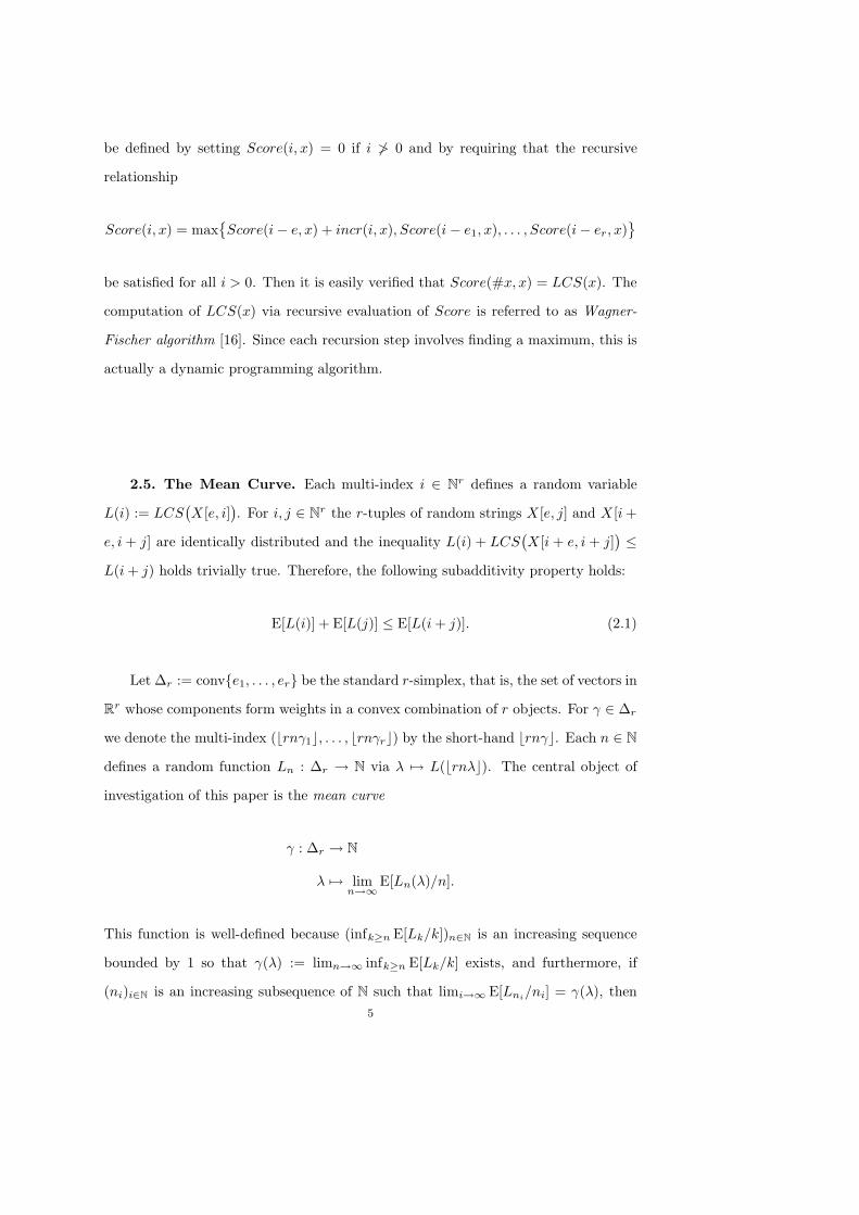
be defined by setting Score(i, x) = 0 if i )> 0 and by requiring that the recursive

relationship

Score(i, x) = max%Score(i% e, x) + incr(i, x), Score(i% e1, x), . . . , Score(i% er, x)

&

be satisfied for all i > 0. Then it is easily verified that Score(#x, x) = LCS(x). The

computation of LCS(x) via recursive evaluation of Score is referred to as Wagner-

Fischer algorithm [16]. Since each recursion step involves finding a maximum, this is

actually a dynamic programming algorithm.

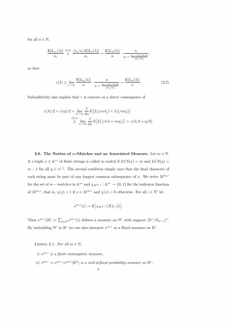
2.5. The Mean Curve. Each multi-index i ! Nr defines a random variable

L(i) := LCS"X [e, i]#. For i, j ! Nr the r-tuples of random strings X [e, j] and X [i +

e, i + j] are identically distributed and the inequality L(i) + LCS"X [i + e, i + j]

#$

L(i + j) holds trivially true. Therefore, the following subadditivity property holds:

E[L(i)] + E[L(j)] $ E[L(i + j)]. (2.1)

Let!r := conv{e1, . . . , er} be the standard r-simplex, that is, the set of vectors in

Rr whose components form weights in a convex combination of r objects. For " ! !r

we denote the multi-index (*rn"1+, . . . , *rn"r+) by the short-hand *rn"+. Each n ! N

defines a random function Ln : !r " N via ! '" L(*rn!+). The central object of

investigation of this paper is the mean curve

" : !r " N

! '" limn#$

E[Ln(!)/n].

This function is well-defined because (infk(n E[Lk/k])n%N is an increasing sequence

bounded by 1 so that "(!) := limn#$ infk(n E[Lk/k] exists, and furthermore, if

(ni)i%N is an increasing subsequence of N such that limi#$ E[Lni/ni] = "(!), then5

for all n ! N,

E[Lni(!)]ni

(2.1)# *ni/n+E[Ln(!)]

ni=

E[Ln(!)]n

· n

n + ni'!ni/n"n!ni/n"

,

so that

"(!) # limi#$

E[Ln(!)]n

· n

n + ni'!ni/n"n!ni/n"

=E[Ln(!)]

n. (2.2)

Subadditivity also implies that " is concave as a direct consequence of

"(!)/2 + "())/2 = limn#$

12n

E(L(*rn!+) + L(*rn)+)

)

(2.1)$ lim

n#$

12n

E(L(*rn!+ rn)+)

)= "(!/2 + )/2).

2.6. The Notion of m-Matches and an Associated Measure. Let m ! N.

A r-tuple x ! A&r of finite strings is called m-match if LCS(x) = m and LCS(y) =

m % 1 for all y ! x[']. The second condition simply says that the final character of

each string must be part of any longest common subsequence of x. We write Mm,r

for the set of m%matches in A&r and *Mm,r : A&r " {0, 1} for the indicator function

of Mm,r, that is, *(x) = 1 if x !Mm,r and *(x) = 0 otherwise. For all i ! Nr let

#m,r(i) := E(*Mm,r (X [e, i])

).

Then #m,r(B) :=!

i%B #m,r(i) defines a measure on Nr with support (N \ Nm'1)r.

By embedding Nr in Rr we can also interpret #m,r as a Borel measure on Rr.

Lemma 2.1. For all m ! N,

i) #m,r is a finite nonnegative measure,

ii) #m,r := #m,r/#m,r(R2) is a well-defined probability measure on Rr,

6

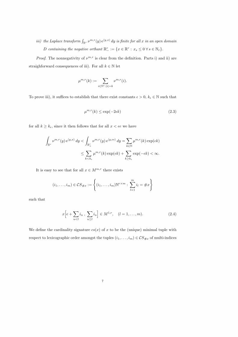
iii) the Laplace transform*

Rr #m,r(y) e)y,x* dy is finite for all x in an open domain

D containing the negative orthant Rr' := {x ! Rr : xs $ 0 , s ! Nr}.

Proof. The nonnegativity of #m,r is clear from the definition. Parts i) and ii) are

straighforward consequences of iii). For all k ! N let

µm,r(k) :=+

i%Nr :|i|=k

#m,r(i).

To prove iii), it su"ces to establish that there exist constants + > 0, k& ! N such that

µm,r(k) $ exp(%2+k) (2.3)

for all k # k&, since it then follows that for all x < +e we have

,

Rr

#m,r(y) e)y,x* dy <

,

Rr+

#m,r(y) e)y,&e* dy =+

k%Nµm,r(k) exp(+k)

$+

k<k!

µm,r(k) exp(+k) ++

k(k!

exp(%+k) <-.

It is easy to see that for all x !Mm,r there exists

(i1, . . . , im) ! CS#x :=

-(i1, . . . , im)Nr+m :

m+

l=1

il = #x

.

such that

x/e ++

u<l

iu ,+

u,l

iu0!M1,r, (l = 1, . . . , m). (2.4)

We define the cardinality signature cs(x) of x to be the (unique) minimal tuple with

respect to lexicographic order amongst the tuples (i1, . . . , im) ! CS#x of multi-indices

7

for which (2.4) holds. We now have

µm,r(k) =+

i%Nr:|i|=k

P [X [e, i] !Mm,r]

=+

i%Nr:|i|=k

+

j%CSi

P(X [e, i] !Mm,r.cs(X [e, i]) = j

)· P [cs(X [e, i]) = j]

$+

i%Nr:|i|=k

+

j=(i1,...,im)%CSi

m1

l=1

2+

a%A,(a)r(1% ,(a))|ir |'r

3· P [cs(X [e, i]) = j]

$ |A|m · (1% ,min)k'mr ,

which implies the required property (2.3).

The measure #m,r is not known explicitly. However, given x ! A&r, we have

x[e, i] ! Mm,r if and only if Score(i, x) = m and Score(i % es, x) = m % 1 for all

s ! Nr. Hence, #m,r can be simulated using the Wagner-Fischer algorithm.

2.7. Parsing Strings into m-Matches. Let x ! A&r be a r-tuple of finite

strings with length i = #x, and let k, m ! N. If LCS(x) # km then there exists at

least one r-tuple - = (-1, . . . ,-r) of increasing functions -s : Nkm " Nis , (s ! Nr)

such that -1(l) = · · · = -r(l) for all l ! Nkm. If we choose - minimal among all

such r-tuples of functions under the partial ordering defined by

- / . 0 -s(l) $ .s(l) , s ! Nr, l ! Nkm,

then x(e,-(m)

), x(-(m)+e,-(2m)

),. . . , x(-((k%1)m)+e,-(km)

), x(-(km)+e, i

)

is a parsing of x into k collated m-matches and a remainder in A&r. Consider the

index set

Ik,mi :=

4(u0, . . . , uk) ! Nr+(k+1) : u0 = 0, uj # me ,j ! Nk,

k+

j=1

uj $ i5.

8

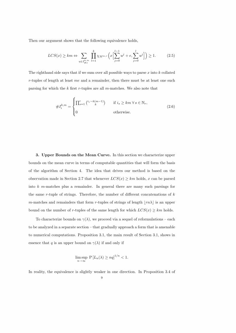
Then our argument shows that the following equivalence holds,

LCS(x) # km0+

u%Ik,m#x

k1

l=1

*Mm,r

6x/ l'1+

j=0

uj + e,l+

j=0

uj07# 1. (2.5)

The righthand side says that if we sum over all possible ways to parse x into k collated

r-tuples of length at least me and a remainder, then there must be at least one such

parsing for which the k first r-tuples are all m-matches. We also note that

#Ik,mi =

899:

99;

<rs=1

"is'k(m'1)k

#if is # km , s ! Nr,

0 otherwise.(2.6)

3. Upper Bounds on the Mean Curve. In this section we characterize upper

bounds on the mean curve in terms of computable quantities that will form the basis

of the algorithm of Section 4. The idea that drives our method is based on the

observation made in Section 2.7 that whenever LCS(x) # km holds, x can be parsed

into k m-matches plus a remainder. In general there are many such parsings for

the same r-tuple of strings. Therefore, the number of di#erent concatenations of k

m-matches and remainders that form r-tuples of strings of length *rn!+ is an upper

bound on the number of r-tuples of the same length for which LCS(x) # km holds.

To characterize bounds on "(!), we proceed via a sequel of reformulations – each

to be analyzed in a separate section – that gradually approach a form that is amenable

to numerical computations. Proposition 3.1, the main result of Section 3.1, shows in

essence that q is an upper bound on "(!) if and only if

lim supn#$

P [Ln(!) # nq]1/n < 1.

In reality, the equivalence is slightly weaker in one direction. In Proposition 3.4 of9

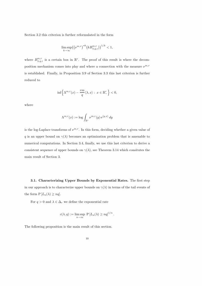
Section 3.2 this criterion is further reformulated in the form

lim supk#$

""#m,r#&k"

kBm,r!,q,#

##1/k< 1,

where Bm,r!,q,# is a certain box in Rr. The proof of this result is where the decom-

position mechanism comes into play and where a connection with the measure #m,r

is established. Finally, in Proposition 3.9 of Section 3.3 this last criterion is further

reduced to

inf4$m,r(x)% rm

q1!, x2 : x ! Rr

'

5< 0,

where

$m,r(x) := log,

Rr

#m,r(y) e)y,x* dy

is the log-Laplace transforms of #m,r. In this form, deciding whether a given value of

q is an upper bound on "(!) becomes an optimization problem that is amenable to

numerical computations. In Section 3.4, finally, we use this last criterion to derive a

consistent sequence of upper bounds on "(!), see Theorem 3.14 which consitutes the

main result of Section 3.

3.1. Characterizing Upper Bounds by Exponential Rates. The first step

in our approach is to characterize upper bounds on "(!) in terms of the tail events of

the form P [Ln(!) # nq].

For q > 0 and ! ! !r we define the exponential rate

c(!, q) := lim supn#$

P [Ln(!) # nq]1/n .

The following proposition is the main result of this section.

10

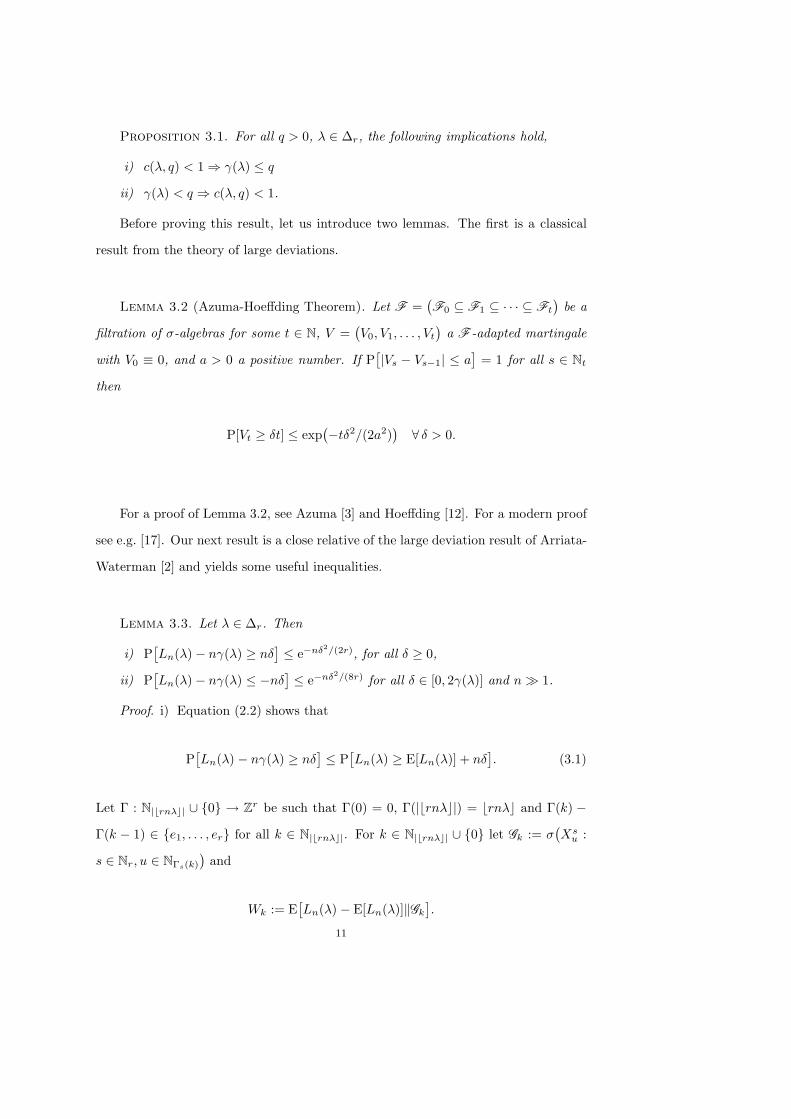
Proposition 3.1. For all q > 0, ! ! !r, the following implications hold,

i) c(!, q) < 13 "(!) $ q

ii) "(!) < q 3 c(!, q) < 1.

Before proving this result, let us introduce two lemmas. The first is a classical

result from the theory of large deviations.

Lemma 3.2 (Azuma-Hoe#ding Theorem). Let F ="F0 4 F1 4 · · · 4 Ft

#be a

filtration of /-algebras for some t ! N, V ="V0, V1, . . . , Vt

#a F -adapted martingale

with V0 5 0, and a > 0 a positive number. If P(|Vs % Vs'1| $ a

)= 1 for all s ! Nt

then

P[Vt # (t] $ exp"%t(2/(2a2)

#, ( > 0.

For a proof of Lemma 3.2, see Azuma [3] and Hoe#ding [12]. For a modern proof

see e.g. [17]. Our next result is a close relative of the large deviation result of Arriata-

Waterman [2] and yields some useful inequalities.

Lemma 3.3. Let ! ! !r. Then

i) P(Ln(!)% n"(!) # n(

)$ e'n'2/(2r), for all ( # 0,

ii) P(Ln(!)% n"(!) $ %n(

)$ e'n'2/(8r) for all ( ! [0, 2"(!)] and n6 1.

Proof. i) Equation (2.2) shows that

P(Ln(!) % n"(!) # n(

)$ P(Ln(!) # E[Ln(!)] + n(

). (3.1)

Let % : N|!rn!"| & {0} " Zr be such that %(0) = 0, %(|*rn!+|) = *rn!+ and %(k) %

%(k % 1) ! {e1, . . . , er} for all k ! N|!rn!"|. For k ! N|!rn!"| & {0} let Gk := /"Xs

u :

s ! Nr, u ! N!s(k)

#and

Wk := E(Ln(!) % E[Ln(!)].Gk

).

11

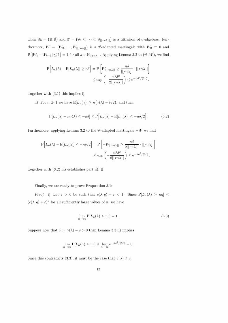
Then G0 = {R, 7} and G ="G0 4 · · · 4 G|!rn!"|

#is a filtration of /-algebras. Fur-

thermore, W ="W0, . . . , W|!rn!"|

#is a G -adapted martingale with W0 5 0 and

P(|Wk%Wk'1| $ 1

)= 1 for all k ! N|!rn!"|. Applying Lemma 3.2 to

"G , W#, we find

P/Ln(!)% E[Ln(!)] # n(

0= P=W|!rn!"| #

n(

|*rn!+| · |*rn!+|>

$ exp?% n2(2

2|*rn!+|

@$ e'n'2/(2r) .

Together with (3.1) this implies i).

ii) For n6 1 we have E[Ln(")] # n""(!)% (/2

#, and then

P[Ln(!) % n"(!) $ %n(] $ P/Ln(!)% E[Ln(!)] $ %n(/2

0. (3.2)

Furthermore, applying Lemma 3.2 to the G -adapted martingale %W we find

P/Ln(!) % E[Ln(!)] $ %n(/2

0= P=%W|!rn!"| #

n(

2|*rn!+| · |*rn!+|>

$ exp?% n2(2

8|*rn!+|

@$ e'n'2/(8r) .

Together with (3.2) his establishes part ii).

Finally, we are ready to prove Proposition 3.1:

Proof. i) Let & > 0 be such that c(!, q) + & < 1. Since P[Ln(!) # nq] $

(c(!, q) + &)n for all su"ciently large values of n, we have

limn#$

P[Ln(!) $ nq] = 1. (3.3)

Suppose now that ( := "(!)% q > 0 then Lemma 3.3 ii) implies

limn#$

P[Ln(") $ nq] $ limn#$

e'n'2/(8r) = 0.

Since this contradicts (3.3), it must be the case that "(!) $ q.

12

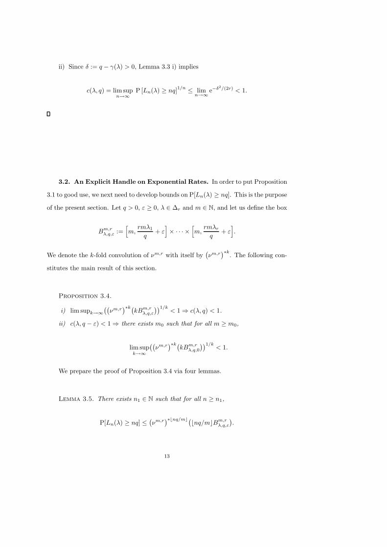
ii) Since ( := q % "(!) > 0, Lemma 3.3 i) implies

c(!, q) = lim supn#$

P [Ln(!) # nq]1/n $ limn#$

e''2/(2r) < 1.

3.2. An Explicit Handle on Exponential Rates. In order to put Proposition

3.1 to good use, we next need to develop bounds on P[Ln(!) # nq]. This is the purpose

of the present section. Let q > 0, & # 0, ! ! !r and m ! N, and let us define the box

Bm,r!,q,# :=

/m,

rm!1

q+ &0( · · ·(

/m,

rm!r

q+ &0.

We denote the k-fold convolution of #m,r with itself by"#m,r#&k. The following con-

stitutes the main result of this section.

Proposition 3.4.

i) lim supk#$""#m,r#&k"

kBm,r!,q,#

##1/k< 13 c(!, q) < 1.

ii) c(!, q % &) < 13 there exists m0 such that for all m # m0,

lim supk#$

""#m,r#&k"

kBm,r!,q,0

##1/k< 1.

We prepare the proof of Proposition 3.4 via four lemmas.

Lemma 3.5. There exists n1 ! N such that for all n # n1,

P[Ln(!) # nq] $"#m,r#&!nq/m""*nq/m+Bm,r

!,q,#

#.

13

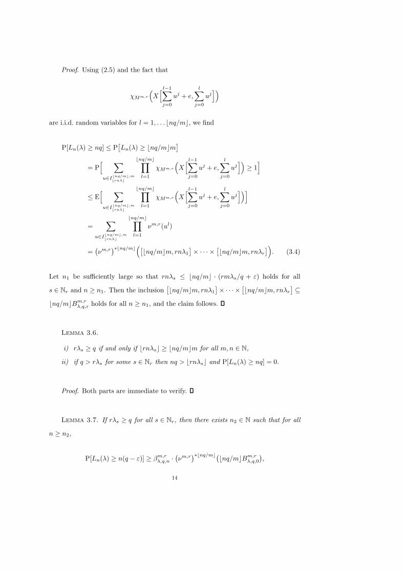
Proof. Using (2.5) and the fact that

*Mm,r

6X/ l'1+

j=0

uj + e,l+

j=0

uj07

are i.i.d. random variables for l = 1, . . . *nq/m+, we find

P[Ln(!) # nq] $ P(Ln(!) # *nq/m+m

)

= P/ +

u%I!nq/m",m!rn""

!nq/m"1

l=1

*Mm,r

6X/l'1+

j=0

uj + e,l+

j=0

uj07# 10

$ E/ +

u%I!nq/m",m!rn""

!nq/m"1

l=1

*Mm,r

6X/l'1+

j=0

uj + e,l+

j=0

uj070

=+

u%I!nq/m",m!rn""

!nq/m"1

l=1

#m,r(ul)

="#m,r#&!nq/m"

6(*nq/m+m, rn!1

)( · · ·(

(*nq/m+m, rn!r

)7. (3.4)

Let n1 be su"ciently large so that rn!s $ *nq/m+ · (rm!s/q + &) holds for all

s ! Nr and n # n1. Then the inclusion(*nq/m+m, rn!1

)( · · ·(

(*nq/m+m, rn!r

)4

*nq/m+Bm,r!,q,# holds for all n # n1, and the claim follows.

Lemma 3.6.

i) r!s # q if and only if *rn!s+ # *nq/m+m for all m, n ! N,

ii) if q > r!s for some s ! Nr then nq > *rn!s+ and P[Ln(!) # nq] = 0.

Proof. Both parts are immediate to verify.

Lemma 3.7. If r!s # q for all s ! Nr, then there exists n2 ! N such that for all

n # n2,

P[Ln(!) # n(q % &)] # 0m,r!,q,n ·"#m,r#&!nq/m""*nq/m+Bm,r

!,q,0

#,

14

where

"0m,r!,q,n

#'1 =r1

s=1

?*rn!s+ % *nq/m+(m% 1)

*nq/m+

@.

Proof. It follows from Lemma 3.6 i) and equation (2.6) that I!nq/m",m!rn!" and

[*nq/m+, rn!1] ( · · · ( [*nq/m+, rn!r] are nonempty sets. For n # n1 := m/& we

have *nq/m+m # n(q % &) and hence,

P(Ln(!) # n(q % &)

)# P(Ln(!) # *nq/m+m

)

(2.5)= P/ +

u%I!nq/m",m!rn""

!nq/m"1

l=1

*Mm,r

6X( l'1+

j=0

uj + e,l+

j=0

uj)7# 10

#"#I!nq/m",m

!rn!"#'1 E/ +

u%I!nq/m",m!rn""

!nq/m"1

l=1

*Mm,r

6X( l'1+

j=0

uj + e,l+

j=0

uj)70

(3.4),(2.6)= 0m,r

!,q,n ·"#m,r#!nq/m"

6(*nq/m+, rn!1

)( · · ·(

(*nq/m+, rn!r

)7

# 0m,r!,q,n ·"#m,r#!nq/m""*nq/m+Bm,r

!,q,0

#.

Lemma 3.8. If r!s # q for all s ! Nr, then

limm#$

limn#$

"0m,r!,q,n

#'1/!nq/m" = 0.

Proof. The proof of Stirling’s formula establishes Robbins’ inequality [14]: for all

n # 1,

82' nn+ 1

2 e'n+ 112n+1 $ n! $

82' nn+ 1

2 e'n+ 112n .

Using this inequality and the shorthand notation k = *nq/m+ and ns = *rn!s+ %

15

*nq/m+(m% 1), we find

r1

s=1

(2') 12k n

'nsk + 1

2ks e'

nsk + 1

(12ns+1)k

(2') 12k k'1+ 1

2k e'1+ 112k2 (2') 1

2k (ns % k)'nsk +1+ 1

2k e'nsk +1+ 1

12(ns#k)k

$"0m,r!,q,n

#' 1k

$r1

s=1

(2') 12k n

'nsk + 1

2ks e'

nsk + 1

12nsk

(2') 12k k'1+ 1

2k e'1+ 1(12k+1)k (2') 1

2k (ns % k)'nsk +1+ 1

2k e'nsk +1+ 1

(12(ns#k)+1)k.

Since ns/k " r!sm/q % (m% 1) when n "-, both sides of the inequality converge

to

r1

s=1

61% q

r!sm'q(m'1)

7 r"smq '(m'1)

r!smq %m

,

and for m"- this tends to<r

s=1(e · limm#$(r!s/q % q)m)'1 = 0.

The stage is now set for a proof of Proposition 3.4:

Proof. i) Using Lemma 3.5, we find

c(!, q) = lim supn#$

P(Ln(!) # nq

)1/n $ lim supn#$

""#m,r#&!nq/m""*nq/m+Bm,r

!,q,#

##1/n

=6lim sup

n#$

""#m,r#&!nq/m""*nq/m+Bm,r

!,q,#

##1/!nq/m"7limn$%

!nq/m"n

< 1q/n.

ii) If q > r!s for some s ! Nr then Lemma 3.6 implies Bm,r!,q,0 = 7, and the claim

holds trivially. On the other hand, if q $ r!s for all s then Lemma 3.8 shows that

there exists m0 such that for all m # m0, limn#$(0m,r!,q,n)'1/!nq/m" < 1, and then

lim supk#$

""#m,r#&k"

kBm,r!,q,0

##1/k

= lim supn#$

"0m,r!,q,0 ·"#m,r#&!nq/m""*nq/m+Bm,r

!,q,0

## 1n · n

!nq/m" · limn#$

"0m,r!,q,n

#'1/!nq/m"

Lem3.7$6lim sup

n#$P[Ln(!) # n(q % &)] 1

n

7limn$%n

!nq/m"= (c(!, q % &))m/q < 1.

16

3.3. Reduction to a Decision Problem. Propositions 3.1 and 3.4 combined

show the following implications: if there exists & > 0 such that

lim supk#$

""#m,r#&k"

kBm,r!,q,#

##1/k< 1 (3.5)

then "(!) $ q. On the other hand, if "(!) < q then there exists m0 such that for all

m # m0 (3.5) holds with & = 0. Thus, all that is needed to determine whether q is

an upper bound on "(!) or not is to decide whether (3.5) holds. In this section we

will show that this decision problem can be replaced by one that is more amenable to

numerical computations. This reformulation uses large deviations theory and convex

analysis.

For all m ! N we denote the log-Laplace transforms of #m,r and #m,r by

$m,r(x) := log,

Rr

#m,r(y) e)y,x* dy,

$m,r(x) := log,

Rr

#m,r(y) e)y,x* dy.

It follows from Lemma 2.1 that both functions are well-defined and finite on an open

domain D 9 Rr that contains the nonpositive orthant Rr' := {x ! Rr : xi $ 0 ,i !

Nr}. In particular, D contains a neighborhood of the origin. Consider the relation

inf4$m,r(x)% rm

q1!, x2 : x ! Rr

'

5< 0. (3.6)

The main result of this section is the following.

Proposition 3.9. For all q > 0, ! ! !r and m ! N,

i) if (3.6) holds then there exists & > 0 such that (3.5) holds,

ii) if (3.5) holds for & = 0 then (3.6) holds.

The following is an interesting immediate consequence of Proposition 3.9.

17

Corollary 3.10. For all q > 0, ! ! !r, m ! N,

i) (3.5) holds for & = 0 if and only if (3.5) holds for some & > 0,

ii) (3.5) with & = 0 is equivalent to (3.6).

We prepare the proof of Proposition 3.9 through a string of preliminaries. Func-

tions that appear throughout this section are proper functions in the sense commonly

used in convex analysis: we allow such functions to take values in R & {+-}. By

default we set f(x) = +- for all x outside the domain dom(f) := {x : f(x) < +-}

of f . A proper function f : Rr " R & {+-} is convex if its epigraph epi(f) :=

{(x, t) ! Rr+1 : t # f(x)} is a convex set. This is equivalent to dom(f) and f |dom(f)

being convex.

Lemma 3.11. $m,r and $m,r are convex on Rr.

Proof. Let us first argue that D is convex. Let x = ,1x1 + ,2x2 be a convex

combination of two elements of D. It su"ces to show that*

Rr #m,r(y) e)y,x* dy is

finite, but this follows immediately from the convexity of x '" exp1y, x2 and the

assumption that x1, x2 ! D. Next, to show that $m,r is convex on D it su"ces to

show that"12/1xj1xk$m,r(x)

#is positive definite for all x ! D. Let u ! Rr, and let

us write 2(x) =*

Rr #m,r(y) e)y,x* dy. Then

D2u,u $

m,r(x) =1

2(x)

,

Rr

#m,r(y) e)y,x*1y, u22dy % 122(x)

6,

Rr

#m,r e)y,x*1y, u2dy72

.

Setting ,(y) = e)y,x*/2 and 3(y) = e)y,x*/21y, u2, we find

D2u,u $

m,r(x) =1

22(x)

6,

Rr

#m,r(y),2(y)dy ·,

Rr

#m,r(y)32(y)dy

%6,

Rr

#m,r(y),(y)3(y)dy727

> 0,

where the last inequality follows from the Cauchy-Schwartz inequality and the fact

that , and 3 are not proportional to one another. The convexity of $m,r follows

immediately from that of $m,r.

18

Lemma 3.12 (Large Deviation Theorem in Rr). Let Sk = Z1 + · · · + Zk be a

sum of k i.i.d. random vectors Zj with values in Rr and law L (Z). Let $Z(x) =

log E(exp1Z, x2

)be the log-Laplace transform of L (Z). If $Z is finite in a neighbor-

hood of the origin and B is a convex subset of Rr, then

limk#$

1k

P[Sk/k ! B] = % infy%B

$&Z(y),

where $&Z(y) = supx%Rr

%1y, x2 % $Z(x)

&is the Legendre transform of $Z .

For a proof of Lemma 3.12, see e.g. [10].

Lemma 3.13 (Fenchel Duality Theorem). For convex proper functions f : Rr "

R & {+-}, g : Rn " R & {+-} and a linear map A : Rr " Rn, if the origin lies in

the interior of dom(g)%A(dom(f)), then

infx%Rr

%f(x) + g(Ax)

&= sup

y%Rn

%%f&(A&y)% g&(%y)

&,

where f& is the Legendre transform of f and A& the adjoint of A.

For a proof of Lemma 3.13, see e.g. Theorem 3.3.5 [5].

We are ready to give a proof of Proposition 3.9:

Proof. i) Let Z1, . . . , Zk be i.i.d. random vectors with distribution L (Zj) = #m,r

on Rr and Sk = Z1 + · · · + Zk. Then

(#m,r)&k"kBm,r

!,q,#

#= #m,r(Rr)k · P

(Sk ! kBm,r

!,q,#

). (3.7)

For x ! Rr let Hm,r,x!,q,# := {z ! Rr : 1z % rm!/q % &e, x2 $ 0}. Then Bm,r

!,q,# 9 Hm,r,x!,q,#

19

for all x ! Rr+ := %Rr

'. Let W #,xj := 1Zj % rm!/q % &e, x2. Then for all x ! Rr

',

P(Sk ! kBm,r

!,q,#

)$ P/Sk/k ! Hm,r,'x

!,q,#

0= P

A

Bk+

j=1

W #,'xj $ 0

C

D

$ E/e'

Pkj=1 W #,#x

j

0=6E/e'W #,#x

1

07k=6,

Rr

#m,r(y) e)y'rm!/q'#e,x* dy7k

.

Together with (3.7) this shows that for all k ! N, x ! Rr',

6"#m,r#&k"

kBm,r!,q,#

#71/k$,

Rr

#m,r(y) e)y'rm!/q'#e,x* dy

= exp?%&1e, x2+ $m,r(x)% rm

q1!, x2@

.

The claim of part i) now follows immediately.

ii) Theorem 3.12 shows that

limk#$

1k

log P/Sk ! kBm,r

!,q,0

0= sup

y%Bm,r",q,0

%$m,r&(y).

Therefore, (3.7) implies

limk#$

1k

log6"#m,r#&k"

kBm,r!,q,0

#7= #m,r(Rr) + lim

k#$

1k

log P/Sk ! kBm,r

!,q,0

0

= #m,r(Rr) + supy%Bm,r

",q,0

%$m,r&(y)

= supy%Rr

{%$m,r&(y)% g&(%y)} , (3.8)

where

g&(y) =

899:

99;

0 if y ! %Bm,r!,q,0,

+- otherwise.

It is easy to check that g& is a convex proper function with Legendre transform

g(x) = g&&(x) = supy%Rr

{1x, y2 % g&(y)} = supy%'Bm,r

",q,0

1x, y2.

20

Since the origin lies in the interior of dom(g)%D, Theorem 3.13 establishes that

supy%Rr

{%$m,r&(y)% g&(%y)} = infx%Rr

-$m,r(x) + sup

y%'Bm,r",q,0

1x, y2.

. (3.9)

For x ! Rr let Jx := {j ! Nr : xj > 0}. Then – using LP duality or by inspection –

it is easy to check that

supy%'Bm,r

",q,0

1x, y2 = %m+

j%Jx

xj %rm

q

+

j%Jcx

!jxj .

We claim that if there exists j0 ! Jx then %ej0 is a descent direction for the function

2(x) := $m,r(x) + supy%'Bm,r

",q,0

1x, y2.

In fact,

d

dt|t=02(x% tej0) =

*Rr #m,r(y) · e)y,x* ·(%yj0)dy*

Rr #m,r(y) e)y,x* dy+ m < 0,

where the last inequality follows from the fact that #m,r(y) > 0 implies yj0 # m.

Therefore,

infx%Rr

-$m,r(x) + sup

y%'Bm,r",q,0

1y, x2.

= infx%Rr

#

E$m,r(x) % rm

q1!, x2F

. (3.10)

The claim of part ii) now follows from (3.8), (3.9) and (3.10).

3.4. A Consistent Sequence of Upper Bounds. By now we have built up

all the necessary tools to present and prove the main result of Section 3 which shows

that

qm(!) = inf%q > 0 : inf

%$m,r(x)% (rm/q)1!, x2 : x ! Rr

'&

< 0&

(3.11)21

defines a consistent sequence"qm(!)#

m%N of upper bounds on "(!).

Theorem 3.14. For all ! ! !r,

i) "(!) $ qm(!) for all m ! N,

ii) limm#$ qm(!) = "(!).

Proof. i) It su"ces to show that if q > 0 is such that (3.6) holds then "(!) $ q.

If (3.6) holds, then by Proposition 3.9 i) there exists & > 0 such that (3.5) holds, and

by Proposition 3.4 i) this implies c(!, q) < 1. Finally, Proposition 3.1 establishes that

"(!) $ q.

ii) It su"ces to prove that for all q > "(!) there exists m0 such that q # qm

for all m # m0. Let & = (q % "(!))/2 > 0. Then q % & > "(!) and Proposition 3.1

ii) implies c(!, q % &) < 1. By Proposition 3.4 ii) there exists m0 such that for all

m # m0,

lim supk#$

""#m,r#&k"

kBm,r!,q,0

##1/k< 1.

Finally, Proposition 3.9 ii) shows that (3.6) holds, implying that q # qm for all

m # m0, as claimed.

In [11] it was established that in the special case r = 2 and ! = (0.5, 0.5) the

approximation error qm(!) % "(!) converges to zero at the rate O(m' 1##2 ), for & > 0

arbitrary. We believe that the same order holds true in the general case, but we will

not pursue this issue further here because this bound is too conservative in practical

computations, and furthermore it is a theoretical result that only holds for large m

which are beyond the scope of our numerical experiments.

4. Monte Carlo Simulation and Numerical Results. In Section 3 we saw

how to construct a consistent sequence (qm(!))m%N of upper bound functions on the

mean curve "(!). So far this is only a theoretical tool, as the measure #m,r is not

known. To turn this into a practical method for the computation of upper bounds,22

#m,r has to be replaced by an approximation G#m,r obtained by Montecarlo simulation

as follows: for $ = 1, . . . , $0 let X" ="(X1

",n)n%N, . . . , (Xr",n)n%N

#be independent copies

of r-tuples of random sequences with the required distribution. For all multi-indices

i ! Nr set

G#m,r(i) =1$0

· |{$ : X"[e, i] !Mm,r}| .

Note that this is possible to compute because almost surely only finitely many terms

of each X" have to be simulated to find all i ! Nr for which X"[e, i] !Mm,r. Further-

more, since #m,r(i) decreases exponentially in |i| (see proof of Lemma 2.1), G#m,r(i) > 0

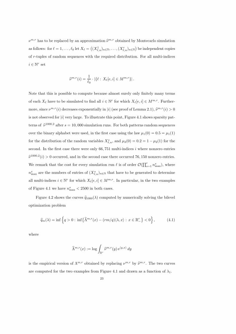
is not observed for |i| very large. To illustrate this point, Figure 4.1 shows sparsity pat-

terns of G#1000,2 after s = 10, 000 simulation runs. For both patterns random sequences

over the binary alphabet were used, in the first case using the law µ1(0) = 0.5 = µ1(1)

for the distribution of the random variables Xs",n, and µ2(0) = 0.2 = 1%µ2(1) for the

second. In the first case there were only 66, 751 multi-indices i where nonzero entries

G#1000,2(i) > 0 occurred, and in the second case there occurred 76, 150 nonzero entries.

We remark that the cost for every simulation run $ is of order O(<r

s=1 nsmax), where

nsmax are the numbers of entries of (Xs

",n)n%N that have to be generated to determine

all multi-indices i ! Nr for which X"[e, i] !Mm,r. In particular, in the two examples

of Figure 4.1 we have nsmax < 2500 in both cases.

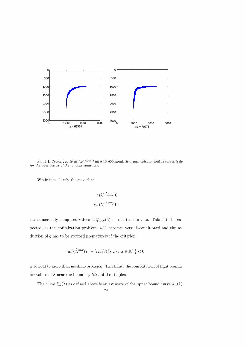
Figure 4.2 shows the curves Gq1000(!) computed by numerically solving the bilevel

optimization problem

Gqm(!) = inf4q > 0 : inf

%G$m,r(x)% (rm/q)1!, x2 : x ! Rr'&

< 05

, (4.1)

where

G$m,r(x) := log,

Rr

G#m,r(y) e)y,x* dy

is the empirical version of $m,r obtained by replacing #m,r by G#m,r. The two curves

are computed for the two examples from Figure 4.1 and drawn as a function of !1.

23

0 1000 2000 3000

0

500

1000

1500

2000

2500

3000

nz = 623640 1000 2000 3000

0

500

1000

1500

2000

2500

3000

nz = 70775

Fig. 4.1. Sparsity patterns for b!1000,2 after 10, 000 simulation runs, using µ1 and µ2 respectivelyfor the distribution of the random sequences.

While it is clearly the case that

"(!) !1#0%" 0,

qm(!) !1#0%" 0,

the numerically computed values of Gq1000(!) do not tend to zero. This is to be ex-

pected, as the optimization problem (4.1) becomes very ill-conditioned and the re-

duction of q has to be stopped prematurely if the criterion

inf%G$m,r(x)% (rm/q)1!, x2 : x ! Rr

'&

< 0

is to hold to more than machine precision. This limits the computation of tight bounds

for values of ! near the boundary 1!r of the simplex.

The curve Gqm(!) as defined above is an estimate of the upper bound curve qm(!)24

0.4 0.45 0.5 0.55 0.60.76

0.77

0.78

0.79

0.8

0.81

0.82

0.83

0.4 0.45 0.5 0.55 0.60.78

0.8

0.82

0.84

0.86

0.88

0.9

Fig. 4.2. Numerically computed upper bounds bqm(") for the examples of Figure 4.1. The ploton the left corresponds to µ1, the one on the right to µ2. The accuracy of approximation getsgradually worse for " near the boundary.

derived in Section 3. Note however that we did not yet determine a confidence level

for the event that Gqm(!) is an upper bound on "(!). To determine such a confidence

level we need to simulate G#m,r several times independently. In our experiments we

computed 20 independent copies G#1, . . . , G#20 of G#1000,2 with $0 = 500 simulation runs

each. Each of the measures G#k defines an empirical analogue

G$k(x) := log,

Rr

G#k(y) e)y,x* dy

of $m,r. For fixed values of q and ! this defines i.i.d. random variables

Ik(q,!) := inf4G$k(x)% (rm/q)1!, x2 : x ! Rr

'

5

that are close to normally distributed but with a slightly tighter concentration of mass

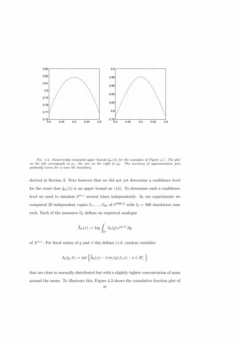
around the mean. To illustrate this, Figure 4.3 shows the cumulative fraction plot of25

!0.6 !0.4 !0.2 0 0.20

0.2

0.4

0.6

0.8

1

!0.8 !0.6 !0.4 !0.2 0 0.20

0.2

0.4

0.6

0.8

1

!2 !1.5 !1 !0.5 0 0.50

0.2

0.4

0.6

0.8

1

!2 !1.5 !1 !0.5 0 0.50

0.2

0.4

0.6

0.8

1

Fig. 4.3. Cumulative fraction plots of Ik(q, ") versus the cumulative distribution of normaldistributions with the estimated mean and variance. The plots of column 1 are based on µ1 andthose of column 2 on µ2. In row 1 the value "1 = 0.47 was used, whereas "1 = 0.5 was used in thesecond row. In all four plots the computed value of bq95%

m (") was used for q.

Ik(q,!) (k = 1, . . . , 20) for several values of q and !, both for µ1 and µ2 (as introduced

above), along with the cumulative distribution plot of N"mean(I1, . . . , I20), var(I1, . . . , I20)

#,

where mean and var are the empirical mean and variance respectively.

Let J(q,!) denote a random variable with law

L (J(q,!)) = N"mean(I1, . . . , I20), var(I1, . . . , I20)

#.

An approximate 95%-confidence-level upper bound on "(!) can be computed as

follows,

Gq95%m (!) = inf {q > 0 : |{k : Ik < 0}| # 19} .

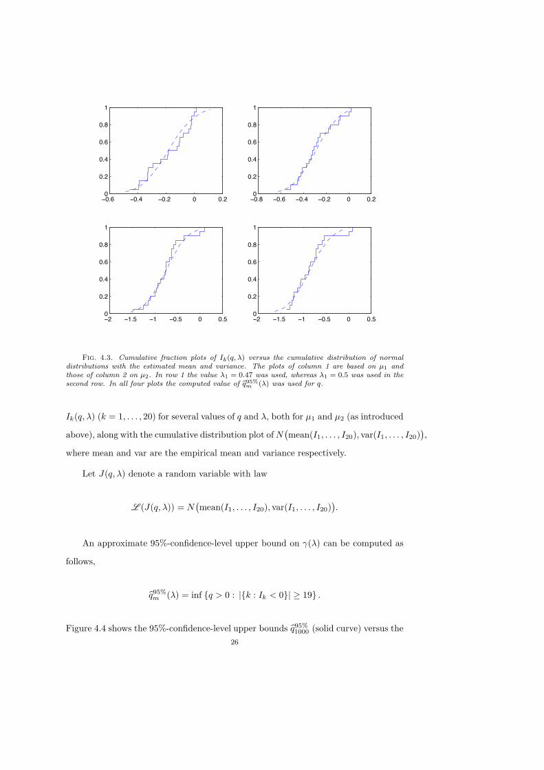
Figure 4.4 shows the 95%-confidence-level upper bounds Gq95%1000 (solid curve) versus the

26

0.49 0.495 0.5 0.505 0.510.8175

0.818

0.8185

0.819

0.49 0.495 0.5 0.505 0.510.8795

0.88

0.8805

0.881

0.8815

0.882

0.8825

0.883

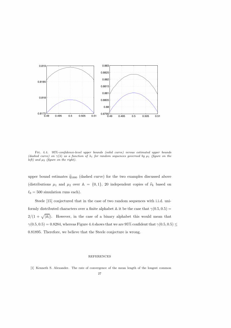
Fig. 4.4. 95%-confidence-level upper bounds (solid curve) versus estimated upper bounds(dashed curve) on #(") as a function of "1 for random sequences governed by µ1 (figure on theleft) and µ2 (figure on the right).

upper bound estimates Gq1000 (dashed curve) for the two examples discussed above

(distributions µ1 and µ2 over A = {0, 1}, 20 independent copies of G#k based on

$0 = 500 simulation runs each).

Steele [15] conjectured that in the case of two random sequences with i.i.d. uni-

formly distributed characters over a finite alphabet A it be the case that "(0.5, 0.5) =

2/(1 +H|A|). However, in the case of a binary alphabet this would mean that

"(0.5, 0.5) = 0.8284, whereas Figure 4.4 shows that we are 95% confident that "(0.5, 0.5) $

0.81895. Therefore, we believe that the Steele conjecture is wrong.

REFERENCES

[1] Kenneth S. Alexander. The rate of convergence of the mean length of the longest common

27

subsequence. Ann. Appl. Probab., 4(4):1074–1082, 1994.

[2] Richard Arratia and Michael S. Waterman. A phase transition for the score in matching random

sequences allowing deletions. Ann. Appl. Probab., 4(1):200–225, 1994.

[3] K. Azuma. Weighted sums of certain dependent random variables. Tohuku Math. J., 19:357–

367, 1967.

[4] R.A. Baeza-Yates, R. Gavalda, G. Navarro, and R. Scheihing. Bounding the expected length

of longest common subsequences and forests. Theory Comput. Syst., 32(4):435–452, 1999.

[5] J.M. Borwein and A.S. Lewis. Convex Analysis and Nonlinear Optimization. Springer, New

York, 2000.

[6] Vaclav Chvatal and David Sanko!. Longest common subsequences of two random sequences.

J. Appl. Probability, 12:306–315, 1975.

[7] Vlado Dancık and Mike Paterson. Upper bounds for the expected length of a longest common

subsequence of two binary sequences. Random Structures Algorithms, 6(4):449–458, 1995.

[8] Quentin Decouvelaere. Upper Bounds for the LCS Problem. MSc Thesis, Oxford University

Computing Laboratory, 2003.

[9] Joseph G. Deken. Some limit results for longest common subsequences. Discrete Math.,

26(1):17–31, 1979.

[10] Frank den Hollander. Large Deviations, volume 14 of Fields Institute Monographs. American

Mathematical Society, Providence, RI, 2000.

[11] Raphael Hauser, Servet Martinez, and Heinrich Matzinger. Large deviation based upper bounds

for the lcs problem. Technical Report NA03/13 Oxford University Computing Laboratory,

2003.

[12] W. Hoe!ding. Probability inequalities for sums of bounded random variables. J. Amer. Statis.

Assoc., 58:13–30, 1963.

[13] Mike Paterson and Vlado Dancık. Longest common subsequences. In Mathematical foundations

of computer science 1994 (Kosice, 1994), volume 841 of Lecture Notes in Comput. Sci.,

pages 127–142. Springer, Berlin, 1994.

[14] H. Robbins. A remark on stirling’s formula. Amer. Math. Monthly, 62:26–29, 1955.

[15] Michael J. Steele. An efron-stein inequality for nonsymmetric statistics. Ann. Statist., 14:753–

758, 1986.

[16] Robert A. Wagner and Michael J. Fischer. The sring-to-string correction problem. J. Ass.

Comp. Mach., 21:168–173, 1974.

[17] M. Waterman. Introduction to Computational Biology. Chapman & Hall, 1995.

28