
Improving Techniques and Practices on the Geotechnical Centrifuge. Including literature review

f t .F ESL-TR-87-23
A LITERATURE REVIEW OFGEOTECHNICAL CENTRIFUGEMODELING WITH PARTICULAREMPHASIS ON ROCK MECHANICS
P.J. JOSEPH, H.H. EINSTEIN, R.V. WHITMAN
MASSACHUSETTS INSTITUTE OF TECHNOLOGYDEPARTMENT OF CIVIL ENGINEERINGCAMBRIDGE, MASSACHUSETTS 02139JUNE 1988 DTICFINAL REPORT ELECTE -
APRIL 1986 - DECEMBER 1986 S OCT 3 01989 L_ DC
APPROVED FOR PUBLIC RELEASE: DISTRIBUTION UNLIMITED
ENGINEERING & SERVICES LABORATORYAIR FORCE ENGINEERING & SERVICES CENTERTYNDALL AIR FORCE BASE, FLORIDA 32403
89 10 27 1 .0

NOTICE
PLEASE DO NOT REQUEST COPIES OF THIS REPORT FROM
HQ AFESC/RD (ENGINEERING AND SERVICES LABORATORY).
ADDITIONAL COPIES MAY BE PURCHASED FROM:
NATIONAL TECHNICAL INFORMATION SERVICE
5285 PORT ROYAL ROAD
SPRINGFIELD, VIRGINIA 22161
FEDERAL GOVERNMENT AGENCIES AND THEIR CONTRACTORS
REGISTERED WITH DEFENSE TECHNICAL INFORMATION CENTER
SHOULD DIRECT REQUESTS FOR COPIES OF THIS REPORT TO:
DEFENSE TECHNICAL INFORMATION CENTER
CAMERON STATION
ALEXANDRIA, VIRGINIA 22314
Im

UNCLASSIFIEDSECURITY CLASSIFICATION OF THIS PAGE
Form ApprovedREPORT DOCUMENTATION PAGE OMB No. 070-0188
I. REPORT SECURITY CLASSIFICATION lb. RESTRICTIVE MARKINGSUNCLASS I FIED2a. SECURITY CLASSIFICATION AUTHORITY 3. DISTRIBUTION/AVAILABILITY OF REPORT
2b. DECLASSIFICATION /DOWNGRADING SCHEDULE Approved for public releaseDistribution unlimited
4. PERFORMING ORGANIZATION REPORT NUMBER(S) S. MONITORING ORGANIZATION REPORT NUMBER(S)
ESL-TR-87-236a. NAME OF PERFORMING ORGANIZATION 6b. OFFICE SYMBOL 7a. NAME OF MONITORING ORGANIZATIONMassachusetts Institute of (if applicable)Technology Air Force Engineering and Services Center6c. ADDRESS (City, State, and ZIP Code) 7b. ADDRESS (City. State, and ZIP Code)
Department of Civil Engineering HQ AFESC/RDCSCambridge, Massachusetts 02139 Tyndall Air Force Base, Florida 32403-6001
1a. NAME OF FUNDING/SPONSORING 8b. OFFICE SYMBOL 9. PROCUREMENT INSTRUMENT IDENTIFICATION NUMBERORGANIZATION (if applicable)
I Contract # DACA88-86-D-00138c. ADDRESS (City, State, and ZIP Code) 10. SOURCE OF FUNDING NUMBERS
PROGRAM PROJECT TASK WORK UNITELEMENT NO. NO. NO ACCESSION NO.
6.2 2673 0074 N/A11. TITLE (include Security Classification)A Literature Review of Geotechnical Centrifuge Modeling with Particular Emphasis onRock Mechanics
12. PERSONAL AUTHOR(S)P. G. Joseph, H. H. Einstein, R. V. Whitman13a. TYPE OF REPORT 13b. TIME COVERED 114. DATE OF REPORT (YearMonth, Day) 11S. PAGE COUNTFinal IFROM Arr 86 TOQt j June 1988 I120
16. SUPPLEMENTARY NOTATION
Availability of this report is specified on reverse of front cover.
17. COSATI CODES 18. SUBJECT TERMS (Condnue on reverse ff neceuary and identify by block number)
FIELD GROUP SUBGROUP otechnical Centrifuge Modeling Rock MechanicsSmall-Scale Modeling Literature Review -
I9. ABSTRACT (Continue on reverse if necessary and identify by block number)
'Small-scale modeling of structural and geotechnical problems has a long history. Centrifugemodeling plays an increasingly important role in this context. This report summarizesgeotechnical centrifuge work which has been done up to now with particular emphasis on rockmechanics. The reader will first be familiarized with the basic principles of small-scaleand centrifuge modeling. In particular, the scaling relations based on first principles andon dimensional analysis are discussed in detail. Problematic aspects are mentioned andpossible solutions are described. The second chapter is the sunnary of geotechnicalcentrifuge work. While the soils work is mentioned, it is in the form of an overview; incontrast rock mechanics and associated centrifuge research are more completely described.The report then provides the reader with a good background in the principles and applicationof geotechnical centrifuge modeling, while simultaneously creating the basis for theparallel report in which scaling relations for rock centrifuge modeling are established.
20. DISTRIBUTION/AVAILABII 1-V MC aBSTRAT, 21. ABSTRACT SECURITY CLASSIFICATION
IMUNCLASSIFIED/UNLMIfED 0 SAME AS RPT. 0 OTIC USERS UNCLASSIFIED14t E .?F 7PE 1 DUAL' LE9N gde Area Code) ] SYMBOLZt, UJSAF ORISL:N O 83-¢de (FESC/RDCS
DD Form 1473. JUN 86 Previous editions are obsolete. SECURITY CLASSIFICATION OF THIS PAGE
I
(The reverse of this page is blank)
PREFACE
This report was submitted as a dissertation to Massachusetts Institute ofTechnolog, funded under Job Order Number 26730074 by the Air Force Engineeringand Services Center, Engineering and Services Laboratory, Tyndall AFB, Florida32403-6001.
This dissertation is being published in its original format by thislaboratory because of its interest to the worldwide scientific and engineeringcommunity. This dissertation covers work performed between April 1986 andDecember 1986. AFESC/RD project officers were Paul L. Rosengren, Jr., and lLtSteven T. Kuennen.
This report has been reviewed by the Public Affairs Officer (PA) and isreleasable to the National Technical Information Service (NTIS). At NTIS, itwill be available to the general public, including foreign nationals.
TA s technical report has been reviewed and is approved for publication.
S EN T. ENNEN, 2Lt, USAF RIB J. MAJ, C USAFProject Officer Chief, Engineering Re arch Division
WILLIAM S. STRICKLAND, GM-14 JAMES R. VAN ORMANChief, Facility Systems and Deputy Director of Engineering
Analysis Branch and Services Laboratory' ISPECTED
4
o is(The reverse of this page is blank)

Table of Contents
Page Number
Chapter 1 Model Testing Using the Centrifuge 1
1.1 Introduction 1
1.2 The Theory of Centrifuge Modeling 4
1.3 Advantages of Centrifuge Testing 22
1.4 Use of Scaled Model Tests 23
1.5 Pelationship between Prototype and Model 24
1.6 Summary 55
Chapter 2 Geotechnical Applications of the Centrifuge 57
2.1 Introduction 57
2.2 Soil Mechanics 57
2.3 Rock Mechanics 65
2.4 Ice Mechanics 96
2.5 Tectonics 100
2.6 Conclusion 103
References 108
(The reverse of this page is blank.)
v

1
Chapter 1
Model Testing Usinq the Centrifuge
1.1 Introduction
Small scale models are a relatively inexpensive and convenient way of
studying prototype behaviour. Consequently, they have been used extensively
in various fields of engineering. In certain prototypes, however, stresses
due to self weight play a major role, and so, should be reproduced to scale in
the model. This can be done by placing the model in a centrifuge.
Probably the earliest mention of a centrifuge to simulate self weight
effects was by Phillips (1869) who suggested that it be used to simulate self
weight stresses in structural beams. As this was a relatively minor problem,
the use of a centrifuge for modelling was not further pursued until Bucky
(1931) used the centrifuge to study mining problems. Independently of Bucky,
two Russian scientists, Pokrovsky (1933) and Davidenkov (1933) came up with
the same idea. In the following decades, only a few centrifuge research
projects were pursued in the U.S., namely, those by Panek (1949) and Clark
(late fifties and early sixties), in Rock Mechanics. In Russia, however, the
centrifuge seems to have seen frequent use, although oriented toward specific
design problems rather than providing basic input.
Early centrifuge work outside the U.S. and Russia was done by Ramberg
(1963) in Sweden, to study gravity tectonics, and by Hoek (1965) in South
Africa, to study the effect of gravitational force fields in mine models.
In England, Professor Schofield and his colleagues at the University of
Cambridge built a prototype machine in 1966. Professor Schofield continued
his work at the University of Manchester Institute of Science and Technology
where he built a 1.5 m centrifuge in 1969. In the early 1970's, Professor
Peter Rowe built a much larger capacity machine also at the University of
2
Manchester, in the Simon Engineering laboratory. In the meantime, Professor
K. H. Roscoe at Cambridge University had been given f40,000 towards the
construction of a centrifuge with a 10 m rotor arm. In 1974, Professor
Schofield rejoined Cambridge University and took charge of the group.
Thereafter, centrifuge testing of problems involving soil started in earnest,
with various professors from other countries visiting Cambridge to study the
centrifuge technique. During this period, Japan, Denmark, Sweden, Netherlands
and France developed centrifuge mod.,lling facilities.
In the midseventies, in the U.S.A., there was a renewed interest in
centrifuge modeling of geotechnical problems. Professor R.F. Scott was active
in centrifuge modeling in 1975. The University of California at Davis
obtained a I meter radius centrifuge in 1976. Dr. R.M. Schmidt of Boeing
started craterinq experiments on a 1-meter centrifuge in 1976. In 1979, the
National Science Foundation funded the modification of a large centrifuge
located at NASA Ames Research Centre, Mountain View, California, for use in
research in geotechnical engineering. As of this date, the centrifuge is not
yet ready. When complete, it will have a nominal radius of 30 feet and carry
6,000 lbs. of soil at 300 g's and with subsequent modification, 40,000 lbs. at
100 g's, thus making it the largest capacity centrifuge in the U.S.A. As of
now, several universities in the U.S. have developed or are in the process of
developing centrifuge facilities for geotechnical research. The University of
California at Davis has been proposed as a center for Geotechnical Centrifuge
modeling. The goals of this center will be to foster centrifuge modeling in
the U.S.A. and to serve as a resource for experimenters in this field.
3
This report will cover the principles, advantages, and problems of
centrifuge testing. It will discuss the use of scaled model tests, the
various relationships between the model and prototype, and how to obtain them.
It will examine the various uses that the centrifuge has been put to, for
modelling soil, rock and ice behaviour, and for studying gravity tectonics.

4
1.2 The Theory of Centrifuge Modelling
This section will examine the basic theory on which centrifuge modelling
is based. The underlying principle is that stresses at geometrically similar
points in prototype and model should be the same. Bucky (1931) suggested a
method for doing this: "To produce at corresponding points in a small
scale model, the same unit stresses that exist in a full scale structure, the
weight of the material of the model must be increased in the same ratio that
the scale of the model is decreased with respect to the full scale structure.
The effect of an increase in weight may be obtained by the use of centrifugal
force, the model being placed in a suitable revolving apparatus." If the
model and prototype are made of materials with identical mechanical
properties, then the strains in the model and prototype will also be
identical. In other words, if a-L scale model of a prototype is spun at Ng on
the centrifuge, then the model's behaviour is thought to be similar to the
prototype's behaviour. For this to hold true, three assumptions must be
satisfied. These are: 1) that the model is a correctly scaled version of the
1prototype; 2) that thel scaled model when subject to an ideal Na gravity
field (such as that acting on the surface on an Nq planet), behaves like the
prototype at Ig; and 3) that the centrifuge produces this ideal gravitational
field. These three assumptions will be examined in detail in the following
sections. Emphasis will be placed on commenting on the effects which result
from not fully satisfying the assumptions.
1.2.1 Assumption One
This assumption is that the model is an exactly scaled version of the
prototype, which requires that the scaling relations between the model and
prototype be satisfied. Such scaling relationships are obtained from either a

5
dimensional analysis of the relevant variables, or from consideration of the
governing equation. The details of the two scaling approaches will be
discussed later, while a summary is provided here:
If the suffixes 'p' and 'm' stand for prototype and model respectively,
arnd Lp and Lm represent the length of the prototype and the length of the
model respectively, then the relation
L-E-= N (1.1)L
m
is a scaling relation and 'N' is the scale factor. Analogous scaling
relations can be established for other properties i.e.: unit weight,
velocity, acceleration, etc., whose scale factors may be the same as the scale
factor for length, or may be different. In many cases however, exact
similitude between model and prototype is not possible. In such cases,
variables whose effects are known or which influence the behaviour in a
relatively minor way, are allowed to deviate from their scaled values.
Scaling down a prototype, especially with large scale factors, may result
in a loss of prototype detail. In some cases this may not be of importance,
while in others, it may be crucial. For example, i., centrifuge modelling of
gravity tectonics processes, the value of the scale factor 'N' is of the order
of 104 [Ramberg (1965)]. In such a situation, modelling of a rock layer a few
feet thick is not possible for reasons of practicality. However, since the
structures being modelled have dimensions in the order of miles, this
departure from exactness is not likely to influence results. In other cases,
however, this may not be true. For example, thin seams in the prototype may
control the behaviour being studied, and consequently will have to be
correctly scaled and included in the model.

6
Scaling down a prototype may also result in parameters, which do not have
an effect on prototype behaviour, significantly influencing model behaviour.
These effects are known as scale effects since they arise as a result of
scaling done to the prototype. For example, in studies of footing
behavior using the centrifuge, the soil material is usually not scaled in
grain size. In such a case, the model footing may be scaled down to the
extent that the individual size of the grains would begin to affect the
footing behaviour. Scale effects occur to some extent in all models. Their
effects are reduced, by building the model as large as possible. One way to
guard against scale effects is to check what is called the 'Internal
Consistency' of the experiment using the 'Modelling of Models' technique.
This technique consists of modelling the same prototype at different scales,
by choosing the g level for each scale such that the product of each scale
factor and its corresponding g level is always the same. So, if the results
of a 1 scale model of a particular prototype, tested at 100g are the same100
as those of a 1- scale model of the same prototype tested at 20g, then one
can conclude that the scale effects are not significant. Examples of
parameters that could result in scale effects are grain size and surface
roughness.
Apart from loss of prototype detail and scale effects, it may not be
pcssible to model certain prototype characteristics. For example, the crystal
structure of model ice may differ from that of the arctic sea ice being
modelled. In such cases it has been suggested that results from the tests
using model ice be modified analytically to account for the difference in ice
crystal structure (Vinson (1982)].

7
1.2.2 Assumption Two
This assumption is that the L scale model when subject to an ideal Ng
gravity field (such as that acting on the surface of an Ng planet), behaves
like the prototype at 1g. This assumption requires that for a correctly
scaled model (see 1.2.1), the model material at 17g has the same material
properties as the model material £' ig since the scaling is done on the basis
of the material propet'ies at 1g. It also requires that the ohenomena that
occur in the prototype at Ig occur in the model at Ng. Each of these
conditions can be examined in greater detail:
Schofield (1980) states that whatever the model material, its material
properties do not change as the g level changec. Material properties, apart
from the self-weight, are determined by the electron shells of the atoms of
the materials involved. When the g field changes, the effects are felt at the
centre of the mass of the atom, and not at the electron shells. Consequently,
though the unit weight of the material may change, the material properties at
Ng remain unaltered from those at 1g.
While the material -cperties may remain unaltered, phenomena that occur
in a prototype at Ig may not always be reproduced in a correctly scaled model
at Ng. Tan and Scott (1985; examined the case of a soil particle moving in a
cuid and, as will be explained later, showed that behaviour in the Ng field
was not the same as in a Ig field.
1 .2.3 Assumption Three
This assumption is that the centrifuge produces an ideal Ng gravitational
field. An ideal gravitational field is considered to be the gravitational
8
field acting on the surface of an Ng planet. The earth can be considered an
Ng planet, where N=1. Any mass resting on the surface of such a planet is
subject to two forces that give it its weight. One force is the centrifugal
force due to rotation of the planet about its axis while the other is due to
gravity and is given by Newton's law of universal gravity. Thus the force
acting on a body on the surface of a planet like the earth is given as
G1I 2 2
F 2 m w r (1.2)21
r
where
F = Force acting on the mass resting on or in the earth
m, = Mass of the body on or in the earth
m 2 = Mass of the earth
r = The radius of the earth at that point
w = Angular velocity of rotation of the earth
G = The universal gravitational constant.
G mI m2in comparison with the quantity 2 , the quantity m, w2 r is so
r
small that it can be neglected. Also, it can be seen that the gravitational
field on a planet is not a constant, but varies with distance from the center
ot the earth. However, up to depths normally encountered in geotechnical
engineering, this change is so small that it can be neglected. Consequently,
for normal ci t engineering purposes, the acceleration due to gravity is
consider-d -1 -ant, throughout the prototype.
9
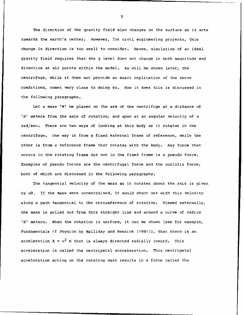
The direction of the gravity field also changes on the surface as it acts
towards the earth's center. dowever, for civil engineering projects, this
change in direction is too small to consider. Hence, simulation of an ideal
gravity field requires that the g level does not change in both magnitude and
direction at all points within the model. As will be shown later, the
centrifuge, while it does not provide an exact replication of the above
conditions, comes very close to doing so. How it does this is discussed in
the following paragraphs.
Let a mass 'M' be placed on the arm of the centrifuge at a distance of
'R' meters from the axis of rotation, and spun at an angular velocity of W
rad/sec. There are two ways of looking at this body as it rotates in the
centrifuge. One way is from a fixed external frame of reference, while the
other is from a reference frame that rotates with the body. Any force that
occurs in the rotating frame but not in the fixed frame is a pseudo force.
Examples of pseudo forces are the centrifugal force and the coriolis force,
both of which are discussed in the following paragraphs.
The tangential velocity of the mass as it rotates about the axis is given
by wR. If the mass were unrestrained, it would shoot out with this velocity
along a path tangential to the circumference of rotation. Viewed externally,
the mass is pulled out from this straight line and around a curve of radius
'R' meters. When the rotation is uniform, it can be shown [see for example,
Fundamentals cf Physics by Halliday and Resnick (1981)], that there is an
acceleration A = ,I2 R that is always directed radially inward. This
acceleration is called the centripetal accceleration. This centripetal
acceleration acting on the rotating mass results in a force called the
10
centripetal force. Since this force acts in a fixed frame, it is a real
force. When the reference frame rotates with the mass on the centrifuge,
there will be a force acting radially outwards that is equal in magnitude to
the centripetal force, but opposite in direction. This is the centrifugal
force, and since it exists only in a moving reference frame, it is a pseudo
force. The various forces are shown in Figure 1.1.
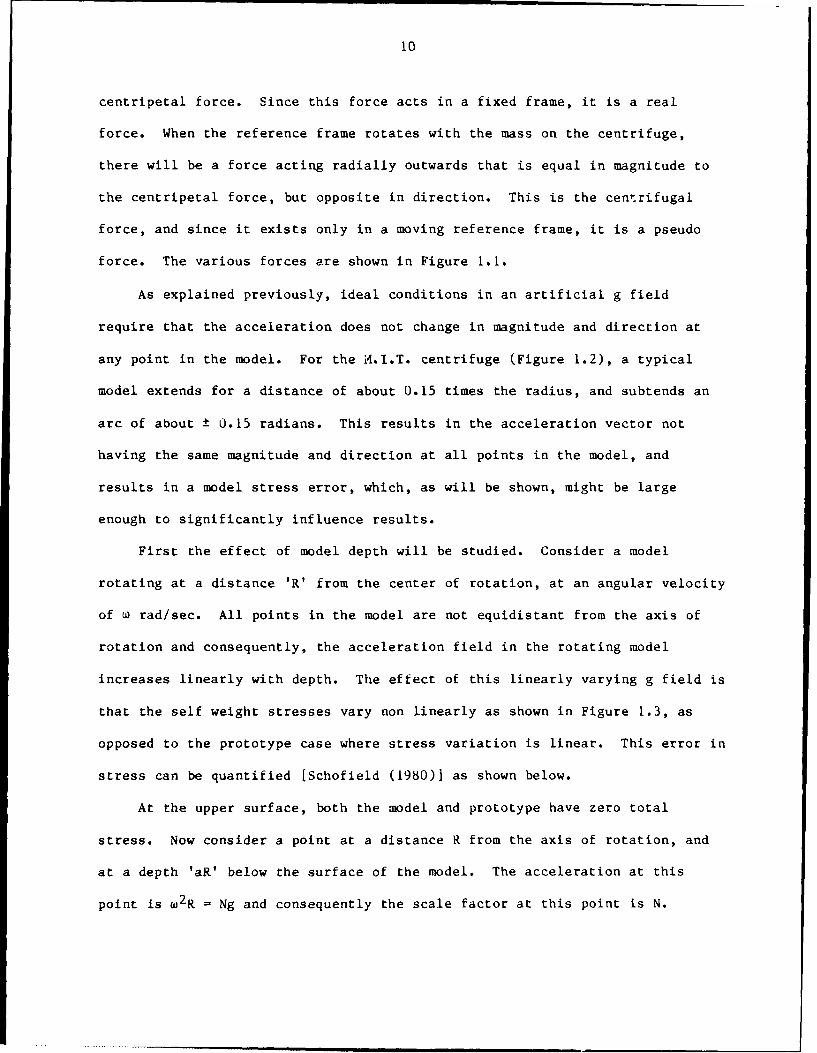
As explained previously, ideal conditions in an artificial g field
require that the acceleration does not change in magnitude and direction at
any point in the model. For the M.I.T. centrifuge (Figure 1.2), a typical
model extends for a distance of about 0.15 times the radius, and subtends an
arc of about ± 0.15 radians. This results in the acceleration vector not
having the same magnitude and direction at all points in the model, and
results in a model stress error, which, as will be shown, might be large
enough to significantly influence results.
First the effect of model depth will be studied. Consider a model
rotating at a distance 'R' from the center of rotation, at an angular velocity
of w rad/sec. All points in the model are not equidistant from the axis of
rotation and consequently, the acceleration field in the rotating model
increases linearly with depth. The effect of this linearly varying g field is
that the self weight stresses vary non linearly as shown in Figure 1.3, as
opposed to the prototype case where stress variation is linear. This error in
stress can be quantified [Schofield (1980)] as shown below.
At the upper surface, both the model and prototype have zero total
stress. Now consider a point at a distance R from the axis of rotation, and
at a depth 'aR' below the surface of the model. The acceleration at this
point is w2R = Ng and consequently the scale factor at this point is N.

11
L
10L~1
C
xCu
.IJ
0
'U
-I
'U
0
>1
0.0CU
0C0
__ 4,o ___ 0Cu
4-0
0U
0
-4
-4
0*

12
Fig.l.2. The M.I.T. Centrifuge
SOIL P1RESSTUmE
R
R/15 UNE STRESS
L DEPITR
R/ 30
T BOTMOVER STRES
Fig. 1.3. Model stress error with depth. From. Schofield (1980)

13
For the prototype, this point would correspond to a point at a depth NaR. The
vertical stress at this point in the prototype would be
av = pg N a R (1.3)
where p is the mass density of the prototype material.
For the model in the centrifuge, however, the vertical stress at this point is
given by an integration to the depth 'aR', since the acceleration field from
R-aR = R (1-a) (the radius to the ground surface) to R is not constant.
Consequently, the stress at this point in the model is given by
rR 2
f pW2 r drR(1-a)
2 r 21 R2 R - aR2
= 0 ,2 [R2 - R2 + 2a R2 - a2 R2 ]
2
= p W2 a R2 (2 - a) (1.4)2
Equating 1.3 and 1.4
pg N a R =p W a R2 (2 - a)
2
or
Ng 2 - a (1.5)2w R 2
This relationship will be used in the following derivation.

14
Now, for points in the model at depths less than aR, there will be an
understress in the model as compared to the prototype, and for points at
depths greater than aR, there will be an overstress compared to the prototype.
In other words, while stress in the prototype varies linearly as shown in Fig.
1.3, it varies parabolizally in the model. The depth below the model surface
at which they intersect is given by the reference depth aR and is the only
depth in the model where the model stresses are exactly equal to the prototype
stresses.
As indicated above, at all points between the surface and the point at
aRdepth aR, there is an understress. At depth --R, the model pressure is given by
a = fR(1-a/ 2 ) p r 2 dr =p,2 r2 ]R(I-a/2)v R(1-a) 2 R(1-a)
= p 2 R 2 (I + a2 -a- i -a 2 + 2a)
2 4
= pW2 R2 a (1 - 3a) (1.6)
2 4
At the corresponding prototype depth, the stress is
v = p g N a R(17v -- (1.7)2
and consequently, the model error is
pg N a R/2 -1
pW 2 R2 a 4 - 3a4
= ( N g 4 ) - I( 1 8
2 4-3aWR

15
Substituting equation 1.5 into 1.8, we get the model understress as
2-a 4 - 1 = a2 4-3a 4-3a
If for example a -j---, then the error is less than 2%, which is negligible.
3aRBelow the depth aR, there is an overstress. For instance, at a depth --- ,
a2
it can be shown that the overstress is given by .-L-. Hence, for a total model
3aR R 1depth. of = -, with a = 1- , the stress error is less than ±2%, which is
insignificant.
For the MIT centrifuge, a typical radius is 47", and a typical model depth
is - For a total model depth of with a the model stress62 69
aR 3aRerror at depth -- below the model surface is about 3% and at depth -Ia it is
less than 3%. Thus, it is clear that the centrifuge very closely simulates the
prototype body stresses, with any differences being so small as to be
negligible.
Any rotating Ng planet or rotating model, when referenced to a moving
framework, demonstrates effects due to a force called the Coriolis force.
Since this force exists only with reference to an accelerating (non-Newtonian)
framework, it too (like the centrifugal force) is a pseudo force. For a civil
engineering prototype on a planet such as earth, the reference frame rotates so
slowly that for all purposes it can be considered as fixed. Consequently,
prototype civil engineering structures are not effected by the Coriolis force.*
For the model on the centrifuge, the model reference frame (which rotates with
the centrifuge) is very much non-Newtonian, and consequently it may be that
* Some projects with which civil engineers deal with may involve currents in
bodies of air or water and can be influenced by Coriolis forces.

16
Coriolis forces play a role, resulting in a violation of assumption three. In
order to determine if the resulting error is significant, it is necessary to
derive an expression for the Coriolis force and see if it is significant when
compared to the centrifugal force.
By Newton's second law, the rate of change of momentum is directly
proportional to the change in force. For rotating bodies, the equivalents of
linear momentum and force are angular momentum and torque. Thus, a change in
angular momentum will be directly proportional to the change in torque.
Consider a particle of mass 'Im' on a model rotating at a radius R with an
angular velocity of w rad/sec, in a centrifuge. The angular momentum L of this
particle is
L = m(W R) (R) = m W R2 (1.10)
Now, if this particle is made to move radially (inwards or outwards) its
distance from the axis of rotation i.e. R, would change and consequently its
angular momentum would change. The rate of change of angular momentum is given
asdL ddRdT dt (m R2 ) = 2 m wR L- = 2m WR VR (1.11)t dtdt
where VR is the velocity of the particle in the radial direction. This change
in angular momentum results in a torque T given as
dLT FCR . R = 2 m w R VR (1.12)
where FCR is the Coriolis force, and is given by 2 m w VR. For a particle
moving in the radial direction, the direction of the Coriolis force at any
instant is tangential to the circle passing through the particle, and having
its centre at the axis of rotation.
The Coriolis force also occurs if the particle moves around the
circumference of a circle. Consequently, for tests involving dynamic shaking
in the plane of rotation, the additional velocity in the circumferential

17
direction will result in a Coriolis force. The velocity in this case being
tangential, the direction of the Coriolis force is radial. Since the direction
of shaking reverses during one cycle of shaking, the model will feel an
oscillating radial Coriolis force. The Coriolis force is always 4n the same
direction relative to the velocity, irrespective of the direction of the
velocity. It is at right angles to the velocity and of magnitude 2m ,I V, where
V is the velocity of the particle.
The Coriolis acceleration is given by
FCR 2 w V2'i= V(1.13)m
For a particle moving radially with a velocity VR the ratio of
2w V R 2V R
Coriolis acceleration to centrifuge acceleration is given by R R
2 WI R(IR
or, in other words,
Coriolis Acceleration = 2 x Radial Velocity of Particle of Model (1.14)Centrifuge Acceleration Tangential Velocity of Model
If N = 100g and R - 1.2 m, then w is about 29 rad/sec and the tangential
velocity is about 35 m/sec. If for instance, in a seepage experiment the flow
velocity (radial) is about I m/sec, then the error involved due to the Coriolis2
acceleration is 2 x - /35 = 2.9%. Hence, for most applications, the Coriolis2
force can be neglected, though for certain modelling situations where
velocities are very high - for example, when modelling explosions in the
centrifuge, account must be taken of the Coriolis force.
Assumption three also requires that the acceleration field be uniform in
direction. In the centrifuge this is not the case, as the acceleration acts
radially outwards. In figure 1.4, the resultant acceleration at point A acts
radially outward and consequently can be resolved into two components NgV and
NgH. The resultant acceleration at A is w2 (OA).

18
i - N
0
Fig. 1.4. Components of the g field.

19
Hence, NgV = w2(OA) Cos a and NgH = w
2(OA)Sin a
R XNow Cos a --- and Sin c=X
OA OA
Substituting for Cos a and Sin a in the expressions for NgV and NgH
respectively, results in
NgV = W2 R = Ng
and NgH = w2 X
In other words, the vertical component of acceleration NgV remains constant
along BD, while the horizontal component of acceleration NgH varies linearly.
Along a normal to dD, the reverse holds true, with the horizontal component of
acceleration remaining constant, and the vertical component varying linearly
[Andersen (1987)]. The horizontal acceleration NgH varies with g level and
could effect the behaviour of the model in the centrifuge. For example, a slope
that is stable at Ig should be stable at any higher g level, if the model
material is purely frictional, with a constant friction angle. However, the
presence of a horizontal force that increases with g level could result in
instability at higher g levels. A series of braced excavation tests were run at
M.I.T. For these tests, a typical value of R was 47" and the horizontal
distance of the centroid of the failure wedge to the center of gravity of the
package was about 3.7". At Ng = 120g, w is about 31.4 rad/sec and consequently,
at 3.7",
NgH = w2X = 3650 inches/sec 2 or 9.4g,
which is about 8% of Ng. Consequently, for these tests, the effect of NgH had
to be taken into account.
Other sources of error arise from improper orientation of the platform and
from the time required to reach the desired acceleration (known as spin up
time or SUT). These two errors are discussed below.

20
For reasons of convenience, many geotechnical centrifuges have platforms
that swing up. A few, such as Hoek's (1965) centrifuge (Fig. 1.5), and that at
the Simon Engineering Laboratory at the University of Manchester, have
platforms that are rigidly fixed, perpendicular to the axis of the centrifuge
arm. The Cambridge centrifuge (Fig. 1.6) was initially a fixed platform type,
but was later modified to a hybrid type with the platform swinging up, and then
locking in the vertical position. The acceleration acting on the centrifuge
platform or any mass resting on it is the resultant of the centrifugal
acceleration and the earth's gravitational acceleration. Consequently, the
resultant acceleration vector makes an angle 3 = tan -1 -- with the horizontal.Ng
A platform that is free to swing will rotate upwards until a line from the
center of rotation to the CG of the the platform and package is parallel to the
resultant acceleration vector. Friction at the pivots may cause under-rotation
of the bucket. Similarly, during the test, if the center of gravity changes,
then the bucket orientation will change. Either of these situations will
result in the acceleration vector and the geostatic stresses being no longer
perpendicular to the model ground surface. This error can be corrected
[Bloomquist et al, (1984)] by designing the bucket to over rotate and then
restraining it in the vertical direction by means of a restraining bracket, or
by using an accelerometer and a small motor to make slight changes in the
platform orientation. The second error is due to the startup time or 'SUT'.
This is the time required by the centrifuge to reach the desir-d acceleration,
when starting from rest. Some problems studied on the centrifuge do not depend
on time or depend on time to a very small extent and consequently are not
affected by the startup time. However, some problems, such as large strain
consolidation, seepage, etc. are time dependent and consequently, neglecting
the effect of the SUT could result in errors. Bloomquist et al, (1984), detail
correction procedures. (Since the error is usually small, the correction
procedure is not discussed in this report.)

21
Fig.l.5. Photograph showing the principal constructional features of the CSIR
centrifuge rotor. From Hoek (1965)
LALAVUCIj~i ~i9
La ,twt
Figl~. heCa~bide enriug. ron chfild(180

22
Finally, the centrifuge model container is a possible source of errors
[Anandarajah et al (1985)]. The rigid boundaries of the container distort the
stress distribution. For dynamic tests, waves are transmitted from side walls
to the soil model through contact areas. Further, reflection of waves at the
boundaries occur, possibly generating standing waves.
In view of all these errors, it may appear that the centrifuge does not
produce the ideal Ng gravity field. However, most of the errors listed are
small and can either be neglected or corrected. In other words, for all
practical purposes, the centrifuge can be considered to produce a good
simulation of an Ng field.
1.3 Advantages of Centrifuge Testing
If, through the use of correct prototype modelling and centrifuge
procedure, the three assumptions discussed previously are satisfied, with
acceptable approximation, then the technique offers significant advantages over
modelling at 1g, for problems in which gravity is a dominant factor in
prototype behavior.
Modeling at Ig does not produce the same stresses at corresponding points
in the model and prototype. Most geotechnical materials are non-linear, as
regards material properti and so the strains at these stress levels are not
the same as those of the prototype. In other words, modeling at Ig does not
results in good model-prototype similitude. The basic principle of centrifuge
modeling is that the stresses at various points in the model are approximately
the same as those of corresponding points in the prototype. Consequently, if
the same materials are used in the prototype, then the strains will be the
same, resulting in an increased model-prototype similitude as regards observed
model behaviour. Further, techniques to measure the material properties at low
stresses need not be developed, since the stresses imposed on the materials are
the actual prototype stresses. These are some of the major advantages of
centrifuge testing.

23
Model studies using the centrifuge, if done correctly demonstrate
behaviour that is close to prototype behaviour. Consequently, such test data
can be used to validate existing theoretical models. Once the model is
verified on the basis of centrifuge tests, then it can be used to run
parametric studies of the prototype. If no theoretical model exists, then the
data from the tests may provide added insight into the phenomenon, perhaps
leading ultimately to the development of a theoretical model. This ability to
provide realistic data for the verification/development of theoretical models
is an important advantage of the centrifuge.
For these reasons, the centrifuge has been used extensively for the
verification of theories, for the study of deformation and failure, for the
study of problems involving the flow of water, as well as for various dynamic
problems such as pile driving, earthquake effects, etc. Direct modeling of a
particular prototype is sometimes suggested but as of yet, more research and
development must be done before this can be successfully accomplished. For the
reasons cited above, the centrifuge has been used to study a wide variety of
problems in soil mechanics, rock mechanics, ice mechanics and gravity
tectonics.
1.4 Use of Scaled Model Tests
Before going into the details of obtaining scaling relations, it is worth
considering under what circumstances centrifuge tests should be run and why.
There are two basic approaches to centrifuge testing: 1)One uses well defined
physical moaels for centrifuge testing, in order to generate data regarding
prototype behavior. The data are compared to the results of a theoretical
analysis of the prototype. If the results do not compare well, and if the
physical modelling is correct, then the analytical (or numerical) model is
modified until agreement with the centrifuge model data is obtained. Once
this agreement is obtained, then for reasons of economy, the numerical model is

24
used to run parametric studies for the prototype. 2)In some cases however, not
enough is known about the prototype phenomenon, so much so that no theoretical
model exists. In sich situations, models of the prototype which are as
representative as possible are made and studied in the centrifuge to gain more
insight into the phenomena of interest. As information about the phenomenon is
collected, a better understanding of the processes involved is obtained.
The link between theoretical or computer modelling and centrifuge simulation
is shown in Fig. 1.7.
Whitman (1984) points out that only very rarely is centrifuge testing used
directly for parametric studies in geotechnical engineering, as it is difficult
to obtain exact similitude with a specific prototype. He suggests that
centrifuge model tests be thought of as "small scale tests with full scale
stress conditions rather than as exact replica model tests." In view of the
limited data that often exist concerning prototype behavior, the centrifuge is
potentially a useful tool, that must be used in combination with other
techniques such as numerical methods, analytical methods, and field
observations, in order to predict prototype behavior.
1.5 Relationship between Prototype and Model
Any relationship between a model and a prototype is called a scaling
relationship. Scaling relationships are required for a)building a correctly
scaled model of the prototype, and b)for converting the observed model behavior
to prototype behavior. There are two ways of obtaining these scaling
relationships. One way consists of using the governing equation of the
phenomenon to be modelled, while the other employs the method of dimensional
analysis.
1.5.1 Method using the Governing Equation
Any physical phenomenon is governed by various physical factors which
interact with one another. In some cases, enough is known about the phenomenon

25
Lw~
'4
-1
4
Lrn
-4
0
C .)
C))
26
so that the physical factors involved can be identified and expressed in a
relationship (often a differential equation) that expresses the way in which
they interact, and which consequently models the phenomenon. If the governing
governing equation is written for the model in terms of the model parameters
expressed as a function of the prototype parameters, and compared with the
prototype governing equation, then the scaling relation for the phenomena will
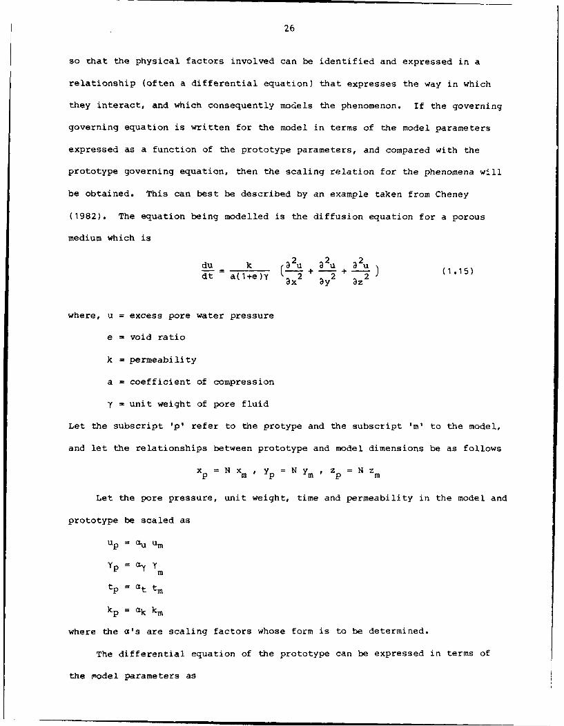
be obtained. This can best be described by an example taken from Cheney
(1982). The equation being modelled is the diffusion equation for a porous
medium which is
du k 2u u a 2 u
dt - a(1+e)y 3 + -- ;(2
where, u = excess pore water pressure
e = void ratio
k = permeability
a = coefficient of compression
y = unit weight of pore fluid
Let the subscript 'p' refer to the protype and the subscript 'i' to the model,
and let the relationships between prototype and model dimensions be as follows
xp =Nx yp = N ym , z = N z
Let the pore pressure, unit weight, time and permeability in the model and
prototype be scaled as
up = au um
Yp = acf Y
tp = at tim
kp = ak km
where the a's are scaling factors whose form is to be determined.
The differential equation of the prototype can be expressed in terms of
the model parameters as

27
aa u a k 2(a u 2( a u 2(a u )ur k m urn urn ur]
Da t = a(1+e) a y 2m 2(N )2 + + )2t x (ym )N (N zm m
a u t k m a a2u a2u a2u
ur km u m m ____
at tm a(1+e)a Y N2 a 2 2 2.
au at aka k a2u 2 2 um t U m m m
or21+ +
i.e at a a 2 a(1+e)y 2 2 m + m2m u y m ax ay am zm m m
au a~a k a2u a2u a2u
or -t- = 2 a(1+e) ym 2 2 2m Na m ma y am Zm
So, for similarity between the model and prototype equations,
= 1 (1.16)
N2 aY
Now k = - y where K is the physical permeability of the solid, y the unitn
weight of the pore fluid and n the pore fluid viscosity. Let the relationships
between the model and the prototype for the viscosity and physical
permeability be
np = ap n
K ypa K K m
Nowk = ak k =p p Ky m mp m TI a np r m
a K a
i.e. ak k = Y km a m
arK Lor ak = (.7
a

28
Substituting this value of ak in Equation 1.16, we get
aK a atKy- t
N2 -1
Y n
or K t2 - 1 (1.18)N2
N a
In centrifuge modelling of geotechnical prototypes involving soil, it is
usual to use the prototype soil in the model as the model soil then has the
same material properties as the prototype soil. Scale effects do not arise
unless, as previously discussed, the model is so small as to include only a few
grains of soil. Consequently, if, in the modelling of diffusion, the model and
prototype materials (solids and pore fluid) are the same, then
Kp = Km or aK = 1
and np = nm or an = 1
substituting these values of aK and an in equation 1.18, we get
t2 m 1at =N or -= N (1.19)
p N
In other words, if model dimensions are I times prototype dimensions, and ifN
both model and prototype materials are the same, then pore pressure dissipates
N2 times faster in the model when compared with the prototype.
Scott and Morgan (1977) provide a set of scaling relations which were
obtained with this approach. The only difficulty with this approach is that
ths governing equation of the phenomenon must be known. In some cases the
governing equation may be based on assumptions that may not be really
justified. In other cases, the phenomenon may be so complex that the

29
governing equation is not known. In such cases, the second approach, i.e.
dimensional analysis should be used.
1.5.2 Method Using Dimensional Analysis
This method is mcre general than the governing equation method and is used
where not enough is known about the prototype to formulate an equation that
describes its behavior. The method will be briefly explained in this section
with an example taken from Hoek (1965), showing how he modelled intact rock.
While the general theory is described in detail by Langhaar (1951), here the
basic procedure of dimensional analysis is summarized:
a) Identify the independent variables that play a role in determining
how the prototype behaves.
b) Arrange these independent variables to form dimensionless products.
c) Try and reproduce these dimensionless products in the model.
Thus the first step is to identify the variables involved. In order to do
this, enough must be known about the problem so that it is understood,
conceptually, whether and to what degree a variable influences the behavior.
Hoek (1965) analysed an elastic material in thermal equilibrium. His approach
was as follows: The behavior of a point in the structure, defined by coordinates
x, y and z, depends on the geometry of the structure, the material properties and
the applied force field.
Let the geometry of the structure be defined as
L = A typical length dimension, for example the diameter of a tunnel opening
rL = A set of dimensional ratios relating other dimensions of the structure to L.
Let the material properties of the prototype at this point (x, y, z) be
defined as
p - the density of the material
E - the Young's modulus of the material
v the Poisson's ratio of the material

30
The material properties at any point in the structure depend on the state of
stress, the direction of the bedding planes and, the material at that point.
Consequently, the material properties at various points in the structure may not
be the same as those at point x, y, z. If this is the case, then let the
properties at the various points be related to the properties at point x, y, z by
the set of dimensionless ratios rP, rE and rV.
The remaining area where similitude is required is in the applied stress
conditions. The stresses imposed on the model consist of those that are applied
externally, and those that are internal, such as a tectonic stress or a stress
due to gravitational body forces. Let the applied loads, stresses, displacements
and accelerations at point (x, y, z) be
Q = an externally applied load
P = an externally applied stress
ao = an internal stress, due for example to tectonic stress
g = an acceleration to which the entire body is subject to, and which results in
self-weight body forces
Uo = a displacement imposed directly on point x, y, z of the structure as
a result of a force
y = an acceleration imposed directly on point x, y, z of the structure.
The applied loads, stresses, displacements and accelerations at other points may
not be the same as those at point x, y, z. In this case, let them be related to
those at the point x, y, z by a set of dimensionless ratios rQ, rP , ro, rUO, ry.
Now, the displacement 'u' or the stress 'a' at point x, y, z is some
function of the above variables, i.e. they are each defined by some at present
unknown interaction among tae above variables. Thus,

31
u = f (x, y, z, t, L, p, E, Q, P, ao, g, v, v, rL, .... , rv) (1.20)
and
a = f (x, y, z, t, L, p, E, Q, P, a0 , g, v, V. rL, .... , rV) (1.21)
Each variable in the above functions has dimensions which are some
combination of the basic system of units, namely mass (M), length (L) and time
(t). By suitably arranging these terms, dimensionless products can be formed, as
follows.
a) Any dimensionless product iri can be written as
k I k2 k3 k4 k5 tk6 Fk7 k8 k9 pk10 Uk11 k12 k13 Qk14 k15ir.= u a x y z t F p g P o ao L .221. 0 0 ( .2
Many dimensionless products can be written from these variables, but only a few
will be independent of each other. By using the following procedure, a complete
set of dimensionless products can be obtained. A set of dimensionless products
of given variables is complete if each product in the set is independent of the
others in the set, and any other dimensionless product of the variables,
not in the set, is a product of powers of dimensionless products in the set.
b) Each variable can be written in terms of its basic dimensions as follows
a k2 M k2 Mk2 Ma2 k2
LT Lk 2 T2k2 Lb2k2 Tc2k2
Pk 8 M k 8 Mk8 Ma8 k8
L L 3k8 L 8 kS
32
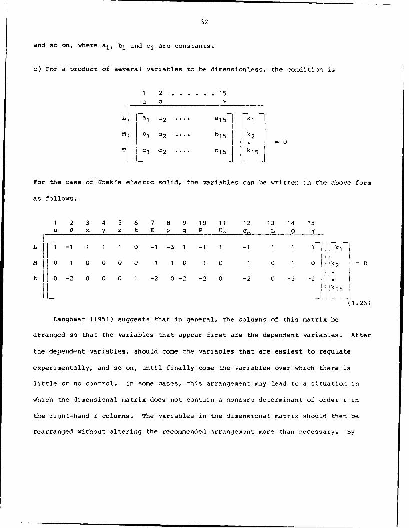
and so on, where ai, bi and ci are constants.
c) For a product of several variables to be dimensionless, the condition is
1 2 . . . . . . 15u a y
2 7a, a 2 .... al
M b, b2 .... b1 5 k2
T I c c2 .... c 1 5 - k1 5
For the case of Hoek's elastic solid, the variables can be written in the above form
as follows.
1 2 3 4 5 6 7 8 9 10 11 12 13 14 15u a x y z t E p g P U an L Q y
L 1 -1 1 1 1 0 -1 -3 1 -1 1 -1 1 1 1 k,
01 0 k2 = 0t 0-2 0 0 0 1 -2 0 -2 -2 0 -2 0 -2 -2
(1.23)
Langhaar (1951) suggests that in general, the columns of this matrix be
arranged so that the variables that appear first are the dependent variables. After
the dependent variables, should come the variables that are easiest to regulate
experimentally, and so on, until finally come the variables over which there is
little or no control. In some cases, this arrangement may lead to a situation in
which the dimensional matrix does not contain a nonzero determinant of order r in
the right-hand r columns. The variables in the dimensional matrix should then be
rearranged without altering the recommended arrangement more than necessary. By
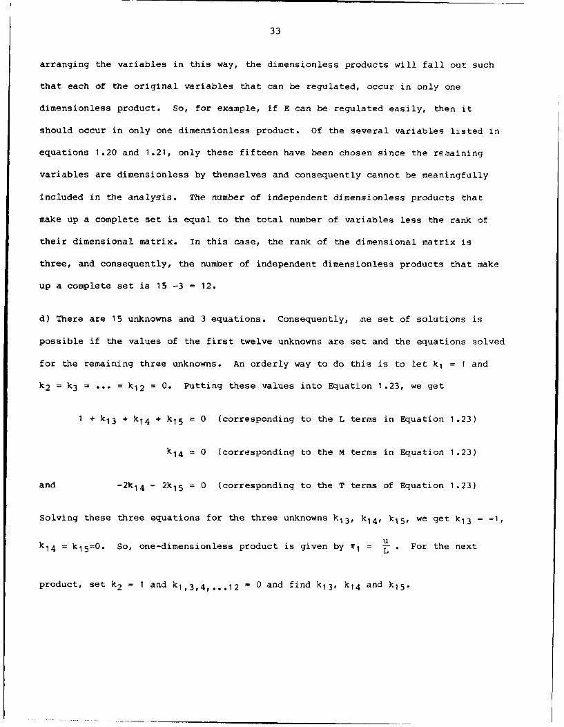
33
arranging the variables in this way, the dimensionless products will fall out such
that each of the original variables that can be regulated, occur in only one
dimensionless product. So, for example, if E can be regulated easily, then it
should occur in only one dimensionless product. Of the several variables listed in
equations 1.20 and 1.21, only these fifteen have been chosen since the renaining
variables are dimensionless by themselves and consequently cannot be meaningfully
included in the analysis. The number of independent dimensionless products that
make up a complete set is equal to the total number of variables less the rank of
their dimensional matrix. In this case, the rank of the dimensional matrix is
three, and consequently, the number of independent dimensionless products that make
up a complete set is 15 -3 = 12.
d) There are 15 unknowns and 3 equations. Consequently, ,ne set of solutions is
possible if the values of the first twelve unknowns are set and the equations solved
for the remaining three unknowns. An orderly way to do this is to let k, = I and
k2 = k3 = ... = k 12 = 0. Putting these values into Equation 1.23, we get
1 + k1 3 + k14 + k1 5 = 0 (corresponding to the L terms in Equation 1.23)
k14 = 0 (corresponding to the M terms in Equation 1.23)
and -2k14 - 2k15 = 0 (corresponding to the T terms of Equation 1.23)
Solving these three equations for the three unknowns k1 3 , k14 , k15, we get k1 3 = -1,
k14 = k50. So, one-dimensionless product is given by = Fortus " For the next
product, set k2 = I and ki, 3,4 ,...1 2 = 0 and find k1 3, k 14 and k15 .
34
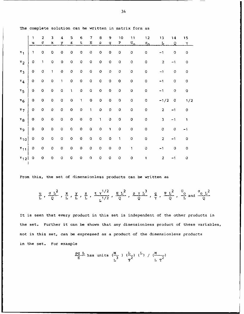
The complete solution can be written in matrix form as
1 2 3 4 5 6 7 8 9 10 11 12 13 14 15u a x y z t E p g P Un (O L Q y
7T1 1 0 0 0 0 0 0 0 0 0 0 0 -1 0 0
2 0 1 0 0 0 0 0 0 0 0 0 0 2 -1 0
ir 3 0 0 1 0 0 0 0 0 0 0 0 0 -1 0 0
IT4 0 0 0 1 0 0 0 0 0 0 0 0 -1 0 0
'T5 0 0 0 0 1 0 0 0 0 0 0 0 -1 0 0
It6 0 0 0 0 0 1 0 0 0 0 0 0 -1/2 0 1/2
#7 0 0 0 0 0 0 1 0 0 0 0 0 2 -1 0
#8 0 0 0 0 0 0 0 1 0 0 0 0 3 -1 1
It9 0 0 0 0 0 0 0 0 1 0 0 0 0 0 -1
ITo 0 0 0 0 0 0 0 0 0 1 0 0 2 -1 0
I11 0 0 0 0 0 0 0 0 0 0 1 0 -1 0 0
#121 0 0 0 0 0 0 0 0 0 0 0 1 2 -1 0
From this, the set of dimensionless products can be written as
a L2 1 t Yi/2 E L2 p y L3 g P L2 _ 0 Ua o L2u L I r z tyE yL g P and o
L' Q 'L ' L' L' 1/2 ' Q ' Q 'y' Q L QL
It is seen that every product in this set is independent of the other products in
the set. Further it can be shown that any dimensionless product of these variables,
not in this set, can be expressed as a product of the dimensionless products
in the set. For example
pg_L h s u i s ( ) ) (L) / (M_ ).2has uni ts M L L M
L T LT

35
or is dimensionless. However, it can also be expressed in terms of the previous
dimensional products. i.e.
pq L P YL g QE - Q Y E L 2
In other words, the set of dimensionless products that has been obtained is
complete, since it satisfies the definition of --ompleteness.
As stated before, the displacement 'u' and the stress 'a' at points x, y, z can
be expressed as functions of all the variables involved as in equations 1.20 and
1.21, namely,
u = f(x, y, z, t, L, p, E, Q, P, a0, g, v, rL, ... rV) (1.20)
and a = f' (x, y, z, t, L, p, E, Q, p, ao r g, v, rL ... rV) (1.21)
Buckingham's Theorem (also called the 7 theorem) states that if an equation is
homogenous, it can be reduced to a relationship among a complete set of
dimensionless products. In other words, displacement u or stress a, in the form of
a dimensionless product, can be related to all the other variables when expressed
as a complete set of dimensionless products. Using the complete set just
obtained, the following relations result.
1/2 t L2 PYL 3 PL 2 U L2 L E,u F [ x fy .z .t Y v, r , Lr oL EL L L L' 1/2' Q L L, Q ,vrrL
rV, rQ, rp , rU , r P, r a ry] (1.24)
and
aL2F , .... (. 25)
where F and F' are functions expressing the relation among the dimensionle<- terms.
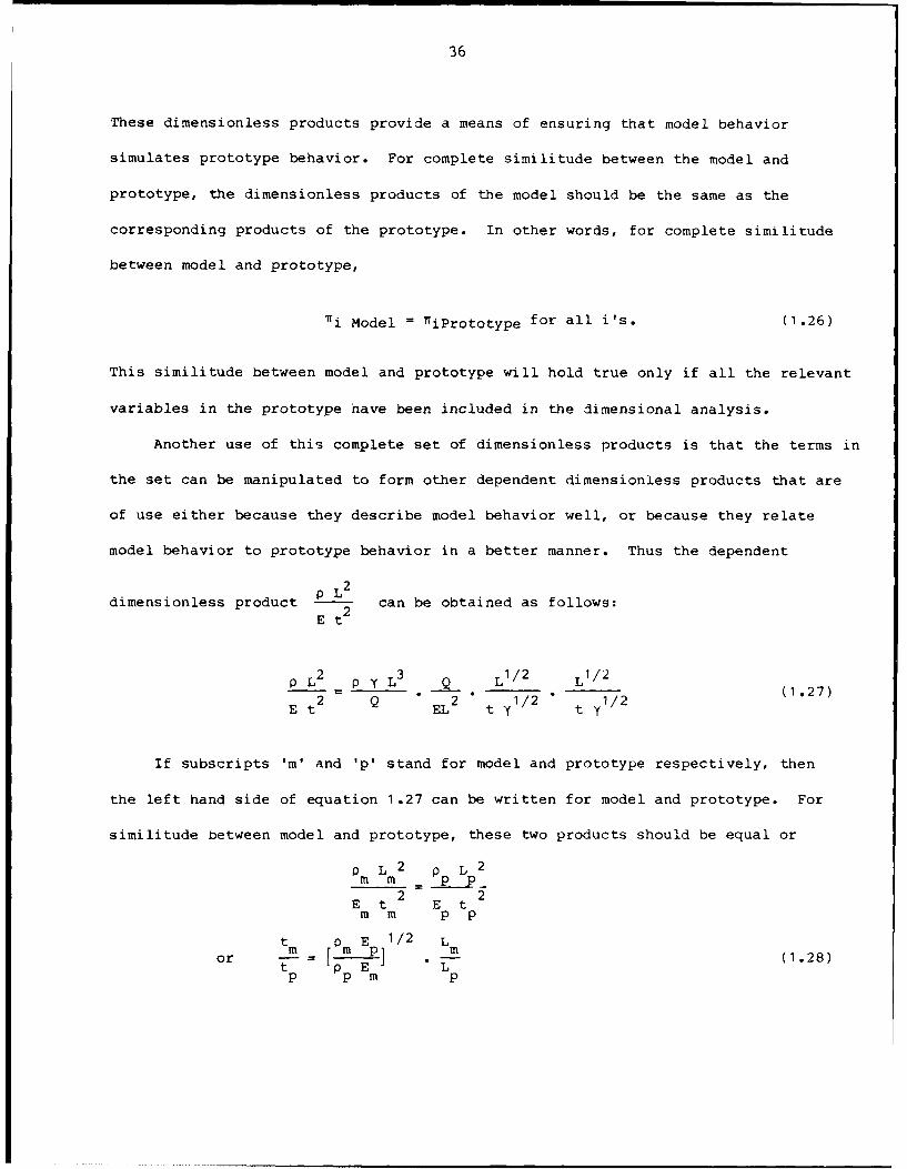
36
These dimensionless products provide a means of ensuring that model behavior
simulates prototype behavior. For complete similitude between the model and
prototype, the dimensionless products of the model should be the same as the
corresponding products of the prototype. In other words, for complete similitude
between model and prototype,
ffi Model = riPrototype for all i's. (1.26)
This similitude between model and prototype will hold true only if all the relevant
variables in the prototype have been included in the dimensional analysis.
Another use of this complete set of dimensionless products is that the terms in
the set can be manipulated to form other dependent dimensionless products that are
of use either because they describe model behavior well, or because they relate
model behavior to prototype behavior in a better manner. Thus the dependent
pL 2
dimensionless product can be obtained as follows:E t
2
p L p Y L Q L1/ 2 L11 2
2 Q EL2 1/2 1/2 (1.27
If subscripts 'im' and 'p' stand for model and prototype respectively, then
the left hand side of equation 1.27 can be written for model and prototype. For
similitude oetween model and prototype, these two products should be equal or
Pm Lm 2 pp Lp2
E 2 2E t E tm m p p
t P E 1/2 Lor (1.28)
p p m p

37
i.e. by manipulating the independent dimensionless products a dependent product has
been obtained which expresses the scaling relationship foL time between the model
and the prototype in terms of the respective material properties and lengths.
Dimensional analysis is a powerful tool in modelling. For example, it does
not matter if Ep is not equal to Em, as long as the dimensionless products that
E L2
contain Ep and Em are equal, i.e., - is the same for both model and prototype.
Perhaps the most important part of the analysis is the identification of the
relevant independent variables. Once the independent variables have been identified
and the dimensionless products formed, then every attempt is made to reproduce the
values of these dimensionless products in the model. Complete similitude is usually
not possible, in which case variables whose effects are minor are allowed to deviate
from their theoretically correct values. If the effect of a variable is fully
known, and, its scaled value is not reproduceable in the model, then the variable is
allowed to depart from its correct value, and a correction is later made for its
effect on the results. Once equality of the dimensionless products is achieved,
then by equating the dimensionless products of the prototype to those of the model,
scaling relationships such as the scaling relationship given by equation 1.28 can be
obtained.
1.5.3 Scaling Relationships
This section establishes various basic scaling relationships, deriving them
from first principles, for the case of a model subject to Ng in the centrifuge, and
made up of the same material as the prototype. As noted previously, either the
governing equation approach or the dimensional analysis approach or both can be used
to obtain the relationships. The derivations of the scaling relationships are given
in the subsequent sections and are su marized in Table 1.1.

38
Table 1.1
Model Dimension
Equation Number Quantity Symbol Prototype Dimension
1 For All Events
1,29 Length L
1.29 Displacement U -
1.30 Area A 1
N2
1.31 Volume V 1N3
1
1.32 Mass M 3N3
1.33 Density P 1
1.34 Strain
1.35 Force F 2N
1.36 Stress a
1
1.37 Energy -- 3N
1.38 Energy Density i

39
2. For Dynamic Events
1.39 Acceleration a N
11.40 Time t
N
1.41 Velocity v1
1.42 Frequency N
1.43 Strain Rate ; N
3. For Self Weight
1.44 Acceleration a N
4. For Diffusion Events
1.45 Time t 1
12
1.46 Velocity v N
1.47 Acceleration a N3
1.48 Strain Rate e N2
5. For the Laminar Flow of Water Through Soil
1.49 Permeability k N
1.50 Head LN
1.51 Pressure p 1
1.52 Hydraulic i 1Gradient
1.53 Velocity v N
1.54 Flow Quantity Q 1

40
1.56 Capillary Rise D 1N
1
1.57 Time t 2N
6. For Viscous Effects
1.35 Force F
N2
1.59 Time t
1.60 Velocity v N
11.61 Acceleration a1
N

41
1. For All Events
For a model rotated at Ng, in order to satisfy the condition of geometric
similarity with the prototype, it is required that lengths L and displacements U be
scaled as follows
L Um m 1. . . . . (1 .29)
L U NP p
Now area A has dimensions L2 and so scales as
A L 2m m 1. = . . ( 1 . 3 0 )
Ap L 2 N2
p
V L3
and volume V as - m __a 1 (1.31)V 3 N3p L N
P
M PmL 3m mm
Mass = PL3 , scales as m - - (1.32)M 3 3P PpLp N
Density by definition is independent of g and so
-=1 (1.33)pp

42
Strain C scales as
ALmL AL L
x - - . N = 1 (1.34)6 AL AL L Np p p m
Lp
F M gFm m - 1 1Force =F scales as -N =- (1.35)F p p gp N3 N2
F F /A 1 2Consequently stress a scales as .- . N 1 (1.36)p Fp/Ap 2
1I m M sm g m hp 1 I
Potential energy n scales as p gm h 33 1 1 (1.37)
Energy density n is energy/unit volume and scales as
M Mgm hm/L3mmn = n i n i 1 1 N3. . gh-.. N =1 (1.38)p Mp gp hp/Lp3 N3 N
2. For Dynamic Events
The inertia force F = Ma and scales as
F M a
F Map pp
From 1.35 we know that any force scales as - .Also from 1.32 we know thatFp N2
M
3 Substituting for F and M in the scaling relation for force, we getp N
a-- = N (1 .39)ap

43
a L t -2 t 2
Now m m P = Na -2 N 2p L t t
p p m
t 2 tioe. tP 2 tm 1
- N or - = - (1.40)2 t N
t p
V L tVelocity V scales as V - 1 M " N = 1 (1.41)
p L t
p pptfAs t N -' it follows that frequency f scales as - N (1.42)
p p
in order to maintain the same number of cycles in the model per unit of prototype
time.
Strain rate £ scales as
ALm
£ L t AL L t= En m p _ • N . N N (1.43)
- -AL TL L t Np p p m m
L tp p
3. For Self Weight
Acceleration on the model is increased to Ng by controlling the rotational
speed of the centrifuge so that w2R = Ng and
aN (1.44)
ap
44
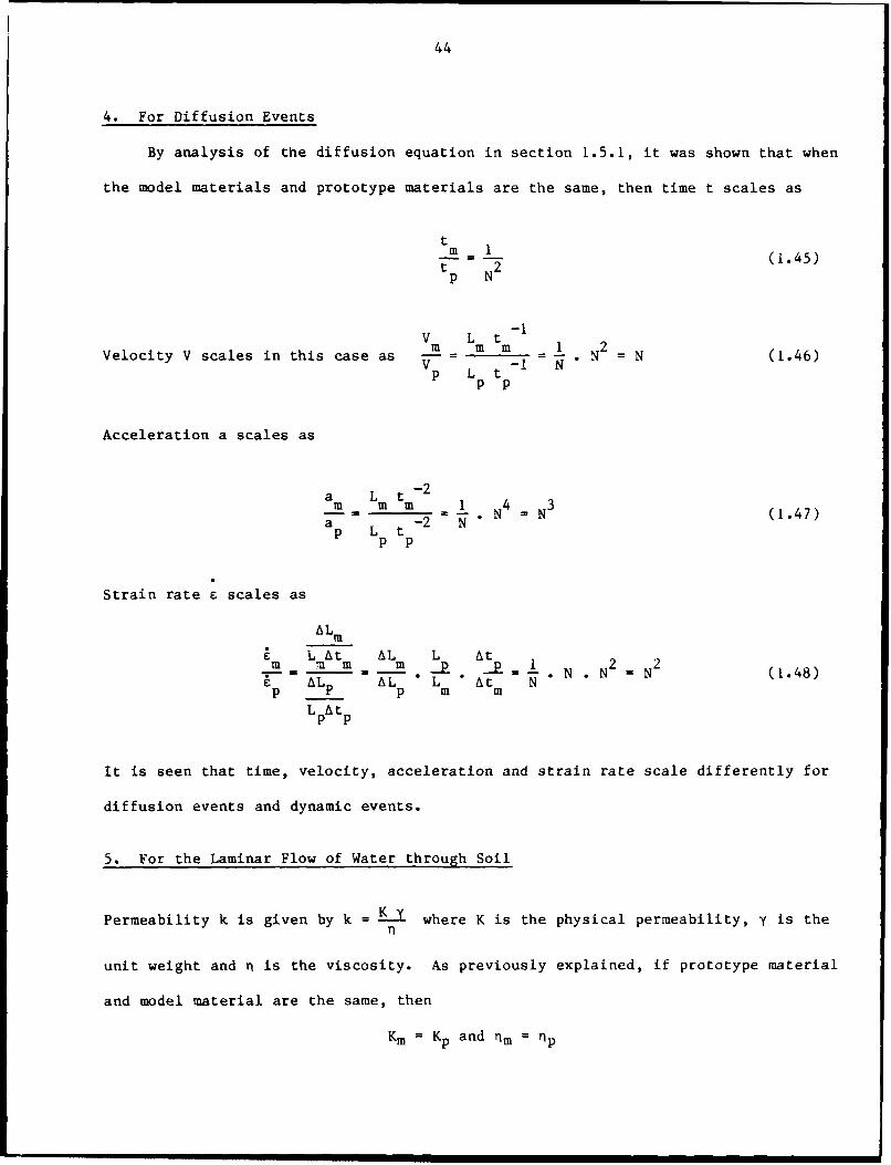
4. For Diffusion Events
By analysis of the diffusion equation in section 1.5.1, it was shown that when
the model materials and prototype materials are the same, then time t scales as
ttn- (1.45)tp N2
V L tm m m 1 N2Velocity V scales in this case as N - N * N - N (1.46)
p L t
Acceleration a scales as
a L t 4 3
m = . =N (1.47)a -2 Np L t
Strain rate ; scales as
ALM
L At AL L Atn- __. .-. i . N 2 (1.48)g AL AL *L At Np Pp m in
L pAtLptp
It is seen that time, velocity, acceleration and strain rate scale differently for
diffusion events and dynamic events.
5. For the Laminar Flow of Water through Soil
Permeability k is given by k =EK where K is the physical permeability, y is the
n
unit weight and n is the viscosity. As previously explained, if prototype material
and model material are the same, then
Km = Kp and nm= np
45
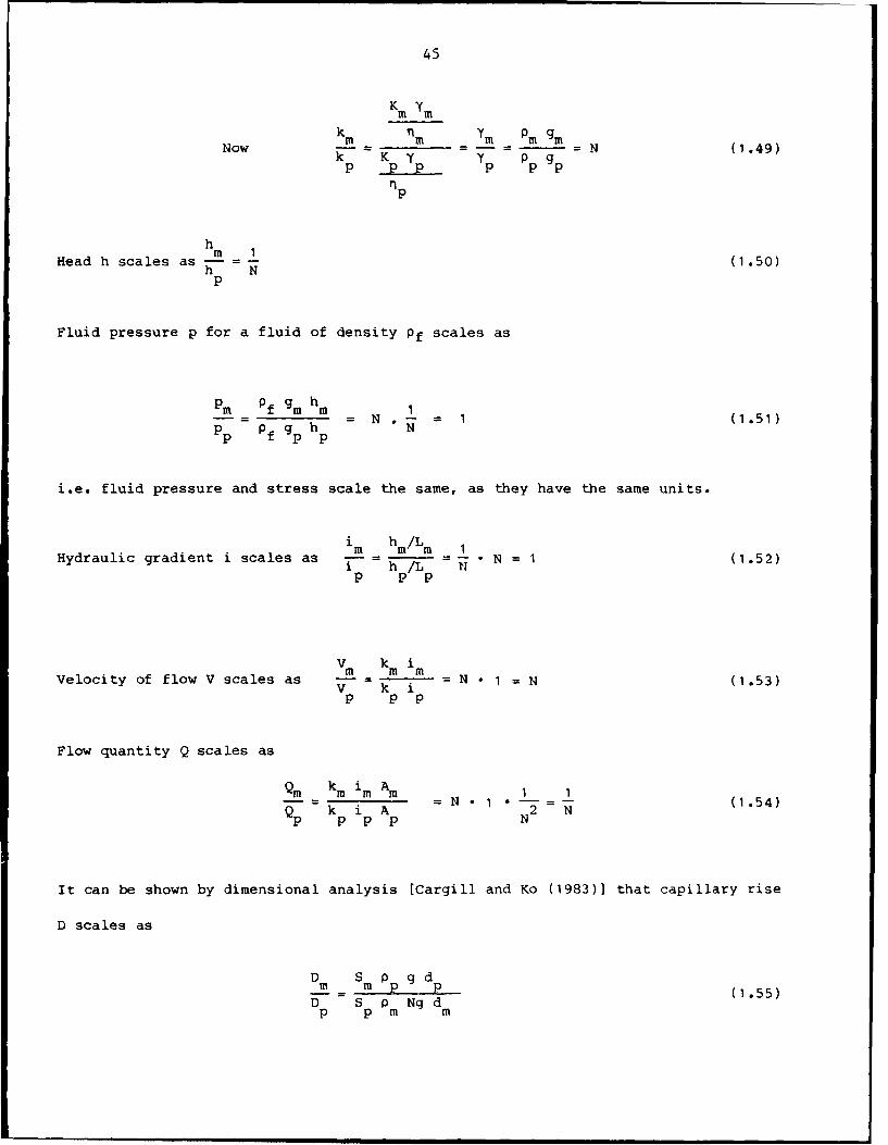
Km Ymm m m m
Now __M = = =N (1.49)k K p Yp pp pP 1 P
hm 1Head h scales as h = N (1.50)
p
Fluid pressure p for a fluid of density Pf scales as
Pm Pf gm h1m- N . - 1 (1.51)pp pf gph N
i.e. fluid pressure and stress scale the same, as they have the same units.
i m hm/Lm 1Hydraulic gradient i scales as i h /L = N = 1 (1.52)
V k im m mVelocity of flow V scales as V= k = N 1 1 = N (1.53)
p P p
Flow quantity Q scales as
Qm km im Am 1 1N 2 - (1.54)
Qp kpp ip Ap N2 N
It can be shown by dimensional analysis [Cargill and Ko (1983)] that capillary rise
D scales as
0 S ppg dm Sm P p (1 .55)
D p S pm Ng dm

46
where S is the surface tension and d is the effective diameter of the inter-particle
voids. Since model and prototype are made of the same material, p = Pm, dp = dm
and Sp = Sm so that
Dm 1D =N- (1.56)D Np
1
In a model, the distance between two points is I times the distance between two
geometrically similar points in the prototype. Further, the velocity of flow in the
model is N times the velocity of flow in the prototype (equation 1.53). Pokrovsky
and Fyodorov (1936) predicted that because of this time would scale as
t m 1= - (1.57)
tp N2
6. Viscous Effects
The viscous force 'F' acting on a small area 'A' can be defined as
F = ,s - A , (1.58)s dn
where Ps is the viscosity of the soil skeleton, and dv is the differential
of the soil velocity with respect to the normal 'n' to the flow direction. Hence
Fm Usm dVm dn Am
F 11 .dn *Ap sp p m p
Viscosity p is independent of gravity and so, for the same material in the
model and prototype, 1sm = sp" Consequently, the drag force scales as
F M dV dn Am
F dV dn *Ap p m p
-1L t L L
m m p m-1 L L2
L t m p
t -1m 1
t Np

47
Since any force scales as 1 for the viscous force one obtainsN2
-1t1 m 1
2- N or,N 2 t 1 N2
p
tm-- 1 (1.59)
p
-1
V L t 1 1Velocity V scales as -1 N N N (1.60)
p L tPp
Acceleration 'a' scales as
-2a L tm m m 1 1 1 (1.61)a -2 N Np L t
The various scaling relations that have been derived are shown in Table 1.1.
1.5.4 Discussion of Scaling Relationships
The scaling relations described in the previous section are valid only if the
model and prototype materials are the same. On examining the scaling relationships,
it is clear that it may not be possible to satisfy all the similitude requirements,
leading to possibly significant errors, especially at high values of the model
factor 'N'. A number of cases are possible:

48
One case is where two or more parameters with conflicting scaling relations
play a significant role in the phenomenon being modelled. An example of this
situation would be the case of modelling ice-structure interaction, where both
velocity and strain rate play a role. From the previous section it is seen that for
dynamic events, velocity scales at 1:I (model: prototype), while strain rate scales
at N:1. Now the strength of ice is significantly strain rate dependent, while the
forces exerted on the ice flow are functions of the velocity of movement.
Consequently, if the velocity is scaled correctly, then the model strain rate is N
times the prototype strain rate. In this case one solution is to model the
velocity, and, knowing the strength of the model ice at the resulting model strain
rate, input these values into a theoretical model and check to see if the results
from the theoretical model correspond with the results from the centrifuge tests
[Vinson (1982)].
The second case is when the same parameter or variable has a different scaling
relationship depending on the process with which it is associated and two or more
such processes occur within the same phenomenon. A classic example of this is
liquefaction. The initial part of the phenomenon - the collapse of the soil
structure and the generation of pore pressures - is associated with dynamic shaking
while the latter part - the dissipation of the excess pore pressure - is a diffusion
tm 1type process. For a dynamic event, time scales as - = - , while for the case of
p
t m Idiffusion, time scales as 2- . Often, in such cases the approach used would
p N
be to model the two processes separately. Thus the time scale for the initial
tm Iportion of the phenomenon i.e. till liquefaction occurs, is - = , while the
t Np
time scale for the subsequent dissipation of excess pore pressure is i . Tan andN
49
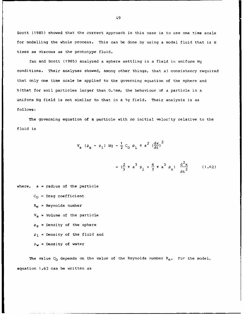
Scott (1985) showed that the correct approach in this case is to use one time scale
for modelling the whole process. This can be done by using a model fluid that is N
times as viscous as the prototype fluid.
ran and Scott (1985) analyzed a sphere settling in a field in uniform Ng
conditions. Their analyses showed, among other things, that a) consistency required
that only one time scale be applied to the governing equation of the sphere dnd
b)that for soil particles larger than 0.1mm, the behaviour of a particle in a
uniform Ng field is not similar to that in a Ig field. Their analysis is as
follows:
The governing equation of a particle with no initial velocity relative to the
fluid is
V g - 2 d x 2Vs (Ps - Pl) Ng PI D d)
d22 3 4 3 )dx ( .2= (7 T a p1 + n i a p (1.62)
3 1 3 2t
where, a = radius of the particle
CD = Drag coefficient
Re = Reynolds number
Vs = Volume of the particle
Ps = Density of the sphere
Pl = Density of the fluid and
Pw = Density of water
The value CD depends on the value of the Reynolds number Re. For the model,
equation 1.62 can be written as

50
dx 2 d2xA Ng + (CD ) B( dt M) = C 2 m (1.63)
m m dtm
where A = V (p - p ) B and,s s 2 1
C = 2 IT a3 (P + 2ps) and 'have the same values as in the prototype.3 1 s
For the prototype, N = 1 and the corresponding equation is
dx 2 d2xAg + (C) B(d) = C p (1.64)
D dt dt 2p p dpt
1m I Xp
For the model, - or x -
x N m Np
Substituting this in equation 1.63, and dividing by N, gives
1 dx 2 d~x
Ag + (C) 1 1 dB) 2= C 2 p (1.65)D N3 (dt N2 dt2m N m N dt
in
For no fluid, CD = 0 or B = 0 and equations 1.64 and 1.65 reduce to
d2xAg = C (1.64a)
dt2
p
and 2C d x
Ag N - (1 .65a)N 2dt2m
Consequently, for similitude between Equations 1.64a and 1.65a, t 1 t (1.66)m Np

51
For the case with a fluid, CD * 0 and B * 0, and similitude between model and
prototype requires equations 1.64 and 1.65 to be equivalent. For them to be
equivalent, the following conditions should be met
t = 1 t (1.67)m N p
and (CD)m = N(CD)p (1.68)
For low Reynolds number (Re < 1.0),2Pla dx
R = (1.69)e 0 dt
and C =24 2 (1.70)D Re 2pla dx/dt
where v is the fluid viscosity.
dx Ndx dxUsing equation 1.67, p - m _ m (1.71)
dt Ndt dtp m m
Substituting equation 1.70 in equations 1.64 and 1.65, the following equations are
obtained.
From equation 1.64 (Prototype),
dx d2x24B p P (1.72)
p 2pda dt 2p dtp
and from Equation 1.65 (Model), with t = tm N p
dx d~x1m 24B px dp
A g + = C- (1.73)N 2Pla dtp d t 2
P
52
So, for Equation 1.73, which represents conditions in the model, to be identical with
Equation 1.72, which represents conditions in the prototype, um should be equal to
N Up. When pm = N Up., the phenomena in the model will be the same as in the prototypetm 1
with time scaling as - = - . A glycerine-water mixture or silicone oil can be usedt Np
to obtain the required viscosity, while at the same time, a correction must be made to
account for any difference in densities. Further, when Re in the prototype exceeds 1,
then the drag force is no longer a linear function of velocity in the prototype.
In the model however, since Um = N up the correspondingly scaled Re for the model
(Re)pis N , which may be less than 1 up to the terminal velocity. Consequently the drag
force on the particle in the centrifuge at Ng will be a linear function of the
velocity and there will no longer be similitude between the model and the prototype.
In other words, behavior at Ng in the model need not be the same as behavior at Ig in
the prototype.
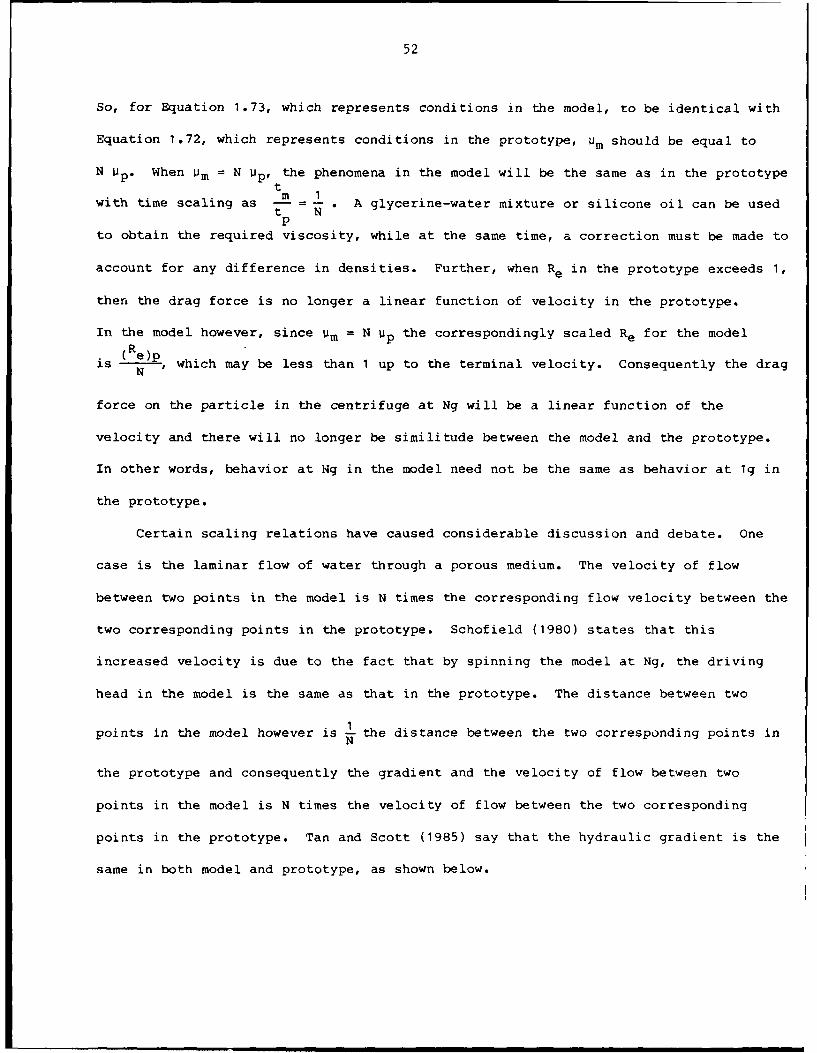
Certain scaling relations have caused considerable discussion and debate. One
case is the laminar flow of water through a porous medium. The velocity of flow
between two points in the model is N times the corresponding flow velocity between the
two corresponding points in the prototype. Schofield (1980) states that this
increased velocity is due to the fact that by spinning the model at Ng, the driving
head in the model is the same as that in the prototype. The distance between two
1points in the model however is I the distance between the two corresponding points in
the prototype and consequently the gradient and the velocity of flow between two
points in the model is N times the velocity of flow between the two corresponding
points in the prototype. Tan and Scott (1985) say that the hydraulic gradient is the
same in both model and prototype, as shown below.

53
At Ig in the model,
1 1h = - h and x x
in N p m N pmig mig
At Ng,
h = h and x = xmNg P mNg p
And consequently
m 8= Ng = p P (1.74)
m ax -Nx pmNg
They attribute the change in velocity to the fact that the permeability k is not a
material constant, but since it is defined ask = y _ _ K
it depends on the unit weight y and consequently on the g field, i.e. permeability
scales as
k ym k yp Km m p- =----- /k U 1 /
p m p
Now, if the same materials are used in the model and prototype, then
Um = Up 'K m =Kp and ym =N yp
or
km YM PM gmk - - p -N (1.75)
kp Yp Pp 9p
i.e. km = N kp and consequently
Vm = km im = N kp ip = N Vp. (1.76
Note that this derivation is exactly the same as that given in section 1.5.3, under
laminar flow of water through soil.

54
Goodings (1984) says that some researchers prefer to consider Darcy's
coefficient of permeability, k, as a material constant since in the normal
geotechnical context, a change in k, implies a change in the material structure.
From this view point, the increase in self-weight must be reflected by a
corresponding increase in hydraulic gradient. This increased hydraulic gradient is
argued for on the basis that the rate of loss of water pressure occurs at a rate N
times faster in the centrifuge model.
Tan and Scott (1985) have shown clearly that k is not a material constant, but
changes with the unit weight of the permeant. Further, consistent applications of
the scaling laws shows that the hydraulic gradients in both model and prototype are
Lie same. Consequently, it appears that the arguments presented by Tan and Scott
(1985), are more correct. However, regardless of the reason, it is commonly
accepted that the velocity of the flow in the model is N times the corresponding
flow velocity in the prototype. Consequently, flow that is laminar in the
prototype, could be turbulent in the model.
Once the model and the scaling relations have been chosen, it is desirable,
that in view of the above uncerta .ties, a check be run to see if behavior similar
to that of the prototype is obtained. Prototype behavior however is not known, and
further, extrapolation of results to prototype dimensions may not be justified. In such
cases, the technique of 'modeling of models', which was previously described, is used.
1 1If the results of a 1 scale model tested at 100g are the same as those of a -
model run at 20g, then one can conclude with reasonable justification that these
results are also represensative of the unscaled model at 1g. This modeling of
models' technique establishes the 'internal consistency of the experiment' or the
range within which the scaling relations apply.

55
Rather than viewing a test as modelling a prototype, a test may be
viewed as a real event in itself, with no attempt being made to simulate any exact
prototype condition. Theories, which can be later applied to lg situations, can be
tested on these real events. Finally, a possibility exists that some feature of the
prototype is too complex to be exactly scaled. In ice-structure interaction problems
for example, it may not be possible to model the complex arctic ice structure. One way
that has been suggested (Vinson (1982)] is to apply a correction, to the results of
centrifuge tests, which analytically accounts for the more complex structure of the
arctic ice.
1.6 Summary
This section summarizes the problems that may be encountered in centrifuge
testing and methods that are of use in correcting for them. The problems can be
classified in two general categories - problems associated with the centrifuge
and problems associated with scaling.
Problems associated with the centrifuge are discussed in section 1.2.3. The ideal
gravity field for modeling is an Ng field whose magnitude and direction does not change
from point to point. In the centrifuge, the g field varies linearly with depth and,
consequently, the effective stresses vary parabolically through the model depth in
contrast with the prototype where the variation is linear. The difference in stresses
generally being less than 2%, it is neglected.
The centrifuge gravity field acts radially and so if the model surface is not
curved to the centrifuge radius, then the model stresses at two points at the same
depth will not be the same, but the difference being less than the difference due to
the first error (parabolic as opposed to linear stress variation) it is neglected.
Since the acceleration field acts radially, there exists a horizontal component of
acceleration that could be significant in some problems, e.g. slope stability, and
consequently should be considered. Finally, improper orientation of the platform and

56
also the time required to reach the desired g level may also cause minor errors, but
these errors can be corrected for.
Successful centrifuge testing requires that the scaling relations between the
model and prototype be understood and satisfied. Successful testing also requires
that the model behave at Ng as the prototype behaves at 1g. Scaling relations were
examined in detail and it was shown that if the governing equation of the phenomenon
is known, these relations can be obtained from the equation. If the governing
equation is not known, however, then the more general method of dimensional analysis
can be used. The success of this method depends on correctly chosing the independent
variables, which in turn requires at least some understanding of the problem. Using
either of these methods, a number of basic scaling relations were obtained for various
situations, in each of which the model material was the same as the rototype
material. Exact scaling of a phenomenon is sometimes not possible, as the various
prototype features may be difficult to model.
In conclusion, the centrifuge is a useful tool, and if properly used, can provide
useful information about the prototype.

57
2. Geotechnical Applications of the Centrifuge
2.1 Introduction
Centrifuge research in geotechnical engineering encompasses many areas, notably,
soil mechanics, rock mechanics, ice mechanics and gravity tectonics. This section
provides an overview of the research that has been performed in these areas and
gives an idea of the breadth of research that is possible using the centrifuge. In
the sections on soil, ice and gravity tectonics, only a brief review of the
research done is presented. whereas, more details are provided for work done in the
area of rock mechanics. Most of the recent geotechnical work that has been done on
the centrifuge deals with soil models, while relatively little work has been done in
the remaining areas, the reason being that soil lends itself more easily to
centrifuge testing rather than rock, ice, or models of tectonic structures.
2.2 Soil Mechanics
This section summarizes work that has been done in soil mechanics, with the
centrifuge. Since a relatively large amount of work has been done, it is described
under the following headings: Flow of Water Through Soils, Soil-Structure
Interaction, Underground Construction, Dynamics and Miscellaneous.
2.2.1 Flow of Water Through Soils
Many geotechnical problems involve water movement through or on soil. The
problems fall into the following broad categories: a) Steady flow of water through
soils; b) Diffusion of excess pore water pressure; c) Erosion, river basin flooding,
and similar problems. Liquefaction though involving water is treated under the
section on dynamics.
The steady flow of water through soils is central to the study of many
geotechnical problems involving seepage. The flow of water may be either laminar or
turbulent. Many researchers have worked on laminar flow and have derived the
58
scaling laws required for modeling, for example: Laut (1975), Goodings (1979),
(1984), Cargill and Ko (1983), etc. The phreatic surface for steady state seepage
through homogenous embankment dams for laminar flow has been successfully modeled by
Goodings (1979). Turbulent seepage horwever does not appear to have been modeled on
the centrifuge, though Goodings (1984) has derived the appropriate scaling
relations. She, however, says that the validity of some of the equations on
which these scaling relations are based have not been established at 1g.
The diffusion of excess pore pressure has been successfully modeled in the
centrifuge by Croce et al (1984) who modeled the self-weight consolidation of a
thick layer of soft clay, using the centrifuge. They were able to verify the scalingt m I
relations for diffusion, including the scaling for time, i.e. - =
p N
By comparing centrifuge test results with various theories, they showed that
conventional small strain consolidation theory was inadequate for studying the
self-weight behavior of soft clays, but that finite strain consolidation theory
provided an accurate prediction of prototype response.
Various other problems involving the interaction of water and soil have been
studied. Padfield and Schofield (1983) modeled a flood embankment made of clay and
built on a clay foundation layer which in turn overlay a pervious gravel layer. By
applying high water pressures to the pervious layer, they simulated high uplift
pressures on the embankment, and were able to model the failure process. In another
similar study, Schofield (1980) modeled underwater flow slides that occur as a
result of erosion of the underlying clay layers, and proposed a failure hypothesis
based on the test results.
2.2.2 Soil-Structure Interaction
The centrifuge has been extensively used to study soil-structure interaction
problems. This section lists some of the major areas that have been studied.

59
The centrifuge at the Peter W. Rowe Laboratory at the University of Manchester,
England, has been used extensively to study coastal and offshore gravity structures.
Model studies were conducted for the design of the Oosterschelde storm surge barrier
in the Netherlands. A field model experiment was undertaken at one-third full scale
and both this experiment and the projected prototype were modeled in a series of
centrifuge experiments (Rowe and Craig (1976)]. The centrifuge tests gave realistic
results. Rowe and Craig (1978) later studied the effect of variations in weight and
shape of the structure. George and Shaw (1976) and Rowe and Craig (1980) also
investigated the stability of an already designed concrete gravity structure to be
placed in a gas field in the North Sea. Failures by surface sliding and/or
associated shakedown settlements were reported by Rowe (1975) when the prevalent
analyses assumed deep seated failure mechanisms. Centrifuge tests have consistently
shown that whether founded on cohesionless soil, on cohesive soil or on mixed
strata, the failure of models under cyclic loading has always been observed at or
close to the mudline on essentially flat-bottomed structures [Rowe and Craig (1980)],
or close to the level of the tips of surface penetrating skirts [Craig and Al-Saodi
(1981)].
In America, Prevost et al (1981) used the technique to study foundations of
off-shore gravity structures. A model off-shore platform was machined out of aluminum
and sand glued to its bearing surface, to simulate in-situ conditions. As in the
prototype, the model was provided with skirts. Vertical and horizontal loads were
applied, and the resulting movements measured. The effect of cyclic loads on the
platform was also studied. Prevost et al (1981) concluded that centrifuge simulation
was possible and suggested that further experiments be ran to assess the reliability
of alternative design or analysis techniques.

60
Scott (1971a, 1979b, 1981) did a considerable amount of centrifugal testing of
piles in sands. He investigated the behavior of piles subject to cyclic loading.
Discrepancies were observed between field and model tests, which were attributed to
the fact that the piles were not driven under field stress conditions and that,
consequently, the sand around the model pile was not as dense as the sand around the
prototype pile. Sabagh (1984) ran cyclic axial load tests in piles in sand and
found that the magnitude of cyclic load at failure was controlled by the existing
static load, the size of the load increment and the number of cycles. Oldham (1984)
investigated the lateral loading of single piles in sand. To model field
conditions, he drove the piles in flight. The load-deflection curve showed
reasonable agreement with published field values, though the experimental values
showed slightly more flexible behavior ii the initial part of the load deflection
curve, as compared to field behavior. Finn et al (1984) studied the dynamic lateral
response of pile foundations and found that their numerical technique gave adequate
information for design for seismic loads. Nunez and Randolph (1984) modeled tension
piles in soft clay. Instrumented piles of various flexibilities were driven in
flight into carefully prepared clay samples. Craig (1984), did installation studies
for model piles and concluded that it may not be possible to simulate pile group
installation in the centrifuge. Barton (1984) studied the response of pile groups
to lateral loading. From the various test programs done on piles, it can be
concluded that accurate modeling requires that the piles be driven in flight to
simulate field conditions. This makes successful instrumentation of the model pile
difficult. Once the instrumented pile is driven in sand or clay, then its behavior
can be studied using various loading mechanisms. Modeling pile groups, however, is
not straightforward, due to interaction effects between individual piles.
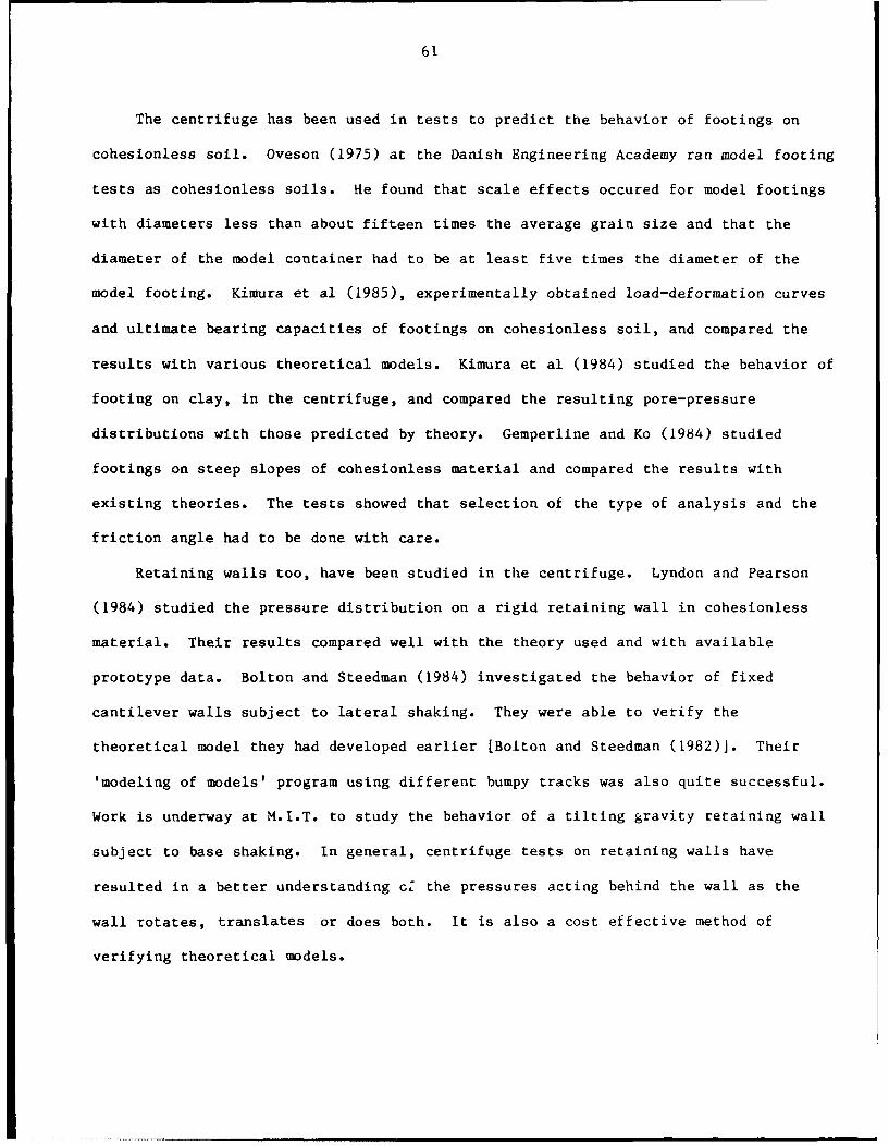
61
The centrifuge has been used in tests to predict the behavior of footings on
cohesionless soil. Oveson (1975) at the Danish Engineering Academy ran model footing
tests as cohesionless soils. He found that scale effects occured for model footings
with diameters less than about fifteen times the average grain size and that the
diameter of the model container had to be at least five times the diameter of the
model footing. Kimura et al (1985), experimentally obtained load-deformation curves
and ultimate bearing capacities of footings on cohesionless soil, and compared the
results with various theoretical models. Kimura et al (1984) studied the behavior of
footing on clay, in the centrifuge, and compared the resulting pore-pressure
distributions with those predicted by theory. Gemperline and Ko (1984) studied
footings on steep slopes of cohesionless material and compared the results with
existing theories. The tests showed that selection of the type of analysis and the
friction angle had to be done with care.
Retaining walls too, have been studied in the centrifuge. Lyndon and Pearson
(1984) studied the pressure distribution on a rigid retaining wall in cohesionless
material. Their results compared well with the theory used and with available
prototype data. Bolton and Steedman (1984) investigated the behavior of fixed
cantilever walls subject to lateral shaking. They were able to verify the
theoretical model they had developed earlier [Boiton and Steedman (1982)]. Their
'modeling of models' program using different bumpy tracks was also quite successful.
Work is underway at M.I.T. to study the behavior of a tilting gravity retaining wall
subject to base shaking. In general, centrifuge tests on retaining walls have
resulted in a better understanding Gf the pressures acting behind the wall as the
wall rotates, translates or does both. It is also a cost effective method of
verifying theoretical models.
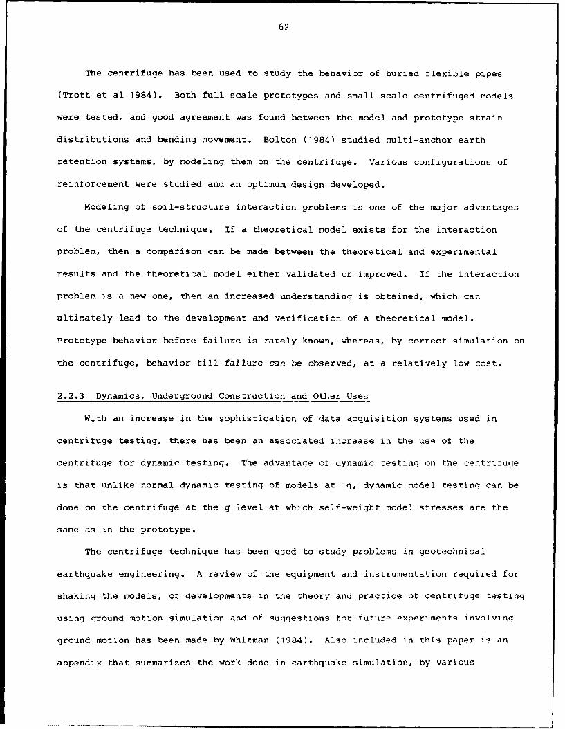
62
The centrifuge has been used to study the behavior of buried flexible pipes
(Trott et al 1984). Both full scale prototypes and small scale centrifuged models
were tested, and good agreement was found between the model and prototype strain
distributions and bending movement. Bolton (1984) studied multi-anchor earth
retention systems, by modeling them on the centrifuge. Various configurations of
reinforcement were studied and an optimum design developed.
Modeling of soil-structure interaction problems is one of the major advantages
of the centrifuge technique. If a theoretical model exists for the interaction
problem, then a comparison can be made between the theoretical and experimental
results and the theoretical model either validated or improved. If the interaction
problem is a new one, then an increased understanding is obtained, which can
ultimately lead to the development and verification of a theoretical model.
Prototype behavior before failure is rarely known, whereas, by correct simulation on
the centrifuge, behavior till failure can be observed, at a relatively low cost.
2.2.3 Dynamics, Underground Construction and Other Uses
With an increase in the sophistication of data acquisition systems used in
centrifuge testing, there has been an associated increase in the use of the
centrifuge for dynamic testing. The advantage of dynamic testing on the centrifuge
is that unlike normal dynamic testing of models at Ig, dynamic model testing can be
done on the centrifuge at the g level at which self-weight model stresses are the
same as in the prototype.
The centrifuge technique has been used to study problems in geotechnical
earthquake engineering. A review of the equipment and instrumentation required for
shaking the models, of developments in the theory and practice of centrifuge testing
using ground motion simulation and of suggestions for future experiments involving
ground motion has been made by Whitman (1984). Also included in this paper is an
appendix that summarizes the work done in earthquake simulation, by various
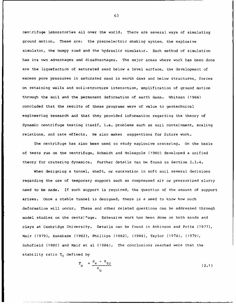
63
centrifuge laboratories all over the world. There are several ways of simulating
ground motion. These are: the piezoelectric shaking system, the explosive
simulator, the bumpy road and the hydraulic simulator. Each method of simulation
has its own advantages and disadvantages. The major areas where work has been done
are the liquefaction of saturated sand below a level surface, the development of
excess pore pressures in saturated sand in earth dams and below structures, forces
on retaining walls and soil-structure interaction, amplification of ground motion
through the soil and the permanent deformation of earth dams. Whitman (1984)
concluded that the results of these programs were of value to geotechnical
engineering research and that they provided information regarding the theory of
dynamic centrifuge testing itself, i.e. problems such as soil containment, scaling
relations, and rate effects. He also makes suggestions for future work.
The centrifuge has also been used to study explosive cratering. On the basis
of tests run on the centrifuge, Schmidt and Holsapple (1980) developed a unified
theory for cratering dynamics. Further details can be found in Section 2.3.4.
When designing a tunnel, shaft, or excavation in soft soil several decisions
regarding the use of temporary support such as compressed air or pressurized slurry
need to be made. If such support is required, the question of the amount of support
arises. Once a stable tunnel is designed, there is a need to know how much
deformation will occur. These and other related questions can be addressed through
model studies on the centr'Ouge. Extensive work has been done on both sands and
clays at Cambridge University. Details can be found in Atkinson and Potts (1977),
Mair (1979), Kusakabe (1982), Phillips (1982), (1984), Taylor (1974), (1979),
Schofield (1980) and Mair et al (1984). The conclusions reached were that the
stability ratio Tc defined by
T = v -tcc (2.1)c
u

64
where ov = total overburden pressure at the tunnel axis
atc = tunnel support pressure at collapse
Cu = undrained shear strength of the clay
for tunnels in clay lies between 3 and 9 and not necessarily at 6 as has often been
assumed. Tests on model tunnels at different scales (modeling of models) showed
good agreement. For a given clay, immediate surface deformations above the tunnel
were found to be related to the inverse of the factor of safety. There was close
agreement between predicted and observed failure mechanisms for shaft and trench
excavation. As strains increased and soil strength progressively mobilized, the
pattern of ground deformation around the tunnel or excavation remained unchanged.
Time dependent deformations were found to be due not to any viscous effect, but due
to changes in the effective stress as the excess pore pressures generated by
tunneling dissipate. In the first phase, all the pore pressures drop as the
excavation occurs. Subsequently, settlements continue as the pore pressures increase
with time. These deformations are often referred to by tunnelers as "squeeze" and it
is often wrongly concluded that the movement is due to viscous ground behavior.
Centrifuge tests coupled with effective-stress analyses using finite elements show
that the movements are uniquely related to effective stress changes in the clay. For
tunnels in clay or sand, with support conditions similar to those found in
construction, centrifuge test results were closely bracketed by the result of
theoretical studies based on upper and lower bound plasticity theorems.
The centrifue has also been used to study the slope stability of
overconsolidated clays (Fragaszy and Cheney (1981)]. The centrifuge they used
differs from conventional centrifuges in that it is a drum centrifuge, consisting of
a drum that rotates about its vertical axis. The advantage of this type of
centrifuge is that the model embankment occupies the entire circumference of the drum

65
and so forms an endless model. The tests showed that there was a combination of
prototype height and g level, beyond which only long term failure (after 1 to 8 hours
of spinning) took place.
Al-Hussaini et al (1981) modeled coal waste embankments using the centrifuge.
Various geometries were studied, and, based on the tests, it was found that estimates
of the phreatic surface based on finite element seepage analysis and Dupuit's theory
agreed with the observed results. Sutherland and Richard (1984) investigated the
development of the phreatic surface in a stable tailings dam. It was found that the
phreatic surface was only slightly affected by truncating the upstream part of the
model. Below 100g, scaling effects were minimized and the experimental results
agreed well with the theoretical results. Almeida et al (1984) studied the staged
construction of embankments on soft clay, with and without reinforcement. Their
results showed that large lateral deformations indicated low factors of safety and
that the strengthening effect of granular reinforcement columns was less important
than their effect of increasing the rate of pore pressure dissipation.
Ferguson and Ko (1984) used the centrifuge to model cone penetrometer tests.
Their results indicated that there was no unique relationship between the CPT data
and the relative density. They found that additional work was required to increase
the accuracy of predicting liquefaction potential using the cone. Moisture effects
were found to play a role in the results. Relationships among various soil
properties could be established only on a soil by soil basis. However, the results
indicated that the centrifuge could model in-situ tests.
This discussion of centrifuge research in soil mechanics is not intended to be
complete, but is provided so as to have an idea about its breadth.
2.3 Rock Mechanics
This section describes the centrifuge work that has been done in rock

66
mechanics. Most of the research was performed in the fifties and sixties, after
which the emphasis of centrifuge testing shifted to soils. Clark (1981) reviewed
research done with the centrifuge in rock mechanics, up till 1981. This review is
reported here along with more recent work. The review is broken into four sections.
The first deals with work on beams, the second with work on layered roofs,
subsidence problems, underground openings and excavations, the third with rock
slopes and rock fill dams and the fourth with miscellaneous topics.
2.3.1 Beams
Much has been done in modeling beams, since a section of a mine roof can be
represented as a beam. Bucky (1931) ran a number of centrifuge tests on simple
beams, made up of artificial material (a mixture of sand, cement and water), and of
rock (sandstone). Two series of tests were run, the first series to verify the
scaling laws and the second to show that the failure pattern obtained by self-weight
(internal) loading in the centrifuge was considerably different from the failure
pattern obtained by external pressure loading, in terms of deformations, fracture
pattern and amount of arching. As previously mentioned, this appears to have been
the first use of a centrifuge for model studies.
Caudel and Clark (1955) analyzed the stress distribution in a simple beam
subject to three different loading conditions: a) a uniformly distributed load b)
loaded by self-weight and c) loaded in a centrifuge. Two types of end conditions
were studied - a) simply supported beams and b) beams with restrained ends. The
various combinations are shown in Fig. 2.1. Their theoretical analysis showed that
the critical stresses in these simple beams could be approximated by any one of the
three types of loading, when the ratio of the length of the body to its thickness
was greater than 5. When this ratio was less than 5, then the combination of
stresses under multiple g loading caused arching rather than typical beam failure.

67
1 '-4
- -- -4
L. b -
L. 0a I. Va ~. 0.)
aa N-J -:1
S c.., - - -
1 (n
.2V
0U
'I *r4V(U0
-- V
(U
U,
0C
t - ~ ~ - 4Jt. II -4
Ii V
L. ~ K LKa aa -a 0)
aa-' 0)'p
Sn
- %rs
4., II~i. -~b 4.b (N
-4
68
They suggested that, for simple beams, the value of centrifugal testing lies not in
determining the stress distribution per se, but in finding the failure mechanism
which is different for self-weight loading as compared to external loading. Their
conclusion was that centrifuge testing would also be of use in finding the stress
distributions after failure, the post failure behavior, the stress distribution and
failure behavior of unsymmetric beams with or without rock bolts, etc.
Chan (1960) attempted to model beams using models made of gypsum rock. The
beams were 12 inches long, 2 inches wide, with thicknesses varying between I and 1.5
inches. The ends of the beam were clamped in a model holder, placed in a centrifuge
and rotated up to iailure. The behavior of the beam was observed from first fracture
to failure, using a sLroboscope. The rpm at fracture varied from 360 to 630, with
the corresponding scale factors varying from 124 to 383. Prototype beams with
dimensions equal to those of the model multiplied by the corresponding scale factor
at failure, and having the same material properties, would thus theoretically fail
due to self-weight, with the same stresses as in the model. Values of prototype beam
length at failure when plotted versus prototype beam thickness at failure, were found
to fall on a straight line in a log-log plot.
Wang et al (1967) tested simple and multiple-layer beams, simply supported or
restrained, in a 2 foot diameter centrifuge that was capable of producing up to 2700
g's. The beams were made of Bedford limestone and the bi-refringement-coating
method of photoelastic analysis used to determine the stress distributions. The
fixed beams were restrained at their ends by pouring molten type metal into end
holders and allowing it to solidify. However, this metal shrinks as it cools, and,
has a lower yield strength than rock. Consequently, the ends of the beam were
probably not rigidly fixed. This could explain why the stresses observed for these
beams were different from the theoretical values. Results for the simply supported
beams agreed well with the theory.
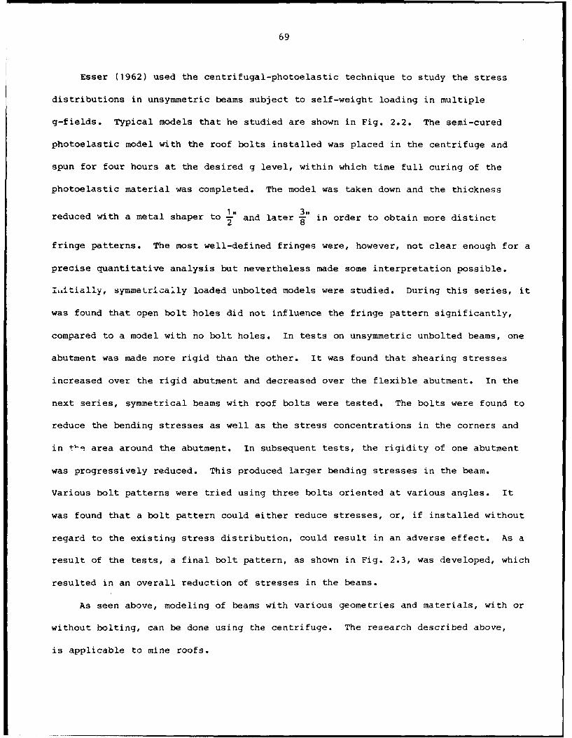
69
Esser (1962) used the centrifugal-photoelastic technique to study the stress
distributions in unsymmetric beams subject to self-weight loading in multiple
g-fields. Typical models that he studied are shown in Fig. 2.2. The semi-cured
photoelastic model with the roof bolts installed was placed in the centrifuge and
spun for four hours at the desired g level, within which time full curing of the
photoelastic material was completed. The model was taken down and the thickness
reduced with a metal shaper to - and later - in order to obtain more distinct
fringe patterns. The most well-defined fringes were, however, not clear enough for a
precise quantitative analysis but nevertheless made some interpretation possible.
iiltially, symmetrically loaded unbolted models were studied. During this series, it
was found that open bolt holes did not influence the fringe pattern significantly,
compared to a model with no bolt holes. In tests on unsymmetric unbolted beams, one
abutment was made more rigid than the other. It was found that shearing stresses
increased over the rigid abutment and decreased over the flexible abutment. In the
next series, symmetrical beams with roof bolts were tested. The bolts were found to
reduce the bending stresses as well as the stress concentrations in the corners and
in tle- area around the abutment. In subsequent tests, the rigidity of one abutment
was progressively reduced. This produced larger bending stresses in the beam.
Various bolt patterns were tried using three bolts oriented at various angles. It
was found that a bolt pattern could either reduce stresses, or, if installed without
regard to the existing stress distribution, could result in an adverse effect. As a
result of the tests, a final bolt pattern, as shown in Fig. 2.3, was developed, which
resulted in an overall reduction of stresses in the beams.
As seen above, modeling of beams with various geometries and materials, with or
without bolting, can be done using the centrifuge. The research described above,
is applicable to mine roofs.

70
44.
r 4.{-4 r ~?4A - 1. U) 0 Lo
. ~r 0 .
4.)v
41 eo
044k.4 0.
4A .4)
4J* 44
W 4-)
0%0
D4 -0
4.4)
r-4 0) 0
U U0)
~141
44 44 41)
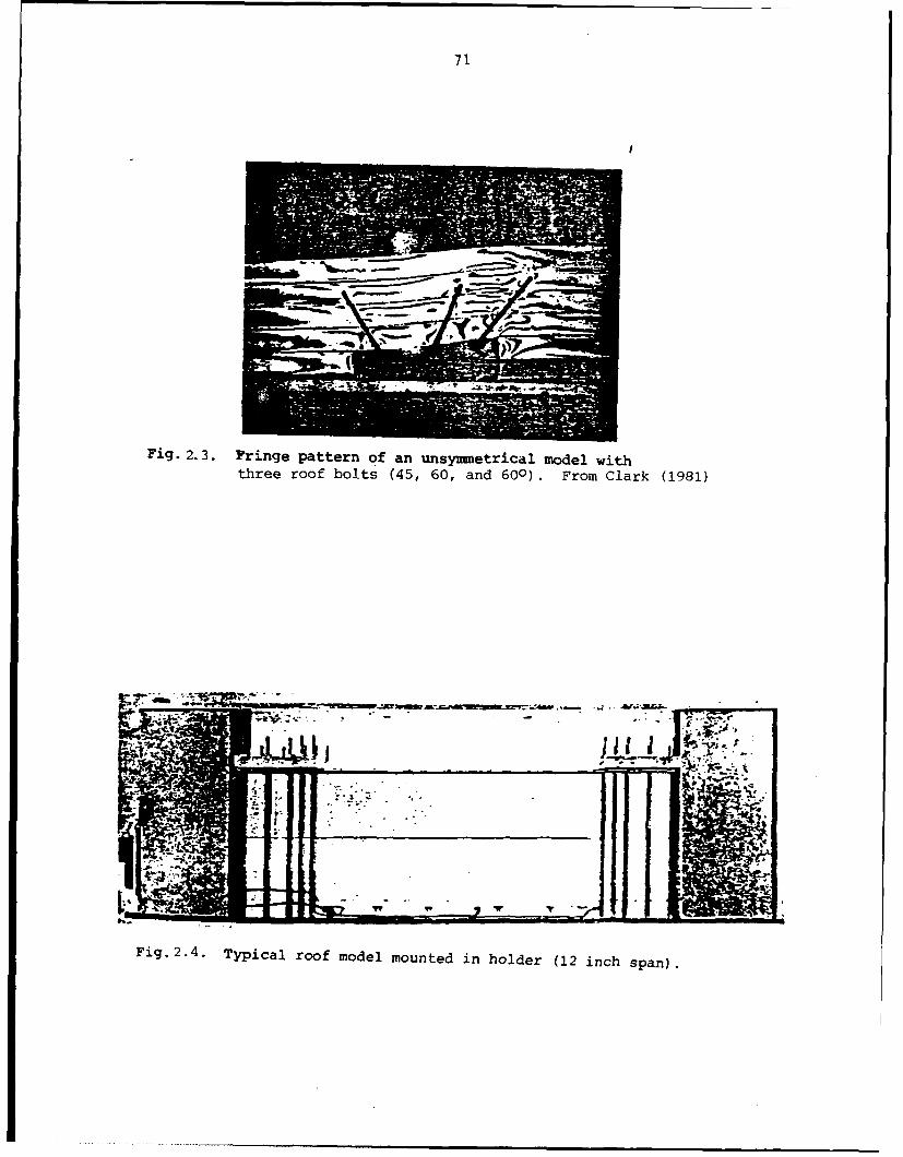
Fig. 3. Fringe pattern of an unsyimetrical model withthree roof bolts (45, 60, and 600). From Clark (1981)
Fig.2-4. Typical roof model mounted in holder (12 inch span).

72
2.3.2 Layered Mine Roofs, Subsidence Problems, Underground Openings and Excavations
Panek conducted what remains one of the most extensive investigations in rock
mechanics using the centrifuge. In this program, he designed a 6 foot diameter
centrifuge, which he enclosed in an evacuated tank (Panek (1952a, 1952b)]. He
applied dimensional analysis to the problem of bedded mine roofs reinforced by
rock bolts. The role of bolts in increasing interbed friction, in suspending the
strata and the combined effect of suspension and interbed friction were studied.
Using dimensional analysis, he was able to express the strain as a function of
seventeen H terms. It was found during the analysis that the diameter, weight,
Young's Modulus and Poisson's ratio of the bolt and the Poisson's ratio of the rock
had secondary effects and that consequently the number of TI terms could be reduced
from seventeen to six. The resulting similitude equation was
Nw L P P= o a L L hf' Pr t( 'b ' t , k , F, a, U.)
i E L r i avg
where N = centrifugal loading ratio
h = bolt length
Ei= Young's Modulus of rock of ith bed
b = bolt spacing
(ex)i = strain in ith roof bed
k = number of bolts per set across opening
t = bed thickness
wi = unit weight of rock of ith bed
Po = bolt pre-tension
Pr = least value of bolt tension that will prevent strata separation at thebolt positions
Pa = actual bolt tension
L = length of beams

73
a = coefficient from the theory of bending
F = coefficient of bedding plane friction for bolted beds
Ui = function of the relative flexural rigidity of the bolted roof beds
A series of tests were run with the variables taking values typically
encountered in practice. It was found that friction between the beddings reduces
the bending of all the beds in the unit. This interbed friction increases with the
use of tensioned bolts. If the bolts are not tensioned, then their effect is only
to suspend the less rigid layers. Hence, a pre-tensioned bolt increases the
friction between the bedded planes and also suspends the beds (layers).
Specifically, Panek (1956) investigated the frictional effect between layers of
beds, while later [Panek (1962a)] he gave details concerning the effects of
suspension. The final report of the series, Panek (1962b), documents the combined
effect of friction and suspension.
A typical model of a bolted roof is shown in Fig. 2.4. Panek's tests on the
centrifuge provided considerable insight into roof bolting and resulted in a
quantitative solution for roof bolting design. The conclusions of the study were
that the friction effect reduces the bending of all the beds in the bolted unit. As
a result of the suspension effect, the maximum outer-fibre bending stress in a bed
increases or decreases according to whether the flexural rigidity of that bed is
greater or less than the average for all the beds in the bolted unit. The net
effect of friction and suspension in a given layer was found to depend on the
bedding sequence and the bolt pre-tension. The results of Panek's research
conclusively demonstrated the usefulness of the centrifuge in solving rock structure
problems.
More recently, Stephansson (1971, 1982) conducted centrifuge tests at high g
levels (4000 g's) on layers of slabs of dimensions 20 cm x 20 cm, to study the
behavior of single openings in horizontally bedded rock. The various types of roof

74
geometries, layer stiffnesses and the types of contact between the layers (free
movement between layers vs. layers bonded together) are shown in Fig. 2.5. Once
again, the rigidity of the abutments was found to strongly influence the stresses
and deflections about the opening. The values of maximum stress in and the
deflection of a single layer roof were between those of a simply supported beam and
a fixed beam. A double layer roof, with the upper layer stiffer than the lower
layer, gave rise to separation between the layers. As the thickness of the upper
layer increased, behavior shifted towards that of a single layer roof, with
compression of the abutments under loading strongly influencing the stresses and
deformations around the openings. Results from finite element studies showed good
agreement with the centrifuge tests. For a layer with a low flexural rigidity
resting on a stiffer layer, the upper layer was found to carry part of its weight,
with the rest of its load being carried by the underlying rigid layer. Double layer
roofs made up of different materials and bonded together could be treated as
equivalent single layer T-cross-sections made up of the same material as the lower
layer.
From the result of his tests, Stephansson (1982) was able to formulate a theory
to :alculate the deflections and stresses in a mine roof area supported by pillars.
The theory was applied to the Laisvall lead mine, where detailed observations of
roof movements over a number of years are available, and good agreement between
theory and results was found.
Sutherland et al (1982) investigated subsidence over coal mines as a result of
a "longwall" operation. Such an operation is one in which a panel of coal roughly
440 yards wide by half a mile long, is removed from a coal seam, making the roof
unstable until it finally collapses. The effects of the failure migrate to the
surface, eventually creating a surface depression. Nevada Tuff, being linear up to
failure, was chosen as the model material. Each layer was 10.5 inches long, 1/8

75
IH
S INIGLE-LAYER
ROOF -L> HIncLuding S0.ear stress in
the Layer
E, 11 >E,,I1
] " Free stip along t1he cortacts
Oetnchipc
E, 1 E2 17
DOUB.LE- IVFreo s~ip along the can'.ccts
LAYER *No detaching
ROOF -- _ _ _ _ _
v WeLded contact
V1VWelded contact
MULTI -LAVER V11 Welded contactsROOF
Fig.2.5. Types of roof configurations. From Stephannson (1982).
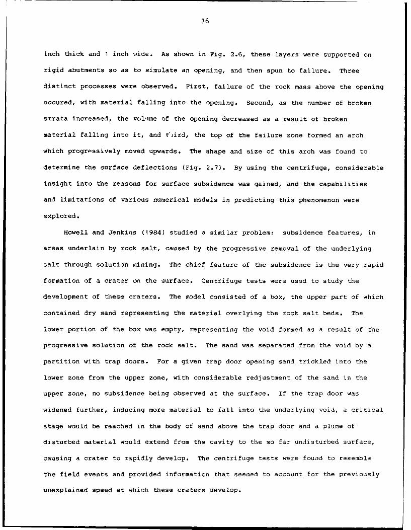
76
inch thick and 1 inch wide. As shown in Fig. 2.6, these layers were supported on
rigid abutments so as to simulate an opening, and then spun to failure. Three
distinct processes were observed. First, failure of the rock mass above the opening
occured, with material falling into the opening. Second, as the number of broken
strata increased, the voluime of the opening decreased as a result of broken
material falling into it, and t'iird, the top of the failure zone formed an arch
which progressively moved upwards. The shape and size of this arch was found to
determine the surface deflections (Fig. 2.7). By using the centrifuge, considerable
insight into the reasons for surface subsidence was gained, and the capabilities
and limitations of various numerical models in predicting this phenomenon were
explored.
Howell and Jenkins (1984) studied a similar problem: subsidence features, in
areas underlain by rock salt, caused by the progressive removal of the underlying
salt through solution mining. The chief feature of the subsidence is the very rapid
formation of a crater on the surface. Centrifuge tests were used to study the
development of these craters. The model consisted of a box, the upper part of which
contained dry sand representing the material overlying the rock salt beds. The
lower portion of the box was empty, representing the void formed as a result of the
progressive solution of the rock salt. The sand was separated from the void by a
partition with trap doors. For a given trap door opening sand trickled into the
lower zone from the upper zone, with considerable redjustment of the sand in the
upper zone, no subsidence being observed at the surface. If the trap door was
widened further, inducing more material to fall into the underlying void, a critical
stage would be reached in the body of sand above the trap door and a plume of
disturbed material would extend from the cavity to the so far undisturbed surface,
causing a crater to rapidly develop. The centrifuge tests were fouad to resemble
the field events and provided information that seemed to account for the previously
unexplained speed at which these craters develop.

77
6^. -"
Fig.2.6. Model of layered mine rocf. From Sutherland (1982).
Fig. 2.7. Fractured layers sharing the shape of the arch.From Sutherland (1982).
78
The centrifuge has been used in rock mechanics to study tunnels and other
underground openings. Oudenhoven (1962) used the centrifuge to study tunnel liners.
One of the major purposes of a tunnel liner is to support all or part of the load
of the overlying rock formation. Analytical solutions are available for stresses in
circular tunnels and shaft linings. The centrifugal technique also offers a method
of determining these stresses. Oudenhoven (1962) studied the effect of tunnel
liners on the stress distribution in the surrounding rock, by modeling them as
openings in plates made of photoelastic materials. The openings were lined with
materials of 'arious stiffnesses, placed in a centrifuge and spun. The combinations
used were
Case 1: A circular opening without a liner
Case 2: Openings in a plate of low elastic modulus, with liners of constant
thickness to radius ratio and having elastic moduli greater than the
surrounding plate, the elastic moduli of the liners being the variable.
Case 3: Openings in a plate of low elastic modulus with liners having a
constant elastic modulus higher than that of the surrounding plate, the liner
thickness being the variable.
Results for these three cases are as follows:
Case 1: The fringe pattern for the model loaded by its self-weight (the
centrifugal model) was shifted downwards as compared to the theoretical stress
distribution for loading by an externally applied uniaxial load. Also, for uniaxial
loading, there theoretically is tension at the top and bottom of the opening and the
stress concentration factor at the springline is three, whereas fcr the centrifuged
model there was no tension at the top and bottom of the opening, and the stress
concentration at the springline was 2.5. These differences were caused both by the
vertical stress gradient and by the plate holder frame which prevented the plate
model from expanding laterally, thereby inducing a snall side pressure.

79
Case 2: For these tests, it was found, as shown in Fig. 2.8, that the load was
transferred to the liner Lhrough narrow regions of high stress, the remaining plate
material surrounding the liner being relatively unstressed. The stress
concentration factors were found to increase with increase in the elastic modulus of
the liner.
Case 3: In this series, it was found that the stress concentration decreased
with an increase in liner thickness, as shown in Fig. 2.9.
More detailed studies along the above lines would result in more information
about the interaction between the liner and the rock, which could be used in the
development of better theoretical models and design methods.
Haycocks (1962) studied the stress distribution around underground openings of
various shapes, using photoelastic methods. Most of the stresses around underground
openings are due to the weight of the overlying rock, and so the centrifuge
technique is a useful way of studying them. Haycocks used semi-cured photoelastic
models into which he froze the stresses. Fig. 2.10 shows some of the openings that
were studied: (1) a circular opening; (2) a horizontal rectangular opening (see fig.
2.10a); (3) a horizontal rectangular opening with a vertical fault running down the
center and two fracture. extending from its two upper corners at an angle of about
15* from the vertical; (4) an opening with a high parabolic arch with a vertical
fault and two inclined fractures (see fig. 2.10b); and (5) a flatter parabolic arch,
with fault and fractures.
For the circular opening, the stress pattern obtained under body force loading
was similar to the stress pattern around a hole in a plate subject to external
loading at Ig except that, for the latter case, there is no stress gradient. As a
consequence of the gradient in the centrifuged model, the stress tratectories were
shifted downwards as compared to the externally loaded plate (see Fig. 2.11). As
in the case of the circular opening, the stress gradient in the centrifuged model

80
Fig.2.8. Stress pattern of rigid lining and weak plate.t/R 0.177. From Clark (1981).
4Wb
VV
a) Lining thickness of 0.452 inches, b) Lining thickness of 0.904 inches,t/R -0.354. t/R =0.708
Fig.2.9 Effect of varying~ liner -t%-!ickness. From Clark (1981).

81
tt
4 4-
A-
a) Stress pattern in rectangular openin'. b) Stress pattern in opening with %ich archwith fractures.
Fig.2.lO.Stress distribution around typical openings strjiied. From Clark (1981).
Fig.2.ll.Calibration test stress distribution.From Clark (1981).
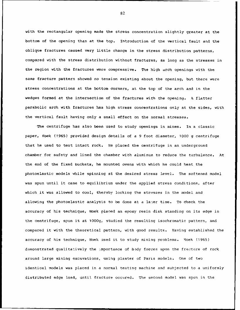
82
with the rectangular opening made the stress concentration slightly greater at the
bottom of the opening than at the top. Introduction of the vertical fault and the
oblique fractures caused very little change in the stress distribution patterns,
compared with the stress distribution without fractures, as long as the stresses in
the region with the fractures were compressive. The high drch openings with the
same fracture pattern showed no tension existing about the opening, but there were
stress concentrations at the bottom corners, at the top of the arch and in the
wedges formed at the intersection of the fractures with the opening. A flatter
parabolic arch with fractures has high stress concentrations only at the sides, with
the vertical fault having only a small effect on the normal stresses.
The centrifuge has also been used to study openings in mines. In a classic
paper, Hoek (1965) provided design details of a 9 foot diameter, 1000 g centrifuge
that he used to test intact rock. He placed the centrifuge in an underground
chamber for safety and lined the chamber with aluminum to reduce the turbulence. At
the end of the fixed buckets, he mounted ovens with which he could heat the
photoelastic models while spinning at the desired stress level. The softened model
was spun until it came to equilibrium under the applied stress conditions, after
which it was allowed to cool, thereby locking the stresses in the model and
allowing the photoelastic analysis to be done at a la:er time. To check the
accuracy of his technique, Hoek placed an epoxy resin disk standing on its edge in
the centrifuge, spun it at 1000g, studied the resulting isochromatic pattern, and
compared it with the theoretical pattern, with good results. Having established the
accuracy of his technique, Hoek used it to study mining problems. Hoek (1965)
demonstrated qualitatively the :.mportance of b.dy forces upon the fracture of rock
around large mining excavations, using plaster of Paris models. One of two
identical models was placed in a normal testing machine and subjected to a uniformly
distributed edge load, until fracture occured. The second model was spun in the

83
centrifuge until, at 600 g, failure occured. In the two cases, the resulting
fracture patterns were completely different as shown in Fig. 2.12, indicating the
influence of the body forces. Hoek (1965) also studied the stress distribution
around extensive stoping excavations on two horizons. Here, too, as shown in Fig.
2.13, stress distributions in the centrifuged model were quite different from the
case where the model was loaded externally, indicating the importance of simulating
the original stresses that exist in the rock mass. Like the previous case, the
results were only qualitative. Hoek subsequently left for Imperial College, and
thereafter not much work has been done on this machine.
Ramberg and Stephansson (1965) studied the static stability of excavations in
rock using centrifuged models. The various types of excavations they studied are
shown in column 1 of Table 2.1. The models were made up of cement, plaster of
Paris, lime, sand and magnetite powder, which were mixed in various proportions so
as to obtain the required density and strength. The models were placed in a small
centrifuge and spun to as high as 3000 g's. The results of the various tests are
shown in Table 2.1, where the column 'experimental a/g' gives the experimental ratio
between the centripetal acceleration at the moment of collapse and the acceleration
due to gravity. Similarly, the colunn 'theoretical a/g gives the calculated ratio
at failure based on the measured strength and density of the model material. The
theoretical a/g values were calculated only for models KI, K2, K3, K4, K10 and K16.
The last two cilumns give the dimensions of the equivalent prototypes made of
granite or sandstone, that would theoretically collapse due to self-weight.
2.3.3 Slope Stability
Rock slopes also too have been studied with the centrifuge. The slopes studied
were made up of photoelastic material oi homogeneous artificial rock, either intact
or with smooth joints. Rockfill dams also have been studied.

84
a) Plaster of Paris mine-model loaded to fracture by uniformly distributededge loads.
b) Plaster of Paris mine model loaded to fracture at 600 g in the centrifuge.
Fig.2.12. Fracture patterns showing the importance of body forcesin the fracture of large rock masses. From Hoek (1965).

85
a) Photoelastic pattern in a mine model subjected to uniformly distributededge loading.
b) Photoela.,tic pattern in a mine model which had been stress-frozen under acentrifugal acceleration of 100 g.
Fig. 2.l3 Comparison between photoelastic patterns under external andbody force loading. From Hoek (1965).

- 86
~0
00
a .0 fti ar
44 .0 b N .44 I I0
e~ ~ ~ 0 00 M MS V- .- - P ~ r.,gt. i'r-. -- SN 5WS 5
-c S o -0 a
Pt4451*f.
0O 0 ~ Pt
o l- U.
0 ft
-Z- vi.
ooCN ~ ~ . *.Ibe 0 v~Je~ va..@*~4S
4 1

87
Gomah (1963) studied homogeneous intact rock slopes using 2-D slope models of
photoelastic material to determine the stress distributions. The semi-cured models
were spun in the centrifuge at the desired g level until curing was complete, and
the stresses locked in the model. The model was then taken from the centrifuge and
the fringe patterns studied under polarized light. Gomah studied the stress
distributions in the slope as a function of the body stresses due to gravity, the
angle of inclination of the slope and its height. Typical stress distributions are
shown in Fig. 2.14. Loading, however, was not carried up to failure.
More recently, work has been done in Japan to study the behavior of rock
slopes. Sugawara et al (1982) studied the progressive failure of rock slopes, using
model slopes made up of a mixture of plaster, slaked lime, standard sand and water.
Three materials made up of mixtures of the above materials were used to make model
slopes, with slope angles ranging from 50 degrees to 80 degrees. A theoretical
study of the slopes, using finite elements, was also made. Fig. 2.15 is the result
of the finite element analysis and shows that if n = yH is plotted against theC
normalized strain E/Eo, then the resulting curve is useful in studying progressive
failure, where
n = a dimensionless factor indicating the magnitude of gravitational loading
y = unit weight of the material
H = height of slope
c = cohesion of the material
= strain measured on the rock surface
Eo = material constant which is the elastic axial strain at the
uniaxial compressive strength
At n = ni, failure initiates at the toe of the slope. At n = nt, the strain increment
on the surface of the slope changes from compression to tension, and at n = nc, the
strain increment becomes infinite which is the condition of limiting equilibrium.
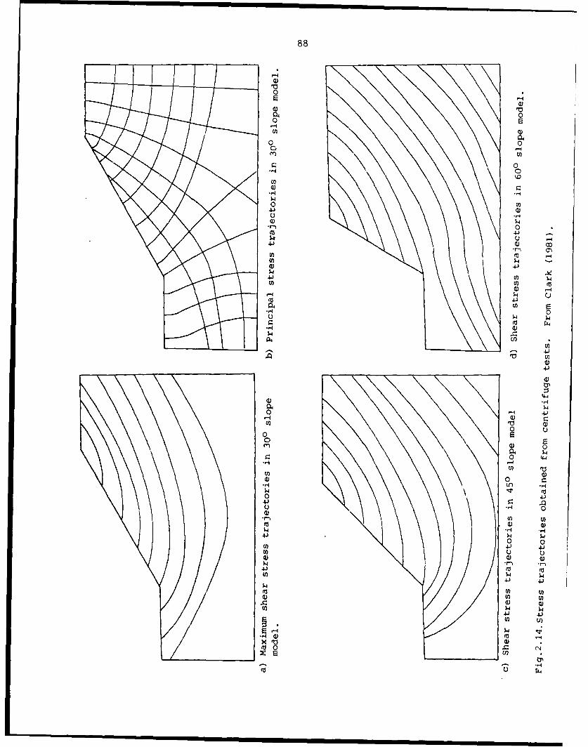
88
0
000 E
04 0
U)
00
4)-
U)U
4
o) En
04 U)0
04 UU)4-
U) U)
0
04 )00
0
.- -4 U
U)24) 0
0
4-0 --4
0- 0U) u
$44
mU)
0D 0f
41 4
U) U
-4
rd a) 4-)
4

89
20 20ACr 0=30"
.- nI
I CJ 0 [ (b)'o 01 02 Q3 0.4 9080706050
V/l. i (degre)a) Relation between n b) Relations between n, n , n. and i
and 6/ o0
Fig. 2.15. Results obtained by FEM analyses. From Sugawaraet al (1982).
a) Reaton bewe nd'5 ti=udges
SOT%%: A *C
I mj:B
eC S 14 0. 9. 3.0 310f90 2
ata
02 01, 02 0110 OSC/6.
a) Relations between ni and cIE0 at i = v degrees.
0:8 A Mo.del -y E CP OP cr or ElepI A 140 80.5 137.0 30.0 34.0 29.0 588
IS 3 B 142 60.8 97.9 30.0 31.0 29.0 621Calculated . C 145 40.3 71.3 30.0 34.0 29.0 565
Calculated ' I .
10 to 20, e) Model geometry and physical/ EI
/ /properties of materials.
5 10
O:A Ack bFDA0:8
00 0So~S 70 60 0 5070SoSi(geer i (degree) i (dree)
b) Relations c) Relations d) Relationsbetween between betweenn and i. n and i. n' and i.
C C
Fig.2.16.lResults of centrifuge tests on intact rock slopes. From L:ugawara et al (1982).

90
Sugawara et al suggested that the change from compression to tension of the strain
increment measured on the surface was the result of progressive sliding on the slip
lines, and that consequently n = nt represented a stable-unstable transition.
Progressive failure should be clearly detected at n > nt .
The results from the centrifuge tests are shown in Fig. 2.16 and are similar to
the finite element results. Also shown in Fig. 2.16 are the properties of the model
materials, the model geometry and the relation between nt, nc and n' (n' = -H_ wherecc cres
cres is the cohesion intercept of the residual strength) and the slope angle i.
Sugawara et _-1 showed that nt was a linear function of i (Fig. 2.16). The value of n
at which limiting equilibrium was reached was n = nc . Based on their work, they
suggested that using the peak shear strength of the rock mass to calculate the
limiting slope height was unrealistic as strain softening is thereby ignored. On the
other hand, using the residual shear strengths would be too conservative.
Consequently they suggested that the analysis be based on the plot of nt (the
transition from stable to unstable conditions) vs. i.
Sugawara et al also analyzed a slope with a discontinuity. Fig. 2.17
shows the model geometry, material propertiltz and results of the centrifuge tests,
1plotted as curves of n vs. , for 0 = i and ' = j. The terms 1, H, a, i and j
are defined in Fig. 2.18. The theoretical analysis with which the expelimental
results were compared is also shown in this figure. The model assumes the
simultaneous sliding of the failure wedge on both the potential slip plane GB in the
intact rock and the joint surface DG. This assumption is valid only at the very
start of sliding, or if the rock wedge is perfectly rigid, as otherwise movement on
the two planes will not take place at the same time. In the experimental model
(the material not being perfectly rigid), differences were observed between the test
results and the results of the theoretical analyses. This is shown in Fig. 2.17

91
0"s ittnuTL_ of7Sm 160*
0-
-4 0.2 00 04 0.6 0.8 -02 0 0.2C/C. C/C.
a) Relations between n and e/eo at O< /H<0.24.
15, i - I 15
Sample: O Sample: E
10 C1 ) r I tntact2 rock rateal Joint surface
C Model CP vp C" or r" 6"
D 138.0 30.0 30.0 29Q 5.0 22.0
IE 62.0 30.0 33.0 29.0 10.0 24.0
c) Model geometry and physical
properties of materials.
L/H I2H
b) Relatiol between nc , nt and I/H.
Fig. 2.17. Results of centrifuge tests on jointed rock slopes. From Sucawaraet al (1982).
.,/C i D ct~a-c}
/ ;" sin.,.NccS.4Sin =W,
TC.CS-!,NcsI s6 P =0.P? WS Ini ,- - c ----,s
cosV-i-o')
-----------
>7 -. ----......... (3)
R H -------,Ic.V - (4.)
k,---.h tan(,"v' -*P2),=SJ-&-dsmfl s~n/ ,
Fig.2.18. A failure model of slope with a discontinuity.From Sugawara et al (1982).

92
where the dotted line is a plot of the theoretical value of n (calculated using
Equation 4 in Fig. 2.18), plotted vs 1/H. From the experimental results, it is seen
that the theoretical analysis does not define the limiting equilibrium condition but
corresponds to the stable-unstable transition. This is because the simultaneous
sliding on the two planes as assumed in the theoretical analysis, is, for an
imperfectly rigid material, valid only up till the stable-unstable transition. This
test series showed clearly how theoretical modeling and centrifuge testing go hand
in hand.
Mikasa et al (1982) ran stability tests on a rock fill dam using a centrifuge.
The dam in question was a zoned dam with an inclined core and was to be built on
unfavorable deposits, with its downstream zone made up of weak weathered material.
They did not expect accurate results from finite element analyses and so decided to
model the problem with the centrifuge. Eleven types of 2-D dam models were tested,
of which the results of tests run on three models (models 7, 9 and 10) were
presented. Details of these three models are shown in Fig. 2.19. For modeling the
rock material, sandstone was pulverized to a maximum diameter of 4.8 mm, which was
1/150 the size of the prototype material. To model the core and the downstream
material, particles of the core material from the site, under 2mm in size, were
used. The model dimensions were made 1/150 those of the prototype and the model was
centrifuged at 150 g. The tests were done in three stages. In the first stage, the
g level was raised to 150 g over a period of 5 minutes. In the second stage, the
upstream water level was raised from the base to 0.9 times the dam height, and then
lowered back to the base. This cycle was repeated five and a half times so that, at
the start of the third stage, the water level was near the dam crest. For the third
stage, the model was inclined to the upstream side by 0.02 radians over a period of
6 seconds, and held in this position for 4 seconds, after which, it was brought to
the vertical position again. The procedure was repeated until failure occured, and
was to simulate lateral earthquake action statically.
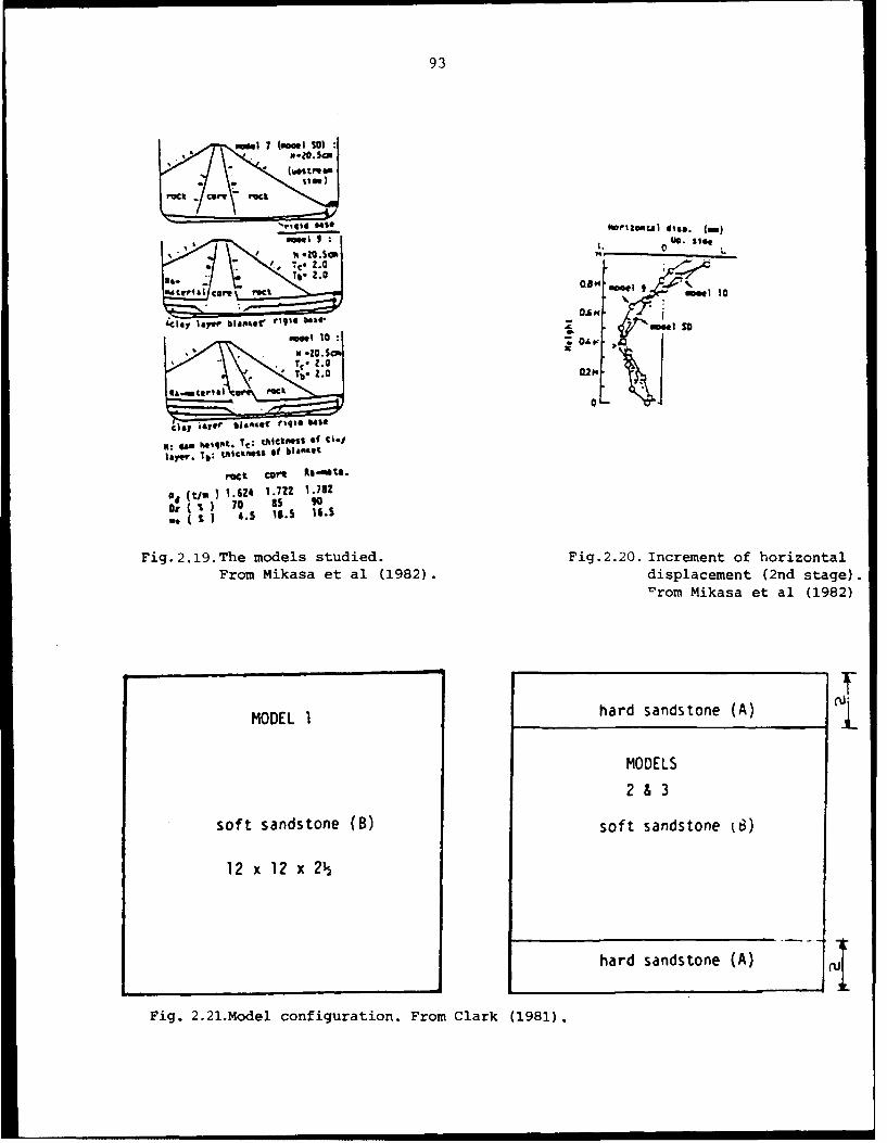
93
M .' ti 7 (mot S0) :I ,+ \ "% .20.5o S
Pu+-lqld k** "DrIZ RL&II igst1 . (M)
"c tp' lfie'Il S a . 0 £
owet 1 : 1 Up sleet
N -tO.SmT. Z.0
N:W lt. To:e U~ne( s ofu ease
tU I: 45 P~aqt tC tIICWf l C .Ie
rock Iort Ral.09?A.
*8 (j/ ) 1.624 1.722 1.732Mw" 70 85 CA
,,Q~ ~ ~~ ( ; .S1.S .Sm
Fig.2.19.The models studied. Fig.2.20. Increment of horizontal
From Mikasa et al (1982). displacement (2nd stage).rom Mikasa et al (1982)
MODEL hard sandstone (A)
MODELS
2&3
soft sandstone (B) soft sandstone t8)
12 x 12 x 2
hard sandstone (A) nil
Fig. 2.21.Model configuration. From Clark (1981).
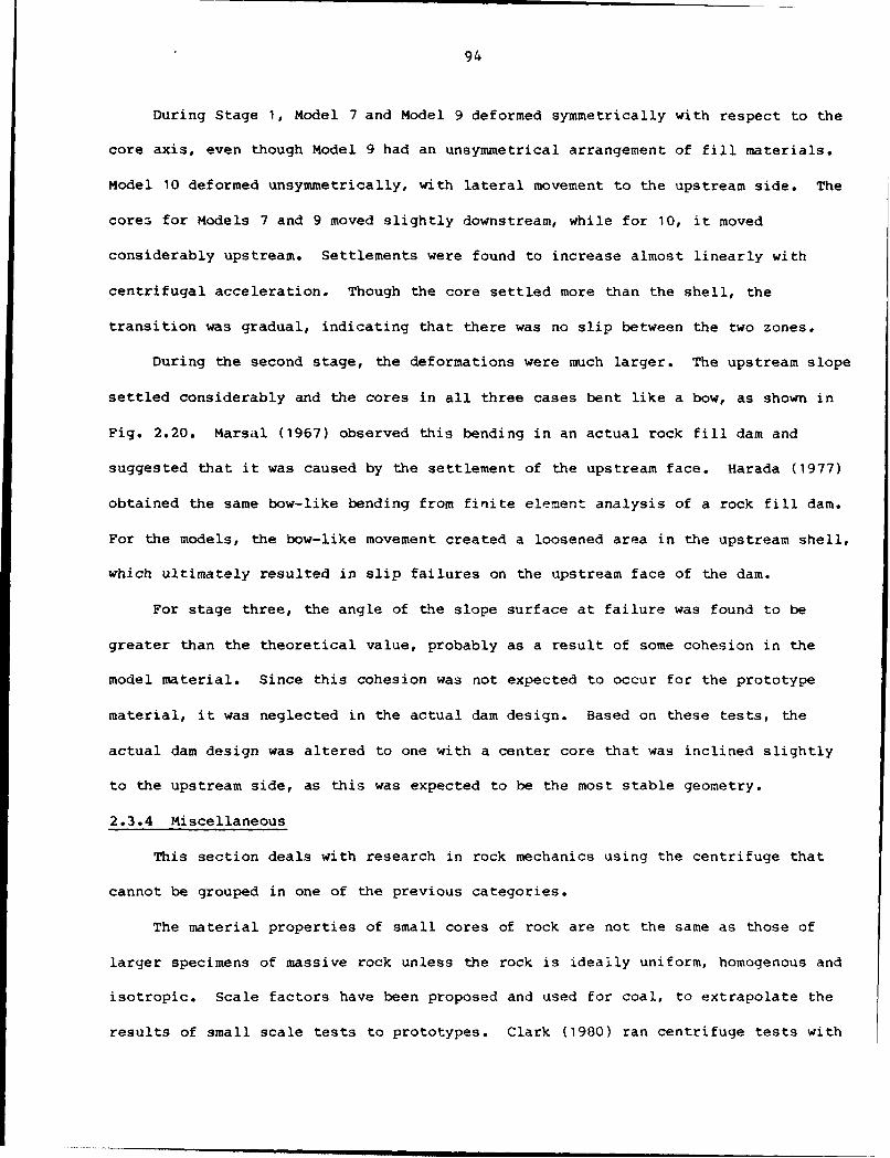
94
During Stage 1, Model 7 and Model 9 deformed symmetrically with respect to the
core axis, even though Model 9 had an unsymmetrical arrangement of fill materials.
Model 10 deformed unsymmetrically, with lateral movement to the upstream side. The
cores for Models 7 and 9 moved slightly downstream, while for 10, it moved
considerably upstream. Settlements were found to increase almost linearly with
centrifugal acceleration. Though the core settled more than the shell, the
transition was gradual, indicating that there was no slip between the two zones.
During the second stage, the deformations were much larger. The upstream slope
settled considerably and the cores in all three cases bent like a bow, as shown in
Fig. 2.20. Marsal (1967) observed this bending in an actual rock fill dam and
suggested that it was caused by the settlement of the upstream face. Harada (1977)
obtained the same bow-like bending from finite element analysis of a rock fill dam.
For the models, the bow-like movement created a loosened area in the upstream shell,
which ultimately resulted in slip failures on the upstream face of the dam.
For stage three, the angle of the slope surface at failure was found to be
greater than the theoretical value, probably as a result of some cohesion in the
model material. Since this cohesion was not expected to occur for the prototype
material, it was neglected in the actual dam design. Based on these tests, the
actual dam design was altered to one with a center core that was inclined slightly
to the upstream side, as this was expected to be the most stable geometry.
2.3.4 Miscellaneous
This section deals with research in rock mechanics using the centrifuge that
cannot be grouped in one of the previous categories.
The material properties of small cores of rock are not the same as those of
larger specimens of massive rock unless the rock is ideally uniform, homogenous and
isotropic. Scale factors have been proposed and used for coal, to extrapolate the
results of small scale tests to prototypes. Clark (1980) ran centrifuge tests with

95
flat sandstone slabs cut with the large faces normal to the bedding planes. The
slab dimensions were 12 inches x 12 inches x 2 1/2 inches. In order that stresses
be evenly distributed, the slabs were surface ground on all the outside surfaces.
As most rocks in large mases are not uniform in properties or composition, no
attempt was made to select a slab of exceptional uniformity.
Two sandstcnes - sandst,A A and sandstone B - were used to make three models of
a large intact rock slab. Sandstone A had a higher modulus of elasticity than
sandstone B. Fig. 2.21 shows the models that were tested. Model 1 was made entirely
of sandstone B, while Models 2 and 3 had layers of sandstone A of different
thicknesses at the top and bottom. The layered models were placed in the centrifuge
bucket and spun to check whether any effects due to bedding would become evident
during testing, and whether these effects scaled with the g level. Strain gages were
mounted at various points on the surface of the sandstone. The gages showed a wide
range of readings with some gages even indicating that yield had occured, i.e. the
stress-strain properties of the rock appeared to vary with position. This shows
that it would be desirable to consider the properties of a rock as a function of
position, for input into theoretical .,oa-Is.
Clark (1981) has suggested that the centrifuge can play an important role in
studying explosive cratering in rock. Schmidt and Holsapple (1980) modeled
cratering in sand using small amounts of explosive in a multiple gravity field.
They developed a unified theory for cratering dynamics in terms of source
characteristics, energy and specific energy, soil strength, gravity, time and the
range over which debris were distributed. The equations were applied to the case of
an explosive detonated on the surface of a deformable soil medium with the space
above the medium being filled with gas. Schmidt et al identified eight
independent variables that they thought controlled cratering phenomena, and, by
using dimensional analysis, obtained five w terms, one of which showed that the

96
Em 3yield of an exposion scaled at N3 i.e. E - N , where Em is the energy yield of the
model explosion and Ep is the yield of the prototype explosion. There has been some
discussion as to whether the energy yield scales at the third power or fourth power
of N, or at some value in between. Using the Boeing centrifuge, they were able to
successfully simulate explosions in a range of soil types, with the values of the
dimensionless terms chosen so as to cover the equivalent of twelve orders of
magnitude of explosive energy. Schmidt and Holsapple (1980) suggested that by
modifying the variables to account for the properties of rock, it would be possible
to run the same types of tests to study cratering phenomena in rock. The relative
cost of experimental prototype scale cratering is several orders of magnitude
greater than that of an equivalent small scale test as the centrifuge, clearly
showing the cost effectiveness of the centrifuge in studying prototype behavior.
Early centrifuge work dealt with problems involving rock. Most of the
centrifuge work in the fifties and sixties too dealt with rock. In the latter half
of the sixties, more interest was shown in studying soil problems in the centrifuge,
until, in the seventies, very little work if any, was done on rock problems. In the
eighties, there has been a renewed interest in studying problems dealing with rock.
From the previous sections, it is clear that centrifuge testing is a technique
that can be used to advantage in rock mechanics to study a wide range of problems.
Most of the work described previously deals only with intact rock material, with
little or no work done with jointed rocks or rock masses. The centrifuge technique
could possibly be of considerable use in investigating this area. A second report
will explore these possibilities.
2.4 Ice Mechanics
Oil exploration is being carried out from off-shore structures in Arctic areas.
For the efficient design of structures in these areas, an idea about the ice forces

97
exerted by the surrounding ice fields on these structures is required. Vinson (1982)
proposed the use of a centrifuge to study these forces. Of interest were the
magnitudes of the forces exerted on the structure, the failure mechanisms and
details on factors influencing general ice behavior. The variables of interest
suggested were the ice temperature, thickness and salinity, the flow velocity and
the angle of incidence of impact with the structure.
Clough et al (1986) describe the development of a program to test ice behaviQ
in the centrifuge. Four components were involved: I) the insulated strong box to
contain the model, 2) a system for forming the ice sheet, 3) a drive system to pull a
structure through the ica sheet (effects similar to a sheet moving past the
structure) and 4) the instrumentation. The various components are shown in Fig. 2.22.
The model strong box was build of aluminum, lined on the insides with 1/4 inch
acrylic plastic and on the outside by 1 inch thick polystyrene foam. By doing this,
the heat flow was made essentially unidirectional, with the heat flow through the
sides and the base only 1% of the flow through the ice covered surface. To form the
ice sheet, liquid nitrogen was injected through holes along a circular boundary ring
(Fig. 2.22). The nitrogen vapor was held in the container by an acrylic plastic
cover held in place by a wing nut. Using this system it was possible to create a
fairly uniform ice sheet. A motor placed on the centrifuge platform, with its shaft
passing through the container wall and connected to a worm drive through a flexible
coupling (Fig. 2.23), was used to pull a 1 inch diameter aluminum rod, mounted on a
base plate, through the ice sheet. Feedback loops were used to maintain
temperatures at desired levels and also to control the velocity of movement of the
structure. Temperatures were monitered at different spots using thermistors.
Movement of the structure was measured with LVDT's. Loads on the structure were
measured by strain gauges attached to the bottom of the aluminum rod. The entire
system was found to work well and data from centrifuge tests compared well with the
results of in-situ tests reported in the literature.

98
Aluminurn ThermnistorsStrong Boz
To Liquid Nitrogen
ModelPileInsulatlion
Driv MotorStrain Gages La ce
LVOT
Fig. 2 .22 .Sectional view of model test container. From Clough et al (1986) .
eso. 0
weauia Model Structure
ice Load Screw Assembly
1.0 alAluminum Rod S ockgo"e Plate
Strmn Gave$
Unislide se
Fig. 2.2-aModel structure assembly. From Clough et al (1986).

99
Clough and Vinson (1985) studied the ice forces on vertical structures using the
apparatus described above. From a dimensional analysis they obtained five
dimensionless products which they used to conduct the centrifuge model tests. Based
on their results, they concluded that small scale tests, if properly interpreted, can
describe large scale forces for the crushing mode of failure. They found that
centrifuge modeling of ice-structure interaction is valid, and provides a way of
scaling self-weight forces of the ice, for gravity dependent problems. For the
crushing mode of failure in thin ice sheets, a small scale model will accurately
describe the prototype if the model dimensions are at least thirteen times the
average ice crystal size. The normalized force on the structure for the crushing
mode of failure is constant for a ductile type failure, in accordance with plasticity
theory, but for some reason rises to a peak in the transition from ductile to brittle
failure. The normalized force on a frictionless conical structure for the bending
mode of failure is proportional to the tangent of the cone angle, linearly dependent
on the normalized inertial acceleration (centrifugal acceleration) and independent of
the normalized velocity for normalized velocity values less than or equal to I x
10- 3. Measured horizontal forces agree well with theoretical predictions. Lastly,
they concluded that the small scale modeling technique was valid for the crushing
model of ice-structure interaction investigated and that the results of their study
could be used to predict ice forces due to ice crushing on rigid isolated vertical
structures in either fresh or saline ice.
Professor Schofield at Cambridge University, England, has modeled ice on the
centrifuge. Lovell and Schofield (1986) detail the procedure used to form the ice
sheets. Sixty-five litres of water with a salinity of 3% is cooled by liquid
nitrogen. The nitrogen boils steadily for 4 1/2 hours due to heat entering the
nitrogen. The cold gas falls to the surface of the water, extracts the heat and
rises to leave the package. It was found that the time to develop an ice sheet of
100
25 mm at 60 g was just over an hour. The time required at i g to form a sheet of
equivalent thickness (60 x 25 = 1500 mm) is about 6 months. It was found that the
grain size of the salt ice scales to the correct order of magnitude. Also,
appropriate scaling of the random, transition and columnar zones as in the first year
sea-ice was obtained. It was also found that the rate of increase of horizontal
crystal diameter with depth of the ice was in good agreement with that of first year
sea-ice. The ice sheets were tested under vertical static loads, by layering dead
weights onto the ice at the center of the sheet. Comparison of the breakthrough
loads with recommended loadings showed the results to be of the same order as those
expected. Further studies involving lateral loads, various scales and loading rates
were proposed. A drum centrifuge capable of 500 g is to be built, with which bigger
ice sheets can be modeled.
2.5 Tectonics
The centriruge has also been used in experimental tectonics. Ramberg (1963)
started a project modeling tectonic processes at the University of Chicago. He then
went to Uppsala, Sweden where the method was further developed to the point where it
was considered a routine method of testing. The centrifuge at UrFsal.A that Ramberq
used could accelerate a mass of 1.5 kg to 3000 g.
Tectonic processes are difficult to model at 1g. The prototype structures are
so large (ranging from hundreds of meters to hundreds ot kilometers) that gravity
effects play a role in their evolution. In a scaled model the self weight stresses
at Ig are very small. Also, due to the high strength and viscosity of the material,
prototype structures deform very slowly. Consequently, in order that deformations
develop reasonably quickly under the low stresses that exist at I g, the model
material should be made far weaker than the prototype material. True similarity at
ig requires model material that is so weak that it is often impossible to construct
models from these materials. In his pioneering work in modeling tectonic processes,

101
Ramberg (1963) overcame this problem by subjecting his models to an elevated gravity
field, using the centrifuge. By increasing self-weight stresses, he was able to
satisfy similitude requirements using stiffer and more viscous model materials.
Commonly used model materials included: 1) silicone putty of various viscosities,
either pure, or mixed with fine powder of magnetite or tungspar (or both) to obtain
the desired density, 2) painters putty with a plastic base, 3) mixtures of
collophony and ethylene phthalate, 4) modeling clay or Dlasticene, 5) oil-wax
mixtures and 6) K Mn 04 solutions.
Various prototype tectonic processes which are driven and controlled by gravity
have been successfully modeled in the centrifuge. Ramberg (1968 a, 1968b, 1972)
studied the formation of mantled domes (Fig. 2.24), extrusion of lava, folding of
layered complexes, subsiding bodies, and other processes powered by gravitational
instability. He was also able to model continental drift.
Dixon and Summers (1982) used a centrifuge capable of reaching 20,000g, at the
Experimental Tectonics Laboratory at Queens University in Ontario, Canada, to model
tectonic processes. The centrifuge consists of a 33 inch diameter disc of solid
aluminum, 3.25 inches thick, and provided with two diametrically opposed cavities to
hold the samples. The general types of problems they studied were the convective
overturn of unstable density stratification, and the gravitational collapse and
lateral spreading of a rock mass elevated with respect to the gravitational
equipotential surface. Specific problems that were examined were the progressive
evolution of mantled Gneiss Domes [Dixon (1975)], the incernal geometry, strain
distribution and progressive deformation of simple Greenstone Belts (Dixon and
Summers (1980), (1981)] and folding and faulting in layered materials [Dixon and
Summers (1982)]. Wuantitative data concerning the strain distribution within the
structure were obtained by contructing the model in two halves, with passive
internal layering. The layering is horizontal in one half and vertical in the other

102
B -..-.
'A . , 74-, _,,
4cm
".-+ .",9 -D ,% .C+i, -N +"+i
Fig. 2 .24 .(A) Dome of silicone putty (0 = 1.4 g/cm3) having penetratedoverburden of painters putty (0 1.87 g/cm 3) during centrifugation.
Initial structure consisted of horizontal parallel and continuous layers.H = hat of dome, T =trunk. Arrows indicate rim syncline. (B) Silicone-putty dome (light gray, with thin, dark sheet that has broken intoboudins) rises through painter's putty overburden. Substratum (black)consists of heavy silicone putty mixed with powder of magnetite. Notebulge on substratum below dome. Original layering horizontal. (C) Layerof light silicone putty that has risen through overburden of ;ainter'sputty, spread across the surface, and sucked up the heavy substratumalmost to the surface. (D) Model indicating direction of flow insource layer and dome. The initially evenly thick horizontal sourcelayer consisted of alternating strips of dark and light colored siliconewith square cross section as indicated by two vertical lines on leftside of photo. Present pattern indicates movement. Note that horizontalflow in source layer has passed un-derneath the rim syncline. FromRamberg (1972).

103
as shown in Fig. 2.25, so that, when two layers in the undeformed model - on-j from
each half - are superimposed, a square grid is obtained. After deformation, two
corresponding sections, similarly superimposed, will yield a deformed grid. By
comparing the deformed grid with the undeformed grid, the orientation and magnitude
of maximumi deformation in each grid eletuent can be obtained, as shown in Fig. 2.26.
A grid of l4 -ies can also be drawn on the surface of the model to study surface
deformations. The advantage of this method is that information regarding large
deformations, which would cause a break down of numerical schemes, can be obtained.
Also, this method provides a detailed three-dimensional picture of the evolution of
the structure.
Large scale tectonic processes are complex in terms of configuration,
rheological properties, boundary stresses, displacement conditions, significant
local heterogenities in the displacement field, and finite strains. Consequently,
they are difficult to model correctly using current numerical methods. Physical
modelling using the centrifuge offers an additional tool, for obtaining information
about these processes.
2.6 Conclusion
This section briefly summarizes the work done in geotechnical engineering using
the centrifuge and also suggests areas in rock mechanics where the technique will
be of use.
At present, the most frequent application of the centrifuge in geotechnical
engineering is in soil mechanics. Centrifuges in various countries are being used
to study a wide range of problems involving soil. The work being done can be
considered as falling under one of the following headings - the flow of water through
soils, soil-structure interaction, dynamics, underground construction and other uses
such as slope stability, embankments, penetrometer studies, etc.

104
L..ZQ:
Fig.-2.25. Three stages in the development of a Mantled Gneiss Dome.TOP row: two sections through model WD-4. Note that in one sectionthe striped pattern in the buoyant layer and in the imediateoverburden was initially vertical, anJ in the other section, horizontal.If the two striped patterns are superimposed, the deformed aridof Fig.2.26is produced. Middle and bottom rows: two more advancedstages of growth of the-dome (models WD-2 and WD-3). (Models describedin detail in Dixon, 1975). From Dixon and Summers (1982).

105
JillIh, -
-.--.-- - --------- --- - t
- -- , , .\ -
Fig.2.26.Deformfed grid elements of Mantled Gneiss Dome model WD-4
(Dixon, 1975), showing the orientation and relative magnitude of
the axis of maximum finite elongation in each grid element.
From Dixon and Summers (1982).
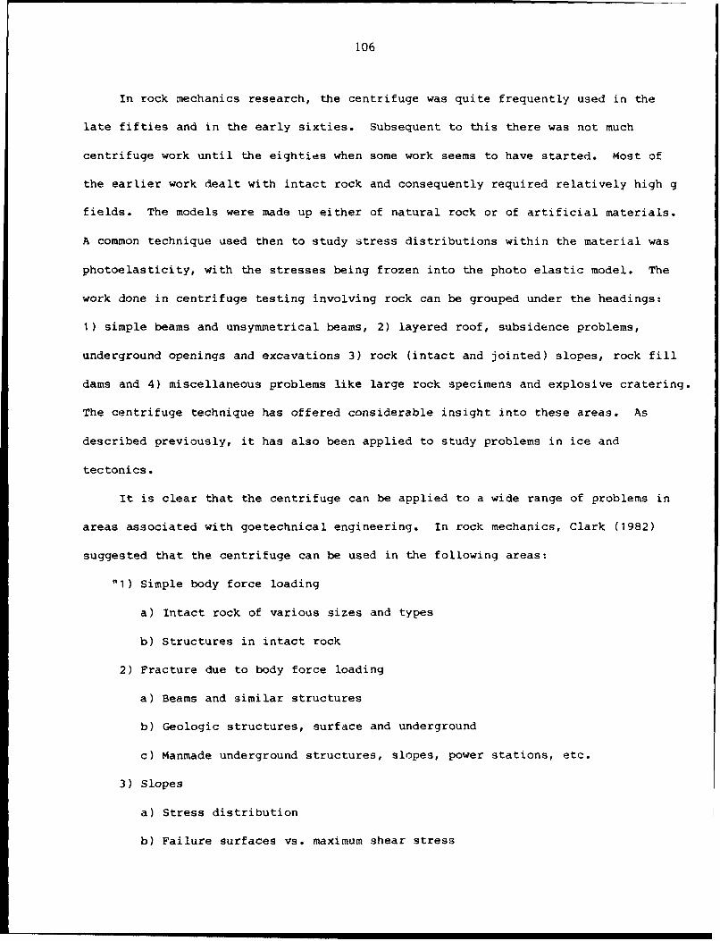
106
In rock mechanics research, the centrifuge was quite frequently used in the
late fifties and in the early sixties. Subsequent to this there was not much
centrifuge work until the eighties when some work seems to have started. Most of
the earlier work dealt with intact rock and consequently required relatively high g
fields. The models were made up either of natural rock or of artificial materials.
A common technique used then to study stress distributions within the material was
photoelasticity, with the stresses being frozen into the photo elastic model. The
work done in centrifuge testing involving rock can be grouped under the headings:
1) simple beams and unsymmetrical beams, 2) layered roof, subsidence problems,
underground openings and excavations 3) rock (intact and jointed) slopes, rock fill
dams and 4) miscellaneous problems like large rock specimens and explosive cratering.
The centrifuge technique has offered considerable insight into these areas. As
described previously, it has also been applied to study problems in ice and
tectonics.
It is clear that the centrifuge can be applied to a wide range of problems in
areas associated with goetechnical engineering. In rock mechanics, Clark (1982)
suggested that the centrifuge can be used in the following areas:
"1) Simple body force loading
a) Intact rock of various sizes and types
b) Structures in intact rock
2) Fracture due to body force loading
a) Beams and similar structures
b) Geologic structures, surface and underground
c) Manmade underground structures, slopes, power stations, etc.
3) Slopes
a) Stress distribution
b) Failure surfaces vs. maximum shear stress

107
c) Rock slides
d) Fractured solid rock slopes, stress and stability
4) Behavior of rock masses with and without similitude (qualitative studies)
5) Mechanics of caving, with and without similitude (qualitative studies)
6) Many other types of investigations where body forces are dominant."
Most, if not all of the research described previously deals with intact rock.
Problems involving sliding along the discontinuities have not been modeled with the
centrifuge. The reason is that the shear behavior of a joint may be governed by the
magnitudes of absolute displacement. If this is the case, then scaling may result
in a loss of similitude as regards displacement related behavior. A future report
will deal in detail with the scaling relations for both intact rock and jointed
rock. Also included in that report will be suggestions for future research in rock
mechanics (including problems in jointed rock masses), using the centrifuge.

108
References
Al-Hussaini, M.M., Goodings, D.J., Schofield, A.N. and Townsend, F.C. (1981),
"Centrifuge Modeling of Coal Waste Embankments," ASCE, Journal of the
Geotechnical Engineering Division, Vol. 107, No. GT 4, April.
Almeida, M.S.S. and Parry, R.H.G., (1984), "Penetrometer Apparatus for Use in
the Centrifuge During Flight," Proceedings of the Application of CentrifugeModelling to Geotechnical Design, Editor W. H. Craig, University Gf
Manchester.
Almeida, M.S.S., Davies, M.C.R. and Parry, R.H.G. (1985), "Centrifuge Tests of
Embankments on Strengthened and Unstrengthened Clay Foundations,"
Geotechnique, Vol. 35, No. 4, pp. 425-441.
Andersen, G.A., (1987), "Tilting Response of a Centrifuge Model Gravity
Retaining Wall to Seismic Shaking," Masters Thesis, M.I.T., Cambridge,Massachusetts.
Anandrajah, A., Arulanandan, K. and Hutchinson, J.R. (1985), "Difficulties inthe Simulation of Dynamic Events in a Centrifuge," Second Symposium on the
Interaction of Non-Nuclear Munitions with Structures, Panama City, Florida.
Arulanandan, K., Anandarajah, A., Abghari, A. (1982), "Centrifugal Modellingof Soil Liquefaction Susceptibility," ASCE, Journal of Geotechnical
Engineering, Vol. 109, No.3, March.
Barton, Y.O. (1984), "Response of File Groups to Lateral Loading in the
Centrifuge," Proceedings of the Application of Centrifuge Modelling toGeotechnical Design, Editor W. H. Craig, University of Manchester.
Bloomquist, D.G., Davisdon, J.L., and Townsend, F.C. (1984), "PlatformOrientation and Start-up Time During Centrifuge Testing," Geotechnical Testing
Journal, GTJOOJ, Vol. 7, No. 4, Dec. 1984, pp. 195-199.
Bolton, M.D. (1984), "The Development of Aulti-Anchor Eartt -ententionSystems," Proceedings of the Application of Centrifugal Modelling to
Geotechnical Design, Editor W. H. Craig, University of Manchester.
Bolton, M.D. and Steedman, R.S. (1982), "Centrifuge ModelLing of the
Response of Microconcrete Retaining Walls subjected to Shaking." Proc. Conf.Soil Dynamics and Earthquake Eng., Southhampton, 13-15 July, pp. 311-329.
Bolton, M.D. and Steedman. R.S. (1984), "The Behavior of Fixed CantileverWalls Subject to Lateral Shaking," Proceedings of the Application of
Centrifuge Modelling to Geotechnical Design, Editor W. H. Craig, University of
Manchester.
Bucky, P.B. (1931), "Use of Models for the Study of Mining Problems,"American Institution of Mining and Metallurgical Engineers, Tech. Pub. 425,
3-28.
Cargill, K.W. and Ko, H.Y. (1984), "Centrifugal Modelling of Transient WaterFlow," ASCE, Journal of Geotechnical Engineering, Vol. 109, No.4.

109
Caudel, R.D. and Clark, G.B. (1955), "Stresses Around Mine Openings in Somesimple Geologic Structures," University of Illinois Engineering ExperimentalStandard Bulletin 430.
Chan, S.M.C. (1960), "Physical Properties Tests of Rock, Centrifugal Tests andthe Design of Mine Openings," M.S. Thesis, University of Missouri School ofMines.
Cheney, J. (1982), "Introduction to Geotechnical Centrifuge Modelling,"Proceedings of a Workshop on High Gravity Simulation for Research in RockMechanics, Colorado School of Mines, Department of Mining Engineering, Golden,Colorado.
Clark, G.B. (1980), "Investigation of Effects of Sample Size onCompressibility Coefficients," Report for Sandia Laboratories, New Mexico.
Clark, G.B. (1981), "Geotechnical Centrifuges for Model Studies and PhysicalProperty Testing of Rock and Rock Structures," Colorado School of MinesQuarterly, Vol. 76, No. 4.
Clough, H.F., Vinson, T.S. (1985), "Ice Forces on Vertical CylindericalStructures," Draft of Paper.
Clough, H.F., Wurst, P.L., Vinson, T.S. (1986), "Determination of Ice Forceswith Centrifuge Models," Geotechnical Testing Journal, GTJODJ, Vol. 9, No. 2,1986, pp. 49-60.
Craig, W.H. and Al-Saoudi, N.K.S. (1981), "The Behaviour of Some ModelOff-shore Structures", Tenth ICSMFE, Vol. 1, pp. 83-88, Stockholm.
Craig, W.H. (1984), "Installation Studies for Model Piles," Proceedings of theApplication of Centrifuge Modelling to Geotechnical Design, Editor W.H. Craig,University of Manchester.
Croce, P., Pane, V., Znidarcic, D., Ko,H.Y., Olsen, H.W. and Schiffman, R.L.,(1984), "Evaluation of Consolidation Theories by Centrifuge Modelling,"Proceedings of the Application of Centrifuge Modelling to Geotechnical Design,Editor, W.H. Craig, University of Manchester.
Davidenkov, N.N. (1936), "A New Method of Using Models for the Study ofEquilibrium of Structures," Technical Physics of the USSR, Vol. III, No. 1,1936, pp. 131-136.
Davis, M.C.R., and Parry, R.H.G. (1983), "Shear Strength of Clay in CentrifugeModels," ASCE, Journal of Geotechnical Engineering, Vol. 109, No. 10, October.
Dixon, J.M. (1975), "Finite Strain and Progressive Deformation in Models ofDiapiric Structures," Tectonophysics, Nol. 26, pp. 89-124.
Dixon, J.M. and Summers, J.M. (1980), "A Centrifuged Model Study of theTechtonic Development of Archean Greenstone Belts," Geoscience Research GrantProgram Summary of Research, 1979-80, Ontario Geological Survey, MP 93, pp.58-71.

110
Dixon, J.M., and Summers, J.M. (1981), "A Centrifuged Model Study of the
Tectonic Development of Archean Greenstone Belts," Geoscience Research GrantProgram Summary of Research, 1980-81, Ontario Geological Survey MP 98, pp.54-66.
Dixon, J.M. and Summers, J.M. (1982), "High-G Centrifuge Modelling ofGeological Structures," Proceedings of a Workshop on High Gravity Simulationfor Research in Rock Mechanics, Colorado School of Mines, Department of MiningEngineering, Golden, Colorado.
Esser, R.H.K, (1962), "A Model Study of the Application of Roof Bolts UnderUnsymmetrical Loading Conditions," M.S. Thesis, University of Missouri School
of Mines.
Ferguson, K.A., and Ko, H.Y. (1984), "Application of Centrifugal Modelling toCone Penetrometer Technology," Proceedings of the Application of CentrifugeModelling to Geotechnical Design, Editor, W.H. Craig, University ofManchester.
Fragaszy, R.J. and Cheney, J.A. (1981), "Drum centrifuge Studies ofOverconsolidated Slopes", ASCE, Journal of the Geotechnical EngineeringDivision, Vol. 107, No. GT7, July.
Finn, W.D.L., Barton, Y.O., Tolohata, 1. (1984), "Dynamic Lateral Response ofPile Foundations: Centrifuge Data and Analysis, " Proceedings of theApplication of Centrifugal Modelling to Geotechnical Design, Editor, W.H.Craig, University of Manchester.
Gemperline, M.C. and Ko, H.Y. (1984), "Centrifugal Model Tests for UltimateBearing Capacity of Footings on Steep Slopes in Cohesionless Soils,"Proceedings of the Application of Centrifugal Modelling, to GeotechnicalDesign, Editor, W.H. Craig, University of Manchester.
George, P.J. and Shaw, P.G.H. (1976), "Certification of Concrete GravityPlatforms in the North Sea", Offshore Technology Conference Paper OTC 2436.
Goodings, D.J. (1979), "Centrifugal Modelling of Slope Failures," Ph.D.Thesis, Cambridge University.
Goodings, D.J. (1984), "Relationships for Modelling Water Effects inGeotechnical Models," Proceedings of the Application of Centrifuge Modellingto Geotechnical Design, Editor, W.H. Craig, University of Manchester.
Gomah, A.H. (1963), "An Application of Photoelasticity to the Stability ofSlopes," M.S. Thesis, University of Missouri School of Mines.
Halliday, D. and Resnick, R. (1981), "Fundamentals of Physics," John Wiley andSons, Inc. pp. 816.
Harada, T. (1977), "A Study on Stability Analysis, Design and Construction ofRockfill Dams," Doctoral Thesis, Osaka City University.

111
Haycocks, C. (1962), "Mechanics of a Voussoir Arch," M.S. Thesis, Universityof Missouri School of Mines.
Hoek, E. (1965), "The Design of a Centrifuge for the Simulation ofGravitational Force Fields in Mine Models," Journal of South African Instituteof Mining and Metalurgy, Vol. 65, No. 9.
Kimura, T., Kusakabe, 0., Saitoh, K. (1984), "Undrained Deformation of Clay ofwhich Strength Increases Linearly with Depth," Proceedings of the Applicationof Centrifugal Modelling to Geotechnical Design, Editor:, W.H. Craig,University of Manchester.
Kimura, T., Kusakabe, U., Saitoh, K. (1985), "Geotechnical Model Tests ofBearing Capacity Problems in a Centrifuge," Geotechnique, Vol. 35, No. 1, pp.33-45.
Ko, H.Y., (1982), "Centrifuges and Soil Mechanics', Proceedings of a Workshopon High Gravity Simulation for Research in Rock Mechanics, Colorado School ofMines, Dept. of Mining Engineering, Golden, Colorado.
Kusakabe, 0. (1982), "Stability of Excavations in Soft Clay," Ph.D. Thesis,University of Cambridge.
Kutter, B.L. (1982), "Centrifugal Modelling of the Response of ClayEmbankments to Earthquakes," Ph.D. Thesis, Cambridge University.
Langhaar, H.L. (1951), "Dimensional Analysis and Theory of Models," John Wileyand Sons, New York.
Laut, P. (1975), "Application of Centrifugal Model Tests in Connection withStudies of Flow Patterns of Contaminated Water in Soil Structures,"Geotechnique, Vol. 25, pp. 401-406.
Lyndon, A., Pearson, R. (1984), "Pressure Distribution on a Rigid RetainingWall in Cohesionless Material," Proceedings of the Application of CentrifugalModelling to Geotechnical Design, Editor, W.R. Craig, University ofManchester.
Mair, R.J. (1979), "Centrifugal Modelling of Tunnel Construction in SoftClay," Ph.D. Thesis, University of Cambridge.
Mair, R.J., Phillips, R., Schofield, A.AN. and Taylor, R.N. (1984),"Apolication of Centrifuge Modelling to the Design of Tunnels and Excavationin -oft Clays," Proceedings of the Application of Centrifugal Modelling toGeotechnical Design, Editor: W.H. Craig, University of Manchester
Malushitsky, Y.N. (1981), "The Centrifugal Model Testings of Waste HeapEmbankments," English translation of Russian, 1975 edition, CambridgeUniversity Press.
Marsal, R.J., Arellano, L.R. (1967), "Performance of El Infiernillo Dam,"ASCE, SM4, pp. 265-297.
. ... 1
m m m m m mmmm m m m m wTi,1l

112
Mikasa, M., Mochizuki, A. and Matumoto, T. (1982), "Stability Test of aRockfill Dam by Centrifuge," International Conference on Soil Mechanics andFoundation Engineering, pp. 475-478.
Nakase, A., Kusakabe, 0., Wong, S.F. (1984), "Centrifuge Model Tests onBearing Capacity of Clay," ASCE, Journal of Geotechnical Engineering, Vol.110, No. 12, pp. 1749-1765.
Nunez, I.L. and Randolph, M.F. (1984), "Tension Pile Behavior in Clay -Centrifuge Modelling Techniques," Proceedings of the Application ofCentrifugal Modelling to Geotechnical Design, Editor: W.H. Craig, Universityof Manchester.
Oldham, D.C.E. (1984), "Experiments with Lateral Loading on Single Piles inSand," Proceedings of the Application of Centrifugal Modelling to GeotechnicalDesign, Editor: W. H. Craig, University of Manchester.
Oudenhoven, M.S. (1962), "A Model Study of the Behavior of Elastic Liners inZAallw Undarground Openings," M.S. Thesis, University of Missouri, School ofMines.
Ovesen, N.K. (1975), "Centrifugal Testing Applied to Bearing Capacity Problemsof Footings on Sand", Geotechnique, Vol. 25, No. 2, 394-401.
Padfield, C.J. and Schofield, A.N. (1983), "The Development of centrifugalModels to Study the Influence of Uplift Pressures on the Stability of a FloodBank," Geotechnique, Vol. 33, No. 1, pp. 57-66.
Panek, L.A. (1949), "Design of Safe and Economical Structures," Transactionsof the American Institute of Mining and Metallurgical Engineers, Vol. 181, pp.371-375.
Panek, L.A. (1952a), "Centrifugal-Testing Apparatus for Mine-StructureAnalysis," U.S. Bureau of Mines Report of Investigations 4883.
Panek, L.A. (1952b), "Centrifugal-Testing Apparatus for Mine-Structure StressAnalysis," U.S. Bureau of Mines Report of Investigations 4884.
Panek, L.A. (1956a), "Theory of Model Testing as Applied to Roof Bolting,"U.S. Bureau of Mines Report of Investigations 5154.
Panek, L.A. (1956b), "Design of Bolting Systems to Reinforce Bedded MineRoof," U.S. Bureau of Mines Report of Investigations 5155.
Panek, L.A. (1956c), "Principles of Reinforcing Bedded Mine Roof with Bolts,"U.S. Bureau of Mines Report of Investigations 5156.
Panek, L.A. (1962a), "The Effect of Suspension in Bolting Bedded Mine Roof,"U.S. Bureau of Mines Repor* of Tnvestigations 6138.
Panek, L.A. (1962b), "The Combined Effects of Friction and Suspension inBolting Bedded Mine Roof," U.S. Bureau of Mines Report of Investigations 6139.

113
Panek, L.A. (1982), Proceedings of a Workshop on High Gravity Simulation forResearch in Rock Mechanics, Colorado School of Mines, Dept. of MiningEngineering, Golden, Colorado.
Phillips R. (1869), "Computes Reudus de l'Academie des Sciences," Paris,Jan-June, p. 68.
Phillips, R., (1982), "Trench Excavations in Clay," M. Phil. Thesis,University of Cambridge.Phillips, R. (1984), "Forthcoming Ph.D. thesis," University of Cambridge.
Pokrovsky, G.I. (1933), "Zeitschrift for Technische Physics," Vol. 14, No. 4.
Pokrovsky, G.I. and Fyodorov, I.S. (1936), "Studies of Soil Pressures andDeformations by Means of a Centrifuge," Proceedings, 1st. Int. Conf. on SoilMech., Vol. 1., No. 70.
Prevost, J.H. Cuny, B. and Scott, R.F. (1981), "Offshore Gravity Structures:Centrifugal Modeling," ASCE, Journal of the Geotechnical Engineering Division,Vol. 107, No. GT2.
Ramberg, H. (1968a), "Instability of Layered Systems in the Field of Gravity,I." Phys. Earth Planet Int., V.1, pp. 427-447.
Ramberg, H. (1968b), "Instability of Layered Systems in the Field of Gravity,II." Phys. Earth Planet, Int., V. 1, p. 448-474.
Ramberg, H. (1972), "Inverted Density Stratification and Diapirism in theEarth: Journal of Geophysical Reseatch, Vol. 77, p. 877-9e9.
Rowe, P.W. (1975), "Displacement and Failure Models of Model Offshore GravityPlatforms funded on Clay", Conf. Offshore Europe 75, pp. 218, 1-17, SpearheadPublications, Aberdeen.
Rowe, P.W. and Craig, W.H. (1976), "Studies of Offshore Caissons founded onOosterschelde Sand", Conf. on Design and Construction of Offshore Structures,pp. 49-55, Inst. of Civil Engineers, London.
Rowe, P.W. and Craig, W.H. (1978), "Predictions of Caisson and PierPerformance by Dynamically Loaded Centrifugal Models", Symp. on FoundationAspects of Coastal Structures, Paper IV.3, pp. 1-16.
Rowe, P.W. and Craig, W.H. (1980), "Applicatiun of Models to the Prediction ofOffshore Gravity Platform Foundation Performance", Int. Conf. on Offshore SiteInvestigation, pp. 269-281, Graham and Trotman, London.
Sabagh, S.K. (1984), "Cyclic Axial Load Tests on Piles in Sand," Proceedingsof the Application of Centrifugal Modelling in Geotechnical Design, Editor:W.H. Craig, University of Manchester.
Schmidt, R.M. and Holsapple, K.A. (1980), "Theory and Experiments on CentrifugeCratering," J. Geophysics. Res. 85(B1), 235-252.

114
Scott, R.F. (1979a), "Cyclic Lateral Loading of Piles, Analysis of CentrifugeTests," Research Program for API-OASAPR, Project 13. Calif. Inst. Tech.
Scott, R.F. (1979b), "Cyclic Static Model Pile Tests in a Centrifuge," Proc.11th Offshore Technology Conference, pp. 1159-1168, Paper OTC 3492.
Scott, R.F. (1981), "Pile Testing in a Centrifuge," Proc. 10th Int. Conf. onS.M.F.E., Stockhold, Vol. 2, pp. 839-842.
Stephansson, 0. (1971), "Stability of SIngle Openings in Horizontally BeddedRock," Engineering Geology, Vol. 5, pp. 5-71.
Stephansson, 0. (1982), "Stability of Single Openings in Horizontally BeddedRock," Proceedings of a Workshop on High Gravity Simulation of Research inRock Mechanics, Colorado School of Mines, Department of Mining Engineering,Golden, Colorado.
Sutherland, H.J. (1982), "Centrifuge Simulations of the Subsidence Over CoalMines and the Stability of Tailings Dams," Proceedings of a Workshop on HighGravity Simulation for Research in Rock Mechanics, Colorado School of Mines,Department of Minings Engineering, Golden, Colorado.
Sutherland, H.J. and Rechard, R.P. (1984), "Centrifuge Simulations of StableTailing Dam," ASCE, Journal of Geotechnical Engineering, Vol. 110, No. 3,March.Tan, T.F. and Scott, R.F. (1985), "Centrifuge Scaling Considerations forFluid-Particle Systems," Geotechnique, Vol. 35, No. 4, pp. 461-470.
Taylor, R.N. (1979), "Stand-up of a Model Tunnel in Silt," M. Phil. Thesis,University of Cambridge.
Taylor, R.N. (1984), "Grand Movements associated with Tunnels and Trenches,"Ph.D. Thesis, University of Cambridge.
Trott, J.J., Taylor, R.N. and Symons, I.F. (1984), "Tests to ValidateCentrifuge Modelling of Flexible Pipes," Proceedings of the Application ofCentrifugal Modelling to Geotechnical Design, Editor: W.H. Craig, Universityof Manchester.
Vinson, T. S. (1982), "Ice Forces on Offshore Structures," Proceedings of aWorkshop on High Gravity Simulation for Research in Rock Mechanics, ColoradoSchool of Mines, Department of Mining Engineering, Golden, Colorado.
Wang, C.S., Boshkov, S.H. and Wane, M.T. (1967), "The Application ofBarodynamic Photostress Techniques to the Study of the Behavior of Rock BeamsLoaded by Their Own Weight," 9th Symp. -n Rock Mech., Am. Inst. ofMetallurgical Engineers.
Whitman, R.V. (1984), "Experiments with Earthquake Ground Motion Simulation,"Proceedings of a Symposium on the Application of Centrifuge Modelling toGeotechnical Design, Editor: W. H. Craig, University of Manchester.


![Centrifuge Modelling With Transparent Soil and Laser Aided ...eprints.whiterose.ac.uk/125617/1/38_2015_[J14]_Centrifuge modellin… · within the field of geotechnical engineering](https://static.fdocuments.in/doc/165x107/6048e07a88fbe118e1066863/centrifuge-modelling-with-transparent-soil-and-laser-aided-j14centrifuge-modellin.jpg)