A Numerical Scheme for the Denoising ofElectrocardiogram Signals

S. Cuomo, G. De Pietro, R. Farina, A. Galletti and G. Sannino

RT-ICAR-NA-2015-2 Marzo 2015

This paper has been accepted for publication as a full paper in Elsevier Procedia CS

and oral presentation at the International Conference on Computational Science

(ICCS) 2015 - Reykjavık, Iceland (1-3 June, 2015).

1

A Numerical Scheme for the Denoising ofElectrocardiogram Signals

S. Cuomo1 , G. De Pietro2, R. Farina2, A. Galletti3 and G. Sannino2

RT-ICAR-NA-2015-2 Marzo 2015

This paper has been accepted for publication as a full paper in Elsevier Procedia CS

and oral presentation at the International Conference on Computational Science

(ICCS) 2015 - Reykjavık, Iceland (1-3 June, 2015).

1 University of Naples Federico II, Department of Mathematics and Applications, Naples,

Italy.

2 Institute for High-Performance Computing and Networking, National Research Council

(ICAR-CNR), Naples, Italy.

3 University of Naples Parthenope, Department of Science and Technology, Naples, Italy

I rapporti tecnici dell’ICAR-CNR sono pubblicati dall’Istituto di Calcolo e Reti ad

Alte Prestazioni del Consiglio Nazionale delle Ricerche. Tali rapporti, approntati

sotto l’esclusiva responsabilita scientifica degli autori, descrivono attivita di ricerca

2

del personale e dei collaboratori dell’ICAR, in alcuni casi in un formato preliminare

prima della pubblicazione definitiva in altra sede.

1 Sommario

L’ elettrocardiogramma (ECG) e una registrazione dell’attivita elettrica deimuscoli del cuore, generalmente utilizzato per l’analisi delle malattie car-diache. Gli impulsi elettrici del cuore possono essere misurati attraversodegli elettrodi, indossabili, durante le attivita fisiche o giornaliere. Tut-tavia, la qualita di questi segnali acquisiti viene sempre degradata dallapresenza del rumore, durante la fase di acquisizione. In questo lavoro, pro-poniamo uno schema numerico per il denoising dell’ ECG, con un costo com-putazionale di tipo lineare. La bassa complessita computazionale e dovutoal fatto che il metodo proposto appartiene alla classe dei filtri con rispostaimpulsiva infinita (IIR). Il principale contributo dello schema proposto e cheesso non richiede una diretta applicazione della Fast Fourier Trasform (FFT)per l’eliminazionde delle frequenze del rumore. Inoltre, lo schema proposto,offre la possibilita di una semplice implementazione utile soprattutto peril filtraggio su dispositivi di elaborazione mobile. Esperimenti che testanol’accuratezza e la complessita computazionale sono presentati per testarel’algoritmo.

3

Abstract

High quality Electrocardiogram (ECG) data is very important becausethis signal is generally used for the analysis of heart diseases. Wearablesensors are widely adopted for physical activity monitoring and for theprovision of healthcare services, but noise always degrades the qualityof these signals. In this paper, we propose a novel numerical scheme forECG Signal denoising with low computational requirements. It is com-putationally cheap because it belongs to the class of Infinite ImpulseResponse (IIR) noise reduction algorithms. The main contribution ofthe proposed scheme is that it does not require a direct application ofthe Fast Fourier Transform. Moreover, it offers the possibility of imple-mentation on mobile computing devices in an easy way. Experimentson real datasets have been carried out in order to test the algorithm.

2 Introduction

The accurate analysis of noisy Electrocardiogram (ECG) data is a very in-teresting challenge. This is especially true in relation to the pervasive useof wearable healthcare monitoring systems [1], where physiological data ac-quired from real life can be used for remote healthcare scenarios, for the earlyanalysis of diseases, as in e.g. [2], or for the highlighting of correlations be-tween health and a correct lifestyle, as in e.g. [3]. The ECG biomedicalsignal is composed of weak non-stationary data which are affected by vari-ous types of noises: power line interference, baseline drift, electromyographyinterference and sensor contact noise. Generally, a good denoising schemehas the capability of removing noises, from the acquired signal, by filteringthe data and by ensuring a result as close as possible to the unknown origi-nal signal. In literature, there are numerous research papers devoted to thisproblem, including: adaptive filtering [4, 5], Wiener filtering [6], EmpiricalMode Decomposition [7], and wavelet denoising [8] (for other methods see[9]). In ECG filtering, a crucial problem is the preservation of the sharp,that is achieved by several algorithms, for example by non local means filter-ing [10]. Unfortunately, these schemes are quite computationally expensive.In this paper, starting from a methodology based on Recursive Filtering,applied successfully by the authors in another research field [11, 12, 13], wepropose a novel numerical scheme for ECG Signal denoising with low com-putational costs, in terms of memory and time. Our approach is based onthe analysis of the signal in the Fourier domain, but it does not require adirect application of the (Fast) Fourier Transform. With respect to othermethods, we compute the solution with only a few floating point operations.This feature makes the scheme suitable for direct implementation in appli-cations on mobile devices, dedicated to the real time filtering of biomedicalsignals. In order to test the algorithm, we report the performance met-rics achieved by applying the proposed methodology to some records of the

4

database PhysioNet [14], that offers a large collection of recorded physiolog-ical ECG signals. The paper is organized as follows: in section 2 we givesome preliminary mathematical considerations; section 3 is devoted to thenumerical scheme; in section 4 we report the numerical experiments and,finally, in section 5 we draw our conclusions.

3 Mathematical Preliminaries

In this section we present a scheme for the filtering of digital signals with acomputational cost of O(n) floating point operations. This scheme is basedon an approximation of a continuos convolution with a suitable homogeneousand isotropic correlation function h (e.g. [15]) . Let s0 denote a real functionsuch that

s0 = s+ ε

with s the original signal and ε a noise function. In computer vision, re-searchers as in (e.g. [16]) use the convolution of s0 with a function h,Lebesgue integrable, to obtain a denoised function sh by s0, i.e.

sh(t) = [h ∗ s0](t) =

∫ +∞

−∞h(t− x)s0(x)dx, ∀t ∈ R. (1)

The focus of this section is to determine suitable properties for the functionh in order to determine a denoising scheme. The scheme has to eliminatenoises ε s.t. the frequency spectrum is wandering in a limited range. Toachieve this aim we use the following mathematical tools:

• the Fourier Transform F of a signal f

F (ω) = F(f)(ω) =1√2π

∫ +∞

−∞f(x)e−iωxdx, ∀ω ∈ R; (2)

• the Fourier anti-Transform F−1 of F

f(t) = F−1(F )(t) =1√2π

∫ +∞

−∞F (x)eitxdx, ∀t ∈ R; (3)

• the convolution theorem

F(h ∗ f) = F(h) · F(F ) = H · F ; (4)

The main idea of this work is to find a suitable convolution kernel h, todenoise s0, starting from its Fourier Transform H = F(h) in the Fourierdomain. Now, let us suppose that

Sh = F(sh), S0 = F(s0), S = F(s) and E = F(ε).

If we assume that the Fourier Transform H = F(h) of h is such that:{H · S = S,

H · E = 0,(5)

5

then, it can be easily proved that it holds that:

sh = h ∗ s0 ≡ s. (6)

Observing that, if the original and noise signals, s and ε, have the property

suppS ∩ supp E = ∅, (7)

then, it is possible to obtain an infinite class of functions that satisfy condi-tion (5). Then, in these hypotheses, the original signal s can be completelyrestored by the convolution in (6). Nevertheless, as shown in the next exam-ple, a satisfying solution sh (an approximation of s) can be achieved withoutassuming (7), and by filtering the signal s0 by means of a certain convolutionkernel.

Figure 1: Top: an ECG signal s. Bottom: F−Transform S = F(s) of s

Figure 2: Top: the noisy ECG signal s0 = s+ ε. Bottom: F−Transform S0 = F(s0) ofs0 , sum of S = F(s) (black line) and of E = F(ε) (red line)

Now, let s be an original ECG signal (top of Figure 1) and s0 = s+ ε (top ofFigure 2) the noisy signal, obtained by the noise function ε. Here we take ε asthe Base Line Wander noise (e.g.[7]) Assuming that the interval [µ−σ, µ+σ]contains the support of the Fourier Transform E , i.e. supp E ⊆ [µ−σ, µ+σ],

6

then we consider a convolution kernel h = F−1(H), where H is set as

H(ω) =

{0 if ω ∈ [µ− σ, µ+ σ]

1 otherwise(8)

With these assumptions, a way of obtaining a denoised signal sh is given bythe following steps:

(i) F-Transform s0, to obtain S0 = F(s0) = S+ E (S and S0 are shown, respec-tively, in the bottom of Figures 1 and 2);

(ii) define the function H as in (8);

(iii) multiply H for S0, to achieve Sh = H · S0 (top of Figure 3);

(iv) F−1-Transform Sh = H · S0, to extract from s0 the signal sh = F−1(Sh)(bottom of Figure 3).

All these figures have been generated by a Matlab code (Code 1) thatuses the Fast Fourier Transform (FFT) and Inverse Fast Fourier Transform(IFFT) (e.g. Van Loan), in order to implement steps (i)–(iv). This codetakes into account the symmetry of supp E in the Fourier domain, when ε isa periodic function. In particular in Code 1, the parameters µ, σ of (8) areset as µ = 0, 4 Hz and σ = 0, 3 Hz.

Figure 3: Top: the restored signal sh. Bottom: F−Transform Sh = F(sh)

func t i on s h = FFT Filter ( s 0 ,mu, sigma ) ;% Inputs : % s 0 vec to r no i sed input dataf l =(mu−sigma )/ f s %normal ized lower f requency and ;fu=(mu+sigma )/ f s %normal ized upper f requency to cut ;S 0 = f f t ( s 0 , n , 2 ) ;H=ones (1 , n ) ;k =f l o o r ( f l ∗n ) : f l o o r ( fu ∗n)H(1 , k ) = 0 ; H(1 , n−k+2) = 0 ;S h (1 , : )=H( 1 , : ) . ∗ S 0 ( 1 , : ) ;s h= r e a l ( i f f t ( S h , n , 2 ) ) ;

Code 1: Matlab Code of a FFT Filter for Base Line Wander in ECG signals

7

We highlight that the bottom of Figure 2 indicates that suppS∩supp E 6= ∅,but after applying the Code 1, in which H is set as 0 also on suppS∩supp E ,the signal sh can anyway be considered an accurate approximation of s.However, the mathematical form of H in (8), and its discontinuities, preventus from determining our numerical scheme. Therefore, for our purpose, aswe will show in the next section, instead of H, we will use a function H thatemulates the properties of H. This function is defined as

H(ω) =(ω − µ)2

2σ2 + (ω − µ)2, ∀ω ∈ R. (9)

and is a rational approximation of the function

G(ω) = 1− e(−(ω−µ)2/2σ2), ∀ω ∈ R. (10)

Notice that H is obtained from G, by taking the first two terms in the Taylorexpansion of the following exponential function

e((ω−µ)2/2σ2) =

+∞∑i=0

1

i!

((ω − µ)2

2σ2

)i(11)

The functions H(ω) and G(ω) share the following properties:

1. 0 ≤ G(ω), H(ω) < 1, ∀ω ∈ R ;

2. H(µ) = G(µ) = 0;

3. limω→±∞

H(ω) = limω→±∞

G(ω) = 1;

4. H(ω) and G(ω) are symmetrical with respect to the axis ω = µ ;

5. H(µ± σ) = 1/3;

6. H(ω) = Hl(ω) · Hr(ω), ∀ω ∈ R, where we set

Hl(ω) =−iω + iµ

−iω + (√

2σ + iµ), Hr(ω) =

iω − iµiω + (

√2σ − iµ)

. (12)

It is still possible to compute the denoised signal sh by means of Code 1,

replacing H in (9) instead of H in (8).The choice of function H in (9) can determine the noisy ε, even if its fre-quency spectrum is wandering in the interval [µ− σ, µ+ σ]. Moreover, withthis function, it is possible to provide a numerical scheme to obtain thedenoised function sh from s0 as shown in next section.

4 A novel O(n) Numerical Scheme

In this section, we introduce the derivation of our scheme for the denoisingof digital signals. This algorithm is based on the Infinite Impulse Response(IIR) Gaussian Recursive Filter of [17] and [18]. It reduces the effects ofadditive noise functions ε on the original signal s, when supp E ⊂ [µ−σ, µ+σ]. In terms of floating point operations, this algorithm is faster than FFT.

8

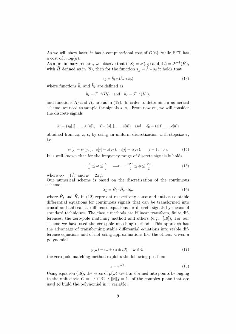
As we will show later, it has a computational cost of O(n), while FFT hasa cost of n log(n).As a preliminary remark, we observe that if S0 = F(s0) and if h = F−1(H),with H defined as in (9), then for the function sh = h ∗ s0 it holds that

sh = hl ∗ (hr ∗ s0) (13)

where functions hl and hr are defined as

hl = F−1(Hl) and hr = F−1(Hr),

and functions Hl and Hr are as in (12). In order to determine a numericalscheme, we need to sample the signals s, s0. From now on, we will considerthe discrete signals

~s0 = (s0[1], . . . , s0[n]), ~s = (s[1], . . . , s[n]) and ~ε0 = (ε[1], . . . , ε[n])

obtained from s0, s, ε, by using an uniform discretization with stepsize τ ,i.e.

s0[j] = s0(jτ), s[j] = s(jτ), ε[j] = ε(jτ), j = 1, ..., n. (14)

It is well known that for the frequency range of discrete signals it holds

−πτ≤ ω ≤ π

τ⇐⇒ −φd

2≤ φ ≤ φd

2(15)

where φd = 1/τ and ω = 2πφ.Our numerical scheme is based on the discretization of the continuousscheme,

Sh = Hl · Hr · S0. (16)

where Hl and Hr in (12) represent respectively cause and anti-cause stabledifferential equations for continuous signals that can be transformed intocausal and anti-causal difference equations for discrete signals by means ofstandard techniques. The classic methods are bilinear transform, finite dif-ferences, the zero-pole matching method and others (e.g. [19]), For ourscheme we have used the zero-pole matching method. This approach hasthe advantage of transforming stable differential equations into stable dif-ference equations and of not using approximations like the others. Given apolynomial

p(ω) = iω + (α± iβ), ω ∈ C; (17)

the zero-pole matching method exploits the following position:

z = eiωτ , (18)

Using equation (18), the zeros of p(ω) are transformed into points belongingto the unit circle C = {z ∈ C : ‖z‖2 = 1} of the complex plane that areused to build the polynomial in z variable:

9

p(z) = 1− 2e−2ατ cos(βτ)z−1 + e−2ατz−2. (19)

Let ~s0 be a discrete signal with sampling step τ , and applying the zero-polematching method to continuous scheme Sh = Hl · Hr · S0, we obtain thefollowing forward and backward numerical denoising scheme.Denoising Numerical Scheme

ph[j] = b0s0[j] + b1s0[j − 1] + b2s0[j − 2]+

a1ph[j − 1] + a2ph[j − 2] j = 3, ..., n : +1

sh[j] = b0ph[j] + b1ph[j + 1] + b2ph[j + 2]+

a1sh[j + 1] + a2sh[j + 2] j = n− 2, ..., 1 : −1

(20)where the recursive scheme coefficients in (20) are:

b0 = 1, b1 = −2 cos(µτ), b2 = 1 and a1 = 2e−√2στ cos(µτ) a2 = −e−2.

√2στ .(21)

The computational cost of the forward and backward difference scheme in(20) is :

T (n) = 18 n tcalc. (22)

where n is the size of the discrete signals ~s0, ~ph and ~sh and tcalc is the timefor a floating point operation.To close the equations in (20) at the borders, we have to fix the initialconditions. We have supposed the signals ~s0, ~ph and ~sh to exist and assumea constant value also for j < 1 and j > n. The border conditions for ~s0are the following: s0[j] = s0[1] for all j < 1, then for ~ph, it holds thatph[j] = (b0 +b1 +b2)s0[1]/(1−a1−a2) ∀j < 1, i.e. the steady-state responseto an infinite stream of s0[1] value using the first equation in (20). Similarly,∀j > n, the ph[j] assumes a constant value ph[n], then sh[j] = (b0 + b1 +b2)ph[n]/(1 − a1 − a2) for all j > n, i.e. the steady-state response to aninfinite stream of p[n] value using the second equation in (20). Hence tocomplete the statements in (20) we have fixed the following heuristic initialconditions for the forward and backward procedures:

forward conditions

ph[0] =(b0 + b1 + b2)

(1− a1 − a2)s0[1]

ph[−1] =(b0 + b1 + b2)

(1− a1 − a2)s0[1]

backward conditions

sh[n+ 1] =(b0 + b1 + b2)

(1− a1 − a2)ph[n]

sh[n+ 2] =(b0 + b1 + b2)

(1− a1 − a2)ph[n].

(23)

We conclude the section by giving a possible scheme of the algorithm thatuses the forward and backward equations in (20). The algorithm can be usedfor the denoising of a discrete signal ~s0 = ~s+~ε, s.t., it is known the frequencyspectrum range of ~ε. The scheme of the proposed denoising algorithm, thatfrom now we indicate as the Recursive Filter (RF), is the following:

10

Algorithm 1 Scheme of the Recursive Filter (RF)Input: ~s0 µ, σ Output: ~sh

1: Compute b0, b1, b2, a1 and a2 by means of the formulas (21).2: ph[−1] = ((b0 + b1 + b2)/(1− a1 − a2))s0[1].3: ph[0] = ((b0 + b1 + b2)/(1− a1 − a2))s0[1].4: for j=1,2...,n5: ph[j] = b0s0[j] + b1s0[j − 1] + b2s0[j − 2] + a1ph[j − 1] + a2ph[j − 2]6: endfor7: sh[n+ 2] = ((b0 + b1 + b2)/(1− a1 − a2))ph[n].8: sh[n+ 1] = ((b0 + b1 + b2)/(1− a1 − a2))ph[n].9: for j=n,n-1...,1

10: sh[j] = b0ph[j] + b1ph[j + 1] + b2ph[j + 2] + a1sh[j + 1] + a2sh[j + 2]11: endfor12: Return ~sh

5 Numerical Experiments on the ECGs

In this section, we compared the results, on accuracy and computationalcost measures, of RF to them of a method that exploits the FFT as in Code1. a first order zero-phase lowpass filter (LPF) (e.g. [19]) and a single stageof median or moving average filtering (BPF) (e.g. [20, 21]). In our experi-ments, we have used data from the Physionet Long-Term ST Database. TheLong-Term ST Database contains 86 lengthy ECG recordings of 80 humansubjects, chosen to exhibit a variety of events of ST segment changes, includ-ing ischemic ST episodes, axis-related non-ischemic ST episodes, episodes ofslow ST level drift, and episodes containing mixtures of these phenomena.The database was created to support development and evaluation of algo-rithms capable accurately differentiating of ischemic and non-ischemic STevents, as well as basic research into mechanisms and dynamics of myocar-dial ischemia. Then a pre-processing phase is due to eliminate the additionalartifact on ECGs, before using these algorithms, for efficient distinction be-tween physiological and pathological events .The ECG signals used, from the Long-Term ST database, last 3600 seconds(s) and are: s20011, s20051, s20061, s20071 and s20081 and s20121. Theserecordings were sampled at 250 Hz using 11-bit A/D converters. We haveprocessed both the actual Physionet recordings (converted to milli volts)and the signals with synthetic Base Line Wander noise added. Base LineWander is caused by respiration or patient movement which create problemsin the detection of peaks. Due to wander the T peak would be higher thanthe R peak and might be detected as an R peak instead. The amplitudevariation is 15% of the peak to peak ECG amplitude. It is normally con-sidered below 1 Hz. The FFT method, LPF and BPF algorithms aboverepresent in literature the fastest and most accurate approaches for the thedenoising of an ECG with a Base Line Wander noise.

11

Let ~s0 = ~s+~ε with ~s, ~s0 and ~ε described in Section 3 and shown respectivelyin the top and center of Figure 4. In the bottom of the same picture, wehave reported ~sh, the RF application to ~s0. The first impression is that theRF reconstructs quite successfully the signal ~s also in a part of the ECGwhere there is a pathological event (from 1,5 s to 2,5 s).

Figure 4: The top of the figure shows ~s that contains the first 10 seconds of s20011. Thecenter of the figure represents the noisy signal ~s0. The bottom of the figure represents thedenoised signal ~sh

As in [22], we quantify the denoising performance in terms of the Signal-to-Noise ratio (SNR) (in decibels):

SNR = 10 log10

(∑ni=1

(s0[i]− s[i]

)2∑ni=1

(sf [i]− s[i]

)2)

(24)

In (24), ~sf is one of the denoised signals obtained by means of the filterabove and n is the length of ~s, ~s0 and ~sf . We highlight that here we haveassumed that the Physionet signals ~s are the true signals; in reality thesesignals also contain noise, which the metric above neglects.In Table (5), we have reported the SNR measures, varying the ECGs chosenand varying the filters considered. First of all, we can observe from Table

Table 1: Signal-to-Noise ratio (SNR) (in decibels)

:

SNR s20011 s20051 s20061 s20071 s20081 s20121

FFT 15, 73 14, 15 17, 72 14, 44 13, 85 17, 65LPF 13, 96 12, 75 15, 71 13, 64 13, 21 14, 27BLF 10, 37 11, 18 10, 90 9, 54 10, 79 11, 35RF 14, 39 13, 33 15, 88 13, 69 13, 17 14, 41

1, that the most accurate filter is, in any case, the FFT method, with insecond position the RF.

12

In the left of Figure 5, we show the average results in terms of executiontime and memory usage of the examined filters, for the denoising of ECGs20011 with size n=900000. The experiments have been carried out using anAsus CPU Intel(R) Core(TM) i7-4510U CPU 2.00 GHZ -2.60 GHZ, RAM6 GB. Figure 5 shows that RF and LPF have the lowest time while the RFand the FFT method exploit the lowest amount of memory.Taking into consideration the SNR measure in Table 5 and the computa-tional cost tests in the left of Figure 5 then RF has the possibility of imple-mentation on mobile computing devices for the denoising of ECG signals.Finally, we report in the right of Figure 5 A screenshot of an Android appli-

Figure 5: Left: The figure shows the computational cost (execution time and memoryusage) of FFT, LPF, BPF and RF to denoise an ECG (s20011) with a size of 900000samples. Right: a screenshot of an Android application for the de-noising of an ECGbased on RF

cation for the de-noising of an ECG based on RF. It proves to be very faston many devices of the latest generation, also for long ECGs recordings. Atthe moment it does not work in real time but we are researching the optimalboundary conditions for a variable time window for that purpose.

6 Conclusions

In this paper we have described the development and implementation of ascheme (RF) for ECG Signal Denoising.Numerical experiments on some ECGs from the Physionet Long-Term STDatabase have demonstrated that our RF can significantly reduce the to-tal computational cost of denoising compared to other efficient filters, whilemaintaining the same level of accuracy.In addition we provide the theoretical development of the new scheme, basedon the study by [17], who formulated the RF in the context of signal pro-cessing to eliminate high frequency noise. We have adapted this for ECGsignal denoising, providing a description of the process to obtain the RFcoefficients for different kinds of noise known.The RF is faster because it has only a computational cost of O(n). There-fore, we can implement it on mobile computing devices to achieve improve-ments in e-health care.

13

7 Acknowledgment

The authors would like to acknowledge the project ”SmartHealth2.0” −PON04A2 C for its support of this work.

References

[1] A. Rehman, M. Mustafa, I. Israr, and M. Yaqoob, “Survey of wearable sensors withcomparative study of noise reduction ecg filters,” Int. J. Com. Net. Tech, vol. 1,no. 1, pp. 61–81, 2013.

[2] G. Sannino, I. De Falco, and G. De Pietro, “Monitoring obstructive sleep apnea bymeans of a real-time mobile system based on the automatic extraction of sets of rulesthrough differential evolution,” Journal of biomedical informatics, 2014.

[3] G. Sannino and G. De Pietro, “A smart context-aware mobile monitoring systemfor heart patients,” in Bioinformatics and Biomedicine Workshops (BIBMW), 2011IEEE International Conference on. IEEE, 2011, pp. 655–695.

[4] N. V. Thakor and Y.-S. Zhu, “Applications of adaptive filtering to ecg analysis: noisecancellation and arrhythmia detection,” Biomedical Engineering, IEEE Transactionson, vol. 38, no. 8, pp. 785–794, 1991.

[5] M. Z. U. Rahman, R. A. Shaik, and D. Rama Koti Reddy, “Efficient sign basednormalized adaptive filtering techniques for cancelation of artifacts in ecg signals:Application to wireless biotelemetry,” signal processing, vol. 91, no. 2, pp. 225–239,2011.

[6] K.-M. Chang and S.-H. Liu, “Gaussian noise filtering from ecg by wiener filter andensemble empirical mode decomposition,” Journal of Signal Processing Systems,vol. 64, no. 2, pp. 249–264, 2011.

[7] M. Blanco-Velasco, B. Weng, and K. E. Barner, “Ecg signal denoising and base-line wander correction based on the empirical mode decomposition,” Computers inbiology and medicine, vol. 38, no. 1, pp. 1–13, 2008.

[8] S. Poornachandra, “Wavelet-based denoising using subband dependent threshold forecg signals,” Digital signal processing, vol. 18, no. 1, pp. 49–55, 2008.

[9] S. L. Joshi, R. A. Vatti, and R. V. Tornekar, “A survey on ecg signal denoisingtechniques,” in Communication Systems and Network Technologies (CSNT), 2013.IEEE, 2013, pp. 60–64.

[10] B. H. Tracey and E. L. Miller, “Nonlocal means denoising of ecg signals,” BiomedicalEngineering, IEEE Transactions on, vol. 59, no. 9, pp. 2383–2386, 2012.

[11] S. Cuomo, R. Farina, A. Galletti, and L. Marcellino, “An error estimate of gaussianrecursive filter in 3dvar problem,” Proceedings of the 2014 Federated Conference onComputer Science and Information Systems, IEEE, Vol. 2, Annals of ComputerScience and Information Systems., 2014.

[12] R. Farina, S. Dobricic, and S. Cuomo, “Some numerical enhancements in a dataassimilation scheme,” in 11th International Conference of Numerical Analysis andApplied Mathematics 2013: ICNAAM 2013, vol. 1558, no. 1. AIP Publishing, 2013,pp. 2369–2372.

14

[13] R. Farina, S. Dobricic, A. Storto, S. Masina, and S. , Cuomo, “A revised scheme tocompute horizontal covariances in an oceanographic 3d-var assimilation system,”Journal of Computational Physics, ISSN 0021-9991, http://dx.doi.org/10.1016,2015.

[14] A. L. Goldberger et al., “Physiobank, physiotoolkit, and physionet components of anew research resource for complex physiologic signals,” Circulation, vol. 101, no. 23,pp. e215–e220, 2000.

[15] I. Mirouze and A. Weaver, “Representation of correlation functions in variationalassimilation using an implicit diffusion operator,” Quarterly Journal of the RoyalMeteorological Society, vol. 136, no. 651, pp. 1421–1443, 2010.

[16] A. Buades, B. Coll, and J.-M. Morel, “A non-local algorithm for image denoising,”in Computer Vision and Pattern Recognition, 2005. CVPR 2005. IEEE ComputerSociety Conference on, vol. 2. IEEE, 2005, pp. 60–65.

[17] I. T. Young and L. J. Van Vliet, “Recursive implementation of the gaussian filter,”Signal processing, vol. 44, no. 2, pp. 139–151, 1995.

[18] R. J. Purser, W.-S. Wu, D. F. Parrish, and N. M. Roberts, “Numerical aspects ofthe application of recursive filters to variational statistical analysis. part i: Spatiallyhomogeneous and isotropic gaussian covariances,” Monthly Weather Review, vol.131, no. 8, pp. 1524–1535, 2003.

[19] A. V. Oppenheim, A. S. Willsky, and S. H. Nawab, Signals and systems. Prentice-Hall Englewood Cliffs, NJ, 1983, vol. 2.

[20] F. M. Coetzee, “Adaptive filtering of physiological signals using a modeled syntheticreference signal,” Oct. 24 2000, uS Patent 6,135,952.

[21] M. Ferdjallah, K. Myers, A. Starsky, and G. Harris, “Dynamic electromyography,”in Pediatric Gait, 2000. A new Millennium in Clinical Care and Motion AnalysisTechnology. IEEE, 2000, pp. 99–108.

[22] M. A. Kabir and C. Shahnaz, “Denoising of ecg signals based on noise reductionalgorithms in emd and wavelet domains,” Biomedical Signal Processing and Control,vol. 7, no. 5, pp. 481–489, 2012.

15