A Numerical Optimization Approach For Tuning Fuzzy Logic

Controllers

Stanley E. Woodard

NASA Langley Research Center

Devendra P. Garg

Duke University

Abstract

This paper develops a method to tune fuzzy controllers using numerical optimization. The

main attribute of this approach is that it allows fuzzy logic controllers to be tuned to achieve

global performance requirements. Furthermore, this approach allows design constraints to

be implemented during the tuning process. The method tunes the controller by

parameterizing the membership functions for error, change-in-error and control output.

The resulting parameters form a design vector which is iteratively changed to minimize an

objective function. The minimal objective function results in an optimal performance of the

system. A spacecraft mounted science instrument line-of-sight pointing control is used to

demonstrate results.

1

https://ntrs.nasa.gov/search.jsp?R=20040110358 2019-03-18T19:33:35+00:00Z

Introduction

Fuzzy logic control extends fuzzy set theory to the control of processes [l-51. A fuzzy

logic controller (FLC) is a fuzzy expert system which uses approximate reasoning. To

date, almost all FLCs use only “if-then” rules. The basic scheme of using FLC for

feedback error control is to generate a control input based upon error information resulting

from feedback [5-7, 21. The control input to the system is a desired or referenced input.

Conceptually, FLC is similar to traditional feedback control except that the fuzzy controller

requires the user to formulate membership functions for various fuzzy sets, develop rules

that map input conditions to responses using fuzzy sets, and select fuzzification and

defuzzification techniques for a small number of options.

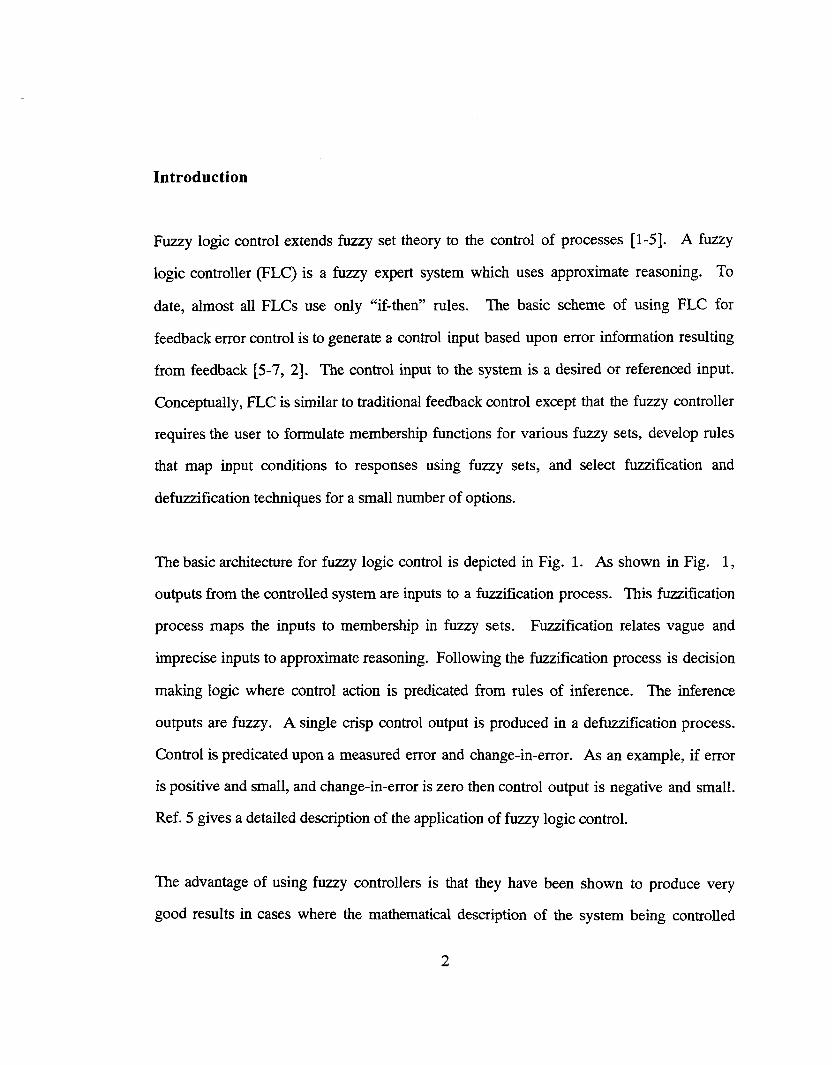
The basic architecture for fuzzy logic control is depicted in Fig. 1. As shown in Fig. 1,

outputs from the controlled system are inputs to a fuzzification process. This fuzzification

process maps the inputs to membership in fuzzy sets. Fuzzification relates vague and

imprecise inputs to approximate reasoning. Following the fuzzification process is decision

making logic where control action is predicated from rules of inference. The inference

outputs are fuzzy. A single crisp control output is produced in a defuzzification process.

Control is predicated upon a measured error and change-in-error. As an example, if error

is positive and small, and change-in-error is zero then control output is negative and small.

Ref. 5 gives a detailed description of the application of fuzzy logic control.

The advantage of using fuzzy controllers is that they have been shown to produce very

good results in cases where the mathematical description of the system being controlled

2

may not be readily available or the description may be of questionable fidelity [8-131.

Despite the use of simple fuzzy logic control, there are specific drawbacks [12, 141 due to

tuning the controllers to meet some performance objective.

Methods for tuning fuzzy controllers include using neural networks, fuzzy self-organizing

control (SOC), genetic algorithms, and human knowledge. The SOC is essentially a

decision maker predicated upon performance feedback. The SOC is capable of generating

and modifying the control rules based upon an evaluation of their performance. The SOC

is composed of three elements: performance index evaluation, credit assignment, and rule

modification. The performance index and credit assignment require a priori knowledge of

desired controller input-output mapping. Daley and Gill [ 12,141 have demonstrated the use

of SOC for the attitude control of a spacecraft.

Neural Networks have also been used because of their learning capabilities for system

identification and/or tuning. However, simultaneous tuning of membership functions and

identification of inference rules is difficult. Rules identified by networks are difficult to

understand. Furthermore, training neural networks is computationally time consuming.

Genetic algorithms are a form of directed random search. To implement genetic

algorithms, the fuzzy sets must be parameterize discretely. The discrete set forms an initial

population for the genetic algorithm. The population evolves to produce new, but

hopefully better design of the fuzzy sets. Human knowledge can be used to tune the

controllers. However, such knowledge must be developed into a reliable linguistic model

of an operator’s strategy. Another consideration for using user knowledge is that the

system processes may change beyond the operator’s realm of experience.

3

This paper presents a new approach for tuning fuzzy logic controllers using numerical

optimization. The main attribute of this approach is that it allows fuby logic controllers to

be tuned to achieve global performance requirements. Furthermore, this approach allows

design constraints to be implemented during the tuning process. The approach consists of

specifying the desired outcome of tuning a fuzzy controller (e&, system time response) as

minimization of an objective function. The control design methodology is applied to a

spacecraft mounted science instrument (payload) which rotates about a drive shaft. The

design goal is to have a bounded response amplitude while having the instrument meet

mission pointing requirements. Fuzzy logic control is used as a means to maintain either a

constant slew rate or fixed line-of-sight pointing for the payload subjected to vibration due

to multiple disturbance sources.

Design constraints such as physical limitations in hardware or software such as controller

torque output (magnitude vs. frequency), measurement sampling rate, measurement

sampling range (Le., limits), etc. can be included in the optimization process and fuzzy

logic controller development. Fuzzy membership support limits are naturally malleable to

some system specifications such as error measurement range and control output. If prior

knowledge of the controller's maximum output and measurement range (error and error

rate) is available, a fuzzy logic controller can be tuned by having the control support limit

as the controller's output maximum value. The error support limitation could be either the

physical measurement limit or it could reflect a bound of measurement within a given

regime of operation. paper allows for

constraints to be included in the tuning process either in the constraint equations or with the

upper and lower bounds on the design vector.

The design methodology presented in this

4

Optimization Strategy - General

An objective function is prescribed such that, as it is reduced in value, the overall

performance improves. Furthermore, the objective must be explicitly or implicitly

dependent upon a set of design parameters. Design parameters are given such that they can

be varied to change the overall performance (design objective). Thus, the design objective

is to minimize

subject to

F ( a )

Gj(a) 5 0 j = I,m

and

a[, 5 ai 5 au, i = 1,n

( 2)

whereF(a) is an objective function which, when minimized, will result in optimum

performance of the system. The vector, a, contains n system parameters which are varied

through the iterative optimization process. Gj(a) is the jth constraint on the design

parameters. There are m constraints. Each design parameter, ai , is bounded by upper

and lower limits, aIi and aUi , respectively.

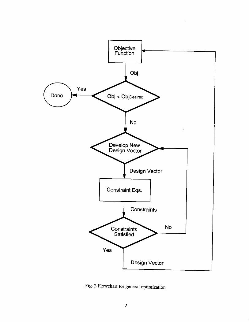
A flowchart of the optimization procedure is shown in Fig. 2. The procedure is iterative.

The first iteration requires the user to develop an optimization objective, constraint

equations, and bounds for the elements of the design vector. In the first iteration, the

objective function is evaluated. If the objective value is less than some desired value, the

process is complete. If the objective value is greater than some desired value, the

5

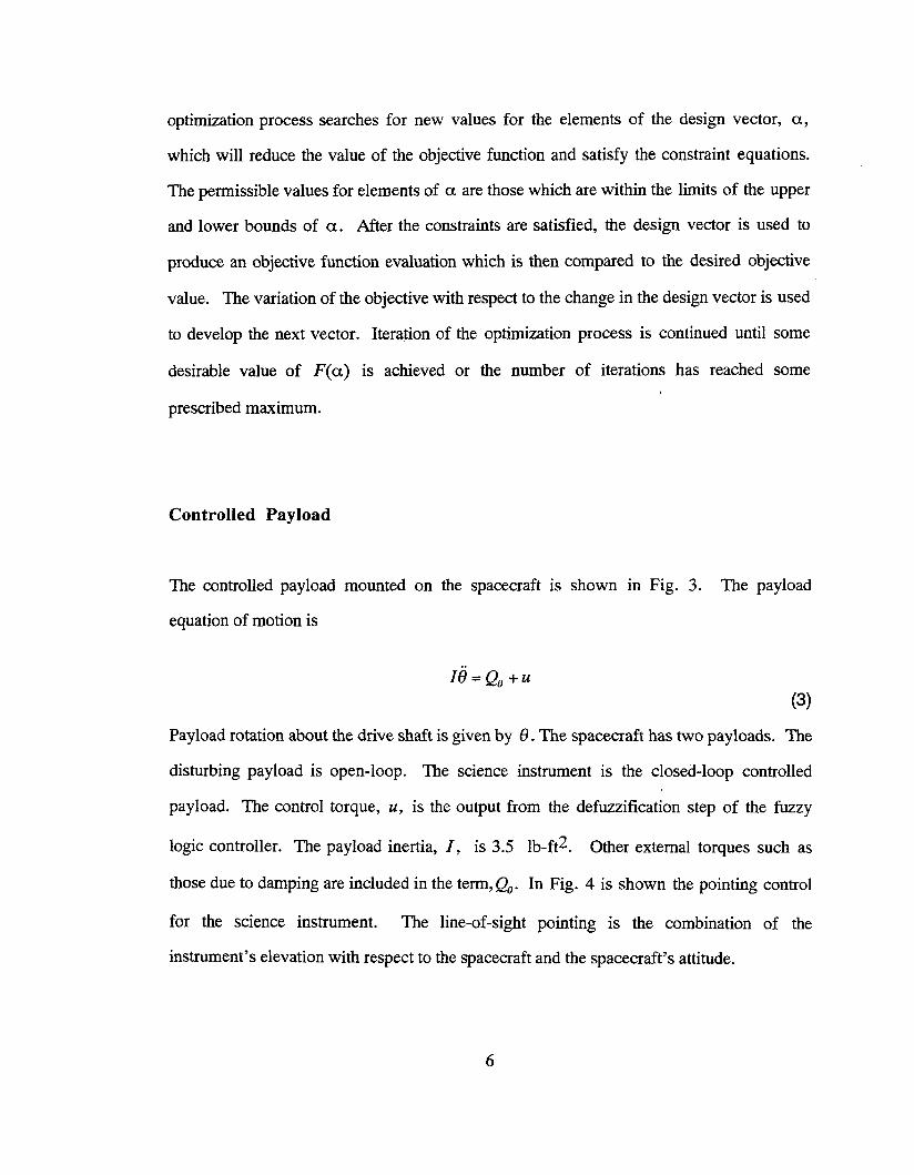
optimization process searches for new values for the elements of the design vector, a,

which will reduce the value of the objective function and satisfy the constraint equations.

The permissible values for elements of a are those which are within the limits of the upper

and lower bounds of a. After the constraints are satisfied, the design vector is used to

produce an objective function evaluation which is then compared to the desired objective

value. The variation of the objective with respect to the change in the design vector is used

to develop the next vector. Iteration of the optimization process is continued until some

desirable value of F(a) is achieved or the number of iterations has reached some

prescribed maximum.

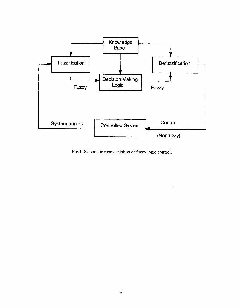
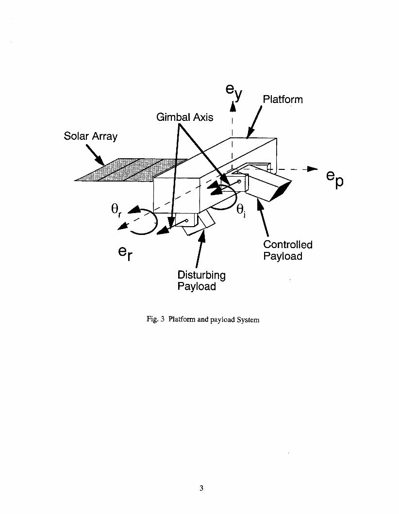
Controlled Payload

The controlled payload mounted on the spacecraft is shown in Fig. 3.

equation of motion is

The payload

I ~ = Q ~ + u (3)

Payload rotation about the drive shaft is given by 8. The spacecraft has two payloads. The

disturbing payload is open-loop. The science instrument is the closed-loop controlled

payload. The control torque, u, is the output from the defuzzification step of the fuzzy

logic controller. The payload inertia, I , is 3.5 lb-ft2. Other external torques such as

those due to damping are included in the term, Qe. In Fig. 4 is shown the pointing control

for the science instrument.

instrument’s elevation with respect to the spacecraft and the spacecraft’s attitude.

The line-of-sight pointing is the combination of the

6

Fuzzy Logic Control

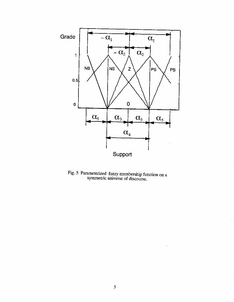
In Fig. 5 is shown a parameterized fuzzy membership function. The same membership

functions are used for the error, change-in-error, and control output. The fuzzy term sets

are positive big, (PB), positive small, (PS), zero, ( Z ) , negative small, (NS), and

negative big, (NB). These sets are symmetric about zero and are bounded by a parameter,

a,, which defines minimum and maximum support limits. Positive small, (ps), and

negative small, (NS), singletons (membership has a grade of 1.0) are located on the

universe of dkcourse by a2. The base for the triangular membership function zero, ( z ) , is defined by a,; negative small, (NS), and positive small, (PSI, bases are defined by

a4; and, the negative big, (NB), and positive big, (PB), bases are defined by a,. The

initial membership functions (first optimization step) have an overlap at grade 0.65. This

overlap gives all support elements membership in two term sets unless the support element

has membership grade of 1.0 in any term set. Because of the overlap, the control gradient

with respect to the error and change-in-error is continuous, monotonic, and never zero

[13]. The advantage this fuzzy membership offers is the effect that the membership

functions have when the support elements are near zero. Unless the element is absolutely

zero, the elements have nonzero grades on the respective side of zero. The result is a

smooth approach to zero for process output as the support elements approach zero. The

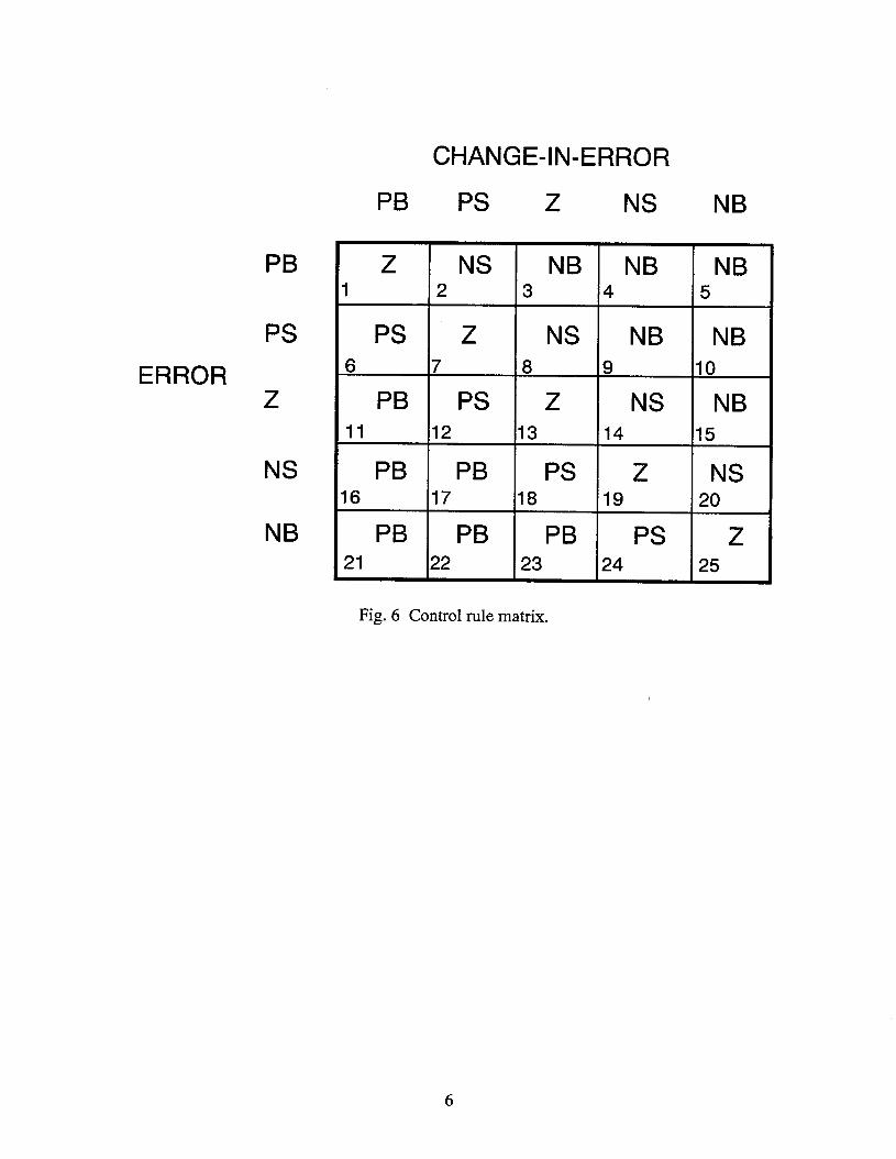
membership functions depicted in Fig. 5 are used for the payload error, change-in-error

and control. The control rule matrix used is shown in Fig. 6. Each element of the matrix

is numbered and corresponds to a rule. For example, Rule 7 states that if error is PS and

change-in-error is NS then the control output should be 2.

7

Optimization Strategy for Controller Design

In this paper, the objective is derived from the system response. The optimization design

objective, F ( a ) , is to minimize the aggregate square of error between a measured position

and commanded position. Thus

where x(a,t) is the measured position at time t and xcom is the commanded position. The

design vector, a, has three sets of parameters, al, # * e , a5, for a total of 15 elements.

Each membership function uses the following constraint to maintain the ordering of the set

terms:

G,(a) = 1 .25a2 - a,

The following constraints assure continuous mapping from error and change-in-error to the

control output. The constraints also assure overlap of adjacent membership functions.

Because of the overlap, the control gradient with respect to the error and change-in-error is

continuous, monotonic, and never zero.

8

G2(a) = (a, - as) * 1.10 - (a2 + a,)

G3(c1) = -a3 + (az - ag) * 1.10

A constraint is violated if

G j ( a ) =- 0

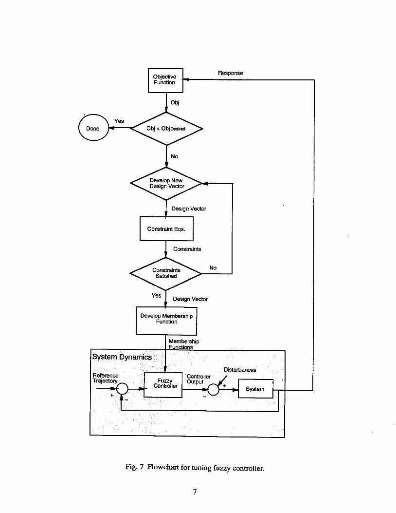
The flowchart for tuning the fuzzy controller is shown in Fig. 7. The general optimization

procedure mentioned earlier is uesd. However, the design vector is used to generate the

fuzzy logic membership functions. The system produces another response with the

member functions. The new response is used to generate a new objective function

evaluation.

The instrument fuzzy controller has three modes of operation: slew maneuvers, disturbance

rejection (impulse and periodic vibration) and trajectory tracking. To demonstrate the

methodology, the instrument controller will be tuned to perform slew maneuvers and

disturbance rejection using the same initial design parameters. The initial design parameters

were chosen such that they produce unsatisfactory system response. Successive iterations

of the optimization process will reduce the objective function. The iterations terminate

when a set of design parameters, a, is generated which will produce a desired objective,

F ( a ) .

9

Numerical optimization was performed using the Automated Design Synthesis (ADS)

software [15]. The method of feasible directions for constrained minimization with

sequential quadratic programming is used for optimization. In Figs. 8 through 10 are the

initial and final membership functions for error, change-in-error, and control that were

generated while tuning the instrument controller for a 0.5 radian slew maneuver. The

membership functions for all term sets changed during the design process. However,

changes for zero, 2, were not as pronounced. The support limits for error, change-in-

error and control changed from 0.1, 0.01, 0.01 to 0.12, 0.037, 0.064, respectively. An

iteration history of the normalized objective (normalized to the objective evaluated during

the first iteration) is shown in Fig. 11. The objective function was reduced to 1% of that

evaluated for the first iteration after 60 iterations. The final (tuned) fuzzy controller

produced a response which achieved the desired position in 23 sec. without overshoot, as

shown in Fig. 12. After 40 sec., the response using the initial controller did not reach the

desired commanded position of 0.5 rad.

In Figs. 13 and 14, are shown the results of tuning the instrument fuzzy controller while

the instrument is commanded to maintain a position of 0.0 rad. in the presence of a periodic

disturbance (amplitude = 0.Olft-lb and frequency = 0.25 Hz). The objective function,

F(a) , is reduced to 1% of the initial function after 27 iteration steps (Fig. 13). In Fig. 14

is shown the response for the initial and final controllers. The initial response amplitude is

approximately 0.005 rad. The final response amplitude has' been reduced to

approximately 0.00005 rad.

10

Tracking Controller Development

The results presented thus far have shown the capability of tuning a fuzzy controller by

parameterizing the membership functions and then using the parameters in a numerical

optimization algorithm. The same initial membership functions were used in all cases.

Reduction to 1% of initial objective function was used as the criterion for terminating the

optimization process. In all cases, the final responses were satisfactory. The initial

membership functions demonstrated the effectiveness of using numerical optimization to

tune the controllers. The following discussion demonstrates that the approach can be used

to enhance the tuning of controllers which already exhibit satisfactory performance.

A common need of many space-based payloads is the requirement to track a target,

reposition, and track another target. Such retargeting occurs when communication

antennae track relay satellites. The instrument controller was tuned by parametrically

varying support limits for error, change-in-error, and, control output. The final design,

arrived at in Ref. 16, is used as an initial design in the optimization process. The

optimization design objective, F ( a ) , is to minimize the aggregate square of error between a

measured trajectory and desired trajectory. Thus

where xd(t ) is the desired trajectory. After 71 design iterations, the objective function is

reduced to 1% of its initial value. In Fig. 15a is shown the commanded elevation for the

11

instrument to track. The results of using the initial and final designs are shown in Fig.

15b. The initial design has a tracking error greater than 0.25 rad. The final design of the

fuzzy controller significantly tracks its commanded position better with a tracking error

less than 0.01 rad.

Concluding Remarks

This paper has presented the development and viability of a method to tune fuzzy

controllers using numerical optimization. A spacecraft science instrument pointing control

model was used to demonstrate the application of the methodology. The optimization

approach allows a designer to tune membership functions for all linguistic variables to

achieve global performance. Furthermore, this approach allows design constraints to be

implemented during the tuning process.

The optimization approach consists of specifying the desired outcome of tuning a fuzzy

controller (e.g., system time response) as minimization of an objective function. The

objective function is prescribed such that, as it is reduced in value, the overall performance

improves. Furthermore, the objective must be explicitly or implicitly dependent upon a set

of design parameters. Design parameters are given such that they can be varied to change

the overall performance (design objective).

The controller was tuned by parameterizing the membership functions. The resulting

parameters formed a design vector which was used in the iterative numerical optimization

process. Optimization objectives used included minimizing the aggregate square of error

between a measured position and commanded position; minimizing the aggregate absolute

12

error between a measured position and commanded position; and minimizing the aggregate

square of error between a measured trajectory and desired trajectory. In the design cases

presented, the objective was reduced to 1% of its initial value within 80 optimization

iterations.

Instrument design results included tuning the controller for 0.5 rad slew maneuver,

disturbance rejection (impulse and periodic), and trajectory following. In tuning for the

slew maneuver, the support limits for error, change-in-error, and control changed from

0.1, 0.01, 0.01, to 0.12, 0.037, 0.064, respectively. Using the final design, the

instrument completed the maneuver in 23 sec. without overshoot. The final instrument

controller design tuned for disturbance rejection when the instrument was subjected to a

periodic disturbance resulted in a final response which reduced to 0.00005 rad (initial

response was 0.005 rad). When subjected to unit impulse, the final instrument design was

stable with a settling time of 21 sec. The final design used for tracking a trajectory reduced

the tracking error to 0.01 rad (initial tracking error was 0.25 rad).

13

References

[l] Turksen, I. B., “Rule and Operation Decompositions in CRI,” Advances in Fuzzy Theory and Technology , Edited by P. P. Wang, Bookwrights Press, Durham, North Carolina, 1993, pp. 219-256.

[2] Zadeh, L., “Fuzzy Logic,” Computer, Computer Society of the IEEE, Vol. 21, April

[3] Smith, K. C., “Multiple-valued Logic: A Tutorial and Appreciation,” Computer, Computer Society of the IEEE, Vol. 21, April 1988, pp. 17-27.

[4] Aldridge, J., “Terminology and Concepts of Central and Fuzzy Logic,” Proceedings of the AIAA Guidance, Navigation and Control Conference, New Orleans, Louisiana, August

1988, pp. 83-93.

12-14, 1991.

[5] Woodard, S. E., “Concurrent Fuzzy Logic Control of a Gimballed Payload and Space Spacecraft System,” Ph.D. Paper, Dept. of Mechanical Engineering and Materials Science, Duke Univ., Durham, NC, Dec. 1995.

[6] Lee, C. C., “Fuzzy Logic in Control Systems: Fuzzy Logic Controller - Part 1,” IEEE Transactions on Systems, Man and Cybernetics, Vol. 20, No. 2, MarcWApril 1990, pp. 404-418.

[7] Lee, C. C., “Fuzzy Logic in Control Systems: Fuzzy Logic Controller - Part 2,” IEEE Transactions on Systems, Man and Cybernetics, Vol. 20, No. 2, MarcWApril 1990, pp. 419-435.

[SI Cunningham, G. B., Horstkotte, E. A., and Bochsler, D. C., “Integrating Fuzzy Logic Technology into Control Systems,” Proceedings of the A I M Guidance, Navigation and Control Conference, New Orleans, Louisiana, August 12-14, 1991, pp. 1699-1702.

[9] Schwartz, D. G., “Japanese Advances in Fuzzy Systems and Case-Based Reasoning,” National Technical Information Service, No. PB92-115443, November 1991.

[ 101 Hirota, K., “Research Activities and Industrial Applications of Fuzzy Technology in Japan,” Advances in Fuzzy Theory and Technology, Edited by P. P. Wang, Bookwwrights Press, Durham, North Carolina, 1993, pp. 269-282.

[ll] Lea, R. N. and Jani, Y., “Fuzzy Logic in Autonomous Orbital Operations,” Proceedings of the Second Joint Technology Workshop on Neural Networks and Fuzzy Logic, Volume 2, NASA Conference Publication 10061, February 1991, pp. 81-110.

[12] Daley, S. and Gill, K. F., “Comparison of a Fuzzy Logic Controller with a P + D Control Law,” Journal of Dynamic Systems, Measurements, and Control, Vol. 11 1, June 1989, pp. 128-137,

14

[13] Aldrige, J., Yashvant, J., and Zafar, T., “Tuning Fuzzy Cqntrollers for Electric Motors,” Proceedings of the Third International Symposium on Measurement and Controls in Robotics, Torino, Italy, September 21-24, 1993, pp. 1-49 to 1-53.

[14] Daley, S. and Gill, K. F., “Attitude Control of a Spacecraft Using an Extended Self- Organizing Fuzzy Logic Controller,” Proceedings of the Institution of Mechanical Engineers, Part C , Vol. 201, No. C2, 1987, pp. 97-106.

[15] Vanderplaats, G. N., “Automated Design Synthesis (ADS) - A FORTRAN Program for Automated Design Synthesis,” Version 1.10, NASA CR 177985, September 1985.

[16] Woodard, S . E., Garg, D. P., Tyan, C. Y., and Wang, P. P., ” An Application of Fuzzy Logic Control to a Gimballed Payload on a Space Spacecraft,” Journal of Information Sciences- Applications, November 1995, Vol. 4, No. 3. pp 143-166.

15

~~ Knowledge Base

Fig.1 Schematic representation of fuzzy logic control.

_c. Fuzzification

1

Def uzzif ication -

Fuzzy Fuzzy Logic

System ouputs Control Controlled System

Objective Function

Constraint Eqs. I

1

?ctor

Design Vector

Fig. 2 Flowchart for general optimization.

2

Gimbal Axis

Disturbing Payload

Fig. 3 Platform and payload System

3

Spacecratt Attitude

Reterence - Elevation 6-I F:$lfnt Controler t

I - Control nstrument

Torque ~ Instrument e :levation

I I U' t -

Fig. 4 Spacecraft mounted instrument pointing control.

4

Grade

1

0.5

0 'Y 1

I + support

Fig. 5 Parameterized fuzzy membership function on a symmetric universe of discourse.

5

CHANGE-IN-ERROR

Z

PS

PB

PB

PB

1

6

11

16

21

PB NS NB

Z NS

PS Z

PB PS

PB PB

2 3

7 8

12 13

17 18

22 23

PS

NB 4

ERROR

~~

NB 5

Z

NB

NS

Z

9

14

19 NS

~

NB

NB

NS

10

15

20

NB PS 24

PB PS Z

Z 25

NS NB

Fig. 6 Control rule matrix.

6

Objective Function I

I

Response -1

1 No

Develop New Design Vector

Constraint Eqs.

Constraints

Satisfied

yes 1 Designvector

Develop Membership Function

Disturbances

Fig. 7 Flowchart for tuning fuzzy controller.

7

Initial Error Membership Functions 1 I I I I I 1

Grade 1.0

0.0

NB NS Z PS PB - - -

- - -

Grade 1.0

0.0

Fig. 8 Initial and final payload error membership function for slew maneuvers.

I I I I I

NB NS Z PS PB - - -

- - - -

8

Initial Change-In-Error Membership Functions

1.0

0.0

I NB NS Z PS PB -

- - -

~ I I

m0.03 -0.02 -0.01 0 0.01 0.02 0.03 0.04

Final Change-In-Error Membership Functions Gr

" I I

-0.01 0 0.01 0.02 0.03 0.04

Change- I n - Error S u p PO rt (Rad i a n s)

Fig. 9 Initial and final change-in-error membership function for slew maneuver.

9

Grade 1.0

0.0

Final Control Membership Functions

I I I I I I I

NB NS Z PS PB - -

- - - -

I I I I

Grade 1.0

0.0

Control Output Support (Ft-LB)

I I I I I I I

NB NS Z PS PB - - -

-

- - - - -

Fig. 10 Initial and final payload control membership function for slew maneuvers.

10

I I I I I I I 1 I

1.4

0.0 I

1.21 Normalized

- I I I I I I

P Objective

0.8

0.6-

0.4

0.2

-

-

-

iteration Step

Fig. 11 Normalized payload objective iteration history resulting from tuning for slew maneuver.

11

Position (Radians)

Time (Sec.)

Fig. 12 Payload response to a commanded slew of 0.5 rad. using initial and final membership functions.

12

Normalized Objective

0.0

1.4

I I I I I

1.2

1 .c

0.8

0.6

0.4

0.2

I I I I I I I

Fig. 13 Normalized payload objective iteration history while tuning for periodic disturbance rejection (0.01 ft-lb., 0.25 Hz.)

13

Position (Radians)

Time (Sec.)

Fig. 14 Payload response to a periodic disturbance (0.01 ft-lb., 0.25 Hz ) using initial and final membership functions.

14