A NUMERICAL MODEL OF THE MOTION OF A CURVED FLEXIBLE FIBRE IN A SHEAR FLOW

Inna Galperin

A thesis submitted in conformity with the requirements for the degree of Master of Applied Science

Graduate Department of Chernical Engineering and AppIied Chemistry University of Toronto

O Copyright by Inna Galperin 1997

395 Wellington Street 395, rue Wellington Ottawa O N K I A ON4 Ottawa ON K1A ON4 Canada Canada

The author has granted a non- exclusive licence allowing the National Libraq of Canada to reproduce, loan, distribute or sel1 copies of this thesis in microfom, paper or electronic formats.

The author retains ownership of the copyright in ths thesis. Neither the thesis nor substantial extracts fkom it may be printed or otherwise reproduced without the author's permission.

Your file Vorre réference

Our Iris Notre réfdrence

L'auteur a accordé une licence non exclusive permettant à la Bibliothèque nationale du Canada de reproduire, prêter, distribuer ou vendre des copies de cette thèse sous la forme de microfiche/film, de reproduction sur papier ou sur format électronique.

L'auteur conserve la propriété du droit d'auteur qui protège cette thèse. Ni la thèse ni des extraits substantiels de celle-ci ne doivent être imprimés ou autrement reproduits sans son autorisation.

Inna GaIperin, M. A. Sc., 1997

Department of Chernical Engineering and Applied Chemistry University of Toronto

Abstract

A general method to simulate the motion of initially curled flexible fibres in 2-D

flows is developed. Equations of motion are formulated for a curled, elastic fibre in a fluid

flow using Hamilton's Principle. The non-linear integro-differentid equations contain an

unknown deflection variable that is discretized using a half-range Fourier Sine series

representation. The first (kincmatic) approximation is obtained by setting the inertia terms

to zero. The resulting inertialess equations are solved using a Runge-Kutta method

irnplemented in a C++ code.

The validity of the numerical model was tested against analytic theory and existing

transient results for essentially straight fibres, i.e. fibres with smdl radii of curvature and

large angles. Excellent agreement was achieved. The numericd model was then applied to

simulate fibre motion into a screen slot. For similar fibre parameters, it was found that

significantly more curled fibres entered the slot than their straight counterparts.

Acknowledgments

1 am greatly indebted to Professor D. C. S. Kuhn for his supervision and guidance

throughout the duration of my thesis. 1 would also Iike to thmk everyone associated with

the Pulp and Paper Centre for allowing me the opportunity to hone my research skills and

to participate in the technology tour and the conferences that have contributed very much

to my learning experience.

1 would like to acknowledge Yuri Lawryshyn for his input and advice, and

Abitibi-Consolidated for providing a workplace when 1 needed it. Many thanks to my

colleagues for their help and for a pleasant working environment. 1 would also like to

thank my friends here in Toronto for their good attitude and for the necessary social

distractions that have made my work and stay a valuable personal experience.

Finally, 1 would like to express my gratitude to my parents, sister, and grandfather

for their warmth, kindness and support, both in work, and in life.

Abstract

Acknowledgments

Table of Contents

1 Introduction

2 Literature Review

2.1 Previous Fibre Flow Models

2.2 Harrnonic Analysis

2.3 Fluid Forces

2.4 Application to Pulp Screening

3 Mathematical Model

3.1 Fibre Model

3.2 Hamilton's Principle

3.2.1 Kinetic Energy

3.2.2 Potential Energy

3.2.3 Virtual Work

3.3 Exact Integro-Differential Equations of Motion

4 Orthogonal Expansion of Deflection Function

4.1 Circular Ring

4.2 Circular Arc

5 Kinematic Inertialess Equations

5.1 First Kinematic Approximation

ii

iii

6 Numerical Model

6.1 Runge-Kutta Method

6.2 Computational Algorithm

7 Model Validation and Applications

7.1 Model Validation

7.1. I Static Analysis

7.1.2 Dynamic Curved Fibre Motion

7.1.3 Results and Discussion

7.2 Fibre Motion into Slot

7.2.1 Fibre Passage Values: Hfcrit

7.2.2 Discussion of Results

7.2.3 Application to Pulp Screening

8 Concluding Remarks

8.1 Surnmary of Numerical Model

8.2 Applications

8.3 Suggested Future Work

9 References

A Inertialess Equations for m = 3 Modes of Motion

Chapter 1

Introduction

Many business, commercial, and academic enterprises need high quality paper of

good strength, printability, and optical properties. Thus, fibre quality, in particular fibre

flexibility, is an important concem for the pulp and paper industry. It is generally believed

that longer, more flexible fibres have superior bonding characteristics to their shorter, stiffer

counterparts, and thus contribute to better paper quality. Pulp screening processes attempt to

separate or fractionate short, stiff fibres, and shives from the more desirable flexible ones.

Shives are unseparated fibre bundles that give rise to uneven paper morphology, and can

adversely affect the printability and optical properties of paper. In addition, shives may

accumulate stress concentrations which can contribute to poor paper strength.

The prior work of Lawryshyn and Kuhn [27] examined the Flow of an individual

fibre by modeling it as a flexible cylinder with straight initial shape. Howevcr, due to

various chernical and mechanical processes that fibres tend to undergo during papermaking,

many fibres assume a curled initial shape (see Page et al. [35]) . Thus, the goal of this

motion of an initially curled flexible fibre in a shear flow. Equations of motion are

developed for a curled flexible fibre and are subsequently solved by existing numerical

methods and compared to prior results. Throughout the formulation of the equations, small

deflection theory is assumed and the fluid forces acting on the fibre are estimated based on

the first order approximations of Cox [6 j.

The equations of motion are non-linear and integro-differential in form, containing

an unknown deflection variable. The deflection variable is represented as a function and

discretized by the Rayleigh-Ritz assumed modes method. A C++ implemented Runge-Kutta

routine solves for the time parameters of the unknown deflection function. Ln the test case,

the sme shear flow and fibre parameters are used as those ernployed for the straight fibre

case to allow for cornparison to prior theoretical and computational results. This new curled

fibre analysis is then applied to consider the motion of fibres in a channel flow with a dot,

i.e. a simplified screen geometry.

Chapter 2 presents a literature review encompassing the topics discussed in this thesis.

Chapter 3 presents the analytical work used to formulate the equations of motion. Chapter 4

proposes an orthogonal expansion for the unknown deflection function. The poverning

equations, capable of describing the full motion and deflection of a curled, flexible fibre are

simplified to the inertialess case in Chapter 5. Chapter 6 presents the numerical procedure

and the algorithm used to dynamically solve the mathematical model. Comparison to prior

results and applications of the model are presented in Chapter 7 . Chapter 8 discusses the

thesis are presented in the appendix.

Chapter 2

Literature Review

Previous fibre flow models of Gooding [15], Kumar [25], Olson [34], and

Lawryshyn [26], examine the flow of fibres through narrow apertures. Kumar and

Gooding's models are experimental and study the effect of fibre, flow, and slot parameters

on fibre passage through slot geometries. Olson, and Lawryshyn's models are of a

theoreticai nature, and model fibre passage through narrow apertures. Al1 four models are

discussed in the first section.

This thesis presents a mathematical and numerical mode1 for the motion of a curled

flexible fibre in pulp flow, with applications to the study of pulp screening. Fundamentals of

mathematics and geometry found in many textbooks such as Stewart [48] and [49], were

used to arrive at a fibre model. Hamilton's Principle (Meirovitch [30]), used to formulate

the equations of motion, required representations for the energy expressions, a topic found in

standard dynamics texts like Meriarn [32]. The resulting integro-differential equations of

motion contain an unknown deflection variable, as well as a general representation for the

Harmonic analysis, a topic found in rnany texts (e.g. Greenberg [18]), is outlined in the

second section and was used to discretize the deflection function. Cox's [6 ] first

approximation is used for the fluid forces and is presented in the second section. The fourth

section comprises a general discussion on pulp screening.

2.1 Previous Fibre Flow Models

Kumar' s [25] largely experimental approach studied the ability of aqueous fibre

suspensions to penetrate a single aperture located in a flow channel as well as multiple

apertures in a device simulating a commercial pulp screen cross-section. The flow

conditions used approximated that of commercial screening processes which have a large

channel velocity compared to the aperture velocity. The aperture dimensions were greater

than a fibre's diameter, but Iess than a fibre's length. Kurnar's experimentaI measurements

of fibre passage were related to a ratio of fibre length to aperture width (WW) for both stiff

and flexible fibres.

Gooding's [ 1 51 experimental approach examined the influence of fibre, flow, and

slot variables on fibre passage through an aperture. He found that reduced fibre stiffness and

length increase fibre entry. Gooding also obtained images of fibre trajectories through high

speed ciné-photography. He observed two effects: the "wall effect" whereby a layer of flow

that passes through the dot is depleted of large fibres, and an "entry effect" where short,

findings suggest that shorter or more flexible fibres pass through an aperture more reridily

than longer or stiffer fibres.

Olson 1341 developed a theoretical model to determine the passage ratio of stiff fibres

of 1, 2, and 3 mm lengths through narrow apertures. His model made use of the wail effect

and the turning effect witnessed by Gooding. Olson's mode1 was compatible to prior

experimental results.

Lawryshyn's [26] theoretical model studied the static and dynamic behavior of pulp

fibres. He modeled the flow of initially straight, flexible fibres through small apertures by

developing a set of non-Iinear integro-differential equations of motion. Lawryshyn's

theoretical mode1 was found to agree with static deflection beam theory.

2.2 Harrnonic Analysis

Al1 bodies having mass and elasticity are capable of vibration. There are two classes

of vibration: free vibration and forced vibration. Free vibration t'îkes place under the

absence of external excitation, whereas forced vibration occurs under excitation by external

forces. In free vibration, the body oscillates under the action of forces inherent in the system

itself. A thorough discussion of these topics c m be found in Thomson [52].

motion, wil1 oscillate at one or more of its natural frequencies in free vibration. Oscillations

may repeat themselves regularly or irregularly. Oscillatory motion repeated rit regular time

intervais is known as periodic motion, with the time interval T called the period of

oscillation.

The simplest form of periodic motion is harrnonic motion. In harmonic motion, the

acceleration is proportional and opposite to the displacement and can be characterized solely

by sine and cosine terms. In multi-degree-of-freedom systems, vibrations of several

different frequencies can exist simultaneously resulting in a complex waveform that is

repeated periodically as s hown in Figure 2.2- 1.

Figure 2.2-1. Complex Periodic Waveform.

of sine and cosine terms. Thus a general periodic function x(t) of period r c m be

represented by the Fourier series:

where

The deflection variable in the mathematical model can be approximated by a

deflection function and discretized by the Rayleigh-Ritz method (see Meirovitch [30]). A

Fourier expansion is used for the deflection function; this topic is treated extensively in the

literature (e.g. Greenberg [ 183).

2.3 FIuid Forces

The numerical model of Chapter 6 develops the kinernütic inertialess equations.

These equations require an explicit formulation for the fluid forces acting on the fibre.

Several approxi mate analyticril solutions for the hydrodynarnic forces acting on a long,

slender body are available in the literature. Cox [6] developed expressions for the flriid force

was taken to be negligible. Batchelor [Il calculated the resultant fluid force and couple

required to sustain translational and rotational motion in a straight, rigid slender body. De

Mestre [IO] presented low-Reynolds number results for the drag and torque on a rigid

slender cylinder translating near a plane wall. Recent work by Khayat and Cox [22],

extended [6] and [7] by formulating equations for the fluid force and torque acting on a

slender body with non-negligible fluid inertia. In the lirniting case of 1ow Reynolds nurnber,

the results for both cases were found to agree. This work will use Cox's first order

approximation for the normal and tangential fluid force per unit length acting on the body as

where

p is the viscosity of water,

Un and Ut are the normal and tangential components of the fluid velocity,

V,, and are the normal and tangential cornponents of the fibre velocity,

L is the fibre length,

2.4 Application to Pulp Screening

Previous work on the topic of pulp screening has been both experimental and

niinerical in nature. Gooding [15] and Kurnar [25] studied the passage of aqueous fibre

suspensions through an aperture or slot geometry. Because the aperture width is larger than

the minimum diameter of many shives, Kumar concluded that the screening process does not

rely on physical obstruction but rather on unknown mechanisms and fibre properties such as

fibre flexibility. Gooding, in characterizing a wall and an entry effect, found that shorter

andor more flexible fibres enter the aperture more readily. Thus, both Gooding and

Kumar's experimental approach showed the importance of fibre flexibility in the passage of

fibres through narrow apertures.

By approximating flow conditions similx to pulp screening, Olson [34] examined

the passage of fibres through narrow apertures by developing a theoretical mode1 for the

motion of rigid fibres entering a dot. Lawryshyn (261 studied the motion of an irzitirilly

strnight flexible fibre in a channel flow with a slot, and examined the effect of fibre

flexibility. His mode1 proved the occurrence of pulp screening based on fibre flexibility. To

date, no known mode1 of the motion of iizitinlly ccrrled flexible fibres in channel and slot

geometries is known to exist. In view of the fact that many fibres produced through the

of pulp screening.

Chapter 3

Mathematical Model

The equations governing the motion of a curved flexible fibre in a 2-D plane are

developed in this chapter. The curved fibre is modeled as a cylinder of a given flexibility

with curved initial shape, and the exact equations of motion for the fibre are developed using

Hamilton's Principle. The proposed mode1 expands upon the specific case of a straight,

flexible fibre considered by Lawryshyn and Kuhn [27] to the more general case of a curved

flexible fibre.

3.1 Fibre Model

A curled fibre is modeled as an arc of a circle of constant radius of curvature r'.

Figure 3.1 - 1 shows the coordinate systems and the magnified geometry of a deflected curved

fibre, where X, Y are absolute coordinates; x, y are relative coordinates; Ir1 = constant; 6 is

' From this point forward, the term "curved" fibre will be used to describe a "curled" fibre.

are considered.

Figure 3.1-1. Geometry and coordinate systems of a typical curved fibre.

The position vector R of any point on the fibre is thus given by

where Ro is the position vector of the origin of the relative coordinate system x-y, r and a are

location parameters, u ( a t ) is the deflection of the fibre at a point defined by the polar

coordinates r and a. The projection of (3.1) ont0 the X and Y axes yields

Here, the variables Xo, Yo, u and 8 depend on time t, and define the absolute motion of a

fibre. Taking the time derivative of equation (3.2) yields

where R is the time derivative of R.

3.2 Hamilton's Principle

There exist various methods of forrnulating the equations of motion. Newtonian

mechanics uses Newton's second law, F = ma , to derive the equations of motion in terms of

vector quantities for each mass separately. As implied by the equation, forces appear

explicitly in Newtonian rnechanics, see for example Meriam [32]. Analytical mechanics

uses scalar quantities, namely the kinetic and potentiai energies and the virtual work, instead

of vectors to formulate the equations of motion. This approach is especially useful and very

powerful when describing systems of more than one particle, and distributed mass systems

such as a fibre in a fluid. Within analytical mechanics, many representations are possible

such as the Lagrangian formulation, or Hamilton's principle (Meirovitch [30]). The

used, but the Lagrange equations make use of generalized forces, whereas HamiIton's

principle does not. Because of the difficulty of identifying generalized forces in our

analysis, Hamilton's principle is used in this application.

Hamilton's principle is a way of formulating the equations of motion using the scalar

quantities of kinetic and potential energies and the virtual work for a systern moving along a

varied path. A systern of particles travels dong the varied path Ri ( t ) + GRi ( t ) made up of

the true path Ri( t ) and the virtual displacements 6 R i ( t ) , which are possible imaginary

displacements respecting constraints at frozen time. The varied path is chosen such that it

coincides with the true path at the two times t = t , and t = t 2 , implying that

SRi ( t , ) = 6Ri ( t , ) = O . Hamilton's principle rnay thus be represented as [30];

where ST is the variation in kinetic energy,

m/ is the variation in potential energy,

SW is the virtual work,

6Ri ( t ) is the variation from the true path, or the virtual displacement at frozen tirne.

energy, and the virtual work.

3.2.1 Kinetic Energy

The kinetic energy of the fibre system is

where dm is the elementary mass and L is the length of a fibre. Denoting v = volume, p =

constant density, A = constant cross-sectional area, and da = elementary angle of a fibre, we

obtain, for the case of a circula arc

dm = pdv = pArda

Substituting (3.6) into (3.5), the expression for the kinetic energy becomes

whcre a increases from O to any arbitrary a,, I n:

expand the position vector R as shown in Figure 3.1- 1. Using expression (3.3), this yields

When (3.8) is substituted into (3.7), the following expression for the kinetic energy emerges

The kinetic energy of (3.9) is made up of 6 terms. The first term is the kinetic

energy due to pure translation, i.e., rigid body translational motion. The second term is due

to pure rotation, i.e., rigid body rotational motion, and the third term is due to pure vibration.

The subsequent three terms are the so-called mixed terrns. The fourth term is due to

rotation and vibration. The fifth term is due to both vibration and translation, and the sixth

term is a combination of al1 three motions: transhtion, vibration, and rotation.

are functions of a remain inside the integration sign. Thus, simplifying (3.9). and writing

those terms without integrals first, we obtain

xo2 + yn2 ( A ) 7 = p4ra0( ) + pAra0 - + pAr26(% sin 8 + ko cos ~ ) ( m s a, - 1)

2

I a" I a 0

+ p ~ r ' 9 ( c cos8 - x0 sinf3)sina0 + - p ~ r l r i ' d a + - p ~ & ' Iu'da O 2 O

an a,

+p~r'&' 1 irda + p ~ r ( $ cos 8 - x0 sin û ) j Ù sin a& O O

a, a,,

+ p ~ r ( $ sine+ X, c o s 0 ) ~ ~ c o s a d a + ~ ~ d ( ~ c o s e - ~ ~ s i n 8 ) l u c o s a d a

an

-p~ré (Y , sin û + xo cos e)J u sin d a

Now,

where u(-) and ù(.) indicate that T is a functional of these parameters, Le. T depends on

these parameters as they Vary through an angle a. Thus, the variation of kinetic energy has

the form

expressed as

where

Ti,) = pAra,x0 - pAr28sin 0 sin a, + pAr28 cos cos a, - 1)

T, = - p ~ r ' O ( ~ o sin 8 + x0 ccs0) sin a, + p ~ r ' 9 ( ~ o cos 8 - x0 sin û)(cos a, - I )

a0 a11

+ p ~ r ( % cos 0 - x0 sin 0 ) l ti cos ada - p ~ r ( ~ o sin 0 + X, cos 0 ) l li sin culs

a l , ' L I )

- p ~ & ( % cos - X, sin e)J LL sin d a - p ~ & ( Y ; sin 0 + X, cos 0 ) j u cos ada ,

a,

6 q = sin 0 + x0 cos û ) j cos a~rida O

a11 an

cos9 - x0 sin0)lsina6uda + p ~ r j Ù6da . O O

3.2.2 Potential Energy

The potential energy applicable to this study is the potential energy of bending, i.e.,

the elastic strain energy. This is the energy stored in the fibre when it is deflected from its

undeformed shape, and for a fibre represented by an arc of a circle is, see Timoshenko [53],

where the expression has been modified such that cc increases from O to any arbitrary a,, 5 n.

Here, E is Young's modulus, 4 is the moment of inertia of the cross-section with respect to a

alu principal axis paraIlel to the z axis, and u" = -

aoc- '

Through a similar process as that used for the kinetic energy in (3.12)' the variation

of potential energy V i n (3.20) with respect to u"and u, is found to be

EI. "" EI. "" 8V = -J(u"+u)du"da+-J(uM+u)suda O O

3.2.3 Virtual Work

The virtual work is found by considering the forces acting on an initialIy undeflected

fibre, which is subjected to virtual displacements, i.e., possible displacements where time is

frozen. The expression for virtual work for a distributed system takes the following form:

fluid forces, and point forces due to the contact of the fibre with solid boundaries. As shown

in Figure 3.2.3-l., al1 forces acting on the fibre may be expressed in terms of radial and

tangential components.

O Figure 3.2.3-1. Forces acting on an initially undeflected fibre.

Here FN denotes the normal component, and FT denotes the tangential component of the

distributed and the point forces, f,, f,, and F,,, F,, respectively. The normal component is

defined positive in the outward direction, and the tangentiai component is positive in the

counter-clockwise direction, as shown in Fig. 3.2.3- 1.

The transformation from tangentialhormal coordinates to global Cartesian

coordinates is

The virtual work perforrned over the elementary virtual displacements 6R = (a,

6Rv) by the real distributed forces f,,f,, and the real point forces F., F, as defined in Figure

3.2.3- 1 ., is expressed as,

6 W = r j[ f (a) cos@ + 0) - f, (a) sin@ + SR, @)da O

+x [Fn, sin(a, + 9) + F,, cos(a , + O ) ] SR, (a, ) J

w here

Taking partial derivatives from (3.2), and substituting them into (3.26) and (3.27),

gives

(3.28)

SRy = 6% + ( r + u) cos(a + 0)60 + sin@ + 9)Su . (3.29)

Substituting (3.28) and (3.29) into (3.25) yields the following expression for the virtual work

w here

Ur)

Fx = r 1 [f, (a) cos(a + 0) - f , (a) sin(a + e)]da O

3.3 Exact Integro-Differential Equations of Motion

Tn this section, we formulate the equations of motion in the integro-differential form in terms

of the generalized coordinates Xo, Y*, O, u. For Hamilton's principle t o be satisfied over any

period of time, the integrand of (3.4) must be equal to zero, i.e.

Since 61: m/, and SW are functions or functionals of the following variables,

6V = 6 v(u(-), un(-)) ,

6W = 6 w(x,, Y,, 9, u(-)) .

to formulate the equations of motion using (3.35), in terms of the generalized coordinates XO,

Yo, 8, and u, it is first necessary to express the variation of kinetic energy 6T as a function of

Xo, Yo, 8, u(-) , and the vinual potential energy m/ as a functional of u(-) .

Equation (3.13) is thus expanded to the form:

d Since the derivative operation - and the variation operation 6 , the latter

dt

corresponding to frozen (fixed) time, are commutative, (3.37) can be rewritten in the form

To use this expression in Hamilton's principle (3.4), the variations SXtl(t), &Yo(i),

&Hi), are taken in such a way that they vanish at the ends of the time interval [t,, I I ] in (3.4),

over the period [t ,, tJ, yields:

since Tko ( t , )Gx , ( t2 ) = O and T ~ , ~ ( ~ , ) G x , ( ~ , ) = O . Comparing 6T in (3.38) and (3.39), we see

that the first term in (3.38) can be written in the form,

leaving the variation &(t) free of differentiation. Due to the linearity of (3.4) and (3.38),

the above process can be done separately and independently for every mixed term containing

d the double operation - 6( ) , yielding explicii formulae linear in independent2 variations

dt

&(t), mt), and GB(t), of 6r. The expression for 6T c m now be written in the reduced

form of

' Independent variations &(t), 6Y0(t), b&f), & ( K I ) , are at frozen time and fixed a and tliereforc do not depend on any other values or parameters.

an "0

- p ~ r ( ë sin 0 + 0' cos O)/ u cos otda + p ~ r ( - 9 cos 0 + g2 sin 8) u sin cxda . O O

dT. Y, - - pArao% + p ~ r 2 ( 0 sin 0 + 0' cos û)(cos a, - 1)

dt

a, a0

+2p~r6 cos 8 i cos adcc - 2 p ~ & sin 0 / li sin ada O O

an a,

+p~r (O cos 0 - 9' sin û ) l u COS ada - p ~ r ( 8 sin 8 + 8' cos 8) l u sin cula ,

+ p ~ r ' [ ( ~ cos 8 - X, sin 0) - i)(YO sin 9 + xO cos 0 sin a, )l

an ~ I I

+ p ~ r ( $ cos 9 - x0 sin 0) u cos ada - p ~ r ( $ sin 0 + xO cos 0 ) l Ù sin ada

an

+ p ~ r [ ( $ , cos 8 - x0 sin 0) - é(c sin 8 + X, cos û)] j u cos cxda O

d There is still one dependent variation in (3.41), due to the presence of 6u = -(au),

dt

where 6U depends on 61.4. However, with the same choice of 6u(a,t) vanishing at t, and t~

of the time interval, we can integrate the last term of (3.38) by parts with respect to time,

d with the term of (3.19) instead of in (3.39). The operator - is transferred from

dt

&(a,t) ont0 adjacent time dependent factors with a similar change of sign as in (3.39).

This is possible if we choose an appropriate Gu(a,r) such that &(a,r,) = O , and

6u(a,t2) = O for al1 a E [O, aO] , so that the integrated term with respect to tirne vanishes as

in (3.39). This yields the term in (3.4 1) with the independent variation &c(a,r) in the

form:

a11 a11

r [ (g sin 0 + x0 cos 0) + 8(- cos 0 + x0 sin O ) ] 1 cos a6udcc - p~ r ~ 6 u d u a o

The variation of kinetic energy 6T corresponding to the independent virtual

displacements can now be expressed as

where Tl is given by (3.42) and T2 is given by (3.43). Coefficient T3 is found by cornbining

(3.16) and (3.44) as follows:

T, = - p ~ r ~ a , ë - P ~ r 2 [ ( ÿ ~ sin 8 + .&, cos 0)](cos a, - 1) - p ~ r ' [(c cos0 - sin e)] sin a, (3.47)

a, ' 4 1

cos 0 - X, sin 0 ) ] / u cos c<da + p ~ r [ ( ~ sin 8 + X, cos û)]l u sin ocda O O

The variation of potential energy m/ of (3.2 1) can be expressed as

an

6V=- (u" + u)(6uW + Gu)& rJ O

Substituting the virtual work (3.30), the variation in kinetic energy (3.46) and the

variation of potential energy (3.49) into (3.33, collecting like terms with respect to &(t),

&(t), Wt), and the sum of terms containing 6u, 6u': gives the exact integro-differential

equations of motion for a flexible cylinder with curved initiai shape.

equations of motion for the generalized coordinates a,, 6Y,,, 68, and 6u are found to be:

for :

a0 a11

+ 2 p ~ r 6 sin 0 u cos ada + ZPA& cos 8 1 Ù sin cida O O

for 6 Y o :

Fy - p ~ r a o - pAr2 (0 sin 0 + 0' cos 0)(cos a, - 1)

-2pAr-b cos0 Ici cos ada + Z ~ A A sin 0 [ù sin cxda O O

F, - pAr3a0ë - p ~ r ' [ ( C sin 0 + X, cos û)](cos u, - 1 ) - p ~ r ' [ ( C cos e - % sir1 O ) ] sin a, (3.52)

for terms containing 6u:

a )

- p ~ r [ 2 0 ( - 6 cos 0 + x0 sin 0 ) + ( f., sin 0 + & cos û)] 1 cos a8uda O

a,

- p ~ r [ 2 9 ( % sin 0 + X, cos^) - (E cos 0 - & sin O)] 1 sin a 6 u h

Where, Fx, Fy, Fe are taken from (3.31), (3.32), and (3.33).

In equation (3.53), arbitrary variations 611 and dependent values u" and 6u"cannot

be canceled out, since they depend explicitly on a. Moreover, equations (3.50) to (3.53)

contain unknown functions I r , ri, ü, u" under the integral signs. This requires further

analysis and simplification, and is presented in the following chapters.

Chapter 4

Orthogonal Expansion of Deflection Function

In deriving the governing equations of Chapter 3, the deflection relating to the lateral

vibration of the fibre was denoted as u. In order to numerically solve the equations, it is first

necessary to develop an explicit expression for the deflection variable u by representing it as

a function rr = u(a, t ) . A solution for plane flexural vibrations of a circular ring in

Timoshenko [53] will be modified to apply to a circular arc.

4.1 Circular Ring

Timoshenko [53] used harmonic analysis to develop a particular solution for the

radial deflection of a circular ring. For a circular ring with the configuration as shown in

Figure 4.1-I., the radial deflection u(9,t) can be represented by a Fourier series without a

constant term. The constant term corresponds to a constant initial deflection which is absent

in an initially undeflected circular ring. Thus, we have

34

Figure 4.1-1. Circular Ring.

w here

t is time,

a , ( t ) , a2 (t).. . . . bl (t).b2 ( t ) . . . . are functions of tirne,

O is an angle deterrnining the position of a point on the ring,

MW, t ) is the radial deflection of the ring at tirne t and at position 8.

In accordance with the Euler-Bernoulli or Thin Bearn Theory [3], shear deformations are not

taken into account, and thus the tangential deflection, v(8, t), is not considered.

Decornposition of rr (8 . t ) . (4.1), is based on the well-known trigonornetric orthogonal

system

with the constant first term of the systern omitted. The constant term i = O, corresponds to a

pure, biased, radial deflection which is not considered in a statically balanced system.

The system (4.2) is orthogonal on [0,2n], i.e. it satisfies the following orthogonality

conditions:

j cosmûsinmûdû = O, Qm O

2 II 2 Ir

jcos' mûdû = jsin2 m6dû = a, 'dm O O

However, these conditions are valid only for the interval of (O, 2n). Our fibre is

modeled as a circular arc increasing from angle O to any arbitrary angle a, I n as shown in

Figure 4.1-2.

Figure 4.1-2. Circular Arc.

4.2 Circular Arc

In order that orthogonaiity conditions be satisfied on an interval of (O,@), an elementary

substitution is necessary. For the circular arc of Figure 4.1-2., with a increasing from O to

1 L any arbitrary a, 5 n , let 8 = -a. Furthemore, for the undeflected fibre u = O at a = O , a

a0

condition that is not satisfied by the cosine terrns in the system. The cosine terms are thus

ornitted, leaving only the sine terrns. This results in both a simpler and more accurate

representation of our deflection function. Making these changes in the system (4.2) yields

the following orthogonal system:

{.in[$ a), .in 2 [ ~ .), . . .}

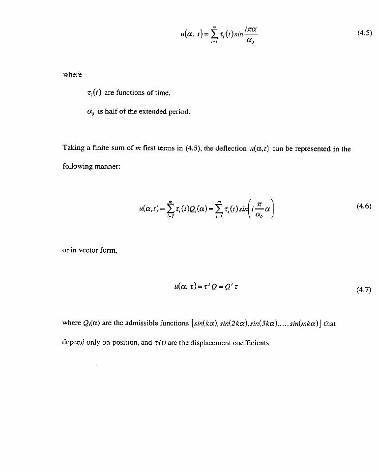
where

7, ( t ) are functions of time,

a. is half of the extended period.

Taking a finite sum of m first terms in (4.5). the deflection u(a,t) can be represented in the

following rnanner:

or in vector forrn,

where Qi(a) are the admissible functions [s in(ka) , sin(2ka), sin(3ka), . . . , sin(mka)] that

depend only on position, and q(t) are the displacement coefficients

JL k -- - , and m is the highest mode of natural vibration. a0

Equation (4.6) represents the shape up to the i-th mode of natural, radial vibrations of

a circular arc of angle a, with both ends free. This equation will be used to discretize the

deflection function u, and thus the equations of motion obtained for a curled, flexible fibre in

a shear flow. The equations of Chapter 3 contain terms with the infinitesimal displacements

624 and 6u" . These terms, in the format of equation (4.6), can be found in the following

manner:

6u = eT& + T ~ ~ Q

but since oniy lateral vibrations are of concern, 6QT = 0, and

6u = Q'&

also,

where Q(a) and q t ) are colurnn vectors.

Chapter 5

Kinematic Inertialess Equations

With the deflection function being discretized in Chapter 4 by (4.7), and the

infinitesimal virtual displacements being given by (4.9) and (4. IO), the integro-differential

equations of Chapter 3 will now result in m + 3 coupled ordinary differential equations of

the second order. For rn = 3 , this corresponds to a dynamic system in 6 - LI, with six

equations and six unknowns.

5.1 First Kinematic Approximation

The equations of motion of Chapter 3 constitute the exact integro-differential

equations of motion for an initially cuwed flexible fibre of arbitrary mass. The absolute

mass of a pulp fibre in suspension is small when compared to its translational velocity and

acceleration, and to its rotational and vibrational components, and can be neglected (i.e. set

analysis considerably.

The resulting equations of motion become:

for S.Xa :

for f i :

for 68:

for terms containing 6u:

Substituting the expressions for the forces. namely (3.3 I) , (3.32), (3.33), and (3.34),

the resulting equations become:

for :

r j[ fn (a) sin(a + 0) + f ; (a) cos(a + da + c [ F , sin(a + 8) + F , cus(cr, + O ) ] = 0 ; O i

for 68:

for t ems containing au, the equation remains unchanged as:

The expressions of the fluid forces in slow and medium flows are linear with respect

to the relative velocities of the fluid and the fibre, and are given as,

where U , and U, are the normal and tangential components of the fluid velocity, V, and V,

are the normal and tangentiai components of the fibre velocity, and k, and k, are constants

that depend on the geometry of the fibre, see (2.2) and (2.3).

As in [26], the functions k, and kt can be taken as Cox's [6] first order

approximation:

This section develops the inertialess equations which can be represented in matrix

notation. Substituting expressions (5.9) - (5.12) for the fluid forces into equations (5.5) -

(5.8), and simplifying, we have:

for :

a n

rkn 7 cos(a + 0)da - rk, y sin(a + 9 ) d a = O O

for & :

a 1 a 1

rk,, / y, sin(a + 8 ) d a + rk, 1 cm(a + 0)da =

for 6t3

a t EI- a't a t

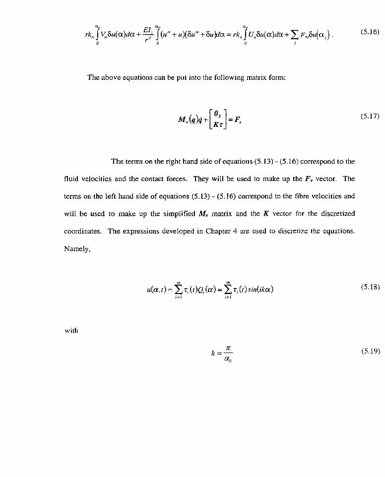
rk,, j ~ , G u ( a ) d a + -J; (u" + u)(Gu" + Su)da = rk, 1 ~ , ~ c r ( a ) d a + 2 ~,,,&(a, ) . (5.16) O O O J

The above equations can be put into the following matrix form:

The terrns on the right hmd side of equations (5.13) - (5.16) correspond to the

fluid velocities and the contact forces. They will be used to make up the F, vector. The

terms on the left hand side of equations (5.13) - (5.16) correspond to the fibre veIocities and

will be used to make up the sirnplified M, matrix and the K vector for the discretized

coordinates. The expressions developed in Chapter 4 are used to discretize the equations.

Namely,

m m

.(a, f ) = 2, ( t ) ~ , (a) = 7, ( t ) s in( ika)

with

term, can now be calculated using expression (5.18) and (5.19).

After simplification of the equations, the F, matrix for rrz modes of motion is given

as:

(5.20)

a,, a n an au

rk, c o s 8 j ~ ~ cosudn- rk,, s i n û I ~ , sinadu-rk, c o s 8 1 ~ , s inada- rk, s i n û l ~ , cosada O O O O

a n QI! 1 rk,, cos 04 Un sin &a + rk, sin 8 J Un c m aria + rk, cos 9 1 U, cos or?a - rk, sin 0 sin ado O O O

The diagonal stiffness matrix K is of size rn x rn , and after discretization is given as:

Substituting the necessary expressions for Q, and Q , ~ in the above expression for K, yields:

The vector of generalized coordinates q is given as:

Matrix Mv(q) is a (3+ m) x (3+ m) square matrix of coefficients to the fibre

velocities. The directions for the fibre velocities V. and V, are the same as those in Figure

3.2.3-1. for the forces FN and FT, and are derived by inverting (3.23):

convenience as:

Substituting equations (5.25) - (5.28) into (5.13) - (5.16), yields a system of six

equations for six unknowns and can be represented in matrix notation. Much simplification

and manipulation is required to obtain Mv in a closed analytical form. The 3 + rn rows of

the ( 3 + m ) x (3+ m ) Mv matrix are presented according to the following scheme:

Where, Row 1 is made up of:

Row 2 is made up of:

. . . ~ ( i ) l = rk,, (b, cos0 -n i sin O) .

i= l

D A2 = (rk,, - rk , )2 ,

)Il

T ( i ) Z = rk,, ( r i i cos9 + bi sin 8) . i=I

m rn I

C3 = rJk,a, , + 2 r 2 k , C c i C + rk, ç liri , i=l i = l

~ ( 3 + j ) = rk, (b, cos9 - u , sin 9 ) ,

I , is the integral inside the summation sign, and is solved by cornputer.

The expressions in the Mv matrix make use of the following constants:

1 i ( i k - 1 ) sin(ik + I ) c ~ , - ?[ (ik-1) ( ik + 1) 1

sin 2a,

sin' a, 17

The inertialess equations for rn = 3 modes of motion can be found in the appendix.

Chapter 6

Numerical Mode1

A numerical mode1 to simulate curved fibre motion implementing the kinematic

inertialess equations of Chapter 5 is developed in this chapter. A C++ code utilizing the

Runge-Kutta method is used for the simulations.

6.1 Runge-Kutta Method

The equations of the analysis, equations (5.7) and (5.8) contain the harmonic

representation of the deflection function u. These equations will be solved numerically for

the normal modes of u and stepped through the flow field. The numerical methods of

current interest are concerned with obtaining approximate sotutions for initial value

problems of the form

These approximate solutions are found at particular, discrete points of x using only the

operations of addition, subtraction, multiplication, division, and functional evaluations.

These points are: .uo, x, , x? , . . ., xn where x, - xn-, = x, - .u, = x, - xo = h ; Iz being an

arbitrary stepsize specified by the user. In general, a smaller h value yields a more accurate

approximate solution. Numerical methods are referred to as being of order n; n being zi

positive integer refening to the exactness of a particular numerical method for polynornials

of degree n or less. Thus, if the true solution to which a numerical approximation is sought

is of order n or less, the tnie solution and the approximate solution are in fact identical.

Generally, the higher the order of a particular solution, the greater the accuracy.

There are a wide variety of numerical methods currently in use to solve initial value

problems. The particular numerical method deployed depends on the problem at hand. Our

deflection function profits from a relatively simple Fourier series representation, well suited

to the classical 5'h order Runge-Kutta method with Cash-Karp constants and variable step

size.

The Runge-Kutta method is based on the Euler method which advances n solution

from x, to x,,, with a stepsize of h. The Euler method can in fact be thought of as a fïrst

order Runge-Kutta method, usually not recommended because of its low accuracy and

sets of N coupled 1" order differential equations of the form:

where the yi are functions which are derivatives of one another. The Runge-Kutta method is

self starting and combines information from several Euler-type steps to propagate a solution

over an interval. This solution is being used to match the Taylor series expansion of the

function sought up to some higher order.

The 5th order Runge-Kutta method is of the form:

k, =hf ( X , . Y , ) 3

k2 = hf (x,, + cz,h, y,, + h I k , ) ,

k, =hf ( x , +a,h,y, +b,,k,+...+b&),

y,,, = y,! + c , k , + c , k Z +c,k, +c&, +c,k, +& +0(h5) .

= y,, + c'ik, + c*lk2 + c'.fk, + c',k, + c'5k, + cB6k6 + 0 ( h 5 )

and the error estimate is

where the values for the constants ai, b, , ci , c'i , and b, are the Cash-Karp parameters, see

Press et al. [37]. The Runge-Kutta method for systern (6.2) implies for our case,

to give:

(5.29), respectively.

The algorithrn used to solve the motion of a flexibIe curved fibre in a known flow

field is defined in Section 6.2. An existing code for straight fibre flow [26] was modified

such that it applied to the curved fibre case.

6.2 Computational Algorithm

The integro-differential equations of motion of Chapter 3 contain an unknown

variable u which represents the fibre deflection. A harrnonic representation in the form of a

half-range Fourier sine series is used to discretize u, and the equations of motion are solved

via a Cc+ irnplemented Runge-Kutta routine for the generalized coordinates

6 X o , SY,, 60, and 6ti .

The numerical code used for the fibre motion simulations is a modified version of the

original 10 000 line code Lriwryshyn 1261 wrote to simulate flexible fibre motion of initial

straight fibres in a slot geometry. The modifications are necessary in order to consider an

initially curved fibre shape. The primary solution steps are:

-

Read an input file containing the fibre properties and initial positions. fluid parameters,

Runge-Kutta parameters including the desired number of steps and accuracies, time

parameters, and output files.

Set the initial Runge-Kutta conditions and fibre and fluid constants.

Cal1 the Runge-Kutta driver routine.

Update Mv, F v , and K

Solve for new fibre positions, i.e. y,,,

Estimate error using equation (6.5).

Keep the error within the desired bounds by comparing it to the vector of

desired accuracies read in (step 2). Depending on whether the error is greater

or less than the desired accuracy, reduce or increase the stepsize respectively,

and retry the step.

Save fibre shape and velocity data of current time.

Repeat steps 4 and 5 until maximum time or specified position.

The program is able to:

Test the numerical mode1 in a simple shear flow

Simulate the motion of a curved rigid or flexible fibre in complex 2-D

flows.

Simulate the motion of an essentially straight rigid or flexible fibre in

comdex 2-D flows.

Chapter 7

Model Validation and Applications

The dynamic model of the motion of curved flexible fibres will be tested for a well-

defined flow field. An essentially straight fibre case will be cornpared to analytic straight

fibre results and to prior dynamic straight fibre results of Lawryshyn and Kuhn [27]. The

model is then used to simulate the motion of a fibre in a channel and slot geometry so that

the effect of curvature on fibre passage c m be investigated.

7.1 Model Validation

To compare dynarnic curved fibre motion results to static andytic results and

dynamic straight fibre motion results, the motion and finai deflection of a straight fibre in the

flow field defined in Figure 7.1 - 1. is considered.

Figure 7.1-1. Straight fibre flow field orientation.

The straight fibre is oriented vertically in the centre of the global X-Y coordinate axis with

L a = - . Thus the fibre is symmetric with the flow field, and does not translate or rotate but

4

is only deflected by the flow field. To achieve a similar test case as that for a straight fibre,

the curved fibre is also oriented vertically and a sufficiently large radius of curvature and

correspondingly small angle are chosen.

The deflection of a stütically constrained straight beam element is, see [26]:

w here

6 is the deflection,

Fm,, is the maximum applied force,

L is the length of the beam element,

EZ is taken to be I x 10''~ ~ m ' where E is Young's modulus of elasticity and 1 is the

moment of inertia about the z axis.

Fmu is estimated from Cox's equation for the normal component of the fluid force, see (2.2),

N where Un = U,*, and V. = O, yielding a value of 9.6 x IO-' - for F,,,. The static deflection

rn

is then determined to be 0.28 mm from equation (7.1)

7.1.2 Dynamic Curved Fibre Motion

To achieve an essentially straight fibre case, a sufficiently large radius of curvature

and srnall angle is selected for the curved fibre. The product of these two values is equal to

3 mm, i.e. the analytic straight fibre length. The flow field is oriented sirnilnrly to that of

geometric parameters for the curved fibre test case in the local x--Y axis are shown in Figure

7.1.2-1.

Figure 7.1.2-1. Curved fibre orientation.

To achieve this orientation, the following values are set:

8= - d 2 ,

Ra = 3 mm,

C R a --- - sin - 4 2 2 '

the global X-Y axes as for the straight fibre case. The flow configuration for the curved fibre

with respect to the gIobal X- Y axes is shown in Figure 7.1.2-2.

Figure 7.1.2-2. Flow configuration with respect to the global X-Y axes.

As a test case, it is assumed,

Xo = -R,

7.1.3 ResuIts and Discussion

The motion of the curved fibre with radius of curvature = 85.9 mm, angle = 2' , and

three modes of motion, is shown in Figure 7.1.3-1. As shown, the fibre is initially

essentially straight at t = O rns and reaches its steady state deflection by ? = 3 ms.

Figure 7.1.3-1. Deflection of fibre for t = O to t = 3 ms, for three modes of motion.

different radius of curvature and angle combinations. As the radius of curvature increases

and the angle decreases, the curves converge to analytic straight fibre results, and to the

dynamic straight fibre case of Lawryshyn and Kuhn [27] as shown in Figure 7.1.3-2. Radius

of curvature and angle combinations below 85.9 mm and 2' respectively, were found to

overlap with the straight fibre case, i.e. there is excellent agreement between the present

results and those of Lawryshyn and Kuhn for essentially straight fibre cases.

-0- Rad = 85.9 mm; Angle = 2 deg

+ Straight Fibre Case (Lawysh yn [ 2 6 ] ) - Analytic Straight Fibre Results [26]

time (ms)

Figure 7.1.3-2. Graph of deflection vs time for fibres of 3 »lm lengths and different radii of

curvature.

and different radii of curvature. It is interesting to note that as the radius of curvature

increases, and thus the fibre length as well, it takes longer for the deflection to mach a steady

state value.

time (ms)

Figure 7.1.3-3. Graph of deflection vs tirne for an angle of 0.0078125' and different radii

of curvature.

- - - - -

curvature and different angles. As the angle and the fibre length increase, the curves take a

longer time to reach a steady state deflection.

- 0.03 125 deg

4 7.812%-3 deg

+ 5.20&-3 deg

+ 3.90625~-3 deg

time (m)

Figure 7.1.3-4. Graph of deflection vs time for a radius of curvature of 22 rn and different

angle combinations.

mm, and angle of 0.5" for r i z = 0, 1, 2, 3, and 4 modes of motion. The tïrst and second

modes are shown to overlap, as are the third and fourth modes. Although one mode of

motion is sufficient to accurately represent the curved fibre for the simple flow field of

Figure 7.1.2-2., it is anticipated that three modes of motion will be needed for more cornplex

cases.

O 0.5 1 1.5 2 2.5 3

time (m)

Figure 7.1.3-5. Graph of deflection vs time for rn = 0, 1,2 ,3 ,4 modes of motion.

A fibre's motion into a channel with a slot serves as a simpIified mode1 of fibre

screening, and is an important application of this research. Several simulations involving the

motion of an initially curved fibre in a channel and slot geometry are run and compared with

the results of Lawryshyn [26] . (The flow field used is shown in Figure 7.2-1. with a slot to

channel velocity of 0.67, i.e. U,r /U, = 0.67 .)

Figure 7.2-1. Strearnline and velocity vector plots of flow field. U, /U,, = 0.67. (Plots

taken from Lawryshyn [26]).

The initial fibre position is shown in Figure 7.2.1-1. The midpoint of the fibre is

located 10.25 mm from the slot centerline, and the values Hfand HEL correspond to the fibre

starting height and the height of the exit layer, respectively. For a fibre to enter the slot, it's

initial position must be below the exit Iayer HEL. Each fibre possesses a specific Hf value

above which dot entry is impossible. This value, called Hf.-r determines fibre passage.

Fibres initiated into the channel at or below their respective HfcNt values enter the dot, but

übove the HI;.,, value do not.

Not to Scale

Figure 7.2.1-1. Initial Fibre Position.

A Streamline of Exit Layer

A ~ i b r e A !

The HI,,, value was determined by a process of trial and error. Simulations were run for

various Hf values until the leading edge of the fibre contacted either the downstream slot

wall, the downstream channel wall, or the dot and channel corner. Contact with the slot

wall ensured slot entry whereas contact with the channel wall held a high probability of non-

Hf Channel ; v V ! !

i

1 !< ! 1 0. 25mm

O.5Omm

! \ ! /!

! t Slot

< 1

I 3 I

lower bound for was determined as the maximum Hf value for which the leading edge

of the fibre contacted the slot wall. The values for the fibre parameters used and their Hf;.rit

values are depicted below.

1. nylon: a = 30'. R = 5.730, EI = 329 x IO-" ~m'; H,, = 0.36

2. kraft: a = 30', R = 6.875, E I = 4.4~10-" ~ m ' ; Hf,, = 0.39

Figures 7.2.1-2 and 7.2.1-3 are typical plots of fibre trajectories used to determine the Hfint

vaiues. Figure 7.2.1-2. shows a kraft fibre entering the slot at its Hf,,, value, while Figure

7.2.1-3. depicts a nylon fibre missing the slot at a value higher than its HfCNf value.

Figure 7.2.1-2. kraft: a = 30°, R = 6.875, EI = 4.4 x 10-" Mn' ; Hf ,,, = 0.39

Figure 7.2.1-3. nylon: a = 30', R = 5.730, El = 329 x 10-" ~ m ' ; Hf,,, = 0.45

7.2.2 Discussion of Results

Lawryshyn [26] proved that for straight fibres, short or flexible ones have higher Hf

values than longer or stiffer fibres. The simulations run in this chapter investigate the effect

of fibre curvature on Hf values. In each of the two cases tested, curvature played a

significant role in determining whether or not the fibre entered the slot. Below are shown

H&,, values for both the straight fibre and curved fibre case of two different fibre types.

Straight fibre parameters:

1. nylon: L = 3mm, EI = 329 x IO-" Nm2; H,,, = 0.20

2. kraft: L = 3.6mm, EI = 4.4~10- l2 Nm2; Hf,, = 0.29

1. nylon: a = 30". R = 5.730, EI = 329 x IO-" ~ n z ' ; Hf,, = 0.36

2. kraft: a = 30°, R = 6.875, EI = 4.4 x 1 O-" ~ m ' ; H,,, = 0.39

In both cases, the 30" fibre curvature served to substantiaily increase the fibre's H f c N f value

from that of a sirnilar fibre with no curvature. Thus, curved fibres tend to have higher HJ

values than their stiff counterparts, allowing for significantly more curved fibres to enter the

slot.

7.2.3 Application to Pulp Screening

Pulp screening is concerned with the fractionation of pulp fibres based on their

length or flexibility. Fibre fractionation based on flexibility is of great importance, since

flexible fibres are believed to produce better quality paper. A numerical model to simuiate

the motion of pulp fibres is beneficial to investigate the advantages of a proposed screen

geometry. Presently, no numerical models of initially curved flexible fibres exist. This

research presents a numerical model able to simulate the motion of initially curved flexible

fibres and applies it to a channel and slot geornetry which serves as a simplified screen

model. The effect of curvature on fibre passage has proved to be significant when compared

to sirnilar initially straight fibres. A greater proportion of curved fibres enter the dot than

their straight counterparts.

Chapter 8

Concluding Remarks

8.1 Summary of Numerical Mode1

Elastic fibres are believed to produce better quality paper of superior strength,

printability, and optical properties than stiff fibres. Thus, fibre flexibility is of great interest

to the Pulp and Paper industry. Although much experimental work has been done on

straight fibre motion, very little has been attempted on initially curved fibres. Numerical

research, specifically that of Lawryshyn and Kuhn [27], has modeled the motion of an

initially straight flexible fibre; no numerical modeling of curved fibre motion has been

found in the literature. This research expands upon the previous work of Lawryshyn and

Kuhn to mode1 the motion of an initially cuwed flexible fibre in a shear flow.

The curved flexible fibre is modeled as a circula arc. A set of generalized

coordinates define the absolute motion of any point dong the fibre. Becausc of the

complexity of Our force analysis, Hamilton's Principle is used to formulate the equations of

deveioped and used as the entries to Hamilton's Principle. The equations thus derived

represent the movement and deflection of every point on the fibre.

The mathematical model derived with Hamilton's Principle contains an unknown

deflection variable as a generalized coordinate. To solve for the deflection variable, it is

discretized using the Rayleigh-Ritz assurned modes method. This method discretizes the

function, not the flexible cylinder and is shown to yield faster convergence [54]. By the

method of separation of variables, the deflection function can be represented by a half-range

Fourier Sine Series with time dependent coordinates. Following the sarne approximation as

in past numerical work [26], al1 inertia or mass terms in our equations are set to zero and a

first kinematic approximation is obtained for our equations. These kinematic inertiaiess

equations are written in matrix notation and, since a11 initial boundary conditions are known,

are solved using a Runge-Kutta method implemented in a CU code. The output files of the

code plot and calculate the fibre deflection.

The numerical model for curved fibre motion has been vaIidated by comparing it

with proven results for straight fibre motion [26]. Several simulations of fibres of a

specified length having large radii of curvature and small angles have been run and

compared to a straight fibre of similar length. As the radii increases and the length

decreases, the results show very good convergence to the straight fibre case.

This research can be applied to fibre passage through different vessels , as well as

other measurement and processing techniques. The mode1 has been applied to approximate

the flow of a fibre in a channel and slot geometry; an application important to the study of

pulp screening and fractionation. Several simulations have been run for two different fibres

having a radius of curvature of 30' and compared to similar fibres of a straight

configuration. It was found that fibre curvature significantly affected fibre passage values.

The curved fibres had Idfc,,, values in the range of 35% to 80% greater than their straight

fibre counterparts. The higher the Hkn, value, the greater the number of fibres capable of

entering the slot. Thus, curved fibres have been shown to have a higher rate of slot entry

than straight fibres.

8.3 Suggested Future Work

In this research, a mode1 for the motion of a cumed flexible fibre in a shear flow, as

well as general dynamic equations of motion, have been developed and validated. A first

kinematic approximation was obtained and the equations were solved using a C++

implemented Runge-Kutta code. Several simulations were run for different fibre cases to

investigate the effect of curvature on fibre passage. It would be promising to further

investigate this effect by running more detailed simulations, as well as devising a code for

the general dynarnic system of integro-differential equations with fibres having positive

masses.

in the pulp and paper industry have a kinked initial shape as shown in Figure 8.3-1; very

Iittle research on this configuration has been atternpted thus far.

Figure 8.3-1. Possible kinked fibres.

Although theoretical research on the interaction of fibre networks exists, see for

example Soszynski [44], very little work on numerical modeling of curved and kinked fibre

interaction has been found in the literature. These topics remain a possibility for future

work.

Chapter 9

References

Batchelor, G. K., "Slender-body Theory for Particles of Arbitrary Cross-section in Stokes

Flow", Journal of Fluid Mechanics, vol. 44, pt.3, pp. 419-440 (1970).

Beckmann, P. Orthogonal Polynomials for Engineers and Scientists. Golem Press,

Boulder, CO (1973)

Beer, F. P., and Johnston, E. R. Jr., Mechnnics of Materials, 2nd Edition, McGraw-Hill,

England, UK (1992).

Boresi, A. P., Schmidt, R. J., and Sidebottom, O. M., Advanced Mechanics of Materials,

John Wiley & Sons Inc., Canada (1 993).

Bronson, R., Schaum's Outline of Modem Introductory Differential Equations,

McGraw-Hill, New York (1973).

Cox, R. G., "The Motion of Long Slender Bodies in a Viscous Fluid, Part 1. General

Theory", Journal of Fluid Mechanics, vol. 44, no. 4, pp. 791-810 (1970).

Cox, R. G., "The Motion of Long Slender Bodies in a Viscous Fluid, Part 2. Shear

Flow", Journal of Fluid Mechanics, vol. 45, no. 4, pp. 625-657 (197 1 ) .

Walls", Journal of Fluid Mechanics, vol. 227, pp. 1-33 (199 1).

9. Daily, J . W., and Bugliarello, G., "Basic Data for Dilute Fiber Suspensions in Uniform

Flow with Shear", Tappi Journal, vol. 44, no. 7, pp. 497-5 12, (196 1).

10. De Mestre, N. J. and Russel, W. B., "Low-Reynolds-Number Translation of a Slender

Cylinder Near a Plane Wall", Journal of Engineering Mathematics, vol. 9, no. 2, pp. 81-

9 1 (1975).

11. Deitel, H. M. and Deitel, P. J. C: How to Program, Englewood Cliffs, NJ (1994).

12. Forgacs, O. L. and Mason, S. G., "Particle Motions in Sheared Suspension: X. Orbits of

Flexible Threadlike Particles", Journal of Colloid Science, vol. 14, pp. 473-491 (1959).

13. Fox, R. W. and McDonald, A. T. Introduction to Fluid Mechanics. Wiley, New York

(1985).

14. Ganani, E., and Powell, R. L., "Suspensions of Rodlike Particles: Literature Review and

Data Correlations", Journal of Composite Materials, vol. 19, pp. 194-2 15, (1 985).

15. Gooding, R. W. The Passage of Fibres Through Slots in Pulp Screening. M. A. Sc.

Thesis, University of British Columbia, Vancouver ( 1977).

16. Gooding, R. W. and Kerekes, R. J., "The Motion of Fibres Near a Screen Slot", Journal

of Pulp & Paper Science, vol. 15, no. 2, pp. 59-62 (1989).

17. Gooding, R. W. and Kerekes, R. J., "Consistency Changes Caused by Pulp Screening",

Tappi Journal, vol. 75, no. 1 1, pp. 109- 1 18 (1992).

18. Greenberg, M. D. Advnnced Engineering Matlzernatics, Prentice Hall, Englewood Cliffs

NJ (1988).

Materials. Wiley, New York, NY (1 985).

20. Hu, H. H., Joseph, D. D. and Crochet, M. J., "Direct Simulation of Fluid Particle

Motions", Theoretical and Computational Fluid Dynamics, vol 3, no. 5 , pp. 285-306

( 1992).

21. Jacquelin, G., "Study of the Properties of Fibrous Networks in Suspension. Tendency of

Fibres to Agglomerate. Applications.", translated from: Tech. Rech. Paper. no. 7, pp.

22-36 (1966).

22. Khayat, R. E. and Cox, R. G., "Inertia Effects on the Motion of Long Slender Bodies",

Journal of Fluid Mechanics, vol. 209, pp. 435-462 (1989).

23. Kuhn, D. C . S., Lu, X., Olson, J. A. and Robertson, A. G., "A Dynarnic Wet Fibre

Flexibility Measurement Device", JPPS, vol. 2 1, no. 10, pp. 5337-5342 October ( 1995)

24. Kuhn, D. C. S., Oosthuizen, P. H. and Whiting, P., "A Single Slot Screen for Flexibility

Measurements", Preprints 76th Ann. Mtg., Tech. Sect., CPPA, vol. 77B, 275-280 (1990).

25. Kurnar, A. Passage of Fibres Through Screen Apertures. Ph. D. Thesis, University of

British Columbia, Vancouver (1991).

26. Lawryshyn, Y. A. Statics and Dynamics of Pulp Fibres. Ph. D. Thesis, University of

Toronto, Toronto ( 1 996).

27. Lawryshyn, Y. A. and Kuhn, D. C. S. "Numerical Modeling of the Flow of a Flexible

Cylinder", Proceedings of CFD' 95, Banff, Alberta, June, 1995.

28. Mason, S. G., "The Motion of Fibres in Flowing Liquids", Pulp and Paper Magazine of

Canada, vol 5 1, no. 10, pp. 93- 100 ( 1950).

Mass. ( 1990).

30. Meirovitch, L. Dynarnics and Control of Structures. Wiley, New York, NY (1990).

3 1. Meriam, J, L. and Kraige, L. G. Engineering Mechanics. Volume 1. Statics. John

Wiley & Sons, Inc., Canada ( 1987).

32. Meriarn, J, L. and Kraige, L. G. Engineering Medzanics. Volume 2. Dynarnics. John

Wiley & Sons, Inc., Canada (1987).

33. Milne-Thomson, L.M. Theoretical Hydrodynamics London Macmillan ( 1960).

34. Olson, J. A. The Effect of Fibre Length on Passage Through Nnrrow Apertures. Ph. D.

Thesis, University of British Columbia, Vancouver (1996).

35. Page, D. H., Seth, R. S., Jordan, B. D., and Barbe, M. C. , "Curl, Crimps, Kinks and

Mocrocompressions in Pulp Fibres - Their Origin, Measurement and Significance",

Papemaking Raw Materials, Transactions of the Eighth Fundamental Research

Symposium Held at Oxford, vol. 1, pp. 183-227 (1985).

36. Powell, R. L., "Rheology of Suspensions of Rodlike Particles", Journal of Statistical

Physics, vol. 62, nos. 5/6, pp. 1073- 1094 (199 1).

37. Press, W. H., Teukolsky, S. A., Vetteriing, W. T., and Flannery, B. P. Numerical

Recipes in C. Cambridge, Cambridge University Press, UK ( 1992).

38. Rao, S. S. Mechanical Vibrations. Addison-Wesley, Reading, M A . (1986).

39. Riese, J. W., Spiegelberg, H. L. and Kellenberger, S. R., "Mechanism of Screening:

Dilute Suspensions of Stiff Fibres at Normal Incidence", Tappi Journal, vol. 52, no. 5,

pp. 895-903 ( 1969).

Flexibility", Pulp and Paper Magazine Canada, vol. 62, no. 1, pp. T3-Tl0 ( 196 1).

4 1. Schildt, H. Teach Yourself C+ +. Osborne McGraw-Hill, Berkeley, CA ( 1992).

42. Shallhorn, P. M. and Kamis, A., "A Rapid Method for Measuring Wet Fibre Flexibility",

Trans. Tech. Sect., CPPA vol. 7, no. 4, pp. 69-74 (1981).

43. Shigley, J. E., and Mischke, C. R. Mechanical Engineering Design, McGraw-Hill,

( 1989).

44. Soszynski, R. M. "Simulation of Two-dimensionai Random Fibre Networks", Nordic

Pulp and Paper Research Journal, vol. 7, no. 3, pp. 160- 162, (1992).

45. Soszynski, R. M., and Kerekes, R. J., "Elastic Interlocking of Nylon Fibres Suspended in

Liquid. Part 1. Nature of Cohesion Among Fibres.", Nordic Pulp and Paper Research

Journal, vol. 3, no. 4, pp. 172- 179 (1988).

46. Soszynski, R. M., and Kerekes, R. J., "Elastic Interlocking of Nylon Fibres Suspended in

Liquid. Part 2. Process of Interlocking.", Nordic Pulp and Paper Research Journal, vol.

3, no. 4, pp. 180-184 (1988).

47. Spiegel, M. R. Mathematical Handbook of Fomrulas and Tables, Schaum's Outline

Series. McGraw-Hill Book Company ( 1968).

48. Stewart, J. Single Variable Calculus, Brooks/Cole, Pacific Groves CA ( 1987).

49. Stewart, J. Multivariable Culculus, Brooks/Cole, Pacific Groves CA (1989).

50. Tarn Doo, P. A. and Kerekes, R. J., "A Method to Measure Wet Fibre Flexibility",

Tappi, vol. 64, no. 3, pp. 113-1 16 (1981).

5 1. Tarn Doo, P. A. and Kerekes, R. J., "The Flexibility of Wet Pulp Fibres", Pulp and Paper

Canada vol. 83, no. 2, pp. 46-50 (1982).

NJ (1988).

53. Tirnoshenko S. P., Vibration Problerns in Engineering. Van Nostrand, New York NY

(1961).

54. Weaver, Jr., Timoshenko, S. P., and Young, D. H. Vibration Problerns in Engineering.

WiIey, New York, NY (1990).

Appendix

Inertialess Equations for m = 3 Modes of Motion

For m = 3 modes of motion, the inertialess Mv matrix is 6 x 6 and the

following discretized deflection function applies:

3 3

u(a . t ) = 7, ( t ) ~ , (a) = 7, ( t ) sinika

with

sin 3 k a

ri ( t ) =

9

The F, matrix for m=3 modes of motion is given as:

an an a, a11

rkn cos 0 Un cos orda - rk, sin 8 1 Un sin a d a - rk, cos 0 J U, sin nada - rk, sin 0 1 Ur cos adct

%I a n an *O

rk,, c o s O J ~ , , s i n a d a + r k , , s i n û J ~ , , cosada+rkr c o s û l ~ , c o s a d c r - r k , s i n e j ~ ~ s inada O O O O

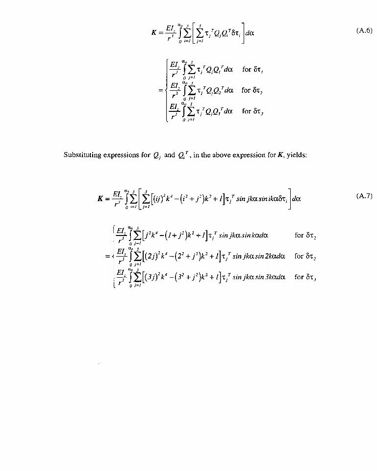
Substituting expressions for Q, and in the above expression for K, yields:

EI, a" - j x [ j 2 k 4 - ( I + j . ')k2 + i ] ~ , ' s i n jkas inkadc l for 62, r3 0 j=/

EI an 3 5 E [ ( 3 j ) ' k 4 - (3? + j ' )kz + l]~,' sin j k a s i n 3kccda for 6 ~ 3 r3 * ,=/

The six rows of the 6x6 Mv matrix are presented according to the following scheme:

Here, Row 1 is:

D B l = (rk, - rk , ) - j - .

(A. 10)

(A. 1 1)

Row 2 is:

T ( ~ ) I = rk,, (b, cos0 - a , sin 8) .

~ ( 2 ) 1 = rk, (b, cos8 - a, sin O ) ,

T(3)I = rk, (b, cos8 - a, sin O ) .

D A2 = (rk, - rk,)T ,

T (1)1= rk, (a, COS 0 + 6, siil 19) ,

(A. 13)

(A. 14)

(A. 15)

(A. 16)

(A. 17)

(A. 18)

(A. 19)

Row 3 is:

m m

C3 = r3k,n, + 2r2k, c i ~ i + rk, I i ~ i , I

1, is solved by cornputer.

Row 5 is made up of:

B4 = rk, (a , COS 8 + b, sin 6) ,

rk sin 2 ka, ~ ( 1 ) 4 = 7(ao -

rk, (sinLa, sin 3kao ~ ( 2 ) 4 = - --

2

A5 = rk,(b, cos8 - a, sine),

85 = rk, (a, cos 9 + & sin 9) .

and Row 6 is:

rk sin 4 k a o 7@)5 = $!-(ao -

A6 = rk, (6, cos0 - a, sin 8) .

B6 = rk, (a , cos9 + 6, sin 8) ,

C 6 = 0 1

sin 6 ka, ~ ( 3 ) 6 = +(a, - 6k . 1

The constants (5.46) - (5.52) apply to the above equations as in Chapter 5.

L L I I l lE

LLL 11111A 1 1 1 1 1 ~

APPLIED 4 INLAGE , lnc - - - 1653 East Main Street - - a -, Rochester. NY 14609 USA -- -- - - Phone: 71 61482-0300 -- -- - - Fax: 71 61288-5989

CI 1993. Applied Image. inc.. Ali Rights R e ~ e ~ e d