A numerical method for cell dynamics: kinetic equations ... · A numerical method for cell...

A numerical method for cell dynamics: kinetic equations withdiscontinuous coefficients∗

Aymard Benjamin†‡ Clement Frederique§ Coquel Frederic¶ Postel Marie†‡

November 5, 2012

Abstract

The motivation of this work is the numerical treatment of the mitosis in biological models involvingcell dynamics. More generally we study hyperbolic PDEs with flux transmission conditions at interfacesbetween subdomains where coefficients are discontinuous. A dedicated finite volume scheme with a lim-ited high order enhancement is adapted to treat the discontinuities arising at interfaces. The validation ofthe method is done on 1D and 2D toy problems for which exact solutions are available, allowing us to do athorough convergence study. A simulation on the original biological model illustrates the full potentialitiesof the scheme.

keywords: kinetic equations, finite volumes, discontinuous coefficients, cell dynamics

1 Introduction

Our motivation is the numerical simulation of a biological model dedicated to the ovarian follicular devel-opment. We adopt the model described in Echenim et al. [9] and references therein. This multiscale modeldescribes the latest stages of the follicular development before ovulation. The cell population of each follicleis studied as a density function depending on time, and structured according to two functional space variables,age and maturity. The density functions of the interacting follicles are solutions of weakly coupled PDE-s,where the age and maturity velocities and the loss term depend on the integro-moments of the solution for allthe follicles. The moment-based integral formulation accounts in a compact way for the feedback loop involv-ing the ovarian hormones, secreted from follicular cells, and the pituitary hormone FSH (follicle-stimulatinghormone) that targets in turn the follicular cells.∗This work is part of the Inria Large Scale Initiative Action REGATE†UPMC Univ Paris 06, UMR 7598, Laboratoire Jacques-Louis Lions, F-75005, Paris, France‡CNRS, UMR 7598, Laboratoire Jacques-Louis Lions, F-75005, Paris, France§Centre de Recherche Inria Paris-Rocquencourt, Domaine de Voluceau, Rocquencourt, B.P. 105 - F-78153 Le Chesnay, France¶CNRS and CMAP, UMR 7641, Ecole Polytechnique, route de Saclay, F-91128 Palaiseau Cedex-France

1

Numerical strategy for cell dynamics 2

The model follows the development of the follicles starting from an initial stage where all cells are proliferat-ing.. As the granulosa cells progress through subsequent cell cycles their maturity increases up to a thresholdbeyond which they exit the proliferation cell cycle and enter the differentiation stage D. The control exerted byFSH on cells depend on the cell state, whether the cell be within or outside the division cycle. Moreover, cellsbecome insensitive to any external control during a part of the cycle, leading to a drift dynamics behaving aspure transport.Cell proliferation is underlaid by the process of mitosis, through which a mother cell gives birth to two daugh-ter cells. Mitosis is the endpoint of the cell cycle that consists of the 4 phases G1, S, G2 and M, and ensuresproper DNA replication and repartition between the new cells. The most common way of representing mitosisin age-structured models of cell populations is to add a gain term in the right hand side, that controls the (av-erage) doubling time in the cell population (see the renewal equations presented in Chapter 3 of [13]). This ishowever a rough description of the mitosis event since it is distributed over all cell ages. An alternative way torepresent mitosis is to consider appropriate boundary conditions coupling the dynamics of the population ofproliferating cells with another population of cells that have exited the cell cycles. Instances of correspondingmodels can be found in the context of hematopoiesis, the process by which blood cells are produced (see e.g.[1]).Here, we consider a model where one cannot get rid of discontinuity problems, since not only the mitosisevent, but also the distinction between different phases of the cell cycle are embedded in the cell populationdynamics. Due to the phase-dependent sensitivity of cells to the extracellular signals that make them progressalong the cell cycle, discontinuities on the velocities have to be dealt with in addition to the mitosis-induceddiscontinuity. More precisely, we account for both the START transition from phase G1 to S and the EXIT

transition after mitosis completion [17].

Besides the mitosis process which eventually increases the total cell mass, the follicular development modeltakes into account apoptosis, and therefore total mass loss, by a source term which is active only locally in anarrow zone delimited by a skewed gaussian law and centered on the boundary between the first phase G1 ofthe cycle and the differentiation phase. The coefficients of the cell loss term depend on the first moment of thesolution.

From the mathematical standpoint the model describes the time evolution of the density function depending onage and maturity variables. This unknown is governed by a kinetic like equation involving velocities that arefunction of integro-moments of the unknown and the age and maturity variables. Closure equations for thesevelocities are naturally discontinuous in the age and maturity variables, precisely at biological checkpointswhich correspond to the interfaces between the biological phases. These discontinuities require additionalinformation which are handled as local double initial boundary value problems (IBVP), where inner boundaryconditions are formulated to express the biological switch [17]. First order equations with discontinuouscoefficients have received considerable attention over the past decade. Several existence and uniquenessresults have been obtained assuming the conservation of the unknown [6, 8, 14]. In our present setting suchconservation property does not hold because of the mitosis process. The well posedness of the resulting PDEmodel has been successfully studied by Shang [15]. In order to tackle its numerical approximation, varioustools are at hand. The general case of transport equations with discontinuous equations was first studied ina series of work by Bouchut and James [4] using duality arguments. Another standpoint is to address thosediscontinuities in terms of a coupling problem, as pioneered by Godlewski and Raviart [10]. We will adoptthis later setting and show that it is well suited to our purpose. We will use techniques proposed in [10] andsubsequent studies [2, 5]. Here we pay special attention to the extension of these algorithms to higher order


accuracy, which up to our knowledge, have not yet been addressed.

1.1 Outline

The remaining of the paper is organized in three sections. In Section 2, we describe the problem precisely,and, for sake of simplicity, we reduce it to a linear hyperbolic PDE with piecewise constant speeds and linearsource term, in 2D and 1D. In Section 3, we present the numerical scheme. We first recall the Finite Volumescheme and then specifically deal with the transmission conditions. In section 4, we give the results of thenumerical validation performed on several 1D and 2D test cases and based on a thorough convergence study.Whenever it is possible, the exact solutions are used as references (the derivation of the analytical solutions ispostponed to the appendix). We finally present an instance of implementation of the scheme on the full modelof the follicular development.

2 Model

The present work is devoted to the numerical simulation of one single follicle whose density of cell populationis denoted by φ. This problem is part of the much broader field of coupling problems. Let Ω ⊂ Rn, I ⊂ R,T > 0, and ∪Ni=1Ωi = Ω a non overlapping collection of subsets of Ω, a general setup can be mathematicallymodeled as: find φ : [0, T ]× Ω→ I solution of

∂tφ+ div(fi(x, φ)) = Si(x, φ), on (0, T )× Ωi, ∀i = 1 . . . N,

φ(0,x) = φ0(x), on Ω,

φ(t,x) = 0, on (0, T )× ∂Ω,

ψi(φ(t,x−)) = φ(t,x+) on (0, T )× Ωi ∩ Ωi+1,

where fi : Ωi × I → Rn and Si : Ωi × I → R are smooth functions. In the last equation modelingthe transmision condition between subsets Ωi and Ωi+1 we denote by x− (respectively x+) the boundaryΩi ∩ Ωi+1 seen from Ωi (resp. Ωi+1) side . This setup covers a wide range of applications besides cellproliferation which is our current interest here and which we will detail in the next paragraph: multiphase flowin porous media[5], traffic flow with discontinuous road surface conditions, shape-from-shading problems,sedimentation in thickener-clarifier units [7]., etc, which have generated a lot of interest and mathematicalwork in recent years.From the theoretical point of view, one of the specificities of the equation we deal with lies in its quasi linearnature. The flux functions fi are of the form

fi(x, φ) = u(x, φ)φ

arising from the weak dependance of the velocity field u on the solution φ through its first moments

u(x, φ) = v(x,m(t)), with mj(t) =

∫Ωxjφ(t,x)dx.

We are furthermore definitely in the non conservative case, since the model exhibits both mitosis – whichinduces a doubling of the mass – and a locally active source term – inducing a mass loss accounting for the


apoptosis phenomenon. The transmission conditions develop discontinuities in the solution, each time the fol-licles densities cross half cycle and cycle boundaries or depart in differentiation phase. These discontinuitiesmust be carefully handled, specially with respect to the mass computation which is one of the quantities ofinterest, along with the maturity.

2.1 2D model of the follicular development

As mentioned in the introduction, in the model proposed in Echenim et al [9] to study the development ofovarian follicles, the cell granulosa density φ is a function of time, and two so called space variables, age andmaturity. The velocities are differently defined in subregions of the global age-maturity domain as depicted inFigure 1, and can be discontinuous on the interfaces between subregions.

Figure 1: Division of the spatial domain according to the cell phases for unit cycle duration Da = 1. Left :schematic view of a granulosa cell cycle. Right : (a, γ) plane. The bottom part represents the successive cellcycles, each composed of the G1 and SM phases. The top part corresponds to the differentiation phase.

The numerical specificities arising from the coupling between different follicles have been adressed in [3] andwe focus here to the case of one single follicle. The density φ satisfies the following equation:

∂φ(x, y, t)

∂t+∂(g(x, y, u(t))φ(x, y, t))

∂x+∂(h(x, y, u(t))φ(x, y, t))

∂y= −λ(x, y, U(t))φ(x, y, t) (1)

set in the computing domain Ω in the (x, y) plane,

Ω = (x, y), 0 ≤ x ≤ Nc ×Da, 0 ≤ y ≤ 1

where Nc is the number of cell cycles and Da is the duration of one cycle. The domain Ω is divided in zonesG1, SM and D, corresponding to different cell states illustrated in Figure 1 and hence different definition ofthe speeds and source terms. Phase SM in the model aggregates the three latest phases (S, G2, M) of the cell


cycleG1 = (x, y) ∈ Ω, pDa ≤ x ≤ (p+ 1/2)Da, p = 0, . . . , Nc − 1, 0 ≤ y ≤ γs,SM = (x, y) ∈ Ω, (p+ 1/2)Da ≤ x ≤ (p+ 1)Da, p = 0, . . . , Nc − 1, 0 ≤ y ≤ γs,D = (x, y) ∈ Ω, γs ≤ y.

The aging function g appearing in (1) is defined by

g(x, y, u) =

g1u+ g2 for (x, y) ∈ G11 for (x, y) ∈ SM ∪ D

(2)

where g1, g2 are real positive constants. The maturation function h is defined by

h(x, y, u) =

τh(−y2 + (c1y + c2)(1− exp(

−uu

))) for (x, y) ∈ G1 ∪ D

0 for (x, y) ∈ SM(3)

where τh, c1, c2 and u are real positive constants. The source term, that represents cell loss through apoptosis,is defined by

λ(x, y, U) =

K exp(−((y − γs)2

γ))× (1− U) for (x, y) ∈ G1 ∪ D

0 for (x, y) ∈ SM(4)

where K, γs and γ are real positive constants.The equations in the PDE system (1) are linked together through the argument u(t) appearing in the speedsg(x, y, u) and h(x, y, u) and the argument U(t) in the source term λ(x, y, U). U(t) and u(t) represent respec-tively the plasma FSH level and the locally bioavailable FSH level and depend on some maturation momentsof the densities. In the case of one single follicle they are identical.The precise definition of the required transmission conditions has been addressed in the paper by Peipei Shang([15]). For each cycle p = 1, . . . , Nc, the flux on the x-axis is continuous between the zones G1 and SM

φ(t, x+, y) = (g1u+ g2)φ(t, x−, γ), x = (p− 1/2)Da, 0 ≤ y ≤ γs. (5)

The flux is doubling on the interfaces SM-G1, which accounts for the birth of two daughter cells from onemother cell at the end of each cell cycle

(g1u+ g2)φ(t, x+, y) = 2φ(t, x−, y), x = pDa, 0 ≤ y ≤ γs. (6)

A homogeneous Dirichlet condition holds to the north of the interface SM-D

φ(t, x, γ+s ) = 0, (p− 1/2)Da ≤ x ≤ pDa. (7)

We refer the reader to [3] and the references herein for more details on the model, but nevertheless stress outthat, as mentioned in the introduction, an important feature, which is inherent to cell dynamics, is the mitosisevent ocuring at the interface between zone G and zone SM. In most transport equations dedicated to celldynamics, it is not accounted for as such but rather by a gain term distributed over the cell population [13]. In[15], the model with discontinuous coefficients was shown to have a unique weak solution, provided that thediscontinuities in the velocities were taken into account by flux continuity – at the interfaces between zone Gand zone SM – and flux doubling – at the end of each cycle. The SM zone being a transport in age directiononly, null flux at the interface with the differentiating zone D ensures the well posedness.In this paper we will therefore focus on these specific setups, first reducing them to simpler cases where thevelocities are given instead of being weakly dependent. The closed-loop case will only be introduced in thefinal simulation.


2.2 Toy models

For the problem of interest, which is the numerical treatment of the interface conditions (5), (6) and (7),we keep the denominations G1, SM and D stemming out from the biological model for the subregions butsimplify the velocities and source coefficient to piecewise constant functions. The weak non linearity arisingfrom the dependence of the speeds and source term on the moments of the solution is left out. It is thereforesufficient to consider a simplified scalar model defined for (x, y) ∈ [0, Lx]× [0, Ly], t > 0.

∂φ(x, y, t)

∂t+∂(g(x, y)φ(x, y, t))

∂x+∂(h(x, y)φ(x, y, t))

∂y= −Λ(x, y)φ(x, y, t)

φ(x, y, 0) = φ0(x, y) (initial condition)ψL(g(x−s , y)φ(x−s , y, t)) = g(x+

s , y)φ(x+s , y, t) (flux condition on a vertical edge)

ψB(h(x, y−s )φ(x, y−s , t)) = h(x, y+s )φ(x, y+

s , t) (flux condition on an horizontal edge)

(8)

with the piecewise constant velocities g(x, y) and h(x, y) and source term Λ(x, y) defined in the subregionsdepicted on Figure 1. Furthermore, thanks to the simplicity of the geometry, we can use a cartesian griddiscretization and a numerical scheme deduced from the 1D problem by tensorization. We will thereforedescribe the numerical method on the following 1D toy problem

∂tφ(x, t) + ∂xg(x)φ(x, t) = −Λ(x)φ(x, t) for x ∈ [0, Lx], t > 0

φ(x, 0) = φ0(x) (initial condition)ψL(g(x−s )φ(x−s , t)) = g(x+

s )φ(x+s , t) (flux condition)

(9)

with

g(x) =

gL, for x < xs,gR elsewhere,

Λ(x) =

ΛL, for x < xs,ΛR elsewhere.

(10)

In order to deal with all the situations (5), (6) and (7) encountered in the real-life problem defined by equations(1) to (7), the transmission conditions in (9) will be in turn

ψL(z) = z (flux continuity between G1 and SM) (11)

ψL(z) = 2z (mitosis between SM and G1) (12)

ψL(z) = 0 (waterproof interface between SM and D) (13)

and the source term will be in turn

ΛL(x) = ΛR = 0 (No source) (14)

ΛL(x) = 1,ΛR = 0 (G1-SM) (15)

ΛL(x) = 0,ΛR = 1 (SM-G1) (16)

3 Numerical scheme

We now turn to the numerical method. We first recall the finite volume scheme in the continuous regions, andthen present the method that we have designed to deal with the transmission conditions.


3.1 Discretization

In this paragraph we describe the numerical scheme for the simplified problems (9) and (8). We refer thereader to [3] for the discretization of the full biological model (1). To solve (8 ) we set the domain dimensionsas Lx = Ly = 1. We denote by Nx the number of grid cells in each direction and by ∆x = Lx/Nx the spacestep. The step needs to be chosen so that the locations of the interfaces xs and ys, where the speed coefficientsg(x, y) and h(x, y) are discontinuous, fall on grid points. From now on we focus on the 1D finite volumescheme to solve (9), since the 2D scheme can be obtained by tensorization. Along the spatial grid

xk = k∆x, xk+1/2 = (k + 1/2)∆x, for k = 0, . . . , Nx, (17)

the time discretization is defined by

t0 = 0, tn+1 = tn + ∆tn, for n = 0, . . . , Nt (18)

with Nt such that tNt = tfinal, and time steps ∆tn that may change at each iteration, in order to preservestability. The unknowns are the approximate mean values of the solution in each grid mesh

φnk ≈1

∆x

∫ xk+1

xk

φ(x, tn)dx. for k = 0, ..., Nx − 1.

Equation (9) is then explicitly discretized to obtain a recursion formula

φn+1k = φnk −

∆tn

∆x(Fk+1(φn)− Fk(φn))−∆tnΛ(xk+ 1

2)φnk (19)

where Fk is the numerical flux across xk, designed using a limiter strategy. Indeed, it is well known that firstorder schemes, like the Godunov scheme, are diffusive, and that second order schemes, like Lax Wendroffscheme, generate oscillations in the neighborhood of discontinuities. In order to get a stable as well as precisescheme, we take a weighting of a low order scheme and a high order scheme, and we define the limitednumerical flux

Fk = FLowk + `(rk)(FHigh

k − FLowk ), (20)

where ` is the limiter function designed by Koren [12]

`Koren(r) = max(0,min(2r,2 + r

3, 2)),

and rk is defined by

rk = R ((gk+iφk+i)i=−2,...,1; (gk+i)i=−2,...,1) (21)

R ((zk+i)i=−2,...,1; (gk+i)i=−2,...,1) =

zk−1 − zk−2

zk − zk−1if gk+i ≥ 0 ∀i = −2, . . . , 1

zk+1 − zkzk − zk−1

if gk+i ≤ 0 ∀i = −2, . . . , 1

0 otherwise,

(22)

with the notation gk = g(xk). This ratio is a good indicator of the regularity of the function (see [16]). In fact,a steep gradient or a discontinuity gives a ratio far from 1, whereas a smooth function gives a ratio close to 1.The first order flux entering equation (20) is the Godunov flux

FLowk (φn) = (gnk−1)+φnk−1 + (gnk )−φnk , (23)


and the high order flux is the Lax Wendroff one, which is of second order in space wherever the function g(x)is continuous.

FHighk (φn) =

1

2(gnk−1φ

nk−1 + gnkφ

nk), (24)

The CFL stability condition is

∆tn ≤ min

(CFL

∆x

maxk |gk|,

1

maxk |Λk+ 12|

)(25)

with CFL ≤ 12 and the notation Λk+1/2 = Λ(xk+1/2).

Choosing Koren limiter in (20) provides third order in space for the convective part of the equation in eachdomain where it is continuously defined. The source term being discretized by a center point quadrature is atmost second order in each domain. Second order in time (third order when Λ = 0) is achieved by a third orderRunge-Kutta method ([11])

F1k = Fk+1(φn)− Fk(φn) + ∆xΛk+1/2φ

nk ,

φ∗k = φnk −∆tn

∆xF1k ,

F2k = Fk+1(φ∗)− Fk(φ∗) + ∆xΛk+1/2φ

∗k,

φ∗∗k = φnk −1

4

∆tn

∆xF1k −

1

4

∆tn

∆xF2k

F3k = Fk+1(φ∗∗)− Fk(φ∗∗) + ∆xΛk+1/2φ

∗∗k ,

φn+1k = φnk −

1

6

∆tn

∆xF1k −

1

6

∆tn

∆xF2k −

2

3

∆tn

∆xF3k ,

We will now focus on the interface between two subdomains where the function g can be discontinuous,neglecting the source term for the time beeing.

3.2 Treatment of discontinuous coefficients

The domain is discretized in such a manner that the interface between two subregions where g is continuous isplaced on an edge between two grid cells. Let us consider that the interface position xs = xK at the interfacebetween cells K − 1 and K as depicted on Figure 2.

To adapt the finite volume scheme designed in the previous paragraph so that it can handle the transmissioncondition, we define for each interface at grid point xk two fluxes : the left flux FL

k and the right flux FRk

(Figure 2).

Then we rewrite equation (19) as

φn+1k = φnk −

∆nt

∆x(FR

k+1 − FLk )


L

K−1 K+1K

φ φΚ−1 Κ φφΚ−2 Κ+1

KF F

K

R

Figure 2: Left and right flux surrounding an interface.

If there is no transmission condition on the flux, we have

FLk = FR

k = Fk

defined by (20). In contrast, if there is a transmission condition such as (12) for instance, we set

FRK = ψL(FL

K). (26)

The value of the numerical fluxes defined by (23) and (24) are derived for smooth coefficients g(x) andcontinuous fluxes g(x)φ(x). They must therefore take into account the transmission condition ψL, seen fromthe left side of xs. We define, at the interface K, the first order flux

FLow,LK (φn) = (gnK−1)+φnK−1 +

1

2(1− sign(gnK))ψ−1

L (gnKφnK), (27)

and the second order flux

FHigh,LK (φn) =

1

2

(gnK−1φ

nK−1 + ψ−1

L (gnKφnK)). (28)

Furthermore, the high order enhancement using a limited combination such as (20) is affected by the presenceof an interface not only at xK but in its vicinity. Indeed, if the velocity g(x) is positive, the limiter ”sees”interface K at neighboring interfaces k = K − 1, . . . ,K + 1 through the ratio rk. The transmission condition(26) causes the ratio (21) to depart from 1 on these interfaces and consequently induces a loss of accuracy inthe numerical scheme. This can be avoided by computing the ratio rk on the continuous quantities seen fromxk. Namely, at interfaces K − 1,K,K + 1, the limiter is computed using

rK−1 = R(gK−3φK−3, gK−2φK−2, gK−1φK−1, ψ

−1L (gKφK); (gK+i)i=−3,...,0

)rK = R (ψL(gK−2φK−2), ψL(gK−1φK−1), gkφK , gK+1φK+1; (gK+i)i=−2,...,1)

rK+1 = R (ψL(gK−1φK−1), gKφK , gK+1φK+1, gK+2φK+2; (gK+i)i=−1,...,2)

instead of (21).

To fix ideas, we apply this method in cases (11) and (12) encountered in our application model.

3.2.1 First application : Flux continuity (with discontinuous speed)

In this case the transmission condition isψL = Id.


At interface K, the condition is(gφ)RK = (gφ)LK

withgK−1 6= gK .

The transmission condition (26) provides the flux from the right side of the interface

FRK = FL

K .

The scheme works well without modification, both at first and third order.

3.2.2 Second application : Doubling flux.

In this case the transmission condition (26) is

ψL(F ) = 2F.

At interface K, the condition is(gφ)RK = 2(gφ)LK ,

withgK−1 6= gK .

The flux on the left of the interface is computed using continuous values in the definitions of (23) and (24).From the left side, the continuous values are gφ for x < xK and ψL(gφ) for x > xK . Therefore we write forthe first order flux

F low,LK = (gK−1)+φK−1 +

(gK)−φK2

,

and for the second order flux

F high,LK =

gK−1φK−1 +gKφK

22

.

Concerning the limiter, it has to take the doubling condition on three cells in the vicinity of the interface. Atinterfaces K − 1,K,K + 1 the limiter (21) is computed on the continuous quantity:

rK−1 = R(gK−3φK−3, gK−2φK−2, gK−1φK−1,

gKφK2

; (gK+i)i=−3,...,0

),

rK = R (2gK−2φK−2, 2gK−1φK−1, gKφK , gK+1φK+1; (gK+i)i=−2,...,1) ,

rK+1 = R (2gK−1φK−1, gKφK , gK+1φK+1, gK+2φK+2; (gK+i)i=−1,...,2) .

The transmission condition (26) provides the flux from the right side of the interface

FRK = 2FL

K .


4 Numerical validation

In the sequel, we present several numerical simulations to substantiate the validation of our method. Two 1Dsituations are handled, one with a flux continuity (11), another one with a doubling at the interface (12), withor without a source term (14), (15), (16). We then present two 2D test cases : a shear phenomenon which isencountered in the realistic model between zones G1 and SM and zones G1 and D, and a waterproof condition(13), which is encountered between zones SM and D. Finally we perform a convergence study on the fullbiological model.

4.1 1D test cases

For this set of test cases we can compare the numerical solution at final time tN with the exact solutiondescribed in Appendix A.1 and compute the L1-norm relative error

E∆x =

∑Nxk=0 |φNk − φnk |∑Nx

k=0 |φNk |

where φNk is the mean value of the exact solution at final time on cell [xk, xk+1]. This mean value is itselfestimated with a quadrature formula – the second order central point formula. This is actually justified forthe 1D test cases where the discontinuity of the solution coincides with a grid point. In order to recover theexpected behavior the initial condition is a smooth gaussian function of total mass equal to 1 and centered onxc=0.3.

φ0(x) =1

2πσexp

(1

2

((x− cx)2

σ2

)). (29)

-10

0

10

20

30

40

50

60

70

80

0 0.2 0.4 0.6 0.8 1 1.2

x

exact

FV

initial

a) gL = 0.5 (speed up after x = 0.5)tN = 0.4

-10

0

10

20

30

40

50

60

70

80

0 0.2 0.4 0.6 0.8 1 1.2

x

exact

FV

initial

b) gL = 1 (no velocity jump)tN = 0.2

-20

0

20

40

60

80

100

120

140

160

0 0.2 0.4 0.6 0.8 1 1.2

x

exact

FV

initial

c) gL = 2 (slow down after x = 0.5)tN = 0.1

Figure 3: 1D test case 1: flux continuity condition and velocity jump at interface x = 0.5. Snapshot of thedensity φ(x, t) at initial time and when crossing the interface between zones G1 and SM (t = tN ).


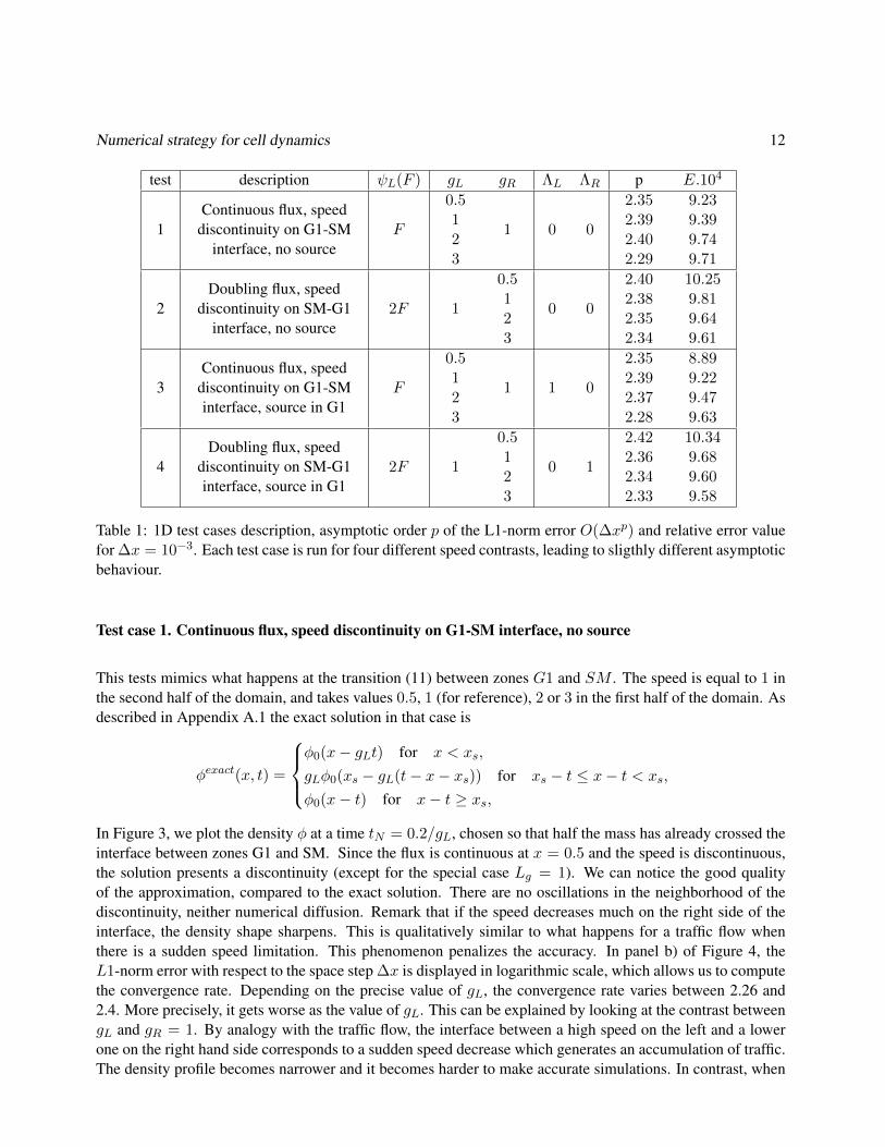
test description ψL(F ) gL gR ΛL ΛR p E.104

1Continuous flux, speed

discontinuity on G1-SMinterface, no source

F

0.5123

1 0 0

2.352.392.402.29

9.239.399.749.71

2Doubling flux, speed

discontinuity on SM-G1interface, no source

2F 1

0.5123

0 0

2.402.382.352.34

10.259.819.649.61

3Continuous flux, speed

discontinuity on G1-SMinterface, source in G1

F

0.5123

1 1 0

2.352.392.372.28

8.899.229.479.63

4Doubling flux, speed

discontinuity on SM-G1interface, source in G1

2F 1

0.5123

0 1

2.422.362.342.33

10.349.689.609.58

Table 1: 1D test cases description, asymptotic order p of the L1-norm error O(∆xp) and relative error valuefor ∆x = 10−3. Each test case is run for four different speed contrasts, leading to sligthly different asymptoticbehaviour.

Test case 1. Continuous flux, speed discontinuity on G1-SM interface, no source

This tests mimics what happens at the transition (11) between zones G1 and SM . The speed is equal to 1 inthe second half of the domain, and takes values 0.5, 1 (for reference), 2 or 3 in the first half of the domain. Asdescribed in Appendix A.1 the exact solution in that case is

φexact(x, t) =

φ0(x− gLt) for x < xs,

gLφ0(xs − gL(t− x− xs)) for xs − t ≤ x− t < xs,

φ0(x− t) for x− t ≥ xs,

In Figure 3, we plot the density φ at a time tN = 0.2/gL, chosen so that half the mass has already crossed theinterface between zones G1 and SM. Since the flux is continuous at x = 0.5 and the speed is discontinuous,the solution presents a discontinuity (except for the special case Lg = 1). We can notice the good qualityof the approximation, compared to the exact solution. There are no oscillations in the neighborhood of thediscontinuity, neither numerical diffusion. Remark that if the speed decreases much on the right side of theinterface, the density shape sharpens. This is qualitatively similar to what happens for a traffic flow whenthere is a sudden speed limitation. This phenomenon penalizes the accuracy. In panel b) of Figure 4, theL1-norm error with respect to the space step ∆x is displayed in logarithmic scale, which allows us to computethe convergence rate. Depending on the precise value of gL, the convergence rate varies between 2.26 and2.4. More precisely, it gets worse as the value of gL. This can be explained by looking at the contrast betweengL and gR = 1. By analogy with the traffic flow, the interface between a high speed on the left and a lowerone on the right hand side corresponds to a sudden speed decrease which generates an accumulation of traffic.The density profile becomes narrower and it becomes harder to make accurate simulations. In contrast, when


the speed is higher on the right, the density profile becomes smoother and it becomes easier to approximatethe solution. In any case, the best order of convergence 2.4 is achieved when gL = gR = 1. In panel a) ofFigure 4, the total mass

m0(t) =

∫[0,L]

φ(x, t)dx

is displayed with respect to the time to check whether the scheme is conservative.

0

0.5

1

1.5

2

0 0.05 0.1 0.15 0.2 0.25

mass

t

gL =0.5gL =1. gL =2. gL =3.

a) Mass with respect to time

0.0001

0.001

0.01

0.1

1

10

0.001 0.01

E1(

∆x)

∆x

gL = 0.5gL = 1gL = 2gL = 3

b) Error convergence with respect to ∆x

Figure 4: 1D test case 1: flux continuity condition and velocity jump at interface x = 0.5. In panel a) the totalmass remains constant with time. In panel b) the L1-norm error goes to 0 with ∆x. The convergence rates(around 2.4) are gathered in Table 4.1.

We also perform a 2D generalization of this test in the case gL = 2, with a smooth initial condition

φ0(x, y) =1

2πσ2exp

(1

2

((x− cx)2

σ2+

(y − cy)2

σ2

)). (30)

centered on (cx, cy) = (0.3, 0.15) and the same variance σ2 = 0.002 as before. The corresponding results aredisplayed on Figure 5.

a) Initial time. The densitybump lies in zone G1.

b) Intermediate time t = 0.15. c) Final time t = 0.25. The densitybump lies in zone SM.

Figure 5: 2D visualization of test case 1: flux continuity condition and velocity jump at interface x = 0.5,uL = 0.5, uR = 1. Snapshot of the density (initial time, passing interface, final time). (CFL = 0.4,∆x =0.001).


-50

0

50

100

150

200

250

300

350

0.6 0.8 1 1.2 1.4 1.6

x

exact

FV

initial

a) gR = 0.5

-20

0

20

40

60

80

100

120

140

160

0.6 0.8 1 1.2 1.4 1.6

x

exact

FV

initial

b) gR = 1 (no velocity jump)

0

10

20

30

40

50

60

70

80

0.6 0.8 1 1.2 1.4 1.6

x

exact

FV

initial

c) gR = 2 (no density jump)

Figure 6: 1D test case 2: doubling flux condition and velocity jump at interface x = 1. Snapshot of the densityφ(x, t) at initial time and when crossing the interface between zones G1 and SM (t = 0.2).

Test case 2. Doubling flux, speed discontinuity on SM-G1 interface, no source

The second test case mimics the mitosis (12) event occuring between the SM and G1 zone at xs = 1. Thespatial range of interest is thus shifted to [0.5, 1.7]. The initial condition is centered on xc = 0.8. The speedis equal to gL = 1 for x < xs and takes successively the values gR = 0.5,1,2 or 3 for x > xs. This time theexact solution is

φexact(x, t) =

φ0(x− t) for x < xs,2gR

(φ0(xs − t− (x−xs)gR

)) for (xs − gRt) ≤ (x− gRt) < xs,

φ0(x− gRt) for (x− gRt) ≥ xs,

In Figure 6, we plot the density φ at time t = 0.2. This corresponds to the time at which half the mass hasalready crossed the interface between zones SM and G1. The solution is continuous when gR = 2, but exhibitsa discontinuity in slope. We can draw the same conclusions as the first test case. In particular, there are nooscillations in the neighborhood of the discontinuity, even if there is a discontinuity in the solution.


0

0.5

1

1.5

2

0 0.05 0.1 0.15 0.2 0.25 0.3 0.35 0.4

mass

t

gR =0.5gR =1. gR =2. gR =3.

a) mass with respect to time

0.001

0.01

0.1

1

10

0.001 0.01

E1(

∆x)

∆x

gR = 0.5gR = 1gR = 2gR = 3

b) L1-norm error with respect to ∆x

Figure 7: 1D test case 2. Doubling flux condition and velocity jump at interface x = 1. The mass in panel a)has doubled when all the density has reached the second subdomain, as expected. In panel b) the L1-normerror goes to zero with ∆x. The convergence rates (around 2.4) are displayed in Table 4.1.

In panel b) of Figure 7 we plot in a log scale the L1-norm error with respect to the space step ∆x. Theconvergence rates, gathered in Table 4.1, are similar to the first test case, which means that the transitioncondition has not reduced the precision of the scheme. We can notice that the lower the gR, the worse theerror. This is the inverse situation to the first test case which can be explained by the same analogy withthe traffic flow. In panel a) of Figure 7 we plot the mass with respect to time. Once all the cells have beentransported in the right subdomain, the mass is doubled. As expected, since the speed is always gL = 1in the left subdomain, in all cases the densities reach the interface at the same time and the mass profilesare identical. Figure 8 displays the 2D generalization of the second test case with the initial condition (30)centered this time on (cx, cy) = (0.8, 015).

a) Initial time. The densitybump is in zone SM.

b) Intermediate time t = 0.16. c) Final time t = 0.4. The densitybump is in zone G1.

Figure 8: 2D visualization of test case 2. Doubling flux condition and velocity jump at interface x = 1uL = 1, uR = 0.5. Snapshots of the density (initial time, passing interface, final time). The mass is doubling.(CFL = 0.4,∆x = 0.001).


-10

0

10

20

30

40

50

60

70

80

0 0.2 0.4 0.6 0.8 1 1.2

x

exact

FV

initial

a) gL = 0.5, tN = 0.4

-50

0

50

100

150

200

250

0 0.2 0.4 0.6 0.8 1 1.2

x

exact

FV

initial

b) gL = 3.0, tN = 0.0666

Figure 9: 1D test case 3: flux continuity condition and velocity jump at interface x = 0.5, with source onthe left. Snapshot of the density at initial time and when crossing the interface between zones G1 and SM(t = tN ).

Test case 3. Continuous flux, speed discontinuity on G1-SM interface, linear source on the left

The third test case is the same as the first one but with a linear source term ΛL = 1 in the left part of thedomain. The exact solution, detailed in Appendix, is

φexact(x, t) =

φ0(x− gLt) exp(−t) for x < xs,

gLφ0(xs − gL(t− x− xs)) exp(−t+ x− xs) for xs − t ≤ x− t < xs,

φ0(x− t) for x− t ≥ xs,

As in the first test case, we plot the density at time tN , when half the mass has already crossed the interfacebetween zones G1 and SM. Two cases g=0.5 and gL = 3 are represented respectively on panels a) and b) ofFigure 9. The convergence study is illustrated in panel b) of Figure 10. The scheme still works well with thesource term, although the asymptotic order for the L1-norm error is 2.4, which is slightly less accurate thanwithout the source term. Since the source term is active on the left subdomain, there is a loss in mass until tehdensity bump reaches the interface (see panel a of Figure 10) In the case where gL = 3, the mass stabilizesafter the density has passed through the interface. In the case where gL = 0.5 the density bump has not entirelypassed through the interface at t = 0.25 so that the mass is not yet stabilized.cette remarque est interessantepour l’application bio: le temps de transit dans la zone ou le terme d’apoptose est actif conditionne en partiela masse finale.


Test case 4. Doubling flux, speed discontinuity on SM-G1 interface, linear source

The fourth test case is the same as the second one but with a linear source term ΛR = 1 in the right part of thedomain. The exact solution is then

φexact(x, t) =

φ0(x− t) for x < xs,

2gR

(φ0(xs − t− (x−xs)gR

))exs−xgR for (xs − gRt) ≤ (x− gRt) < xs,

φ0(x− gRt)e−t for (x− gRt) ≥ xs,

As in the second test case, we plot the density at time t = 0.2, for two values gR = 0.5 and gR = 3 respectivelyon panels a) and b) of Figure 11. Here also the asymptotic order of convergence for the error is roughly 2.4(see panel b) of Figure 12). The source term is active in the right subdomain. The mass, observed in panel a)of Figure 12, first doubles as the density bump goes through the interface, then diminishes as soon as the lossterm becomes active. The drop in mass begins at the same time in both cases gR = 0.5 and gR = 3 since theinterface is reached with the same left speed. In the biological model the final mass is indeed the result of theproliferation due to mitosis, compensated by the loss due to apoptose.

0

0.5

1

1.5

2

0 0.05 0.1 0.15 0.2 0.25

mass

t

gL =0.5gL =3.

a) L1 norm error

0.0001

0.001

0.01

0.1

1

10

0.001 0.01

E1(

∆x)

∆x

gL = 0.5gL = 1gL = 2gL = 3

b) mass with respect to time

Figure 10: 1D test case 3: flux continuity condition and velocity jump at interface x = 0.5, linear sourceon the left. In panel a) the mass decreases with time before the density has passed the interface (CFL =0.4,∆x = 0.001). In panel b) the L1-norm error goes to zero with ∆x. The convergence rates (around 2.4)are displayed in Table 4.1.


-50

0

50

100

150

200

250

300

0.6 0.8 1 1.2 1.4 1.6

x

exact

FV

initial

a) gR = 0.5

-10

0

10

20

30

40

50

60

70

80

0.6 0.8 1 1.2 1.4 1.6

x

exact

FV

initial

b) gR = 3

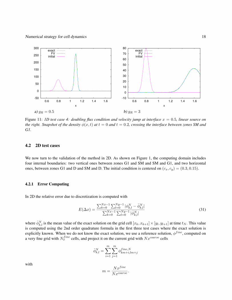
Figure 11: 1D test case 4: doubling flux condition and velocity jump at interface x = 0.5, linear source onthe right. Snapshot of the density φ(x, t) at t = 0 and t = 0.2, crossing the interface between zones SM andG1.

4.2 2D test cases

We now turn to the validation of the method in 2D. As shown on Figure 1, the computing domain includesfour internal boundaries: two vertical ones between zones G1 and SM and SM and G1, and two horizontalones, between zones G1 and D and SM and D. The initial condition is centered on (cx, cy) = (0.3, 0.15).

4.2.1 Error Computing

In 2D the relative error due to discretization is computed with

E(∆x) =

∑Nx−1k=0

∑Ny−1l=0 |φNk,l − φNk,l|∑Nx−1

k=0

∑Ny−1l=0 |φNk,l|

(31)

where φNk,l is the mean value of the exact solution on the grid cell [xk, xk+1]× [yl, yl+1] at time tN . This valueis computed using the 2nd order quadrature formula in the first three test cases where the exact solution isexplicitly known. When we do not know the exact solution, we use a reference solution, φfine, computed ona very fine grid with Nfine

x cells, and project it on the current grid with Nxcoarse cells

φNk,l =m∑i=1

m∑j=1

φfine,Nkm+i,lm+j

with

m =Nxfine

Nxcoarse.


0

0.5

1

1.5

2

0 0.05 0.1 0.15 0.2 0.25 0.3 0.35 0.4

mass

t

gR =0.5gR =3.

a) mass with respect to time

0.001

0.01

0.1

1

10

0.001 0.01

E1(

∆x)

∆x

gR = 0.5gR = 1gR = 2gR = 3

b) L1 norm error

Figure 12: 1D test case 4: doubling flux condition and velocity jump at interface x = 0.5, linear source on theright. The mass increases just after the interface, then decreases when the density has passed the interface.The convergence rates (around 2.4) are displayed in Table 4.1.

2D test case 1 : shear interface

For this test case the speed is vertical g(x, y) = 0, h(x, y) = 1 in the bottom part of the computing domain(G1∪SM). In the top part (D), the speed is oblique g(x, y) = 1 and h(x, y) = 1. The discontinuity in speedis located on the x-axis at ys = 0.3. On the snapshots in Figure 13, we can observe a shear phenomenon thatcould not occur in 1D. We also notice that the change of direction of the speed transforms the shape of thedensity bump, from circular to elliptic. The total mass remains constant. Due to the shear, the asymptotic rateof convergence of the error drops to 2.1 (see panel a) of Figure 14) .

4.2.2 2D test case 2: waterproof interface

In this test case, the speed is diagonal g(x, y) = 1, h(x, y) = 1 in zone G1 ∪D, and horizontal g(x, y) = 1,h(x, y) = 0 in zone SM . On the snapshots in Figure 15, we can observe a phenomenon of waterproofinterface that could not occur in 1D. The fraction of the mass which crosses the vertical interface betweenzones G1 and SM remains trapped in zone SM and can only move horizontally. The convergence rate dropsto 1 (panel b) of Figure 14).


a) Initial time. The densitybump lies in zone G1.

b) Intermediate time t = 0.15. c) Final time t = 0.25. The densitybump lies in zone D.

Figure 13: First 2D test case, shear phenomenon. Snapshot of the density (initial time, passing interface, finaltime). (CFL = 0.4,∆x = 0.001).

a) First order approximation. b) Third order approximation. c) Exact solution.

Figure 15: 2D test case 2 : waterproof interface. Density at final time (First and third order computationsand exact solution). Some numerical diffusion affects the shape of the density, due to the splitting of the initialdensity bump into two separate clouds.

In order to understand better the drop in precision for the 2D test case 2, we have studied other values forh(x, y) = hB in the zone SM, ranging from the reference case with no speed variation (hB = 1) and thewaterproof test case (hB = 0). Figure 16 displays the density at time t = 0.25 for three different hB values.For hB = 0.9, the solution displayed on panel a) looks very much like that obtained with the reference case.For hB = 0.001, the solution displayed in panel c) looks very much like that obtained with the waterproofboundary in Figure 15.


0.001

0.01

0.1

1

0.001 0.01

E1(

∆x)

∆x

E

∆x2.24

a) 2D test case 1 : shear.

0.01

0.1

1

0.001 0.01

E1(

∆x)

∆x

E

∆x1.03

b) 2D test case 2 : waterproof.

Figure 14: 2D test cases. L1-norm relative error with respect to ∆x. The convergence rate is 2.24 in the shearcase (panel a) and drops to 1.03 in the waterproof case (panel b).

a) hB = 0.9 b) hB = 0.5 c) hB = 0.001

Figure 16: From constant diagonal speed to waterproof interface. Solution at time t = 0.25 for three differentvalues of the vertical speed in the SM zone a) hB = 0.9, b) hB = 0.5, c) hB = 0.001

Since the exact solution is not available except for the extreme values, hB = 0 or 1, we compute the error witha converged solution computed with ∆x = 5E − 4. The different error curves and the variation of the errororder with respect to hB are displayed respectively on panel a) and b) of Figure 17. This numerical experimentconfirms that there is a regular drop in precision as the contrast between the vertical speeds on both sides of theinterface between zones SM and D increases. It is worth noting that the asymptotic order for the waterproofcase (hB = 0) computed using the converged solution is 1.25 instead of the value 1 obtained when using theexact solution in formula (31). On the other hand, the asymptotic order for the reference case with constantdiagonal speed (hB = 1) is 2.25, which is less than the asymptotic order 2.4 obtained in the 1D test case 1for gL = gR = 1. This small drop in precision is generally encountered with 2D schemes on cartesian gridsobtained by tensorization of a 1D scheme.


0.0001

0.001

0.01

0.1

1

0.001 0.01

E1(

∆x)

∆x

1.0

0.9

0.8

0.7

0.6

0.5

0.1

0.

a) Relative error variation.

1.2

1.4

1.6

1.8

2

2.2

2.4

0 0.2 0.4 0.6 0.8 1

p

hB

p

b) Order p as function of hB .

Figure 17: From constant diagonal speed to waterproof interface. a) Relative error and best least-square fitO(∆xp) for different constant hB values of the vertical speed in zone SM. b) Asymptotic order p as a functionof hB value in zone SM.

Simulation of the biological model

Our latest test performs the convergence study on the full model for the follicular development presented inthe paragraph 2.1. However we restrict ourselves to only one follicleNf = 1, and we stop the simulation aftera duration tN = 1, short enough so that the computations on very fine grids remain tractable.


t=0 initial condition t=0.02 horizontal speed discontinuity

t=0.13 horizontal speed discontinuity and mitosis t=0.17 differentiation in upper domain

t=0.18 second horizontal speed discontinuity t=0.22 waterproof boundary

Figure 18: Third 2D test case : snapshots of the density at different times of the follicular development,∆x = 0.0125. The color code is time related. Blue and red colors indicate respectively null and maximumdensity

The weak non linearity is modeled through the dependance of the speeds and FSH level on the first moment ofthe density. When dealing with only one follicle, the follicular m(f, t) and ovarian M(t) maturities are equal

M(t) = m(1, t) =

∫ 1

0

∫ NcDa

0γφ1(a, γ, t)dadγ. (32)

The plasma FSH level U(t) showing up in the arguments of the source term in (1) is defined by

U(t) = Umin +1− Umin

1 + exp(c(M(t)− M)), (33)

where Umin, c and M are real positive constants.The locally bioavailable FSH level u1(t) showing up in the arguments of the speeds in (1) is defined by

u1(t) = min

(b1 +

eb2m(1,t)

b3, 1

)U(t), (34)


0.001

0.01

0.1

1

10

0.001 0.01

E1(∆

x)

∆x

order 3∆x

1.87

order 1∆x

0.78

Figure 19: Third 2D test case : follicular development model. Numerical convergence rates with the ( order 1and) order 3 schemes, best least-square fit with O(∆x2).

where b1, b2 and b3 are real positive constants.The values of the parameters are gathered in Table 2. The age and maturity speeds parameters have chosenso that, with tN = 1, all of the three interesting transitions : G1-SM, SM-G1 and G1-D do happen, as wellas the waterproof phenomenon between zones SM and D. To illustrate these phenomena, snapshots of thedensity at significant times of the follicular development are displayed on Figure 18. For this simulation,a space discretization ∆x = 0.0125 (Nm = 80 cells per half cycle) is used, leading to a varying timediscretization of ∆t ≈ 0.0012 which meets condition (25) . The numerical convergence of the scheme isillustrated on Figure 19. The relative error with respect to a converged solution obtained using a very finegrid of Nm = 1920 cells per half cycle is displayed as a function of the space step ∆x. The asymptoticorder of convergence computed by least square fitting is almost 2. The biological model combines all thenumerical difficulties studied separately in the six previous test cases. As expected, the order of convergenceis intermediate between the best and worst order achieved for these toy problems.

References

[1] M. Adimy, F. Crauste, and S. Ruan. A mathematical study of the hematopoiesis process with applicationsto chronic myelogenous leukemia. SIAM Journal on Applied Mathematics, 65(4):1328–1352, 2005.


Parameter Description ValueCFL CFL condition 0.4

FSH plasma level (eq. (33))Umin minimum level 0.5c slope parameter 2.0M abscissa of the inflection point 4.5

Apoptosis source term (eq. (4))K intensity factor 0.1γ scaling factor 0.01γs cellular maturity threshold 0.3

intrafollicular FSH level (eq. (34))b1 basal level 0.08b2 exponential rate 2.25b3 scaling factor 1450.

Aging function (eq. (2))g1 rate 2.g2 origin 2.τh

Maturation function (eq. (3))

2.c1 0.68c2 0.08u 0.02

Table 2: Values of the parameters for the biological model simulation

[2] A. Ambroso, C. Chalons, F. Coquel, E. Godlewski, F. Lagoutiere, P.-A. Raviart, and N. Seguin. Relax-ation methods and coupling procedures. Internat. J. Numer. Methods Fluids, 56(8):1123–1129, 2008.

[3] B. Aymard, F. Clement, F. Coquel, and M. Postel. Numerical simulation of the selection process of theovarian follicles. http://hal.archives-ouvertes.fr/hal-00656382, Submitted.

[4] F. Bouchut and F. James. One-dimensional transport equations with discontinuous coefficients. Nonlin-ear Anal., 32(7):891–933, 1998.

[5] B. Boutin, F. Coquel, and LeFloch P. G. Coupling techniques for nonlinear hyperbolic equations. iii.well-balanced approximation of thick interfaces. arXiv:1205.2437, 2012.

[6] R. Burger and K. H. Karlsen. Conservation laws with discontinuous flux: a short introduction. J. Engrg.Math., 60(3-4):241–247, 2008.

[7] R. Burger, K. H. Karlsen, and N. H. Risebro. A relaxation scheme for continuous sedimentation in idealclarifier-thickener units. Comput. Math. Appl., 50(7):993–1009, 2005.

[8] R. Burger, K. H. Karlsen, and J. D. Towers. An Engquist-Osher-type scheme for conservation laws withdiscontinuous flux adapted to flux connections. SIAM J. Numer. Anal., 47(3):1684–1712, 2009.

[9] N. Echenim, D. Monniaux, M. Sorine, and F. Clement. Multi-scale modeling of the follicle selectionprocess in the ovary. Math. Biosci., 198(1):57–79, 2005.


[10] E. Godlewski and P.-A. Raviart. The numerical interface coupling of nonlinear hyperbolic systems ofconservation laws. I. The scalar case. Numer. Math., 97(1):81–130, 2004.

[11] S. Gottlieb and C. Shu. Total variation diminishing runge kutta schemes. Mathematics of computation,1998.

[12] B. Koren. A robust upwind discretisation method for advection, diffusion and source terms. NumericalMethods for Advection-Diffusion Problems, 1993.

[13] B. Perthame. Transport Equations in Biology. Birkhauser Verlag, Basel, 2007.

[14] N. Seguin and J. Vovelle. Analysis and approximation of a scalar conservation law with a flux functionwith discontinuous coefficients. Mathematical Models and Methods in Applied Sciences, 13(02):221–257, 2003.

[15] P. Shang. Cauchy problem for multiscale conservation laws : Applications to structured cell populations.http://arxiv.org/abs/1010.2132, 2010.

[16] P. K. Sweby. High resolution schemes using flux limiters for hyperbolic conservation laws. SIAM J.Numer. Anal., 21(5):995–1011, 1984.

[17] J. J. Tyson and B. Novak. temporal organization of cell cycle. Current Biology, 18:R759–768, 2008.

A Exact solutions

We now give the details of the exact solution computations for the 1D and 2D test cases.

A.1 Exact solutions of the 1D problem with piecewise constant speeds

Problem

∂tφ+ ∂xgφ = Λφ for [0, xs] ∪ [xs, xL]

g(x) =

gL if x < xs (discontinuous speed)gR if x ≥ xs

Λ(x) =

ΛL if x < xs (discontinuous speed)ΛR if x ≥ xs

φ(x, 0) = φ0(x) (initial condition)ψL(gLφ(x−s , t)) = gRφ(x+

s , t) (flux condition)

(35)

Case without source term We first solve this problem when ΛL = ΛR = 0, using the method of charac-teristics. The case when gR < gL is displayed in Figure 20. If there were no transmission conditions, thecharacteristics would be straight lines passing through the vertical axis. The analysis is detailed in the casewhere gL and gR speeds are positive which is the most usual situation in problems arising from biology.


x

t

Figure 20: Characteristics of a transmission problem with a transmission condition. The solution is a station-nary shock, corresponding to gR < gLψ

′L.

Solution For x < xs, considering the characteristics of∂tφ+ gL∂xφ = 0,

φ(x, 0) = φ0(x),

the solution isφ(x, t) = φ0(x− gLt) for x ≤ xs.

Using the same argument, considering the characteristics of∂tφ+ gR∂xφ = 0,

φ(x, 0) = φ0(x),

we find thatφ(x, t) = φ0(x− gRt) for (x− gRt) ≥ xs.

The solution for (x0 − gRt) < (x− gRt) ≤ xs is obtained thanks to the transmission condition

ψL(gLφ(x−s , t)) = gRφ(x+s , t), (36)

combined with the fact thatφ(x−s , t) = φ0(xs − gLt),

which leads togRφ(x+

s , t) = ψL(gLφ(x−s , t)) = ψL(gLφ0(xs − gLt)).

Defining a trace function

Tr(t) =1

gRψL(gLφ0(xs − gLt)), (37)

which acts as a boundary condition, we follow the characteristicsx(t) = gR,

x(ts) = xs,

given byx(t) = xs + (t− ts)gR,


to reach xs, at time

ts = t− (x− xs)gR

. (38)

Finally, the solution is

φ(x, t) =


T r(ts) for (xs − gRt) ≤ (x− gRt) < xs,

φ0(x− gRt) for (x− grt) ≥ xs,

where Tr is defined by condition (37) and ts is defined by (38).

Case with source term It can be deduced from the homogeneous case by changing the unknowns. In thesubregion where Λ is constant, if φ(x, t) is solution of

∂tφ+ ∂xgφ = Λφ

thenφ(x, t) = eΛtφ(x, t)

is solution of∂tφ+ ∂xgφ = 0.

We distinguish two cases :

With a source term in the left subdomain ΛL > 0 and ΛR = 0, the solution is

φ(x, t) =

φ0(x− gLt) exp(−Λt) for x < xs,

T r(ts) exp(−Λts) for (xs − gRt) ≤ (x− gRt) < xs,

φ0(x− gRt) for (x− gRt) ≥ xs.

where Tr is defined by the transmission condition (37) and ts is defined by (38).

With a source term in the right subdomain ΛL = 0 and ΛR > 0, the solution is

φ(x, t) =


T r(ts) exp(−Λ(t− ts)) for (xs − gRt) ≤ (x− gRt) < xs,

φ0(x− gRt) exp(−Λt) for (x− gRt) ≥ xs.

where Tr is defined by the transmission condition (37) and ts is defined by (38).


A.2 Exact solution of the 2D problems with piecewise constant speeds

A.2.1 Horizontal speed

Problem

∂tφ+ ∂xgφ = 0 for (x, y) ∈ [0, Lx]× [0, Ly]

g(x, y) =

gL if x < xs (discontinuous speed)gR if x ≥ xs

φ(x, y, 0) = φ0(x, y) (initial condition)ψL(φ(x−s , y, t)) = φ(x+

s , y, t) (flux condition)

(39)

Solution The solution is

φ(x, y, t) =

φ0(x− gLt, y) for x < xs,

T r(ts, y) for (xs − gRt) ≤ (x− gRt) < xs,

φ0(x− gRt, y) for (x− gRt) ≥ xs,

where Tr is defined by the transmission condition

Tr(t, y) = ψL(φ0(xs − gLt, y)). (40)

and ts is defined by (38).

A.2.2 Shear

Problem ∂tφ+ ∂yφ = 0 for(x, y) ∈ [0, Lx]× [0, ys]

∂tφ+ ∂xφ+ ∂yφ = 0 for(x, y) ∈ [0, Lx]× [ys, Ly]

φ(x, y, 0) = φ0(x, y) (initial condition)

(41)

Solution The characteristics are of the formx(t) = x0 + tD

y(t) = y0 + ts + tD

with tD the time spent in the upper zonetD = y − ys.

We can then define the solution piecewise

φ(x, y, t) =

φ0(x− tD, y − t) for (x, y) ∈ [0, Lx]× [ys, Ly]

φ0(x, y − t) for (x, y) ∈ [0, Lx]× [0, ys]


A.2.3 Waterproof

Problem ∂tφ+ ∂xφ = 0 for (x, y) ∈ [xI , Lx]× [0, ys]

∂tφ+ ∂xφ+ ∂yφ = 0 for (x, y) ∈ [0, Lx]× [0, Ly]− [xI , Lx]× [0, ys]

φ(x, y, 0) = φ0(x, y) (initial condition)

(42)

In order to close this problem, we have to add a homogeneous Dirichlet condition on the north of the limitbetween the 2 zones

φ(x, y+s , t) = 0 for x ∈ [xs, Lx]

Solution As in the precedent case the characteristics are of the formx(t) = x0 + tD,

y(t) = y0 + ts + tD.

We can then define the solution piecewise

φ(x, y, t) =

φ0(x− t, y − t) for (x, y) ∈ [0, Lx]× [ys, Ly] and(x− tD) ≤ xs0 for (x, y) ∈ [0, Lx]× [ys, Ly] and(x− tD) > xs

φ0(x− t, y − t) for (x, y) ∈ G1φ0(x− t, y − ts) for (x, y) ∈ SM

A numerical method for cell dynamics: kinetic equations ... · A numerical method for cell...

Documents

Transcript of A numerical method for cell dynamics: kinetic equations ... · A numerical method for cell...