A numerical investigation of the interplay between cohesive crackingand plasticity in polycrystalline materials

M. Paggi a,⇑, E. Lehmann b, C. Weber b, A. Carpinteri a, P. Wriggers b, M. Schaper c

a Department of Structural, Geotechnical and Building Engineering, Politecnico di Torino, Torino, Italyb Institute of Continuum Mechanics, Leibniz University of Hannover, Hannover, Germanyc Institute of Materials Science, Leibniz University of Hannover, Hannover, Germany

a r t i c l e i n f o

Article history:Received 6 March 2013Accepted 4 April 2013Available online 14 May 2013

Keywords:Cohesive zone modelCrystal plasticityIsotropic plasticityFinite element methodPolycrystalline materials

a b s t r a c t

The interplay between cohesive cracking and plasticity in polycrystals is herein investigated. A unifiedfinite element formulation with elasto-plastic elements for the grains and interface elements for the grainboundaries is proposed. This approach is suitable for the analysis of polycrystalline materials with aresponse ranging from that of brittle ceramics to that of ductile metals. Crystal plasticity theory is usedfor 3D computations, whereas isotropic VON MISES plasticity is adopted for the 2D tests on plane straincross-sections. Regarding the grain boundaries, a cohesive zone model (CZM) accounting for Mode Mixityis used for the constitutive relation of 2D and 3D interface elements. First, the analysis of the differencebetween 3D and 2D simulations is proposed. Then, considering all the nonlinearities in the model, theirinterplay is numerically investigated. It is found that the CZM nonlinearity prevails over plasticity for lowdeformation levels. Afterwards, plasticity prevails over CZM. Finally, for very large deformation, failure isruled by the CZM formulation which induces softening. The meso-scale numerical results show that thesimultaneous use of cohesive interface elements for the grain boundaries and plasticity theory for thegrains is a suitable strategy for capturing the experimental response of uniaxial tensile tests.

� 2013 Elsevier B.V. All rights reserved.

1. Introduction

The cohesive zone model (CZM) is widely applied to simulatecracking in quasi-brittle materials at the macro-scale [1–4]. Fol-lowing this approach, the heterogenous material composition is re-placed by a homogenized continuum and the resistance to crackpropagation is simulated by the action of cohesive tractions actingin the process zone. At the same time, the CZM can be used at themeso-scale to depict the phenomenon of intergranular separation[5,6], a type of failure affecting brittle ceramics with a polycrystal-line microstructure (see Fig. 1). In this modeling, the nonlinearity isconcentrated in the constitutive relation of the grain boundaries,whereas the grains are supposed to behave linear elastically.

In the majority of metals, on the other hand, large plastic defor-mation with significant elongation of the grains is observed, as,e.g., during metal forming (see Fig. 2). Even in this case, however,the load–displacement curve shows softening after the plastic re-gime, if the test is carried out up to very high displacement levels(see Fig. 3). This softening, impossible to be explained by plasticityalone, is the result of the formation of small microcracks andmicrocavities that coalescence, grow and finally lead to specimenfailure.

A range of intermediate situations is expected to exist betweenthe two aforementioned limit cases (very brittle or very ductilepolycrystalline materials). An example is the MgCa0.8 alloy hereininvestigated. This brittle magnesium alloy contains 0.8% calcium asthe only alloying element because the alloy is used for resorbableimplants. These implants degrade over a period of time and are ab-sorbed by the body. Hence they do not have to be surgically re-moved. For these applications, many conventional alloyingelements cannot be used since they are toxic to the human body.Besides the grain refinement, which is of minor importance sincethe material fully recrystallizes during extrusion, calcium increasesthe strength and reduces the tendency to corrosion. The processchain for the manufacture of the tensile specimens includes con-tinuous casting, extrusion of 30 mm diameter rods (extrusion ra-tio: 17.4; billet temperature 350 �C), machining of the specimens(up to a final thickness of 1 mm).

Though the alloying content of calcium is less than the maximalsolubility of calcium in magnesium (1.34%), degenerate eutecticsformed between the grains (see Fig. 4). These degenerate eutecticsare a result of the relatively high cooling rates during continuouscasting. This is required to reduce diffusion processes, so that thesaturated solid solution dissolves significantly less alloying ele-ments. Within the grains several elongated Mg2Ca phases wereprecipitated from the saturated solid as the solubility decreaseswith the temperature. The degenerate eutectics do not dissolve

0927-0256/$ - see front matter � 2013 Elsevier B.V. All rights reserved.http://dx.doi.org/10.1016/j.commatsci.2013.04.002

⇑ Corresponding author. Tel.: +39 011 090 4910; fax: +39 011 090 4899.E-mail address: marco.paggi@polito.it (M. Paggi).

Computational Materials Science 77 (2013) 81–92

Contents lists available at SciVerse ScienceDirect

Computational Materials Science

journal homepage: www.elsevier .com/locate /commatsci

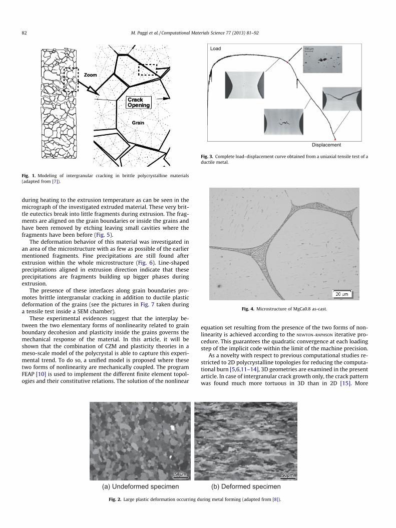
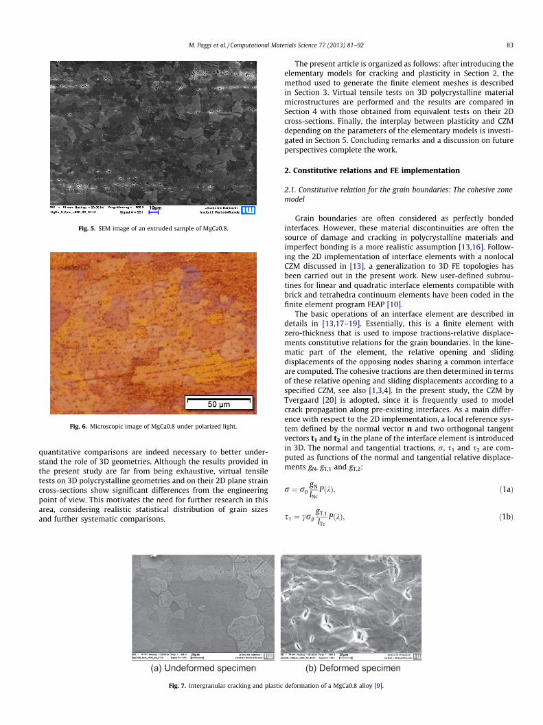
during heating to the extrusion temperature as can be seen in themicrograph of the investigated extruded material. These very brit-tle eutectics break into little fragments during extrusion. The frag-ments are aligned on the grain boundaries or inside the grains andhave been removed by etching leaving small cavities where thefragments have been before (Fig. 5).

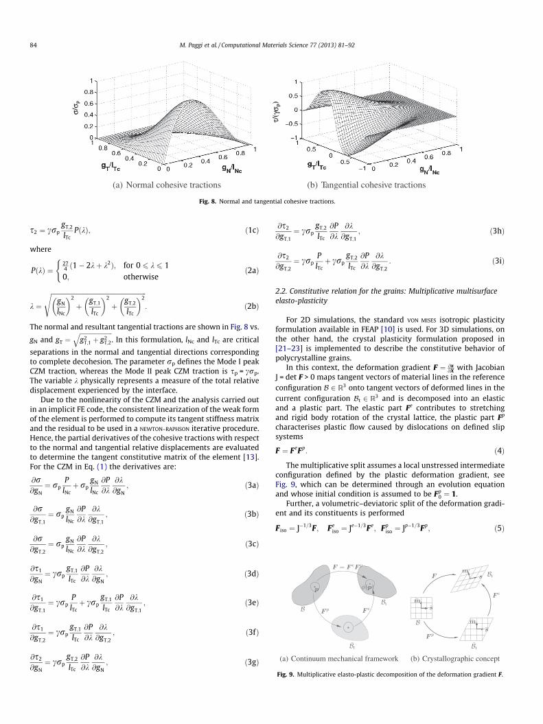
The deformation behavior of this material was investigated inan area of the microstructure with as few as possible of the earliermentioned fragments. Fine precipitations are still found afterextrusion within the whole microstructure (Fig. 6). Line-shapedprecipitations aligned in extrusion direction indicate that theseprecipitations are fragments building up bigger phases duringextrusion.

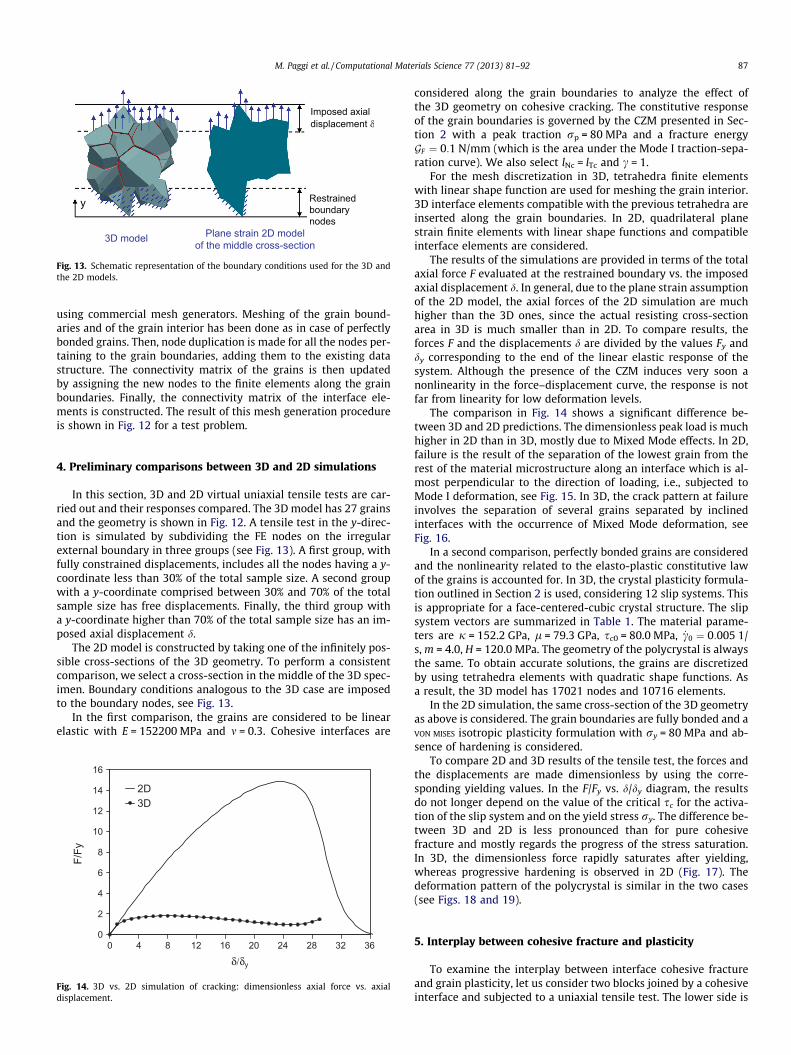
The presence of these interfaces along grain boundaries pro-motes brittle intergranular cracking in addition to ductile plasticdeformation of the grains (see the pictures in Fig. 7 taken duringa tensile test inside a SEM chamber).

These experimental evidences suggest that the interplay be-tween the two elementary forms of nonlinearity related to grainboundary decohesion and plasticity inside the grains governs themechanical response of the material. In this article, it will beshown that the combination of CZM and plasticity theories in ameso-scale model of the polycrystal is able to capture this experi-mental trend. To do so, a unified model is proposed where thesetwo forms of nonlinearity are mechanically coupled. The programFEAP [10] is used to implement the different finite element topol-ogies and their constitutive relations. The solution of the nonlinear

equation set resulting from the presence of the two forms of non-linearity is achieved according to the NEWTON–RAPHSON iterative pro-cedure. This guarantees the quadratic convergence at each loadingstep of the implicit code within the limit of the machine precision.

As a novelty with respect to previous computational studies re-stricted to 2D polycrystalline topologies for reducing the computa-tional burn [5,6,11–14], 3D geometries are examined in the presentarticle. In case of intergranular crack growth only, the crack patternwas found much more tortuous in 3D than in 2D [15]. More

Fig. 1. Modeling of intergranular cracking in brittle polycrystalline materials(adapted from [7]).

(a) Undeformed specimen (b) Deformed specimen

Fig. 2. Large plastic deformation occurring during metal forming (adapted from [8]).

Load

Displacement

Fig. 3. Complete load–displacement curve obtained from a uniaxial tensile test of aductile metal.

Fig. 4. Microstructure of MgCa0.8 as-cast.

82 M. Paggi et al. / Computational Materials Science 77 (2013) 81–92

quantitative comparisons are indeed necessary to better under-stand the role of 3D geometries. Although the results provided inthe present study are far from being exhaustive, virtual tensiletests on 3D polycrystalline geometries and on their 2D plane straincross-sections show significant differences from the engineeringpoint of view. This motivates the need for further research in thisarea, considering realistic statistical distribution of grain sizesand further systematic comparisons.

The present article is organized as follows: after introducing theelementary models for cracking and plasticity in Section 2, themethod used to generate the finite element meshes is describedin Section 3. Virtual tensile tests on 3D polycrystalline materialmicrostructures are performed and the results are compared inSection 4 with those obtained from equivalent tests on their 2Dcross-sections. Finally, the interplay between plasticity and CZMdepending on the parameters of the elementary models is investi-gated in Section 5. Concluding remarks and a discussion on futureperspectives complete the work.

2. Constitutive relations and FE implementation

2.1. Constitutive relation for the grain boundaries: The cohesive zonemodel

Grain boundaries are often considered as perfectly bondedinterfaces. However, these material discontinuities are often thesource of damage and cracking in polycrystalline materials andimperfect bonding is a more realistic assumption [13,16]. Follow-ing the 2D implementation of interface elements with a nonlocalCZM discussed in [13], a generalization to 3D FE topologies hasbeen carried out in the present work. New user-defined subrou-tines for linear and quadratic interface elements compatible withbrick and tetrahedra continuum elements have been coded in thefinite element program FEAP [10].

The basic operations of an interface element are described indetails in [13,17–19]. Essentially, this is a finite element withzero-thickness that is used to impose tractions-relative displace-ments constitutive relations for the grain boundaries. In the kine-matic part of the element, the relative opening and slidingdisplacements of the opposing nodes sharing a common interfaceare computed. The cohesive tractions are then determined in termsof these relative opening and sliding displacements according to aspecified CZM, see also [1,3,4]. In the present study, the CZM byTvergaard [20] is adopted, since it is frequently used to modelcrack propagation along pre-existing interfaces. As a main differ-ence with respect to the 2D implementation, a local reference sys-tem defined by the normal vector n and two orthogonal tangentvectors t1 and t2 in the plane of the interface element is introducedin 3D. The normal and tangential tractions, r, s1 and s2 are com-puted as functions of the normal and tangential relative displace-ments gN, gT,1 and gT,2:

r ¼ rpgN

lNcPðkÞ; ð1aÞ

s1 ¼ crpgT;1

lTcPðkÞ; ð1bÞ

Fig. 5. SEM image of an extruded sample of MgCa0.8.

Fig. 6. Microscopic image of MgCa0.8 under polarized light.

(a) Undeformed specimen (b) Deformed specimen

Fig. 7. Intergranular cracking and plastic deformation of a MgCa0.8 alloy [9].

M. Paggi et al. / Computational Materials Science 77 (2013) 81–92 83

s2 ¼ crpgT;2

lTcPðkÞ; ð1cÞ

where

PðkÞ ¼274 ð1� 2kþ k2Þ; for 0 6 k 6 10; otherwise

(ð2aÞ

k ¼

ffiffiffiffiffiffiffiffiffiffiffiffiffiffiffiffiffiffiffiffiffiffiffiffiffiffiffiffiffiffiffiffiffiffiffiffiffiffiffiffiffiffiffiffiffiffiffiffiffiffiffiffiffiffiffiffiffiffiffiffigN

lNc

� �2

þgT;1

lTc

� �2

þgT;2

lTc

� �2s

: ð2bÞ

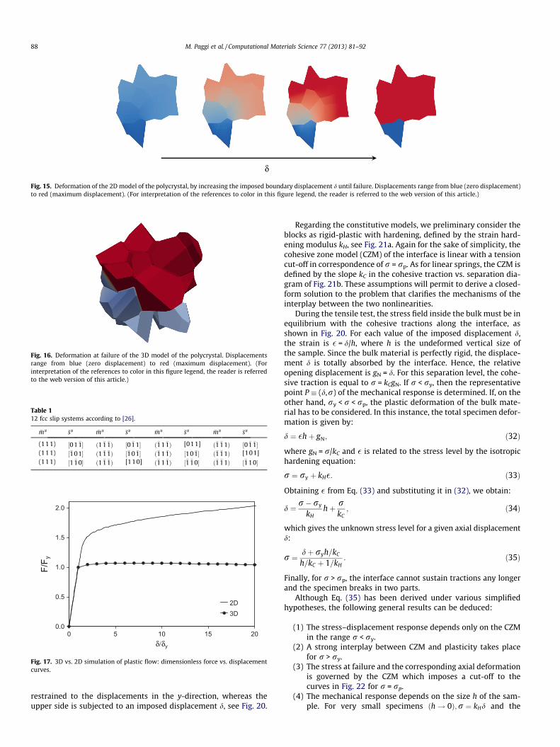
The normal and resultant tangential tractions are shown in Fig. 8 vs.

gN and gT ¼ffiffiffiffiffiffiffiffiffiffiffiffiffiffiffiffiffiffiffiffiffig2

T;1 þ g2T;2

q. In this formulation, lNc and lTc are critical

separations in the normal and tangential directions correspondingto complete decohesion. The parameter rp defines the Mode I peakCZM traction, whereas the Mode II peak CZM traction is sp = crp.The variable k physically represents a measure of the total relativedisplacement experienced by the interface.

Due to the nonlinearity of the CZM and the analysis carried outin an implicit FE code, the consistent linearization of the weak formof the element is performed to compute its tangent stiffness matrixand the residual to be used in a NEWTON–RAPHSON iterative procedure.Hence, the partial derivatives of the cohesive tractions with respectto the normal and tangential relative displacements are evaluatedto determine the tangent constitutive matrix of the element [13].For the CZM in Eq. (1) the derivatives are:

@r@gN¼ rp

PlNcþ rp

gN

lNc

@P@k

@k@gN

; ð3aÞ

@r@gT;1

¼ rpgN

lNc

@P@k

@k@gT;1

; ð3bÞ

@r@gT;2

¼ rpgN

lNc

@P@k

@k@gT;2

; ð3cÞ

@s1

@gN¼ crp

gT;1

lTc

@P@k

@k@gN

; ð3dÞ

@s1

@gT;1¼ crp

PlTcþ crp

gT;1

lTc

@P@k

@k@gT;1

; ð3eÞ

@s1

@gT;2¼ crp

gT;1

lTc

@P@k

@k@gT;2

; ð3fÞ

@s2

@gN¼ crp

gT;2

lTc

@P@k

@k@gN

; ð3gÞ

@s2

@gT;1¼ crp

gT;2

lTc

@P@k

@k@gT;1

; ð3hÞ

@s2

@gT;2¼ crp

PlTcþ crp

gT;2

lTc

@P@k

@k@gT;2

: ð3iÞ

2.2. Constitutive relation for the grains: Multiplicative multisurfaceelasto-plasticity

For 2D simulations, the standard VON MISES isotropic plasticityformulation available in FEAP [10] is used. For 3D simulations, onthe other hand, the crystal plasticity formulation proposed in[21–23] is implemented to describe the constitutive behavior ofpolycrystalline grains.

In this context, the deformation gradient F ¼ @x@X with Jacobian

J = det F > 0 maps tangent vectors of material lines in the referenceconfiguration B 2 R3 onto tangent vectors of deformed lines in thecurrent configuration Bt 2 R3 and is decomposed into an elasticand a plastic part. The elastic part Fe contributes to stretchingand rigid body rotation of the crystal lattice, the plastic part Fp

characterises plastic flow caused by dislocations on defined slipsystems

F ¼ FeFp: ð4Þ

The multiplicative split assumes a local unstressed intermediateconfiguration defined by the plastic deformation gradient, seeFig. 9, which can be determined through an evolution equationand whose initial condition is assumed to be Fp

0 ¼ 1.Further, a volumetric–deviatoric split of the deformation gradi-

ent and its constituents is performed

F iso ¼ J�1=3F; Feiso ¼ Je�1=3Fe; Fp

iso ¼ Jp�1=3Fp; ð5Þ

σσ/σ p

τ/( γ

σ p)

(a) Normal cohesive tractions (b) Tangential cohesive tractions

Fig. 8. Normal and tangential cohesive tractions.

Fig. 9. Multiplicative elasto-plastic decomposition of the deformation gradient F.

84 M. Paggi et al. / Computational Materials Science 77 (2013) 81–92

with J = Je due to fulfilling the requirement of present plastic incom-pressibility expressed through Jp = 1.

2.2.1. Thermodynamical considerationsThe deformation power per unit undeformed volume can be

written as

P : _F ¼ P : _Fe þ R : Lp; ð6Þ

where P ¼ PFpT is the 1st PIOLA–KIRCHHOFF stress tensor relative to theintermediate configuration Bt and R ¼ FeT PFpT ¼ FeTsFe�T a stressmeasure conjugate to the plastic velocity gradient Lp ¼ _FpFp�1 inBt; s being the KIRCHHOFF stress tensor on Bt. Further, it is

P ¼ FeS; S ¼ Ce�1R; Ce ¼ FeT Fe; ð7Þ

where S is the 2nd PIOLA–KIRCHHOFF stress tensor relative to the inter-mediate configuration Bt which is symmetric, Ce is further the elas-tic right CAUCHY–GREEN tensor in Bt.

The evolution of the plastic deformation gradient Fp is definedby the plastic flow equation, resulting from the plastic rate ofdeformation Lp. In the presence of nsyst systems undergoing plasticslip, represented by the plastic shear rates _ca, the plastic flow equa-tion is further generalized

Lp ¼ _FpFp�1; Lp ¼Xnsyst

a¼1

_casa � �ma; ð8Þ

�sa being the slip direction vector and �ma being the slip plane normalvector of the ath slip system f�sa; �mag. The slip system vectors havethe properties �s � �m ¼ 0 and thus ð�sa � �maÞð�sa � �maÞ ¼ 0. The gener-alization in (8) leads to the modified evolution equation of the plas-tic deformation gradient depending on the plastic slips

_Fp ¼Xa

_ca�sa � �ma

" #Fp: ð9Þ

2.2.2. The resolved SCHMID stressThe SCHMID stress sa is the projection of R onto the slip system

�sa � �ma

sa ¼ ðdev½R� � �maÞ � �sa ¼ dev½R� : �sa � �ma: ð10Þ

As the slip system tensor �sa � �ma is purely deviatoric, only thedeviator of the stress tensor contributes to the resolved stress.With the relations in (7) and some straightforward recast, it is

sa ¼ ReTsRe : �sa � �ma: ð11Þ

2.2.3. Elastic responseThe elastic part of the deformation is gained from a NEO–HOO-

KEean strain energy function. Due to assumed isotropy within theelastic contribution, the description is given in terms of the elasticleft CAUCHY–GREEN tensor be. Applying a volumetric–deviatoric splityields

qw beiso; J

e� �¼ l

2tr be

iso � 3� �

þ j2ðln JeÞ2; ð12Þ

s ¼ 2q@w

@be be ¼ l dev beiso

� �þ j ln Je 1; ð13Þ

devðsÞ ¼ l dev beiso

� �; volðsÞ ¼ j ln Je 1: ð14Þ

Because slip-system tensors are deviatoric by construction,their internal product by the hydrostatic KIRCHHOFF stress compo-nents vanishes and the SCHMID stress in (11) remains

sa ¼ l �saiso � �ma

iso; �saiso ¼ Fe

iso � �sa; �maiso ¼ Fe

iso � �ma: ð15Þ

2.2.4. A rate-dependent formulation via a viscoplastic power-lawA rate-dependent theory enables the modeling of creep in single

crystals and is performed by the introduction of a power law-typeconstitutive equation for the rates _ca of inelastic deformation inthe slip systems

_ca ¼ _c0sa

sy

jsajsy

� �m�1

¼ _c0sajsajm�1 s�my ; ð16Þ

_c0 and sy being the reference shear rate and slip resistance, and mbeing a rate-sensitivity parameter. Within an isotropic TAYLOR hard-ening model, the evolution for the slip resistance sy is considered

_sy ¼X

aH � j _caj; c ¼

Z t

0

_c dt; _c ¼X

a

_ca: ð17Þ

2.2.5. Incremental kinematicsThe slip rate is discretized with a standard backward EULER inte-

gration in order to obtain incremental evolution equations for theupdate of the evolving quantities

Dca ¼ Dt _caðFeÞ: ð18Þ

The implicit exponential integrator is then used to discretize theplastic flow Eq. (9)

Fpnþ1 ¼ exp

Xa

Dca�sa � �ma

" #� Fp

n: ð19Þ

Due to the property det½expð�sa � �maÞ� ¼ exp½trð�sa � �maÞ� ¼expð0Þ ¼ 1, it preserves the plastic volume. Here, Fe trial

nþ1 ¼ f nþ1Fen,

is the trial elastic deformation gradient with f nþ1 ¼Fnþ1F�1

n ¼ 1þ gradnðDuÞ and Jn+1 = det Fn+1, Fe trialiso ¼ J�1=3

nþ1 Fe trialnþ1 , so

that an exponential update for the new elastic deformation gradientcan be obtained

Fenþ1 ¼ Fe trial

nþ1 � expX

a� Dca�sa � �ma

" #: ð20Þ

The current trial resolved shear stress sa trialnþ1 , cf. (15), is obtained

with the current orientation of the crystal through rotation of theslip system with the trial elastic deformation gradient

sa trialnþ1 ¼ l�sa trial

iso � �ma trialiso ; �sa trial

iso ¼ Fe trialiso � �sa; �ma trial

iso

¼ Fe trialiso � �ma: ð21Þ

2.2.6. Equilibrating the plastic stateOmitting the subscript n + 1, a residual based on the exponen-

tial map is defined to equilibrate the plastic state, leading to a localNEWTON–RAPHSON algorithm through a TAYLOR expansion about thereached point Fe

k

RðFeÞ :¼ Fe � Fe trial � expX

a� Dca�sa � �ma

" #¼ 0; ð22Þ

and

Rk þ @FekRðFe

kÞ : DFek ¼ 0; ð23Þ

DFek ¼ � @Fe

kRðFe

kÞh i�1

: Rk; Fekþ1 ¼ Fe

k þ DFek; ð24Þ

with the important derivatives

@Fe RðFeÞ½ �ijkl ¼ dikdjl þ Fe trialim Emjpq

Xa

�sa � �ma � @Fe Dca

" #pqkl

; ð25Þ

M. Paggi et al. / Computational Materials Science 77 (2013) 81–92 85

Emjpq ¼@ exp �

PaDcaðFeÞ�sa � �ma

� �mj

@ �

PaDcaðFeÞ�sa � �ma

� �pq

; ð26Þ

and

@Fe Dcb ¼ Dt _c0mjsajm�1s�my ½N

ab��1@Fesa ð27Þ

@Fesa ¼ �23saFe�T þ lJ�1=3 �ma

iso � �sa þ �saiso � �ma� �

ð28Þ

Nab ¼ dab þ Dt _c0msajsajm�1s�m�1y

XbHsignðDcbÞ: ð29Þ

3. Geometrical models of the polycrystal

The polycrystal is modeled with 3D VORONOI cell shaped grains.Through the DELAUNAY triangulation of a given random point seed,a polycrystal of arbitrary size can be obtained through statingthe size of the bounding box. For the simulations based on crystalplasticity only, where the nonlinearity is solely due to the constitu-tive relation of the grain material, the grains are perfectly bondedalong their boundaries. In this case, the DELAUNAY refinement algo-rithm proposed in [24] is used for the discretization of the grainboundaries (facets). Afterwards, the DELAUNAY algorithm proposedin [25] is implemented for the FE discretization of the grain inte-rior, see the result in Fig. 10.

In order to realize randomly orientated slip systems in eachgrain of the undeformed polycrystalline structure, the slip systemvectors are rotated around the cartesian axes about three EULER an-gles U, H and W according to a y-convention, see Fig. 11 (first, arotation about the z-axis is performed, then along the y-axis and fi-nally along the new z-axis)

RW ¼cosW �sinW 0sinW cosW 0

0 0 1

264

375 RH ¼

cosH 0 sinH

0 1 0�sinH 0 cosH

264

375 RU¼

cosU �sinU 0sinU cosU 0

0 0 1

264

375

ð30Þ

R ¼ RW � RH � RU: ð31Þ

Aiming at combining crystal plasticity with cohesive zone modelsfor the simulation of grain boundary sliding and decohesion, zero-thickness interface elements have to be inserted along the grain

boundary facets. In 2D, this can be done by duplicating the nodesof the grains along the grain boundaries and constructing the con-nectivity matrix for the interface elements [13]. In 3D, this proce-dure is much more complex. The easiest way would be togenerate the polycrystalline topology using VORONOI diagrams andthen meshing each grain separately from the others. This has theadvantage that meshing can be performed by using standard geom-etry and mesh generation toolkits. However, this procedure maylead to non-matching nodes for the construction of the interfaceelements. Hence, the same procedure as in 2D is adopted, althoughit is algorithmically more complex and not possible to be performed

(a) Polycrystal consisting

of VORONOI cell grains

(b) Cut through polcrys-

talline structure

(c) Three-dimensional

view into the cuttedpolycrystal

Fig. 10. Polycrystalline model within bounding box 200 � 200 � 200 lm. The VORONOI cell shaped crystal grains are obtained through DELAUNAY triangulation of a random pointseed.

Fig. 11. Rotation of the axes around random EULER angles.

(a) Grains (b) Grain boundaries

Fig. 12. 3D grains and grain boundaries of the test problem analyzed in the sequel.

86 M. Paggi et al. / Computational Materials Science 77 (2013) 81–92

using commercial mesh generators. Meshing of the grain bound-aries and of the grain interior has been done as in case of perfectlybonded grains. Then, node duplication is made for all the nodes per-taining to the grain boundaries, adding them to the existing datastructure. The connectivity matrix of the grains is then updatedby assigning the new nodes to the finite elements along the grainboundaries. Finally, the connectivity matrix of the interface ele-ments is constructed. The result of this mesh generation procedureis shown in Fig. 12 for a test problem.

4. Preliminary comparisons between 3D and 2D simulations

In this section, 3D and 2D virtual uniaxial tensile tests are car-ried out and their responses compared. The 3D model has 27 grainsand the geometry is shown in Fig. 12. A tensile test in the y-direc-tion is simulated by subdividing the FE nodes on the irregularexternal boundary in three groups (see Fig. 13). A first group, withfully constrained displacements, includes all the nodes having a y-coordinate less than 30% of the total sample size. A second groupwith a y-coordinate comprised between 30% and 70% of the totalsample size has free displacements. Finally, the third group witha y-coordinate higher than 70% of the total sample size has an im-posed axial displacement d.

The 2D model is constructed by taking one of the infinitely pos-sible cross-sections of the 3D geometry. To perform a consistentcomparison, we select a cross-section in the middle of the 3D spec-imen. Boundary conditions analogous to the 3D case are imposedto the boundary nodes, see Fig. 13.

In the first comparison, the grains are considered to be linearelastic with E = 152200 MPa and m = 0.3. Cohesive interfaces are

considered along the grain boundaries to analyze the effect ofthe 3D geometry on cohesive cracking. The constitutive responseof the grain boundaries is governed by the CZM presented in Sec-tion 2 with a peak traction rp = 80 MPa and a fracture energyGF ¼ 0:1 N/mm (which is the area under the Mode I traction-sepa-ration curve). We also select lNc = lTc and c = 1.

For the mesh discretization in 3D, tetrahedra finite elementswith linear shape function are used for meshing the grain interior.3D interface elements compatible with the previous tetrahedra areinserted along the grain boundaries. In 2D, quadrilateral planestrain finite elements with linear shape functions and compatibleinterface elements are considered.

The results of the simulations are provided in terms of the totalaxial force F evaluated at the restrained boundary vs. the imposedaxial displacement d. In general, due to the plane strain assumptionof the 2D model, the axial forces of the 2D simulation are muchhigher than the 3D ones, since the actual resisting cross-sectionarea in 3D is much smaller than in 2D. To compare results, theforces F and the displacements d are divided by the values Fy anddy corresponding to the end of the linear elastic response of thesystem. Although the presence of the CZM induces very soon anonlinearity in the force–displacement curve, the response is notfar from linearity for low deformation levels.

The comparison in Fig. 14 shows a significant difference be-tween 3D and 2D predictions. The dimensionless peak load is muchhigher in 2D than in 3D, mostly due to Mixed Mode effects. In 2D,failure is the result of the separation of the lowest grain from therest of the material microstructure along an interface which is al-most perpendicular to the direction of loading, i.e., subjected toMode I deformation, see Fig. 15. In 3D, the crack pattern at failureinvolves the separation of several grains separated by inclinedinterfaces with the occurrence of Mixed Mode deformation, seeFig. 16.

In a second comparison, perfectly bonded grains are consideredand the nonlinearity related to the elasto-plastic constitutive lawof the grains is accounted for. In 3D, the crystal plasticity formula-tion outlined in Section 2 is used, considering 12 slip systems. Thisis appropriate for a face-centered-cubic crystal structure. The slipsystem vectors are summarized in Table 1. The material parame-ters are j = 152.2 GPa, l = 79.3 GPa, sc0 = 80.0 MPa, _c0 ¼ 0:005 1/s, m = 4.0, H = 120.0 MPa. The geometry of the polycrystal is alwaysthe same. To obtain accurate solutions, the grains are discretizedby using tetrahedra elements with quadratic shape functions. Asa result, the 3D model has 17021 nodes and 10716 elements.

In the 2D simulation, the same cross-section of the 3D geometryas above is considered. The grain boundaries are fully bonded and aVON MISES isotropic plasticity formulation with ry = 80 MPa and ab-sence of hardening is considered.

To compare 2D and 3D results of the tensile test, the forces andthe displacements are made dimensionless by using the corre-sponding yielding values. In the F/Fy vs. d/dy diagram, the resultsdo not longer depend on the value of the critical sc for the activa-tion of the slip system and on the yield stress ry. The difference be-tween 3D and 2D is less pronounced than for pure cohesivefracture and mostly regards the progress of the stress saturation.In 3D, the dimensionless force rapidly saturates after yielding,whereas progressive hardening is observed in 2D (Fig. 17). Thedeformation pattern of the polycrystal is similar in the two cases(see Figs. 18 and 19).

5. Interplay between cohesive fracture and plasticity

To examine the interplay between interface cohesive fractureand grain plasticity, let us consider two blocks joined by a cohesiveinterface and subjected to a uniaxial tensile test. The lower side is

Fig. 13. Schematic representation of the boundary conditions used for the 3D andthe 2D models.

0

2

4

6

8

10

12

14

16

0 4 8 12 16 20 24 28 32 36

δ/δy

F/Fy

2D3D

Fig. 14. 3D vs. 2D simulation of cracking: dimensionless axial force vs. axialdisplacement.

M. Paggi et al. / Computational Materials Science 77 (2013) 81–92 87

restrained to the displacements in the y-direction, whereas theupper side is subjected to an imposed displacement d, see Fig. 20.

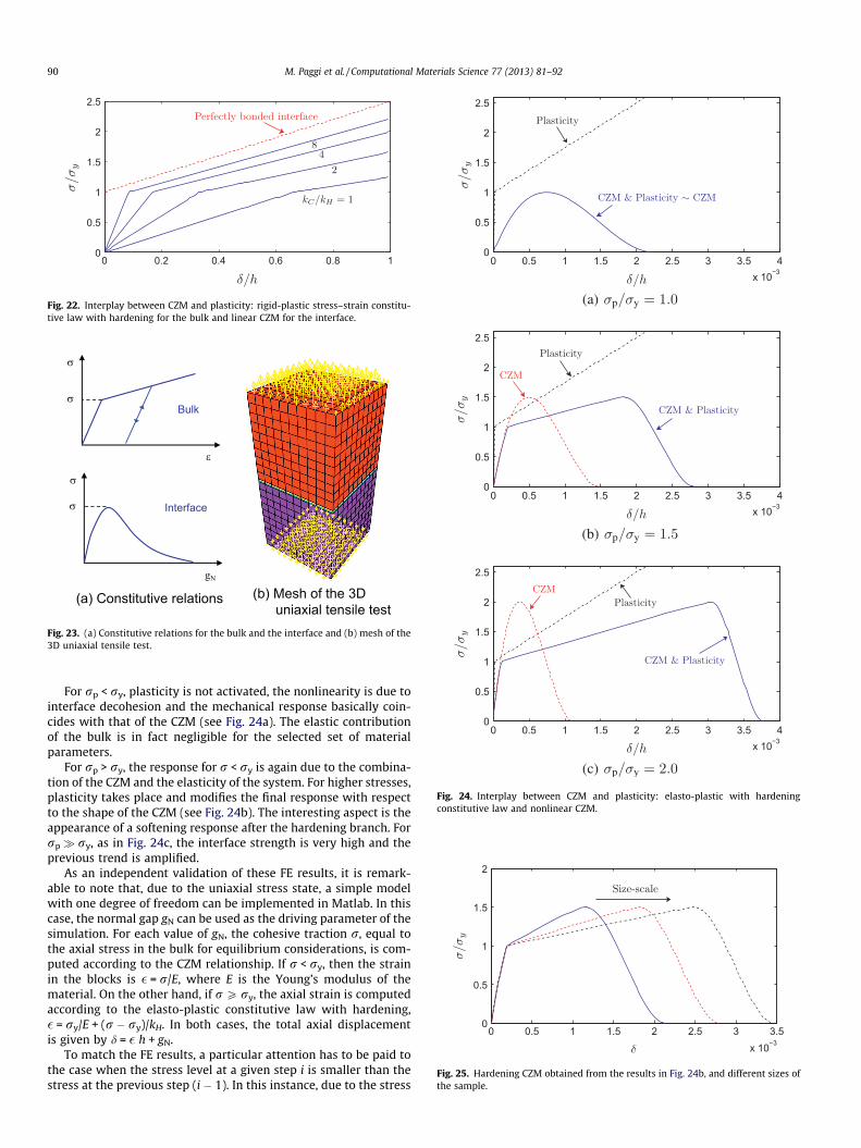
Regarding the constitutive models, we preliminary consider theblocks as rigid-plastic with hardening, defined by the strain hard-ening modulus kH, see Fig. 21a. Again for the sake of simplicity, thecohesive zone model (CZM) of the interface is linear with a tensioncut-off in correspondence of r = rp. As for linear springs, the CZM isdefined by the slope kC in the cohesive traction vs. separation dia-gram of Fig. 21b. These assumptions will permit to derive a closed-form solution to the problem that clarifies the mechanisms of theinterplay between the two nonlinearities.

During the tensile test, the stress field inside the bulk must be inequilibrium with the cohesive tractions along the interface, asshown in Fig. 20. For each value of the imposed displacement d,the strain is � = d/h, where h is the undeformed vertical size ofthe sample. Since the bulk material is perfectly rigid, the displace-ment d is totally absorbed by the interface. Hence, the relativeopening displacement is gN = d. For this separation level, the cohe-sive traction is equal to r = kCgN. If r < ry, then the representativepoint P � (d,r) of the mechanical response is determined. If, on theother hand, ry < r < rp, the plastic deformation of the bulk mate-rial has to be considered. In this instance, the total specimen defor-mation is given by:

d ¼ �hþ gN; ð32Þ

where gN = r/kC and � is related to the stress level by the isotropichardening equation:

r ¼ ry þ kH�: ð33Þ

Obtaining � from Eq. (33) and substituting it in (32), we obtain:

d ¼ r� ry

kHhþ r

kC; ð34Þ

which gives the unknown stress level for a given axial displacementd:

r ¼ dþ ryh=kC

h=kC þ 1=kH: ð35Þ

Finally, for r > rp, the interface cannot sustain tractions any longerand the specimen breaks in two parts.

Although Eq. (35) has been derived under various simplifiedhypotheses, the following general results can be deduced:

(1) The stress–displacement response depends only on the CZMin the range r < ry.

(2) A strong interplay between CZM and plasticity takes placefor r > ry.

(3) The stress at failure and the corresponding axial deformationis governed by the CZM which imposes a cut-off to thecurves in Fig. 22 for r = rp.

(4) The mechanical response depends on the size h of the sam-ple. For very small specimens ðh! 0Þ;r ¼ kHd and the

δ

Fig. 15. Deformation of the 2D model of the polycrystal, by increasing the imposed boundary displacement d until failure. Displacements range from blue (zero displacement)to red (maximum displacement). (For interpretation of the references to color in this figure legend, the reader is referred to the web version of this article.)

Fig. 16. Deformation at failure of the 3D model of the polycrystal. Displacementsrange from blue (zero displacement) to red (maximum displacement). (Forinterpretation of the references to color in this figure legend, the reader is referredto the web version of this article.)

Table 112 fcc slip systems according to [26].

�ma �sa �ma �sa �ma �sa �ma �sa

(111) ½01 �1� ð1 �1 �1Þ ½0 �11� ð�1 1 �1Þ [011] ð�1 �11Þ ½0 �1 �1�(111) ½�101� ð1 �1 �1Þ ½�10 �1� ð�1 1 �1Þ ½10 �1� ð�1 �11Þ [101](111) ½1 �10� ð1 �1 �1Þ [110] ð�1 1 �1Þ ½�1 �10� ð�1 �11Þ ½�110�

0.0

0.5

1.0

1.5

2.0

0 5 10 15 20δ/δy

F/F y

2D3D

Fig. 17. 3D vs. 2D simulation of plastic flow: dimensionless force vs. displacementcurves.

88 M. Paggi et al. / Computational Materials Science 77 (2013) 81–92

response is governed by plasticity only. For very largesamples, ðh!1Þ;r ¼ rykC=kH . Since kC� kH in practicalcases, it is easy to have kC/kH > rp/ry and therefore r > rp.Hence, for very large specimens, brittle cohesive failure isexpected to dominate over plasticity.

(5) In case of perfectly plastic materials (kH ? 0), no equilibriumsolutions can be found for r > ry.

(6) By increasing the ratio kC/kH, the mechanical response tendsto the rigid-plastic one, see the various curves in Fig. 22. Thelimit situation kC/kH ?1 corresponds to perfectly bondedinterfaces.

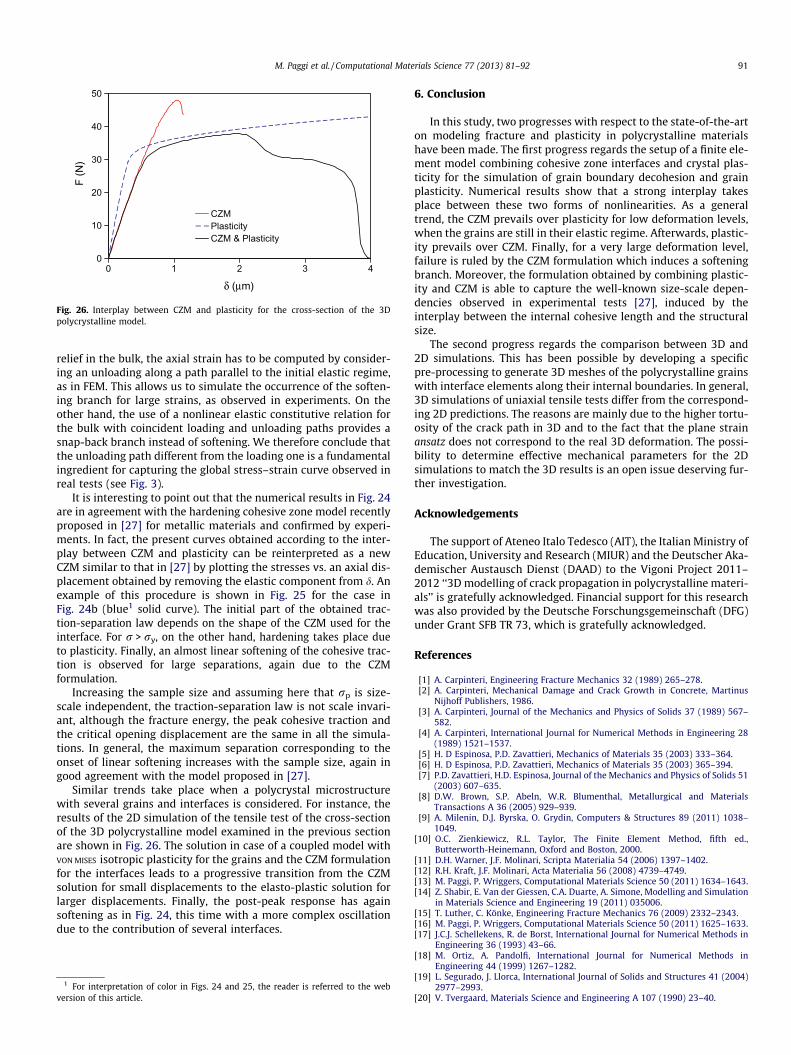
A more realistic scenario involving an elasto-plastic constitutivemodel for the bulk and a nonlinear softening CZM for the interface(see Fig. 23a) leads to a set of equations that cannot be solved inclosed form. However, it is possible to proceed numerically withFEM. The two blocks are discretized with quadratic brick elementsand compatible interface elements, see Fig. 23b. The axial test iscarried out under displacement control. An elasto-plastic constitu-tive model with hardening (E = 152000 MPa, ry = 80 MPa,kH = 120 MPa) is considered for the bulk material. Regarding thenonlinear CZM at the interface, the formulation in [20] is used witha fracture energy GF ¼ 0:1 N/mm and different values of rp.

δ/δy=0.1 δ/δy=1.0 δ/δy=20.0

Fig. 18. Cotour plot of the vertical component of the displacement field in the 3D polycrystal and deformed meshes. For each image, the scale ranges from blue (nodisplacement) to red (maximum displacement). (For interpretation of the references to color in this figure legend, the reader is referred to the web version of this article.)

δ/δy=0.1 δ/δy=1.0 δ/δy=20.0

Fig. 19. Contour plot of the vertical component of the displacement field in the 2D polycrystal. For each image, the scale ranges from blue (no displacement) to red (maximumdisplacement). (For interpretation of the references to color in this figure legend, the reader is referred to the web version of this article.)

Fig. 20. Sketch of the uniaxial tensile test.

(a) (b)Fig. 21. Constitutive laws: (a) rigid-plastic stress–strain curve for the bulk materialand (b) linear CZM with tension cut-off for the interface.

M. Paggi et al. / Computational Materials Science 77 (2013) 81–92 89

For rp < ry, plasticity is not activated, the nonlinearity is due tointerface decohesion and the mechanical response basically coin-cides with that of the CZM (see Fig. 24a). The elastic contributionof the bulk is in fact negligible for the selected set of materialparameters.

For rp > ry, the response for r < ry is again due to the combina-tion of the CZM and the elasticity of the system. For higher stresses,plasticity takes place and modifies the final response with respectto the shape of the CZM (see Fig. 24b). The interesting aspect is theappearance of a softening response after the hardening branch. Forrp� ry, as in Fig. 24c, the interface strength is very high and theprevious trend is amplified.

As an independent validation of these FE results, it is remark-able to note that, due to the uniaxial stress state, a simple modelwith one degree of freedom can be implemented in Matlab. In thiscase, the normal gap gN can be used as the driving parameter of thesimulation. For each value of gN, the cohesive traction r, equal tothe axial stress in the bulk for equilibrium considerations, is com-puted according to the CZM relationship. If r < ry, then the strainin the blocks is � = r/E, where E is the Young’s modulus of thematerial. On the other hand, if r P ry, the axial strain is computedaccording to the elasto-plastic constitutive law with hardening,� = ry/E + (r � ry)/kH. In both cases, the total axial displacementis given by d = � h + gN.

To match the FE results, a particular attention has to be paid tothe case when the stress level at a given step i is smaller than thestress at the previous step (i � 1). In this instance, due to the stress

0 0.2 0.4 0.6 0.8 10

0.5

1

1.5

2

2.5

Fig. 22. Interplay between CZM and plasticity: rigid-plastic stress–strain constitu-tive law with hardening for the bulk and linear CZM for the interface.

Fig. 23. (a) Constitutive relations for the bulk and the interface and (b) mesh of the3D uniaxial tensile test.

0 0.5 1 1.5 2 2.5 3 3.5 4x 10−3

0

0.5

1

1.5

2

2.5

0 0.5 1 1.5 2 2.5 3 3.5 4x 10−3

0

0.5

1

1.5

2

2.5

0 0.5 1 1.5 2 2.5 3 3.5 4x 10−3

0

0.5

1

1.5

2

2.5

Fig. 24. Interplay between CZM and plasticity: elasto-plastic with hardeningconstitutive law and nonlinear CZM.

0 0.5 1 1.5 2 2.5 3 3.5x 10−3

0

0.5

1

1.5

2

Fig. 25. Hardening CZM obtained from the results in Fig. 24b, and different sizes ofthe sample.

90 M. Paggi et al. / Computational Materials Science 77 (2013) 81–92

relief in the bulk, the axial strain has to be computed by consider-ing an unloading along a path parallel to the initial elastic regime,as in FEM. This allows us to simulate the occurrence of the soften-ing branch for large strains, as observed in experiments. On theother hand, the use of a nonlinear elastic constitutive relation forthe bulk with coincident loading and unloading paths provides asnap-back branch instead of softening. We therefore conclude thatthe unloading path different from the loading one is a fundamentalingredient for capturing the global stress–strain curve observed inreal tests (see Fig. 3).

It is interesting to point out that the numerical results in Fig. 24are in agreement with the hardening cohesive zone model recentlyproposed in [27] for metallic materials and confirmed by experi-ments. In fact, the present curves obtained according to the inter-play between CZM and plasticity can be reinterpreted as a newCZM similar to that in [27] by plotting the stresses vs. an axial dis-placement obtained by removing the elastic component from d. Anexample of this procedure is shown in Fig. 25 for the case inFig. 24b (blue1 solid curve). The initial part of the obtained trac-tion-separation law depends on the shape of the CZM used for theinterface. For r > ry, on the other hand, hardening takes place dueto plasticity. Finally, an almost linear softening of the cohesive trac-tion is observed for large separations, again due to the CZMformulation.

Increasing the sample size and assuming here that rp is size-scale independent, the traction-separation law is not scale invari-ant, although the fracture energy, the peak cohesive traction andthe critical opening displacement are the same in all the simula-tions. In general, the maximum separation corresponding to theonset of linear softening increases with the sample size, again ingood agreement with the model proposed in [27].

Similar trends take place when a polycrystal microstructurewith several grains and interfaces is considered. For instance, theresults of the 2D simulation of the tensile test of the cross-sectionof the 3D polycrystalline model examined in the previous sectionare shown in Fig. 26. The solution in case of a coupled model withVON MISES isotropic plasticity for the grains and the CZM formulationfor the interfaces leads to a progressive transition from the CZMsolution for small displacements to the elasto-plastic solution forlarger displacements. Finally, the post-peak response has againsoftening as in Fig. 24, this time with a more complex oscillationdue to the contribution of several interfaces.

6. Conclusion

In this study, two progresses with respect to the state-of-the-arton modeling fracture and plasticity in polycrystalline materialshave been made. The first progress regards the setup of a finite ele-ment model combining cohesive zone interfaces and crystal plas-ticity for the simulation of grain boundary decohesion and grainplasticity. Numerical results show that a strong interplay takesplace between these two forms of nonlinearities. As a generaltrend, the CZM prevails over plasticity for low deformation levels,when the grains are still in their elastic regime. Afterwards, plastic-ity prevails over CZM. Finally, for a very large deformation level,failure is ruled by the CZM formulation which induces a softeningbranch. Moreover, the formulation obtained by combining plastic-ity and CZM is able to capture the well-known size-scale depen-dencies observed in experimental tests [27], induced by theinterplay between the internal cohesive length and the structuralsize.

The second progress regards the comparison between 3D and2D simulations. This has been possible by developing a specificpre-processing to generate 3D meshes of the polycrystalline grainswith interface elements along their internal boundaries. In general,3D simulations of uniaxial tensile tests differ from the correspond-ing 2D predictions. The reasons are mainly due to the higher tortu-osity of the crack path in 3D and to the fact that the plane strainansatz does not correspond to the real 3D deformation. The possi-bility to determine effective mechanical parameters for the 2Dsimulations to match the 3D results is an open issue deserving fur-ther investigation.

Acknowledgements

The support of Ateneo Italo Tedesco (AIT), the Italian Ministry ofEducation, University and Research (MIUR) and the Deutscher Aka-demischer Austausch Dienst (DAAD) to the Vigoni Project 2011–2012 ‘‘3D modelling of crack propagation in polycrystalline materi-als’’ is gratefully acknowledged. Financial support for this researchwas also provided by the Deutsche Forschungsgemeinschaft (DFG)under Grant SFB TR 73, which is gratefully acknowledged.

References

[1] A. Carpinteri, Engineering Fracture Mechanics 32 (1989) 265–278.[2] A. Carpinteri, Mechanical Damage and Crack Growth in Concrete, Martinus

Nijhoff Publishers, 1986.[3] A. Carpinteri, Journal of the Mechanics and Physics of Solids 37 (1989) 567–

582.[4] A. Carpinteri, International Journal for Numerical Methods in Engineering 28

(1989) 1521–1537.[5] H. D Espinosa, P.D. Zavattieri, Mechanics of Materials 35 (2003) 333–364.[6] H. D Espinosa, P.D. Zavattieri, Mechanics of Materials 35 (2003) 365–394.[7] P.D. Zavattieri, H.D. Espinosa, Journal of the Mechanics and Physics of Solids 51

(2003) 607–635.[8] D.W. Brown, S.P. Abeln, W.R. Blumenthal, Metallurgical and Materials

Transactions A 36 (2005) 929–939.[9] A. Milenin, D.J. Byrska, O. Grydin, Computers & Structures 89 (2011) 1038–

1049.[10] O.C. Zienkiewicz, R.L. Taylor, The Finite Element Method, fifth ed.,

Butterworth-Heinemann, Oxford and Boston, 2000.[11] D.H. Warner, J.F. Molinari, Scripta Materialia 54 (2006) 1397–1402.[12] R.H. Kraft, J.F. Molinari, Acta Materialia 56 (2008) 4739–4749.[13] M. Paggi, P. Wriggers, Computational Materials Science 50 (2011) 1634–1643.[14] Z. Shabir, E. Van der Giessen, C.A. Duarte, A. Simone, Modelling and Simulation

in Materials Science and Engineering 19 (2011) 035006.[15] T. Luther, C. Könke, Engineering Fracture Mechanics 76 (2009) 2332–2343.[16] M. Paggi, P. Wriggers, Computational Materials Science 50 (2011) 1625–1633.[17] J.C.J. Schellekens, R. de Borst, International Journal for Numerical Methods in

Engineering 36 (1993) 43–66.[18] M. Ortiz, A. Pandolfi, International Journal for Numerical Methods in

Engineering 44 (1999) 1267–1282.[19] L. Segurado, J. Llorca, International Journal of Solids and Structures 41 (2004)

2977–2993.[20] V. Tvergaard, Materials Science and Engineering A 107 (1990) 23–40.

0

10

20

30

40

50

0 1 2 3 4

δ (μm)

F (N

)

CZMPlasticityCZM & Plasticity

Fig. 26. Interplay between CZM and plasticity for the cross-section of the 3Dpolycrystalline model.

1 For interpretation of color in Figs. 24 and 25, the reader is referred to the webversion of this article.

M. Paggi et al. / Computational Materials Science 77 (2013) 81–92 91

[21] D. Peirce, R.J. Asaro, A. Needleman, Acta Metallurgica 30 (1982) 1087–1119.[22] R.J. Asaro, A. Needleman, Acta Metallurgica 33 (1985) 923–953.[23] C. Miehe, International Journal for Numerical Methods in Engineering 39

(1996) 3367–3390.[24] J. Ruppert, Journal of Algorithms 18 (1995) 548–585.[25] J. Shewchuk, Tetrahedral mesh generation by Delaunay refinement, in: Proc. of

the 16th Annu. Sympos. Comput. Geom., 1998.

[26] J.L. Bassani, Plastic flow of crystals, in: J.W. Hutchinson, T.Y. Wu (Eds.),Advances in Applied Mechanics, vol. 30, Elsevier, 1994, pp. 191–258.

[27] A. Carpinteri, B. Gong, M. Corrado, Hardening cohesive/overlapping zonemodel for metallic materials: the size-scale independent constitutive law,Engineering Fracture Mechanics 82 (2011) 29–45.

92 M. Paggi et al. / Computational Materials Science 77 (2013) 81–92