applied sciences

Article

A Novel Way to Automatically Plan CellularNetworks Supported by Linear Programming andCloud Computing

André Godinho 1,2,* , Daniel Fernandes 1,2 , Gabriela Soares 3, Paulo Pina 1,2 ,Pedro Sebastião 1,2, Américo Correia 1,2 and Lucio S. Ferreira 3,4

1 ISCTE-IUL—Instituto Universitário de Lisboa, Av. das Forças Armadas 376, 1600-077 Lisbon, Portugal;dfsfs@iscte.pt (D.F.); paulo_pina@iscte-iul.pt (P.P.); pedro.sebastiao@iscte-iul.pt (P.S.);americo.correia@iscte-iul.pt (A.C.)

2 Instituto de Telecomunicações, Av. das Forças Armadas 376, 1600-077 Lisbon, Portugal3 Multivision—Consultoria, Rua Soeiro Pereira Gomes, Lote Nº1, 3ºC, 1600-196 Lisbon, Portugal;

gabrielasoares@gmail.com (G.S.); lucio.ferreira@multivision.pt (L.S.F.)4 INESC-ID/COPELABS-Universidade Lusófona, Campo Grande 376, 1749-024 Lisbon, Portugal* Correspondence: afgos@iscte-iul.pt

Received: 18 March 2020; Accepted: 22 April 2020; Published: 28 April 2020�����������������

Abstract: With the increasing number of mobile subscribers worldwide, there is a need for fast andreliable algorithms for planning/optimization of mobile networks, especially because, in order tomaintain a network’s quality of service, an operator might need to deploy more equipment. This paperpresents a quick and reliable way to automatically plan a set of frequencies in a cellular network,using both cloud technologies and linear programming. We evaluate our pattern in a realistic scenarioof a Global System for Mobile communications protocol (GSM) network and compare the resultsto another already implemented commercial tool. Results show that even though network qualitywas similar, our algorithm was twelve times faster and used four times less memory. It was alsoable to frequency plan seventy cells simultaneously in less than three minutes. This mechanismwas successfully integrated in the professional tool Metric, and is currently being used for cellularplanning. Its extension for application to 3/4/5G networks is under study.

Keywords: cellular-planning; cloud-services; implementation; integer linear-programming;monitoring; optimization

1. Introduction

By September of 2019, the number of mobile subscribers worldwide was around 8 billion, and oneestimation puts that number at 8.9 billion by 2025 [1]. This means that in order to maintain thenetwork’s capacity and its quality of service (QoS), one might need to deploy more equipment,increasing the risk of a chaotic network, and consequently, the amount of interference.

Wireless cellular networks propagate electromagnetic waves to establish connectivity betweenbase station (BS) antennas and users’ mobile terminals. Multiple antennas must be deployed toprovide coverage of a given service area. To operate, mobile operators have access to a set of radiochannels, frequencies with specific bandwidths allowing them to establish communication with mobileterminals. The distribution of frequencies among BSs, so-called frequency planning, is a challenge,as the re-use of the same frequency by a neighboring cell may result in interference that makes itimpossible to communicate.

Usually, frequency planning and allocation is a manual, time consuming, but important task toa quality network. The reason for the complexity of this task is because of aspects such as terrain

Appl. Sci. 2020, 10, 3072; doi:10.3390/app10093072 www.mdpi.com/journal/applsci

Appl. Sci. 2020, 10, 3072 2 of 20

topography and urban density, where non-uniform coverage exists. The overall objective is to allocatefrequencies while creating the least amount of interference—ideally, none.

There are protocols that can be applied to help with solving this problem. Self-organizingnetworks (SON) are an example of that. They collect data from the network and automatically makechanges to it based on that data, by analyzing a set of key performance indicators (KPIs). In our case,we would need a KPI representing interference. Interference is possible to estimate, using estimatedcell powers from propagation models such as Okumura-hata and Walfish Ikegami [2].

This idea is applied and tested for the Global System for Mobile communications protocol(GSM), a cellular system that, compared to UMTS and LTE, presents higher challenges in terms ofcellular planning [3]. GSM specifies that a cell has to have both control channels (CCH) and trafficchannels (TCH), responsible for transmitting network information and user traffic respectively.

This new planning pattern was implemented and applied in a commercial tool called Metric [4].Metric is a planning, monitoring, and optimizing tool for mobile networks, currently used bymultiple operators.

The novelty of this paper is the use of cloud services and linear programming to quickly andautomatically plan or heal a network. Following the SON concept, we were able to create andimplement a work pattern which estimates power, calculates possible interference, and finds a solution,outputting the best set of frequencies to allocate to each cell.

This paper considered the possibility of mass planing new cells from different sites. New methodsand materials were used, new optimization rules and evaluation tests were obtained, and the newfunctionalities were introduced in the Metric tool. This work was started by the work presentationin [5] considering new gaps and opportunities to plan mobile cellular networks in an efficient wayassuring the accuracy and precision of results.

The paper is organized as follows: Section 2 presents the state-of-the-art and related work, includingthe methods and materials used. We also mathematically explain our definition of interference, as wellas other rules used in integer linear programming. In the same section we also detail all modulespecifications and implementations present in the working pattern. The evaluation scenario and testsresults are described in Section 3. Finally, main conclusions and future work are described in Section 4.

2. Materials and Methods

In the next sections, we will briefly talk about the concepts related to and used in our work.In Section 2.1 we explain cell coverage, interference, and types of planning. Next, we explain theconcept of SON in Section 2.2. We then talk about cloud services and the types of serverless computingin Section 2.3. In Section 2.4 there is a small explanation of Metric software as a service (SaaS).The Z-order curve and the Geohash algorithm are explained in Section 2.5. Finally, we talk about linearprogramming in Section 2.6.

2.1. Cellular Planning

Cellular planning is important in order to increase network capacity and avoid interferencebetween the increasing number of active devices in an area. A good plan not only reduces networkcosts, but also increases the quality of service. Ideally, the coverage area should be uniform, withoutoverlaps or empty spaces. One can theoretically solve this problem using regular polygons (triangles,squares, and hexagons). The hexagon is most-often used because it is the polygon closer to the realcoverage of an omnidirectional antenna. Problems begin to appear when one understands that thereal coverage might not be close to a hexagon at all, as illustrated in Figure 1. Aspects like terraintopography and urban density change the way power decays over time. Another problem is thattraffic distribution is not uniform. Different cell sizes must be used—smaller ones for areas with moretraffic and vice-versa. In consequence, the network becomes less and less uniform.

Appl. Sci. 2020, 10, 3072 3 of 20

Figure 1. In the left, theoretical coverage; on the right, a real coverage example.

Knowing this, there are three types of interference [6] which we need to account for:

• Co-channel interference: The interference created from other cells with the same frequency. This issolved by spacing cells with the same frequency and splitting the cell in sectors (sectorization).

• Adjacent Interference: The interference coming from adjacent channels in adjacent cells. This iseasily solved with quality filters and making sure there are sufficient differences between thefrequencies used in those cells.

• Self interference: A consequence from a cell’s signal reflecting from obstacles (buildings, mountains,etc.). Solved by correctly splitting downlink and uplink frequencies.

There are multiple ways to allocate frequencies. The most used are either fixed frequencyallocation, where frequency allocation respects a set of constraints as well as possible, and minimumspan allocation, where allocation is done using the minimum amount of frequencies still respectingthose constraints. But there are other “out of the box” solutions. In 2010, Chao et al. [7] proposeda new method of frequency planning using a cell’s latitude, longitude, and azimuth, and comparingthem with that cell’s neighbors, thereby predicting which cells will interfere with each other. However,this process is still manual and requires human intervention.

2.2. Self-Organizing Networks

Usually, mobile network design requires three phases. First is network planning, taking in accountcertain aspects such as coverage, interference, quality of service, and frequency reusing. Second comesmonitoring: using KPIs to evaluate the current state of the network. Those KPIs are analyzed in thefinal phase, optimization, changing parameters such as cell direction and intensity, antenna height,and radio parameters. This process its manual, expensive, and time consuming. In order to solvethese problems, an automated technology named SON was designed in order to automatically plan,configure, manage, optimize, and heal mobile networks. This technology is characterized by a lifecycle (Figure 2) composed of three phases:

• Self-configuration: Following the idea of “plug and play,” this section is responsible forconfiguring a new node in a network, not only in connectivity but also for transferring thenetwork parameters to that node.

• Self-optimization: Responsible for important factors in the network, such as topology,propagation, and interference (the one which is covered in this paper).

• Self-healing: In case some nodes fail. This section is responsible for warning the other nodes ofthat failure in order to reduce the impacts on the network’s services.

Appl. Sci. 2020, 10, 3072 4 of 20

Figure 2. A self organizing network’s life cycle.

2.3. Cloud Services

Cloud services make it so that someone can connect and use applications based in the cloud. Thereare multiple advantages. Both users and companies can have access to complex applications withoutthe need for specialized hardware/software. Not only that though, as users can usually access thoseapplications on any device with internet access, which also means that all data are the same, regardlessof that device. Finally, those applications are usually pay-per-use, avoiding expenses on unusedservices. Usually, the amount paid for these services is lower than the amount paid for management ofdedicated hardware [8]. The clear definition and application of the service level agreement (SLA) areof paramount importance. Cloud-based solutions are only viable for a client if aspects such as qualityand availability are defined between him and the service provider [9]. One example is Amazon WebServices (AWS), which contains services and applications in areas including databases, virtual servers,computation, machine learning, artificial intelligence, gaming, internet of things, and many others [10].

As illustrated in Figure 3, there are three standard types of service modules, each one defined bythe National Institute of Standards and Technology (NIST) [11]:

• Infrastructure as a service (IaaS): Where the consumer is able to deploy and run arbitrary software,which can include operating systems and applications. The consumer does not manage or controlthe underlying cloud infrastructure but has control over operating systems, storage, and deployedapplications; and possibly limited control of select networking components (e.g., host firewalls).

• Platform as a service (PaaS): The capability provided to the consumer is to deploy onto the cloudinfrastructure consumer-created or acquired applications created using programming languages,libraries, services, and tools supported by the provider. The consumer does not manage orcontrol the underlying cloud infrastructure including network, servers, operating systems,or storage, but has control over the deployed applications and possibly configuration settings forthe application-hosting environment.

• Software as a service (SaaS): The capability provided to the consumer is to use the provider’sapplications running on a cloud infrastructure. The applications are accessible from variousclient devices through either a thin client interface, such as a web browser (e.g., web-basedemail), or a program interface. The consumer does not manage or control the underlying cloudinfrastructure including network, servers, operating systems, storage, or even individual applicationcapabilities, with the possible exception of limited user-specific application configuration settings.

Appl. Sci. 2020, 10, 3072 5 of 20

Figure 3. Cloud computing business model [12].

Another service model is function as a service (FaaS), also associated with serverlesscomputing [13]. Instead of using a continuously working virtual machine, FaaS enables the deploymentof single functions which are only executed after a trigger or an event. This might be a better alternativefor running code which does not have to execute multiple times or/and for a long time. One exampleof FaaS is AWS Lambda. [14].

2.4. Metric SaaS and Other Commercial Tools

Metric SaaS is software as a service for commercial use, created and maintained by Multivision Lda.This service allows easy access of network data, reports, and issues, to everyone in a team. Networkdata, such as “RxLevel,” “Interference,” cell frequency, and many others, can not only be visualized ona map (Figure 4), but also imported to any system.

Figure 4. Metric SaaS map interface, highlighting the available 2G cells geolocated in the terrain.

Metric already has integration for SON in both monitoring and maintenance. Our objectiveis to add the integration in optimization by automatically calculating interference and the bestfrequency allocation.

There are different commercial tools used in mobile network design. For example, WinProp isable to accurately simulate propagation data of cells in multiple environments, such as rural, urban,indoor, and underground [15]. However, it lacks other planning tools like neighbors lists.

Atoll is one of the most used by operators [16]. It runs as a local application with some installationsopting for connectivity to external databases that are outside of the application scope license. The user

Appl. Sci. 2020, 10, 3072 6 of 20

needs, at least, an up-to-date machine with the minimum capacity to plan a set of cells in a reasonableamount of time. Although we do not have access to the application internals, its modus operandisuggests that it follows some type of simulated annealing implementation where time invested incomputation translates into an improved frequency planning. This approach looks like a planninggamble and it would be interesting to see whether the product produces different results with differentparameterization seeds running in multiple machines in parallel, but we pushed this type of analysisaway for future benchmark work. Nevertheless, we acknowledge the strategic option, since withsuch limited resources and without the possibility of scaling the computation horizontally, it isa reasonable compromise.

Mentum Planet nowadays is part of the InfoVista tool panoply [17]. It does not suffer from thelocal limitations of a single machine, but it is still bound to an on-premises infrastructure that theuser needs to setup up-front. It is possible to integrate multiple data sources, but Planet is basicallya bunch of build-stitching tools and services that InfoVista acquired along its path to conqueringa larger market share. The stitching of different technologies created a tool hard to use, one plaguedwith a licensing plan very hard to grasp even for the most basic usage. A user that only wants toevaluate the suite for frequency planning should accept a slow learning curve.

2.5. Z-Order Curve and Geohash

At a certain point in our implementation, we had to uniformly identify geographic areas aroundthe world. Z-order curve is an algorithm which converts multidimensional data in unidimensionalwithout losing original information. It was created and first used by Guy Macdonald Morton for filesequencing in 1966 [18]. Basically, the transformation is done by interleaving the binary representationsof each coordinate, as illustrated in Figure 5. There are multiple applications of the Z-order curve,including linear algebra [19,20], texture mapping, image/video encoding, and quadtree generation [21].

Figure 5. Using Z-order curve to interleave binary representations of integers between 0 and 7, inclusive.

Appl. Sci. 2020, 10, 3072 7 of 20

Gustavo Niemeyer used this function on the invention of Geohash [22], a geographic encoderthat transforms geographic coordinates in a unique hash representing them. Although, soon it wasnoticed that there were other applications for its use, as it began being used for unique identifiers andpoint data representations in databases, for example, in MongoDB [23]. The size of this hash definesits precision; the larger its size the better its precision (Table 1).

Table 1. Geohash length and its precision with geographic coordinates.

Geohash Length Cell Width [km] Cell Height [km]

1 5000 50002 1250 6253 156 1564 39.1 19.55 4.89 4.896 1.22 0.617 0.153 0.1538 0.0382 0.01919 0.00477 0.00477

10 0.00119 0.000595

There are some problems in the Geohash algorithm. Usually, one can use Geohash prefixes to findpoints in proximity with each other. The first problem is that, in edge case locations, those prefixesare not similar at all. For example, “s0000” and “kpbpb” are adjacent geohashes, but since they are indifferent halves of the world (north of the equator and south of the equator respectively), their prefixesare not similar. The second problem is the lack of linearity in the Geohash distance representation ofour planet, since single degrees in latitude and longitude represent different distances. At the equatorthere is an error of 0.67%, at 30 degrees latitude there is an error of 14.89%, and at 60 degrees there isan error of 99.67%, tending to infinity the closer one goes to the poles. The source of this problem isnot Geohash itself but the difficulty of converting coordinates on a sphere to a unidimensional value.

2.6. Linear Programming

Linear programming, or linear optimization, is a method whose objective is to find the bestoutcome of a mathematical model using linear constraints. Linear programming was already usedin the past for channel allocation in large and cellular and radio networks [24]. Even though thisis a powerful tool, learning linear programming is time consuming, especially for people with noprogramming/mathematical background.

There are multiple linear programming solvers available, although most of them are either paidor have proprietary licenses. We analyzed some Copyleft licensed software, including Coin-or linearprogramming (CLP), GNU Linear Programming Kit (GLPK), Cassowary constraint solver, Lp_Solve,and Qoca. Even though GLPK appeared to be one of the least efficient (especially when compared tocommercial solvers) [25,26], it had the advantage of an already available layer for AWS Lambda [27].

There are also multiple input formats. For GLPK in particular, there are four:

• CPLEX-LP: Used in IBM ILOG CPLEX Optimization Studio, a commercially available optimizationsoftware package. More user-friendly than the others.

• MPS: Mathematical Programming System is a file format used in both linear programmingand mixed integer programming problems. There are some limitations though; for example,numeric fields limited to 12 characters. Modern extensions of this format, without those limitations,are also accepted by GLPK.

• GLPK: A custom format, similar to DINAMICS format, a format created by the Center for DiscreteMathematics and Theoretical Computer Science;

Appl. Sci. 2020, 10, 3072 8 of 20

• MathProg—High level modelling language. GLPK MathProg translator is not appropriate forlarge models, due to its taking a considerable amount of time with big problems. This happensbecause the translator is not able to recognize shortcuts on the optimization.

We ended up using the MathProg format, since the models are not that big and it is possible tostructure it, cluing the solver in on optimization paths for faster optimization. In case someone findsa model to take a long optimization time, they can use GLPK to convert a MathProg format in any ofthe other formats. There are cases where converting first and optimizing later is more efficient.

2.7. Optimization Algorithm for Planning

Within frequency planning, the main goal is that the set of channels allocated to each cellminimizes interference. For a given geographic position, the carrier to interference ratio (C/I) measuresthe ratio between the cell’s signal power level and the sum of power levels of cells operating in the samefrequency. A system is only capable of operating above a minimum value, C/Imin. An interferenceregion, depicted in Figure 6, is characterized by C/I levels below C/Imin, an area where communicationis not possible in the evaluated frequency.

Figure 6. Illustration of the received signal level decay with distance for two neighboring cells:the corresponding interference region is identified.

The proposed algorithm evaluates, for each unplanned cell c, the interference experienced whenoperating on each of the available BCCHs, the best server cell, c f ,b, shall correspond to the cell withstrongest received signal level, Prx. Remaining cells operating in f with signal present in pixel ppp arethe set of non-best server cells, ±c f ,nb. Thus, a given covered pixel ppp of c is labeled as interfered if C/Iis below C/Imin:

Prx(ppp, c f ,b)

∑c f ,n∈ccc f ,nbPrx(ppp, c f ,nb)

< (C/I)min (1)

where Prx(ppp, c f ,b) (mW) is the received signal power level in pixel ppp of best server cell c f ,b;Prx(ppp, c f ,nb) (mW) is the received signal power level in pixel ppp of non-best server cell c f ,nb, belongingto ccc f ,nb set; and (C/I)min is the minimum C/I level that guarantees interference free communication.In GSM this value is typically taken as 9 dB.

For the unplanned cells set, ccc, and the set of sorted frequencies, fff , DDD matrix is built. It hasdimension dim(ccc)× dim( fff ), having for each cell and frequency the number of pixels with interference;i.e., where condition (1) is observed. The objective is to minimize interference, given mathematically by:

min ∑c∈ccc

∑f∈ fff

DDDc f ×XXXTc f (2)

where XXX is a Boolean matrix with similar dimensions as DDD.

Appl. Sci. 2020, 10, 3072 9 of 20

When various cells of different sites shall be planned, the amount of possible interferencecreated by unplanned cells that share the coverage area is also minimized, in case these cells getthe same BCCH:

min ∀ f ∈ fff and ∀c1, c2 ∈ ccc :(XXXc1 f +XXXc2 f

)×UUUc1c2 (3)

where UUUc1c2 is “1” if cells c1 and c2 interfere, and “0” otherwise. Two cells operating in the same BCCHinterfere with each other when there are pixels covered by c1 that are interfered by c2. Nevertheless, thisrestriction shall be relaxed. In fact, the solution to this optimization problem may not be the best oneor might even return a solution as impossible. Ideally, UUUc1c2 , would become an integer, representingthe number of pixels in c1 interfered by c2. This minimization was originally a condition, but aftersome research on integer programming heuristics, we concluded that this way the optimization wouldbe much faster (from hours to under a second, when optimizing 50 cells).

When planning frequencies, certain rules must be followed. These are expressed by a set ofrestrictions to the optimization problem. First, a single BCCH must be allocated to each unplanned cell:

∀c ∈ ccc : ∑f∈ fff

XXXc f = 1 (4)

Secondly, cells of the same site sss (which may contain both planned and unplanned cells), cannotreuse the same BCCHs:

given sss, ∀ f ∈ fff : ∑c∈sss

XXXc f ≤ 1 (5)

Thirdly, the cells of sss cannot have adjacent frequencies. The sorted set of frequencies fff is indexed,starting in index 0 and going until index dim( fff ). This restriction can be expressed mathematicallyas follows:

∀ fi, i ∈ [1, dim( fff )] : ∑c∈sss

(XXXc fi−1

−XXXc fi

)≤ 1 (6)

Regarding the planning of TCH, each cell has several TCH frequencies allocated. The same set ofrules is applied to the optimization of TCH frequencies, with the exception that there needs to be atleast a difference of two frequencies between TCHs of the cells of the same site:

∀ fi, i ∈ [1, dim( fff )] : ∑c∈sss

∑t∈tttc

(XXXt fi−2

−XXXt fi−1−XXXt fi

)≤ 1 (7)

where tttc identifies the set of available TCH channels of cell c.

2.8. Architecture

The architecture of our working pattern, as depicted in Figure 7 is basically a group of fourmodules linearly connected. The fact that it is cloud based not only allows us to communicate with thecellular network operation support system (OSS), but also, one can use each module individually foranother reasons besides frequency planning.

Each module represents a processing service, while between each module will be a storage service,to save any inputs/outputs. We implemented four different processes:

• Cell coverage estimation module: Responsible for estimating a cell power around its location.• Cell grid intersections module: Responsible for understanding which cell coverage intersects.• World map creation module: Responsible for creating a world map, which is a data structure

containing a set of pixels identified by their hashes—in this case, Geohashes. Each pixel will havean undefined number of pairs of cell/power.

• Planning module: Responsible for applying a linear optimization and its defined rules to thedata generated by the previous modules.

The four steps of the pattern are detailed in the next sections.

Appl. Sci. 2020, 10, 3072 10 of 20

Figure 7. RAN architecture, integrating the proposed cloud-based work pattern for network monitoringand planning.

2.9. Cell Coverage Estimation Module

An algorithm that was created by Fernandes et al. [28]. It uses drive tests (DT)—tests done,usually in a vehicle, to obtain coverage data in an area and evaluate its quality—to calibrate a standardpropagation model (SPM) [29]. This module, given information recovered from Metris SaaS, suchas an antenna diagram, cell information, DTs, and altimetry data extracted from OpenTopography,outputs a propagation grid with power estimation on areas covered by the cell, as depicted in Figure 8.

Figure 8. Representation of the antenna’s received signal level estimation, calibrated with drive tests.

2.10. Cell Grid Intersection Module

A simple module computes a list of cells whose coverage intersects with the one being computed,as depicted in Figure 9. It takes on the pessimistic perspective, by drawing an imaginary rectanglewhere the coverage fits in and checks whether those rectangle borders intersect with any neighboringones. Depending on the lists’ sizes, it has two operational modes: computing the lists using a quadtree to make small lists and computing the potential intersection between all of them for larger lists,since the construction of a quad tree is computationally heavy.

Appl. Sci. 2020, 10, 3072 11 of 20

All data from this and the previous module were compiled and processed in the World mapcreation module (Figure 10).

Figure 9. Illustration of the cell intersection module, to identify neighboring cells of A, and the worldmap creation module, identifying for each pixel the received signal levels of neighboring cells.

Figure 10. Flowchart representing the algorithm workflow.

2.11. World Map Creation Module

It is common sense that a computer works better with discrete data, rather than continuous data.Knowing this, it is important to find a way to uniformly and coherently split the world into smallareas, in order for us to be able to compare cell powers in mutual areas and check for interference,as illustrated in Figure 9.

As explained in Section 2.5, Geohash covered our requirements; even though there is an increasingerror the closer we go to the poles, this is not significant, since we only care that the area betweendifferent cells that are both in the exact same space and have the exact same size.

This module generates a world map. A world map is a data structure containing pixelsrepresenting the area covered by our problem (area covered by all cells we are trying to plan).We compute each propagation grid mentioned in Section 2.9 of each cell participating in our problem,all of which were identified by the lists created in Section 2.10.

The module outputs a Tab-Separated Values (TSV) file representing a map, where each line isidentified by a Geohash, followed by pairs of cell/power. With this we can easily identify which cellsare in a certain area and their corresponding powers. We tried other file types and structures, but uponsome testing, we noticed that all the others would either take up more space and/or were too slow torealistically process.

2.12. Planning Module

Iterating trough the world map, pixel by pixel, we calculate whether the C/I is enough to maketelecommunication services unusable in that area. At the same time, a table with unplanned cells asrows and frequencies as columns is populated with the size of the area interfered with. Another table isalso populated to check interference between unplanned cells if they end up having the same frequency.

Appl. Sci. 2020, 10, 3072 12 of 20

These tables, in conjunction with the equations described in Section 2.7, are sent to the optimizer,which returns the best solution to the given problem.

2.13. Technology Used

This program is part of the automatic GSM frequency planning package Cloud-based PixelizedSite Planning (CPSP), within the Metric SaaS ecosystem [4]. It was written completely in Java 8 [30]and compiled by Maven [31], and each module is packaged into executable JARs which are hosted inAWS Lambdas, a serverless computing platform provided by Amazon Web Services (FaaS) [10].

We discussed the possibility of hosting the executables in another service call Elastic ComputerCloud (EC2), an infrastructure as a service, but we came to the conclusion that each of our moduleswas not supposed to run continuously; they were supposed to only run when needed, either becauseof a trigger or a call. If we used EC2 we would be paying continuously for the service, even if wewere not using it—the opposite to AWS Lambda. Using AWS cloud services also allowed to integrateour implementation, described in Section 2.8, in Metric SaaS. Currently, a user requests to plan GSMfrequencies in its interface.

All Lambda inputs/outputs are streamed/saved in S3 buckets, a storage service (PaaS).Finally, as explained in Section 2.6, we use GLPK solver (GLPSOL), to solve models in

MathProg format.

2.14. Implementation of the Work Pattern

In Figure 11 is detailed the pattern that implements the proposed framework using AWS Services.It receives information from the OSS and returns a set of frequency allocations to each cell we aretrying to plan. We can also see in the same figure that between each Lambda, all processed data aresaved in S3 buckets whose IDs depend on the client information. This data include but are not limitedto: propagation grids, intersection files, world maps, interference matrixes, cell configurations, andother client data.

Figure 11. AWS cloud services integration on work pattern.

Each lambda receives a JSON file as input. In this case, the file must have the names of thecells we want to plan, the frequency to which they must be planned as designed by the International

Appl. Sci. 2020, 10, 3072 13 of 20

Telecommunication Union (ITU) in GSM operations, and client information for file access, which isautomatically input based on the login session.

There are some restrictions about each individual lambda one needs to take into account:

• Maximum memory allocated is 3008 MB;• Timeout of 900 s (15 min);• Virtual storage is limited to 500 MB.

This is important because the world map can take a considerable amount of space; therefore,the implementation of streaming when reading a world map is a must. The same happens whenuploading a file to a bucket, since the file must first be created in Lambda’s temporary storage andonly then uploaded. Problems might appear when planning a large problem, where the optimizationcan take a long time.

Another possible problem was the fact that S3 buckets have a limit of 5 TB per object, but thatdoes not compare to the 500 MB of Lambda virtual storage, meaning that it can be ignored. There isalso a limit of 100 buckets (1000 with premium) per account, which again is not a problem, since wewould need five at max.

In Figure 11 we have the following AWS lambdas:

• Cell coverage estimation and grid generation AWS Lambda (L1): Using client informationimported from a S3 bucket (B0), this lambda creates a pixelized grid with coverage informationaround an antenna. This coverage is calculated using propagation modules, drive tests, andother cell parameters, such as elevation, azimuth, and tilt [32]. Those grids will be saved in an S3bucket (B1);

• Intersections AWS Lambda (L2): Using a metadata file imported from B1, L2 compiles that dataverifying which cells’ coverage intersects, by getting two opposite max distance corners. Finally,it outputs that data in a CSV file to B2.

• World Map AWS Lambda (L3): This lambda is responsible for creating a TSV file with Geohashkeys and pairs of cell/power, which we call a “World Map.” Both those grids and the map musthave the same Geohash precision (BitSet size) in order to avoid scale/localization incoherence.First, we use the intersection files from B2 to iterate trough the set of cells that we are trying toplan and find the corresponding intersection files. A new set of cells is created that includes allthe cells that intersect the ones we are trying to plan. We use the propagation grids of those cells(imported from B1) to compile and create a world map containing all those cells. At first, we triedto use a Json file, but its size ended up being too large to read in a reasonable amount of time.

• Planning AWS Lambda (L4): First, we count both the amount of interference in the world map,and the amount of possible interference in the case in which the unplanned cells end up withthe same frequency. Reminder that interference is defined by Equation (1). All data are writtenand sent to the GLPSOl module from GLPK library [33], a linear solver, in a “mathProg” file.In that file is also written the solver’s objective (Equation (2)) and all rules (Equations (3)–(7)).The outputted solution should have multiple x[c, f ] where x equals either 1 or 0. In case of theformer, it means that frequency f should be attributed to cell c. That data are exported usinga regex—“\[(\d+),(\w*)\]\s?\W*1”—computed, and sent back to the user.

All S3 file requests are made by reading the stream from the online connection to an S3 bucket,without the need to save the information in temporary files and avoiding the possible problem of usingmore than the available 500 MB of temporary storage.

2.15. Integration in Metric

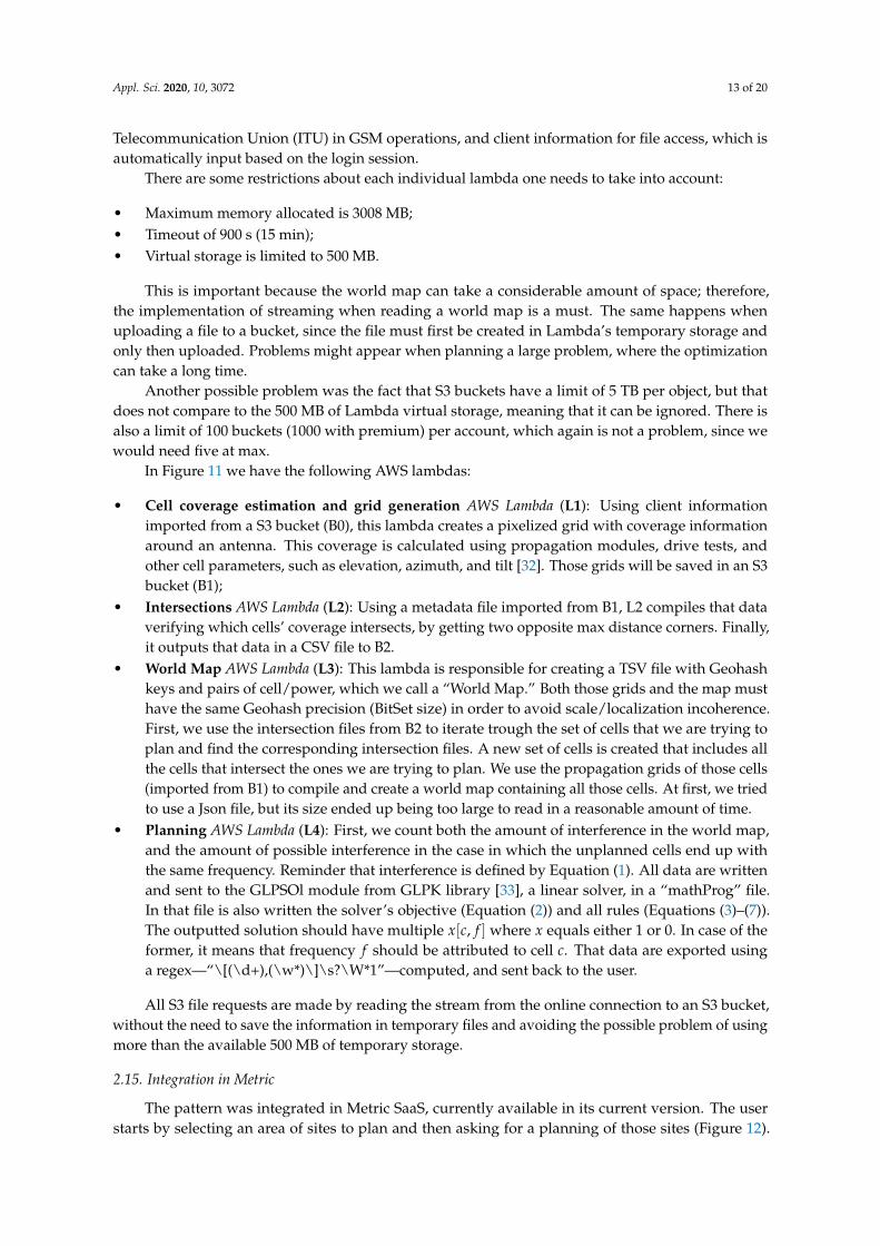
The pattern was integrated in Metric SaaS, currently available in its current version. The userstarts by selecting an area of sites to plan and then asking for a planning of those sites (Figure 12).

Appl. Sci. 2020, 10, 3072 14 of 20

The system then sends a request to AWS Web services, which after processing the data returns the bestplanning to that area.

Figure 12. Frequency allocation request in Metric SaaS.

3. Experiment, Results, and Discussion

In the next sections, we will set the evaluation scenario and discuss both the experiments doneand their results.

3.1. Evaluation Scenario

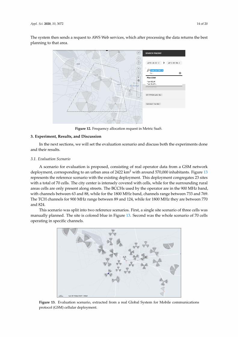
A scenario for evaluation is proposed, consisting of real operator data from a GSM networkdeployment, corresponding to an urban area of 2422 km2 with around 570,000 inhabitants. Figure 13represents the reference scenario with the existing deployment. This deployment congregates 23 siteswith a total of 70 cells. The city center is intensely covered with cells, while for the surrounding ruralareas cells are only present along streets. The BCCHs used by the operator are in the 900 MHz band,with channels between 63 and 88, while for the 1800 MHz band, channels range between 733 and 769.The TCH channels for 900 MHz range between 89 and 124, while for 1800 MHz they are between 770and 824.

This scenario was split into two reference scenarios. First, a single site scenario of three cells wasmanually planned. The site is colored blue in Figure 13. Second was the whole scenario of 70 cellsoperating in specific channels.

Figure 13. Evaluation scenario, extracted from a real Global System for Mobile communicationsprotocol (GSM) cellular deployment.

Appl. Sci. 2020, 10, 3072 15 of 20

3.2. Implementation Results and Discussion

After some initial simple assessment tests, the model was applied to our evaluation scenario.Initially, we tested the planning of the site with three cells. We generated with the C/I of eachpixel covered by that site: one with the original operator frequency planning, before optimization(Figure 14a) and after the CPSP planning (Figure 14b). The implementation in Metric was also used toassess the results of the proposed methodology. It runs in a physical machine while the proposed CPSPis cloud-based. Additionally, in terms of propagation, it uses the Okumura–Hata model to estimatereceive power levels, requiring larger computation resources, as will be shown. It splits the “world”using angles and distances, creating a non-uniform grid. A strong limitation of the Metric algorithm isthat its constraints only apply when planning cells from the same site. In this sense, planning a networkwith multiple sites can only be done sequentially, resulting in a non-optimal global solution.

(a) Before optimization. (b) After optimization.Figure 14. Carrier to interference ratio within the coverage area of the planned site.

An empirical cumulative distribution function is generated, as represented in Figure 15, in orderto compare network quality. Keep in mind that this distribution does not take in account pixels wherethe power of the most potent cell is not enough to enable connectivity, as the quality of the planning ofthe frequencies is not affected by it. Both CPSP and Metric plannings, even though they had differentfrequencies allocated, achieved similar network quality, as can be verified in Figure 15, and in anidentical heatmap, Figure 14b. Before optimization, the manual planning depicted in Figure 14aachieved 83.7% of the coverage area and below (C/I)min (9 dB). The bad quality of the area is visibleby the average C/I of 7 dB. After planning, we can observe in Figure 15 that 99.9% of the coveragearea is above 15 dB (6 dB higher than (C/I)min), enabling communication with excellent quality.

Figure 15. Cumulative distribution function of the C/I within the coverage area of the planned site.

Appl. Sci. 2020, 10, 3072 16 of 20

For the scenario in under analysis, the proposed CPSP planning algorithm is compared to theone of the Metric tool. Even though both achieve similar results, as is visible in Figure 15, theirperformances are different, in terms of execution time and memory usage efficiency, as depicted inFigure 16. For planning three cells, the proposed algorithm used up 985 MB of memory, taking 27.7 sto execute, an improvement compared to the 4096 MBs used and 329.2 s from the already implementedone. The proposed algorithm is almost 12 times faster and four times less memory consuming. Theseresults exclude the time and memory used to calculate the pre-processed propagation grids, which arepre-processed and available by Metric SaaS. Both the memory and time reduction can be explained bythe more uniform world division and by the fact that the world map is generated once instead of inmultiple individual generations for each cell.

Figure 16. Performance comparison between the proposed CPSP planning algorithm and the one ofMetric tool, in terms of execution time and memory usage.

We then applied the algorithm to the whole scenario of 70 cells, in order to check how the patternwould behave when planning multiple sites, taking 161.6 s and using 1439 MB of memory (Figure 17.We cannot compare it to metric since it can only plan a site at the time, but it could plan each siteindividually, one by one, taking 70 times 329 s (23,044 s). This approach has another major problem.The obtained solution might not be the best one because of the planning order.

Figure 17. Carrier to interference ratio in the city after optimization.

The proposed procedure is composed of searches in the world map, a hashtable and linearoptimization. For the next results, “World map” covers everything from reading the required files for

Appl. Sci. 2020, 10, 3072 17 of 20

generating the world map, to the process of sending the problem to optimization. The complexityof search on a hashtable is O(n), and the LP used has a time complexity of poly(n) [34]. Therefore,the proposed procedure is also poly(n). To illustrate and confirm that, we show in Figure 18 that,even though it looks linear, the best approximation for the time complexity is polynomial. The reasonfor this illusion is because the polynomial trendline from LP optimization does not have much of aneffect when planning small numbers of cells. The small variance in the time complexity is due to thetime consumed while reading and writing on hard memory.

For space complexity, depicted in Figure 19 using a logarithmic scale, even though linearoptimization shows a space complexity of poly(n), the space occupied by it is not significant whencompared with the memory used by the world map creation module. Additionally, we cannotcalculate space complexity for that module, since it depends more on a cell’s location than the mapitself. The space occupied by a world map of three cells close to each other will be lower than the oneof there cells far from each other, because there is more area to cover. This can be noticed in Figure 19,where there is a big memory difference between 12 and 17 cells.

We also compared execution times, of our working pattern, in both a physical machine and the cloudimplementation (Figure 20). The physical machine was slightly faster when planning. This discrepancymight be explained by the fact that the cloud-based implementation loses some time in the process ofdownloading/uploading a file (this includes opening and closing a connection) to the S3 service.

Figure 18. CPSP time complexity with the increasing number of cells.

Figure 19. CPSP spacial complexity with the increasing number of cells.

Appl. Sci. 2020, 10, 3072 18 of 20

Figure 20. Comparison of the CPSP algorithm execution times between a physical machine and thecloud-based implementation.

4. Conclusions

We proposed a novel way of automatically planning cellular networks supported by linearprogramming and cloud computing and applied a test case to the GSM protocol. It was implementedwith the help of cloud-services, easing up our process of joining each module and both speeding upexecution time and lessening the amount of resources used.

For a realistic scenario with a problematic site, where 83.7% of the serving area had interference,the proposed planning algorithm was capable of removing interference, guaranteeing excellentconditions for communication in the whole serving area. This process was 12 times faster andused four times less space than a planning tool running in a physical machine (which can only planand optimize one site). Additionally, both time and space complexity were discussed after planningthe whole scenario of 70 cells; we noticed that optimizing larger networks might take an unrealisticamount of time.

Results show that the cloud-based implementation ends up being slightly slower than a physicalimplementation. However, there are still noticeable advantages to using cloud services, such as thepay-per-use approach, the non-necessity of buying specific hardware, and the fact that other featurescan use your modules by simply triggering them.

For future work, we propose an extension of this work pattern to other network technologies,including UMTS and LTE, and even the modern 5G. We also propose an evaluation of the workingpattern using other linear programming solvers that might simplify or speed up the process. Finally,investigating a way of splitting the world map into smaller problems and sending them away foroptimization, might prove worthwhile to larger scenarios.

Author Contributions: Conceptualization, A.G. and L.S.F.; methodology, A.G. and L.S.F.; software, A.G., D.F,P.P.; validation, A.G.; formal analysis, G.S. and L.S.F.; investigation, A.G. and L.S.F; resources, D.F. and P.P.; datacuration, D.F. and P.P.; writing–original draft preparation, A.G.; writing–review and editing, P.S., A.C. and L.S.F.;visualization, G.S.; supervision, P.S. and L.S.F.; project administration, L.S.F. All authors have read and agreed tothe published version of the manuscript.

Funding: This research received no external funding.

Acknowledgments: This work is part of the OptiNET-5G project, co-funded by Centro2020, Portugal2020,European Union (project 023304).

Conflicts of Interest: The authors declare no conflict of interest.

Appl. Sci. 2020, 10, 3072 19 of 20

References

1. Ericsson. Ericsson Mobility Report November 2019; Technical report; Ericsson: Stockholm, Sweden, 2019.2. Mishra, A.R. Advanced Cellular Network Planning and Optimisation: 2G/2.5G/3G—Evolution to 4G; John Wiley:

Hoboken, NJ, USA, 2007; p. 521.3. Huurdeman, A.A. The Worldwide History of Telecommunications; John Wiley & Sons, Inc.: Hoboken, NJ, USA,

2003, doi:10.1002/0471722243.4. Multivision. Metric Software-as-a-Service; Multivision: Lisbon, Portugal, 2019.5. Godinho, A.; Fernandes, D.; Clemente, D.; Soares, G.; Sebastião, P.; Ferreira, L. Cloud-based Cellular

Network Planning System: Proof-of-Concept Implementation for GSM in AWS. In Proceedings of thethe 22nd International Symposium on Wireless Personal Multimedia Communications, Lisbon, Portugal,24–27 November 2019.

6. Freeman, R.L. Fundamentals of Telecommunications, 2nd ed.; John Wiley & Sons, Inc.: Hoboken, NJ, USA, 2005.7. Su, C.; Lan, L.; Yu, C.; Gou, X.; Zhang, X. A new method of frequency planning for new cells

in GSM. In Proceedings of the 2010 2nd Conference on Environmental Science and InformationApplication Technology, ESIAT 2010, Wuhan, China, 17–18 July 2010; Volume 3, pp. 420–423,doi:10.1109/ESIAT.2010.5568326.

8. Avram, M. Advantages and Challenges of Adopting Cloud Computing from an Enterprise Perspective.Procedia Technol. 2014, 12, 529–534, doi:10.1016/j.protcy.2013.12.525.

9. Ghani, A.; Badshah, A.; Shamshirband, S.; Aceto, G.; Pescape, A. Performance-based Service LevelAgreementin Cloud Computing to OptimizePenalties and Revenue. IET Commun. 2020, doi:10.1049/iet-com.2019.0855.

10. Amazon. Amazon Web Services; Amazon: Seattle, WA, USA, 2019.11. Mell, P.M.; Grance, T. The NIST Definition of Cloud Computing. Recommendations of the National Institute of

Standards and Technology; Technical Report; National Institute of Standards and Technology: Gaithersburg,MD, USA, 2011, doi:10.6028/NIST.SP.800-145.

12. Uenlue, M. Amazon Business Model: Amazon Web Services; Innovation Tactics: Sydney, Australia 2018.13. Roberts, M. Serverless Architectures. Martinfowler.Com. 2016. Available online: https://martinfowler.com/

articles/serverless.html (accessed on 4 April 2020).14. AWS. AWS Lambda—Serverless Compute—Amazon Web Services; AWS: Seattle, WA, USA, 2018.15. Altair. WinProp Software for Wave Propagation and Radio Planning. Available online: https:

//altairhyperworks.com/product/Feko/WinProp-Propagation-Modeling (accessed on 4 April 2020).16. Forsk. Atoll Radio Planning Software Overview; Forsk: Toulouse, France, 2020.17. Infovista. Mentum Planet 5.7 Streamlines Network Planning, Provides Immediate Gains for Mobile Operators;

Infovista: Paris, France, 2013.18. Morton, G.M. A Computer Oriented Geodetic Data Base and A New Technique in File Sequencing; Technical

Report; IBM Ltd: Ottawa, ON, Canada, 1966.19. Gilbert, J.R.; Leiserson, C.E.; Street, C. Parallel Sparse Matrix-Vector and Matrix-Transpose-Vector

Multiplication Using Compressed Sparse Blocks Categories and Subject Descriptors. In Proceedingsof the Twenty-First Annual Symposium on PARALLELISM in Algorithms and Architectures, Calgary, AB,Canada, 11–13 August 2009.

20. Valsalam, V.; Skjellum, A. A framework for high-performance matrix multiplication based on hierarchicalabstractions, algorithms and optimized low-level kernels. Concurr. Comput. Pract. Exp. 2002, 14, 805–839,doi:10.1002/cpe.630.

21. Bern, M.; Eppslein, D.; Teng, S.H. Parallel construction of quadtrees and quality triangulations. Lect. NotesComput. Sci. Incl. Subser. Lect. Notes Artif. Intell. Lect. Notes Bioinform. 1993, 709, 188–199.

22. Niemeyer, G. Geohash| Labix Blog. Available online: https://web.archive.org/web/20080305223755/http://blog.labix.org:80/#post-85 (accessed on 21 June 2019).

23. MongoDB. MongoDB Manual—2d Index Internals; MongoDB: New York, MY, USA, 2019.24. Hellebrandt, M.; Lambrecht, F.; Mathar, R.; Niessen, T.; Starke, R. Frequency allocation and linear

programming. In Proceedings of the IEEE VTS 50th Vehicular Technology Conference, VTC 1999-Fall,Amsterdam, The Netherlands, 19–22 September 1999; Volume 1, pp. 617–621.

25. Gearhart, J.L.; Adair, K.L.; Detry, R.J.; Durfee, J.D.; Katherine, A.; Martin, N. Comparison of Open-SourceProgramming Solvers Linear; Technical Report; Sandia National Laboratories: Albuquerque, NM, USA, 2013.

Appl. Sci. 2020, 10, 3072 20 of 20

26. Meindl, B.; Templ, M. Analysis of Commercial and Free and Open Source Solvers for Linear Optimization Problems;Technical Report 1; Institut, F., Statistik, U., Eds.; Wahrscheinlichkeitstheorie: Wien, Austria, 2012.

27. Tempusenergy. GitHub—Tempusenergy/glpk-Lambda-layer: Use an LP Solver in Your AWS LambdaFunctions. Available online: https://github.com/tempusenergy/glpk-lambda-layer (accessed on 21 January2020).

28. Fernandes, D.; Ferreira, L.S.; Nozari, M.; Sebastiao, P.; Cercas, F.; Dinis, R. Combining Drive Tests andAutomatically Tuned Propagation Models in the Construction of Path Loss Grids. In Proceedings of theIEEE International Symposium on Personal, Indoor and Mobile Radio Communications (PIMRC), Bologna,Italy, 9–12 September 2018; pp. 1161–1162. doi:10.1109/PIMRC.2018.8580708.

29. Forsk. Atoll 3.3.0 Technical Reference Guide for Radio Networks; Technical report; Forsk: Blagnac, France, 1997.30. Java. Java | Oracle; Java: Redwood City, CF, USA 2019.31. The Apache Software Foundation. Maven—Welcome to Apache Maven; The Apache Software Foundation:

Forest Hill, MD, USA, 2016.32. Fernandes, D.; Ferreira, S.; Soares, G.; Sebasti, P.; Cercas, F.; Dinis, R.; Clemente, D.; Cortes, R. Combining

Measurements and Propagation Models for Estimation of Coverage in Wireless Networks. In Proceedings ofthe 2019 IEEE 90th Vehicular Technology Conference (VTC-Fall), Honolulu, HI, USA, 22–25 September 2019.

33. Makhorin, A.M.A.I. GLPK-GNU Project-Free Software Foundation (FSF). Available online: https://www.gnu.org/software/glpk/ (accessed on 17 October 2019).

34. Jain, R.; Yao, P. A parallel approximation algorithm for positive semidefinite programming. In Proceedingsof the Annual IEEE Symposium on Foundations of Computer Science (FOCS), Palm Springs, CA, USA,22–25 October 2011; pp. 463–471. doi:10.1109/FOCS.2011.25.

© 2020 by the authors. Licensee MDPI, Basel, Switzerland. This article is an open accessarticle distributed under the terms and conditions of the Creative Commons Attribution(CC BY) license (http://creativecommons.org/licenses/by/4.0/).